Instability of Reissner-Nordström-AdS black hole under perturbations of a scalar field coupled to Einstein tensor.

Abstract

We study the instability of a Reissner-Nordström-AdS (RNAdS) black hole under perturbations of a massive scalar field coupled to Einstein tensor. Calculating the potential of the scalar perturbations we find that as the strength of the coupling of the scalar to Einstein tensor is increasing, the potential develops a negative well outside the black hole horizon, indicating an instability of the background RNAdS. We then investigate the effect of this coupling on the quasinormal modes. We find that there exists a critical value of the coupling which triggers the instability of the RNAdS. We also find that as the charge of the RNAdS is increased towards its extremal value, the critical value of the derivative coupling is decreased.

I Introduction

Recently, there has been an intense interest in the study of gravitational theories that modify the Einstein’s theory of gravity. One class of these theories concern the scalar-tensor theories. The most well studied scalar-tensor models are those described by the Horndeski Lagrangian horny which gives second order field equations in four dimensions Nicolis:2008in ; Deffayet:2009wt ; Deffayet:2009mn . One important term appearing in the Horndeski Lagrangian is the kinetic coupling of a scalar field to curvature. This derivative coupling of matter to gravity has interesting cosmological implications, acting as a friction term in the early inflationary cosmological evolution Amendola:1993uh ; Sushkov:2009hk ; Saridakis:2010mf ; Granda:2012tx ; Germani:2010gm . Observational tests of inflation with a field coupled to Einstein tensor were presented in Tsujikawa:2012mk . It has also been shown that the derivative coupling to gravity provides a natural mechanism to suppress the overproduction of heavy particles after inflation Koutsoumbas:2013boa . Particle production after the end of inflation in the presence of the derivative coupling was also discussed in Sadjadi:2012zp .

This interesting cosmological behaviour of the coupling of the scalar field to Einstein tensor is a consequence of the fact that this term introduces a scale in the theory and effectively acts as a cosmological constant Sushkov:2009hk . Thus, the presence of the cosmological constant alters the local properties of the spacetime allowing in this way the generation of hairy black hole solutions. However, in Hui:2012qt it was shown that in Galileon theories there are stringent constraints that these solutions have to respect in order the scalar field to have non-trivial profile and to be finite on the horizon.

One of the first black hole solutions with derivative coupling Rinaldi:2012vy failed to evade singular behaviour and the scalar field blows up on the horizon. There are ways to evade this problem and one of them is to break the shift symmetry of the scalar field by introducing a mass term for the scalar field Kolyvaris:2011fk ; Kolyvaris:2013zfa . Another way is to allow the scalar field to be time dependent, while keeping the shift symmetry Babichev:2013cya . This permits asymptotically flat (or de-Sitter) solutions and it gives regular hairy black hole solutions. Then, various black hole solutions appeared in the literature Charmousis:2014zaa ; Anabalon:2013oea ; Babichev:2015rva ; Sotiriou:2014pfa ; Benkel:2016rlz .

The stability of gravity theories in the presence of the derivative coupling has been studied as well. Calculating the quasinormal spectrum of scalar perturbations in a gravity model with a scalar field coupled to Einstein tensor an instability was found outside the horizon of a Reissner-Nordström black hole Chen:2010qf . It was shown that for higher angular momentum and for large values of the derivative coupling, the effective potential develops a negative gap near the black hole horizon. This can be interpreted as a signal that a phase transition has occurred to a hairy black hole configuration.

This effect was further investigated in Kolyvaris:2011fk . Keeping a vanishing cosmological constant and no derivative coupling, introducing an electromagnetic field, we do not have the so called ”geometrical” breaking of the Abelian symmetry near the black hole horizon Gubser:2008px . However, turning on the derivative coupling, it was shown in Kolyvaris:2011fk that there is a critical temperature below which there is a phase transition to a hairy black hole configuration. This is happening because the space is asymptotically quasi-AdS, due to the presence of the derivative coupling, and a new hairy black hole configuration is generated as the result of the breaking of an Abelian gauge symmetry by curvature effects. It was also found that this hairy black hole configuration is spherically symmetric and it is thermodynamically stable, having larger temperature than the corresponding Reissner-Nordström black hole.

The QNMs of a test massless scalar field coupled to Einstein tensor were calculated in Minamitsuji:2014hha . Also the QNMs were studied in Yu:2018zqd for various static and spherically symmetric black holes in the presence of the derivative coupling. It was found that the oscillation of QNMs becomes slower and slower and the decay of QNMs becomes faster and faster with the increasing of the derivative coupling confirming in this way the findings that the coupling of the scalar field to curvature changes the kinetic properties of the scalar field influencing the decay of the QNMs. Calculations of QNMs for a massive scalar field with the derivative coupling in the background of Reissner-Nordström black hole were performed in Konoplya:2018qov .

The vectorial and spinorial perturbations were performed in Galileon black holes and the QNMs were calculated in the presence of the derivative coupling Abdalla:2018ggo . The effect of the derivative coupling in the quasinormal spectrum has been analysed and evaluated. No instability was found under both vectorial and spinorial perturbations. Also the superradiant instability of Galileon black holes was studied in Kolyvaris:2017efz ; Kolyvaris:2018zxl . A massive charged scalar wave coupled to curvature was scattered off the horizon of a Horndeski black hole. It was found that a trapping potential is formed outside the horizon of a Horndeski black hole leading to the instability of the Horndeski black hole, and the superradiance condition was calculated. Also the bound states trapped in the potential well or penetrating the horizon of the Galileon black hole leading to its instability were calculated in Koutsoumbas:2018gbd . We also found quasiresonant modes, that is, long lived modes, for fermionic perturbations.

In the present work we study possible instabilities of a Reissner-Nordström-AdS black hole by calculating the QNMs of scalar perturbations of a scalar field coupled to Einstein tensor. In an AdS space there is a natural boundary defined by its length $L$ on which the scalar wave is scattered back. As we already discussed, the derivative coupling introduces another scale and one of the aims of this work is to study the interplay of these scales and their effects on the stability of the background Reissner-Nordström-AdS black hole. We will also investigate the resonant transfer of energy from low to high frequencies because we expect that at these regimes this transfer of energy results to the instability of the Reissner-Nordström-AdS black hole and we will find the critical value of the derivative coupling at which this behaviour occurs. Finally, we will investigate what is the effect of the behaviour of the derivative coupling on the QNMs to alter the kinetic properties of the scalar field.

The work is organized as follows. In Section II we consider a massive scalar field coupled to Einstein tensor propagating on a fixed AdS background. In Section III we study the potential formed outside the event horizon of Reissner-Nordström-AdS black holes and possible instabilities. In Section IV we calculate the QNMs and finally in Section V we discuss our conclusions.

II Massive scalar field coupled to Einstein tensor

We consider the evolution of a massive scalar field $\Phi$ coupled to Einstein tensor propagating in AdS geometries. We consider a massive scalar field interacting with the Einstein tensor $G_{\mu\nu}$ Amendola:1993uh ; Sushkov:2009hk as

$${\cal L}_{pert}=-\frac{\sqrt{-g}}{2}\left[\left(g^{\mu\nu}-\eta G^{\mu\nu}\right)\partial_{\mu}\Phi\partial_{\nu}\Phi+m^{2}\Phi^{2}\right]~{},$$ (1)

where $\eta$ is the non-minimally derivative coupling parameter and $m$ is the scalar field mass. More specifically, we investigate the propagation of this scalar field in spherically symmetric background black hole solutions, that is,

$$ds^{2}=-F(r)\ dt^{2}+F(r)^{-1}\ dr^{2}+r^{2}\ d\Omega^{2}~{},$$ (2)

where $d\Omega^{2}=d\theta^{2}+\sin^{2}\theta d\varphi^{2}$ is the 2-sphere line element.

The equation of motion for the scalar field $\Phi$ derived from the Lagrangian (1) can be put in the form

$$\frac{1}{\sqrt{-g}}\partial_{\mu}\left(\frac{}{}\sqrt{-g}\ h^{\mu\nu}\ \partial_{\nu}\Phi\right)-m^{2}\Phi=0~{},$$ (3)

where $g$ is the determinant of the metric given by the line element (2) and $h^{\mu\nu}$ acts as an “effective” metric, and is given by

$$h^{\mu\nu}=g^{\mu\nu}-\eta\ G^{\mu\nu}~{}.$$ (4)

Using the spherically symmetric background given by Eq.(2) we can rewrite Eq.(3) as

$$-\ddot{\Phi}+F(r)^{2}\Phi^{\prime\prime}+\ S(r)\ \Phi^{\prime}-\vartheta(r)\Phi=0~{},$$ (5)

where the dot corresponds to a time derivative, prime corresponds to a radial derivative, and

$$\vartheta(r) = \frac{F}{(1+\eta A)}\left(\frac{l(l+1)}{r^{2}}(1-\eta B)+m^{2}\right)~{},$$ (6)

$$S(r) = F^{2}\left(\frac{\eta A^{\prime}}{1+\eta A}+\frac{F^{\prime}}{F}+\frac{2}{r}\right)~{},$$ (7)

with functions $A(r)$ and $B(r)$ given by

$$A(r) = \left(-\frac{F^{\prime}}{r}+\frac{1-F}{r^{2}}\right)~{},$$ (8)

$$B(r) = A(r)-\frac{1}{2}\mathcal{R}~{},$$ (9)

where $\mathcal{R}$ is the Ricci scalar corresponding to metric (2).

Introducing the tortoise coordinate $dr_{*}=\frac{1}{F}dr$ and considering the separation of variables for the scalar field as given by

$$\Phi(t,r,\theta,\varphi)=\sum_{l,\mathfrak{m}}\frac{Z(r,t)}{r(1+\eta A)^{1/2}}Y_{l,\mathfrak{m}}(\theta,\varphi)~{},$$ (10)

where $Y_{l,\mathfrak{m}}(\theta,\varphi)$ are the well-known spherical harmonics, the scalar field equation (5) becomes

$$-\frac{\partial^{2}Z}{\partial t^{2}}+\frac{\partial^{2}Z}{\partial r_{*}^{2}}-V_{s}(r)Z=0~{},$$ (11)

where

$$V_{s}(r) = \frac{F}{(1+\eta A)}\left[\frac{l(l+1)}{r^{2}}(1-\eta B)+m^{2}+\frac{F^{\prime}}{r}(1+\eta A)\right]+F^{2}V_{\eta}(r)\,,$$ (12)

$$V_{\eta}(r) = \frac{\eta}{1+\eta A}\left(\frac{A^{\prime\prime}}{2}+\frac{A^{\prime}F^{\prime}}{2F}+\frac{A^{\prime}}{r}\right)-\frac{1}{4}\left(\frac{\eta A^{\prime}}{1+\eta A}\right)^{2}\,,$$ (13)

with $l$ standing for the scalar field multipole number.

III Fixing the background: AdS black holes

In this Section we mainly study the propagation of the scalar field in the Reissner-Nordström-AdS black hole background and we comment for the case of Schwarzschild-AdS in the presence of the derivative coupling, as discussed in the previous Section. The equation of motion follows exactly the form of Eqs.(5), (12), and (13), where the line-element function $F$ is given by

$$F=1-\frac{2M}{r}+\frac{Q^{2}}{r^{2}}+\frac{r^{2}}{L^{2}}~{},$$ (14)

and the potential functions $A$ and $B$ become

$$A=-\frac{3}{L^{2}}+\frac{Q^{2}}{r^{4}},\hskip 42.67912ptB=\frac{3}{L^{2}}+\frac{Q^{2}}{r^{4}}~{},$$ (15)

for black holes with mass $M$, charge $Q$, and AdS radius $L$. In the Schwarzschild-AdS black hole case the Klein-Gordon potential will not be affected by the derivative coupling $\eta$ except for the case of massive scalar field.

For the Reissner-Nordström AdS black hole, we choose $M$, $Q$, and $L$ such that two horizons are present, the event horizon $r_{h}$ and the Cauchy horizon $r_{c}$, in order to prevent naked singularities. This condition in general represents, given the values of $M$ and $L$, a maximum value for the charge of the black hole, $Q_{ext}$, which is the positive real root of the equation

$$\frac{36M^{2}Q^{2}-27M^{4}-8Q^{4}}{M^{2}-Q^{2}}+\sqrt{\frac{729M^{8}-1944M^{6}Q^{2}+1728M^{4}Q^{4}-512M^{2}Q^{6}}{(M^{2}-Q^{2})^{2}}}=2L^{2}.$$ (16)

The field transformation introduced in Eq. (10) results in a drawback for its numerical evolution. No matter which method is used, for certain range of parameters of the black hole and coupling, we have a discontinuity in the potential at a specific value of $r\equiv r_{d}$, defined as

$$r_{d}=\left(\frac{\eta Q^{2}}{\frac{3\eta}{L^{2}}-1}\right)^{1/4}~{}.$$ (17)

By limiting our investigation to the region beyond the event horizon and spatial infinity, however, we can prevent such instability to occur in the field equation choosing the range of parameters for which $r_{d}<r_{h}$.

The potential presented in Section II depends on four different parameters, the multipole number $l$, the derivative coupling parameter $\eta$, the perturbations mass $m$, and the black hole charge $Q$ . We will discuss the behaviour of this potential outside the event horizon and possible instabilities generated by the incident wave depending on the range of accepted parameters.

Graphically analising the potential in Eq.(12) we notice some general features. For $Q\not=0$ (Reissner-Nordström-AdS case) the potential develops a negative well whose width, depth, and position depend on the black hole and perturbation parameters. After this well the potential becomes positive definite, it develops a local maximum (peak) and goes to infinity for large $r$, as expected. Due to the appearance of a negative potential in a certain region we can foresee the possibility of finding instabilities for some range of parameters.

Let us first discuss the massless perturbation case. As can be seen in Figs. 1 and 2 regarding the multipole number, its effect is related to the potential’s peak or well size, i.e., as $l$ grows, the well becomes deeper and the local peak becomes higher. However, The most interesting changes in the potential occur when we turn on the derivative coupling $\eta$. As $\eta$ grows the potential develops a negative well which initially stays completely inside the event horizon for small values of $\eta$. At intermediate values of this parameter the well is gradually shifted outside the horizon, thus, making the potential negative in that region. In other words $\eta$ triggers the well emergence that can eventually lead to instabilities in the background metric.

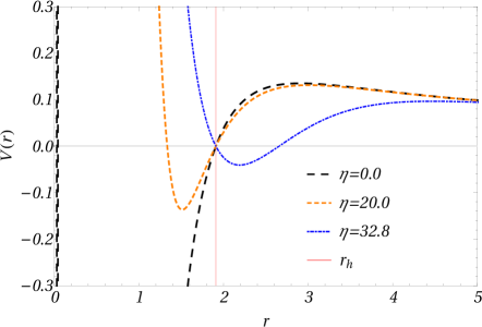
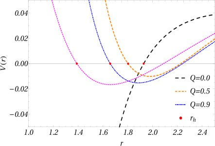
Figure 1: Effective scalar potential with parameters $M=L/10=1$ and $m=0$. Left panel: different values of $\eta$ with $l=1$ and $Q=0.2$. Right panel: different values of charge $Q$, with $l=0$ and $\eta=30$.

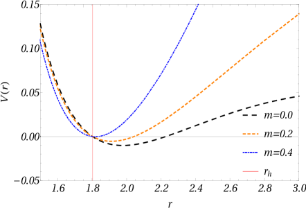
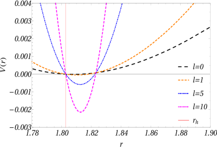
Figure 2: Effective scalar potential with parameters $M=L/10=1$. Left panel: different values of scalar field mass $m$ with $l=0$, $Q=0.5$, and $\eta=30$. Right panel: different values of multipole number $l$, $Q=0.5$, $\eta=19$, and $m=0$.

In fact, this well becomes deeper as $\eta$ approaches a critical value, $\eta_{c}$, that signals the precise moment when instabilities arise. This value can be numerically computed as we will see in the next section. As for the black hole charge, it deepens the well as long as the derivative coupling parameter $\eta$ is less than its critical value, around which the wells attain an almost uniform depth. The right panel in Fig. 1 also contains the Schwarzschild case ($Q=0$) for reference. In addition, in all figures we show the corresponding event horizon position to indicate the region of interest. In this way we can identify potentials becoming negative at some regions after this horizon, what can lead to possible instabilities.

Concerning the massive perturbation case, the effect of the multipole number $l$ and the derivative coupling parameter $\eta$ remains the same as in the massless case. In addition, the black hole charge makes the well shift outside the event horizon more quickly. Moreover, we observe that as the perturbation mass increases, the well gets shallow and the potential grows faster as can be seen in Fig. 2.

IV QNMs of a massive scalar field coupled to Einstein tensor

Based on the Klein-Gordon equation displayed in Section II, we will use the well-known characteristic integration in null-coordinates method to obtain the field propagation along with the prony method to extract the quasinormal frequencies. Both techniques were used many times in specific literature in the last years and can be found in multiple references, e. g. in Konoplya:2011qq .

The integration procedure takes place in null-coordinates $du=dt-dr_{*}$ and $dv=dt+dr_{*}$ and the boundary condition is the usual $Z|_{frontier}\rightarrow 0$. The complementar condition we take is the evolution of a gaussian wave package in the $u\times t$ diagram, with which we can analyse the field profile evolution. In cases where the field evolution goes as a damped oscillation we can extract the quasinormal modes with the prony method.

In order to check the quasi-frequencies obtained we use as a second tool a Frobenius-like method, based on the expansion of the wave function around the event horizon (developed by Horowitz and Hubeny in Horowitz:1999jd ).

IV.1 Field Propagation and QNMs

The characteristic integration in a Reissner-Nordström geometry for the Klein-Gordon field has been obtained for a multiple range of parameters. The general behavior of a quasinormal oscillation takes place for the geometry without coupling as exemplified in the cases $l=0$ and $l=1$, and for various values of $\eta$. The results we obtained with the combination of both methods are quite similar to those seen in the literature. For large black holes and cosmological constant we obtained $\omega_{l=0}=184.99-266.33I$ and $\omega_{l=3}=185.04-266.32I$ with a difference smaller than $0.03\%$ as compared with the results given in Wang:2000gsa .

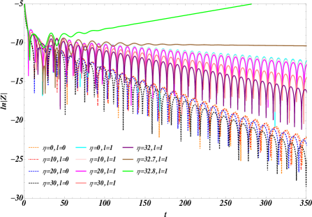
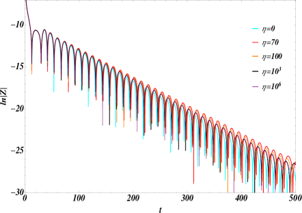
Figure 3: Scalar field behaviour for an AdS charged black hole, with varying $\eta$. The parameters of the metric are $M=L/10=5Q=1$.

In Fig. 3, left and right panels, we see typical evolutions of the scalar field obtained in the AdS charged geometry. The field evolution in the massless case is stable and performing a damped oscillation profile for every $\eta$ when the wave has no angular momentum. This is also the case for other geometry parameters: the field is stable whenever $l=0$, decaying as quasinormal signal or exponentially. Otherwise, for a scalar field with $l>0$ there is always a maximum value for $\eta$ for which the evolution remains bounded. In the above-mentioned figures, for instance, if $\eta>32.7$ (and $<100/3$) when $l>0$, the evolution will be unstable. In this case the geometry of the spacetime is expected to evolve as well and such a change has to be investigated with the full non-linear Einstein equations, what is beyond the scope of this work.

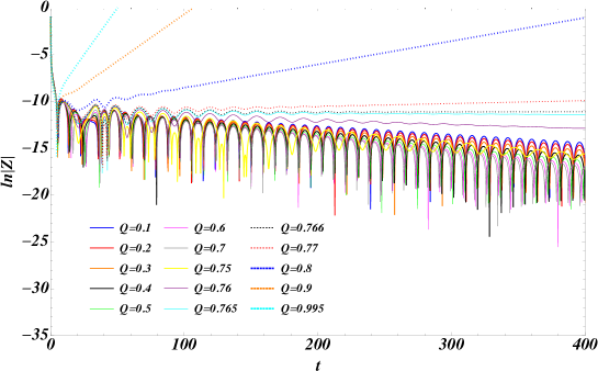
Figure 4: Scalar field behaviour for an AdS charged black hole with different charges. The parameters of the metric are $M=L/10=\eta/20=1$. There is a critical value of $Q$ from which the field destabilizes.

For high values of $\eta$ the evolution of the scalar field is almost the same as we vary $\eta$, what we can see in Fig. 3, right panel. Moreover, the quasinormal modes remain unaffected in this case, i.e., the coupling does not influence the spectra of the black hole, as we show in the next subsection.

In Fig. 4, we can see typical evolutions of the scalar field profiles in charged black holes. They are qualitatively the same evolution obtained in the Reissner-Nordström-AdS case ($\eta=0$), except near (and after) a threshold charge. In that case, $Q\sim 0.765$. Whenever $Q<0.766$ the field evolves stably, first with a ring-down signal and for charges near the critical point, as an exponential decay. On the other hand, if $Q>0.766$, the field destabilizes and the geometry must change.

The critical value of $\eta$ for which the scalar field is not stable depends on the parameters of the geometry, as expected, and notably on the angular momentum of the field.

$10M=L=10$
$l$	$Q=0.1$	$Q=0.2$	$Q=0.4$	$Q=0.6$	$Q=0.8$	$Q=0.95$	$Q=0.99517$
1	$33.15^{{}^{{}^{\pm 0.05}}}$	$32.75^{{}^{{}^{\pm 0.05}}}$	$30.65^{{}^{{}^{\pm 0.05}}}$	$26.35^{{}^{{}^{\pm 0.05}}}$	$18.25^{{}^{{}^{\pm 0.05}}}$	$7.95^{{}^{{}^{\pm 0.05}}}$	$1.75^{{}^{{}^{\pm 0.05}}}$
2	$33.05^{{}^{{}^{\pm 0.05}}}$	$32.15^{{}^{{}^{\pm 0.05}}}$	$28.65^{{}^{{}^{\pm 0.05}}}$	$22.35^{{}^{{}^{\pm 0.05}}}$	$13.45^{{}^{{}^{\pm 0.05}}}$	$5.25^{{}^{{}^{\pm 0.05}}}$	$1.25^{{}^{{}^{\pm 0.05}}}$
3	$32.95^{{}^{{}^{\pm 0.05}}}$	$31.85^{{}^{{}^{\pm 0.05}}}$	$27.45^{{}^{{}^{\pm 0.05}}}$	$20.35^{{}^{{}^{\pm 0.05}}}$	$11.55^{{}^{{}^{\pm 0.05}}}$	$4.35^{{}^{{}^{\pm 0.05}}}$	$1.15^{{}^{{}^{\pm 0.05}}}$
Lowest limit of stability for large $l$ using Eq.(22)
$\infty$	32.54	30.29	22.91	14.44	7.10	2.63	0.92

Table 1: Critical value of $\eta$ for the scalar field for different charges of the geometry (in unities of $Q_{ext}$) and angular momentum of the field. For the geometry parameters, $Q_{ext}\sim 0.99518$. The corresponding values of $\eta_{lim}$ are also shown for reference.

In Table 1 we list some of these values for the Reissner-Nordström-AdS black hole. We observe that the higher the value of the charge in the geometry is, the smaller the value of critical $\eta$ will be, the same being true for other multipole numbers. The transitional value of $\eta$ in relation to the stability of the scalar field achieves the highest gap from $l=1$ to $l=3$ around $Q=0.8Q_{ext}$ and decreases at the extremal charge. For example, if $Q=0.1Q_{ext}$, the value of transition in $\eta$ varies slowly from $l=1$ to $l=3$ (circa $0.6\%$), while for $Q=0.8Q_{ext}$, from $l=1$ to $l=3$ the variation for $\eta$ increases to $36.7\%$ and for $Q=0.99999Q_{ext}$, $34.3\%$. This means that accreting charge in a Schwarzschild black hole (with a higher rate than the accretion of mass) causes the reduction of the range of stability in $\eta$ for which the scalar field evolution decays in time.

In Fig. 5 we plotted our results for critical values of $\eta$ as a function of the black hole charge (in units of $Q_{ext}$). We also show the corresponding fitting chosen to be the simplest function of a power of the charge with three parameters,

$$\eta_{c}=33.570-32.184\,(Q/Q_{ext})^{1.779}\,.$$ (18)

This fitting produces a factor $R^{2}=0.99994$, where we define

$$R^{2}\equiv 1-\frac{\sum\limits_{i}(y_{i}-f_{i})^{2}}{\sum\limits_{i}(y_{i}-\bar{y})^{2}}\,,$$ (19)

being $y_{i}$ and $\bar{y}$ the data we numerically calculated and their corresponding mean value and $f_{i}$, the value produced by the fitting function. Clearly, the value $R^{2}=1$ means a perfect fitting. This shows the excellent correlation with the points numerically calculated.

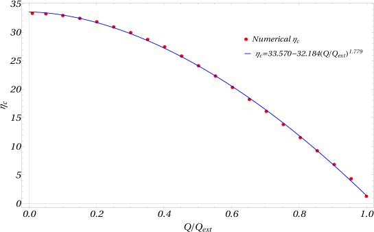
Figure 5: Critical value of $\eta$ as a function of the charge (in units of $Q_{ext}$) in Reissner-Nordström-AdS black hole. The parameters of the metric are $M=L/10=1$ and for the field $m=0$ and $l=3$.

The instability of the scalar field increases for increasing $\eta$ up to $L^{2}/3$. After this value the field transformation we used generates a discontinuity in the potential for $r>r_{h}$, and we shall not study the region of parameters for which $r_{d}>r_{h}$ until $r_{d}$ for high enough $\eta$ becomes imaginary. At this point the discontinuity disappears and the integration of the scalar field equation produces only stable evolutions, in as much as the potential is positive definite again.

In order to gain some insight about the critical value of $\eta$ let us analyse the behaviour of the effective potential near the horizon. In this region it can be rewritten as $V_{r_{h}}\sim F(r)\ \Omega(r_{h})$ where

$$\Omega(r_{h}) = \frac{m^{2}r_{h}^{2}+l(l+1)\left[1-\left(\frac{3}{L^{2}}+\frac{Q^{2}}{r_{h}^{4}}\right)\eta\right]}{r_{h}^{2}\left[1+\left(-\frac{3}{L^{2}}+\frac{Q^{2}}{r_{h}^{4}}\right)\eta\right]}+\frac{F^{\prime}(r_{h})}{r_{h}}-\frac{2Q^{2}\eta F^{\prime}(r_{h})}{r_{h}^{5}\left[1+\left(-\frac{3}{L^{2}}+\frac{Q^{2}}{r_{h}^{4}}\right)\eta\right]}$$ (20)

Since $F(r)$ is a positive function, the change of sign in the potential necessarily comes from $\Omega(r_{h})$. In this way, if the potential turns to be negative at some regions, unstable modes could in principle be turned on. Thus, we search for the zeros of $\Omega(r_{h})$ and find the value of $\eta$ when this change of sign happens,

$$\eta_{0}\sim\frac{-3L^{2}r_{h}^{8}+L^{4}r_{h}^{4}\left[Q^{2}-r_{h}^{2}\left(1+l(l+1)+m^{2}r_{h}^{2}\right)\right]}{\left(L^{2}Q^{2}+3r_{h}^{4}\right)\left\{-3r_{h}^{4}+L^{2}\left[Q^{2}-r_{h}^{2}(1+l(l+1))\right]\right\}}.$$ (21)

The first thing we notice is that when $m=0$, Eq.(21) becomes independent of $l$ and is reduced to the limit value,

$$\eta_{lim}\sim\frac{L^{2}r_{h}^{4}}{L^{2}Q^{2}+3r_{h}^{4}}$$ (22)

This same result also corresponds to the limit when $l\rightarrow\infty$, i.e., for large multipole numbers. This independence can be seen in the right panel of Fig. 2. For large $l$ the zeros of the potential remain at the same position and $l$ only affects the well depth. Moreover, our calculations show that as $l$ increases, $\eta_{c}$ approaches $\eta_{lim}$ as we can see in Table 1. For instance, the numerical results for large $l$ resemble the approximation above listed in table I. If we take $M=0.1L=5Q=l/50=1$, then $\eta_{c}\sim 30.45$, only $0.5\%$ away from the listed value for $l\rightarrow\infty$. Thus, $\eta_{lim}$ can be considered the lowest limit of stability for large $l$.

Inspired by Eq.(21) we also found an alternative fitting for the numerical data in Fig. 5 given by

$$\eta_{c}=\frac{8.103-7.617\,(Q/Q_{ext})^{2}}{\left[0.518+0.004\,(Q/Q_{ext})\right]\left[0.469+0.091\,(Q/Q_{ext})^{2}\right]}\,,$$ (23)

which has a similar $R^{2}$ factor as Eq.(18) showing excellent agreement with the numerical data.

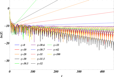
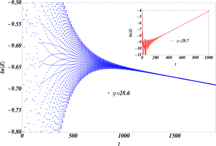
Figure 6: Scalar field evolution for multiple values of $\eta$ on the charged AdS black hole. The parameters of the metric are $M=L/10=2.5Q=1$ and for the field $l=1$ (left) and $l=2$ (right). The threshold of stability for $\eta$ is different for each $l$. In the left panel we see a critical coupling constant $\eta_{c}\sim 30.65$, and in the right panel $\eta_{c}\sim 28.65$ (the blue points presenting a stable evolution and the red one unstable).

In Fig. 6 we can see examples of this limiar of stability, for $l=1$ and $l=2$. In the first case $\eta_{c}\sim 30.6$ and for $\eta>62$ only stable evolutions are seen for every $l$. The same behavior is seen in the right panel for $l=2$ in which $\eta_{c}\sim 28.6$, and again for $\eta>62$ only stable profiles are generated. In cases of very high $\eta$ no difference is noticed in the field evolution as shown in Fig. 3: for $\eta=10^{3}$ to $10^{40}$ all signals collapse to a single one.

The situation is qualitatively similar when we study the coupling for large black holes and large $\Lambda$. In such a case it is not possible to verify qualitative changes in the quasinormal spectra from that of an AdS black hole without coupling and the quasinormal modes are marginally affected except when $\eta\sim\frac{L^{2}}{3}$ (we compute some examples in the next subsection). This comes with no surprise if we look at Table 1 and Fig. 6: whenever $\eta>\eta_{c}$, the field destabilizes more and more as $\eta$ approaches $\frac{L^{2}}{3}$. Thus, for black holes with high $r_{h}$, a discerning influence is generated in the field propagation only for $\eta\sim\Lambda^{-1}$. As we may further see, the quasinormal modes do not change in such cases.

IV.2 The quasinormal frequencies

The quasinormal frequencies obtained for the Reissner-Nordström-AdS black hole are mostly affected by the scalar field coupling in the limit of small $r_{h}$ and $L$. In the cases of high $r_{h}$ or $\eta>>\Lambda^{-1}$, the effect of the coupling is very mild.

Table 2: The quasinormal modes of the RNAdS black hole with $l=0$.

$M=L/10=5Q=1$			$r_{h}=5Q=50L=50$
$\eta$	$\operatorname{Re}(\omega)$	$-\operatorname{Im}(\omega)$	$\eta$	$\operatorname{Re}(\omega)$	$-\operatorname{Im}(\omega)$
70	0.2443	0.03371	0	92.548	133.17
100	0.2452	0.03437	0.3	92.551	133.18
1000	0.2462	0.03507	0.33	92.579	133.30
$10^{6}$	0.2463	0.03511	0.333	92.891	134.50
$10^{12}$	0.2463	0.03511	0.3333	100.20	146.53
$10^{40}$	0.2463	0.03511	1	92.548	133.17

In Table 2, the frequencies vary less than $0.2\%$ for every $\eta>30\Lambda^{-1}$ for small black holes. On the other hand, in the limit of high $r_{h}$, the scalar field spectrum remains unaffected for the coupling except very near $\Lambda^{-1}$: the quasinormal mode is exactly the same (to the fifth figure) for $\eta=0$ and every $\eta>1$. A similar behavior is obtained varying the parameters, maintaining $r_{h}$ high: if we take, e. g., $r_{h}=Q=100L=100$ and $l=0$, the fundamental mode is $\omega=184.95-266.38I$ for $\eta=0$ and $\omega=184.95-266.36I$ for every $\eta\geq 1$, which also occurs for other values of $l$.

Table 3: The quasinormal modes of the RNAdS black hole with $M=L/10=1$ and $l=0$.

$\eta$	$Q=0.1$		$Q=0.2$		$Q=0.4$		$Q=0.6$		$Q=0.8$		$Q=0.95$
	$\operatorname{Re}(\omega)$	$-\operatorname{Im}(\omega)$	$\operatorname{Re}(\omega)$	$-\operatorname{Im}(\omega)$	$\operatorname{Re}(\omega)$	$-\operatorname{Im}(\omega)$	$\operatorname{Re}(\omega)$	$-\operatorname{Im}(\omega)$	$\operatorname{Re}(\omega)$	$-\operatorname{Im}(\omega)$	$\operatorname{Re}(\omega)$	$-\operatorname{Im}(\omega)$
0	0.2453	0.03664	0.2483	0.03641	0.2477	0.03542	0.2464	0.03372	0.2440	0.03125	0.2407	0.02962
5	0.2486	0.03669	0.2487	0.03661	0.2492	0.03625	0.2505	0.03551	0.2533	0.03363	0.2559	0.02959
10	0.2487	0.03676	0.2492	0.03689	0.2514	0.03721	0.2556	0.03688	0.2614	0.03395	0.2645	0.02905
15	0.2489	0.03687	0.2500	0.03730	0.2545	0.03830	0.2616	0.03760	0.2687	0.03347	0.2716	0.02880
20	0.2493	0.03706	0.2513	0.03794	0.2592	0.03938	0.2688	0.03754	0.2761	0.03285	0.2786	0.02896
25	0.2500	0.03746	0.2541	0.03905	0.2669	0.03997	0.2779	0.03673	0.2847	0.03246	0.2872	0.02966
30	0.2528	0.03879	0.2632	0.04101	0.2818	0.03886	0.2925	0.03590	0.2995	0.03423	***	***

In Table 3 we can see the effect of $\eta$ coupling in the quasinormal spectra for a small black hole. The influence is again more pronounced in the regions $\eta\sim\Lambda^{-1}$ specially for high values of charge. In general the field profile rapidly undergoes the exponential decay for $\eta$ near $\Lambda^{-1}$. For example, no oscillation forms for $Q=0.95$ and $\eta=30$. The oscillation of the values of the quasinormal modes (increasing and decreasing with increasing charge) is an expected feature already demonstrated in other references Wang:2004bv .

In addition, quasinormal frequencies were calculated using another numerical approach, developed by Horowitz and Hubeny Horowitz:1999jd , as a double check. As is usually the case, this method produces the best results for large $r_{h}$, while for small $r_{h}$ the convergence of the method is problematic. The values we found are in good agreement with the previous method and the difference between these values is around $0.05\%$ for the real part and $0.03\%$ for the imaginary part of the frequencies when $\eta$ is far from the critical value. Near $\eta_{c}$ the convergence of Horowitz-Hubeny method shows to be very poor.

V Final remarks

In the present work we have investigated the influence of a non-minimal derivative coupling $\eta$ of a massive scalar field coupled to Einstein tensor on the propagation of this field in the vicinity of a Reissner-Nordström-AdS black hole. We carried out a detailed investigation of the regions of instability of the background black hole which arise depending upon the value of $\eta$ and the parameters of the theory, namely the mass $M$ and the electric charge $Q$ of the black hole, the AdS radius $L$ and also the scalar field multipole number $l$ and its mass $m$.

In the case of massless scalar perturbations the effective potential develops a negative well, which can be shifted from inside the event horizon to the exterior region as the derivative coupling parameter $\eta$ grows and can be made deep enough depending on the region of parameters. The development of a negative well indicates possible instabilities of the background Reissner-Nordström-AdS black hole and it is confirmed by the analysis of field propagation through the computation of quasinormal modes and frequencies. In the case of massive scalar perturbations as the perturbation mass increases, the well gets shallow and the potential grows faster.

In the case of zero angular momentum the massless scalar field evolves stably whatever the value of $\eta$ is. However, for non-zero angular momentum we found a critical value of the derivative coupling $\eta_{c}$ above which the scalar field propagates unstable modes. Looking at the QNMs we observed that as we increase $\eta$ above its critical value $\eta_{c}$, the oscillations are getting slower and the QNMs decay faster. This behaviour is expected because as we already discussed, the coupling of the scalar field to Einstein tensor strongly influences its kinetic energy.

Regarding the effect of the black hole charge $Q$, we found that as the charge $Q$ is approaching its extremal value $Q_{ext}$, the critical value $\eta_{c}$ is decreasing. A similar behaviour was observed in a charged rotating black hole. It was found that instabilities can appear when the angular momentum of the black hole is small, as long as the charge is sufficiently large Andrade:2018rcx ; Tanabe:2016opw .

Finally, as we already discussed, for values of $\eta$ beyond $\eta_{c}$ the field develop instabilities. However, we observed that stability is recovered after a certain value of $\eta>\eta_{c}$, featuring two transitions of the scalar field propagation from stability to instability and going back to stable quasinormal oscillation. This is an intriguing effect indicating a kind of phase transition from an unstable to a stable configuration, observed also in de Sitter geometries EtadS .

This behaviour may signals that the Reissner-Nordström-AdS black hole is scalarized, i.e., it acquires hair and it gets stabilized. Actually a similar behaviour was found in Doneva:2018rou in which the extended scalar-tensor-Gauss-Bonnet gravity was studied and it was found that a scalar field, sourced by the curvature of the spacetime via the Gauss-Bonnet invariant, scalarized spontaneously the Reissner-Nordström-AdS black hole. We intend to further study this effect in a fully backreacting problem with the scalar field interacting with the background metric in a future project.

VI Acknowledgments

This work was supported by CNPq (Conselho Nacional de Desenvolvimento Científico e Tecnológico), FAPESP (Fundação de Amparo à Pesquisa do Estado de São Paulo), and FAPEMIG (Fundação de Amparo à Pesquisa do Estado de Minas Gerais), Brazil. E.P. acknowledges the hospitality of the Physics Institute of the University of São Paulo where this work started and CNPq for financial support.

References

- (1) G. W. Horndeski, Int. J. Theor. Phys. 10 (1974) 363-384.
- (2) A. Nicolis, R. Rattazzi, E. Trincherini, “The Galileon as a local modification of gravity,” Phys. Rev. D79 (2009) 064036. [arXiv:0811.2197 [hep-th]].
- (3) C. Deffayet, G. Esposito-Farese, A. Vikman, “Covariant Galileon,” Phys. Rev. D79 (2009) 084003. [arXiv:0901.1314 [hep-th]].
- (4) C. Deffayet, S. Deser and G. Esposito-Farese, “Generalized Galileons: All scalar models whose curved background extensions Phys. Rev. D 80, 064015 (2009) [arXiv:0906.1967].
- (5) L. Amendola, “Cosmology with nonminimal derivative couplings,” Phys. Lett. B 301, 175 (1993) [arXiv:gr-qc/9302010].
- (6) S. V. Sushkov, “Exact cosmological solutions with nonminimal derivative coupling,” Phys. Rev. D 80, 103505 (2009) [arXiv:0910.0980 [gr-qc]].
- (7) E. N. Saridakis and S. V. Sushkov, “Quintessence and phantom cosmology with non-minimal derivative coupling,” Phys. Rev. D 81, 083510 (2010) [arXiv:1002.3478 [gr-qc]].
- (8) L. N. Granda, D. F. Jimenez and C. Sanchez, “Quintessential and phantom power-law solutions in scalar tensor model of dark energy,” Int. J. Mod. Phys. D 22, 1350055 (2013), [arXiv:1211.3457 [astro-ph.CO]].
- (9) C. Germani, A. Kehagias, “New Model of Inflation with Non-minimal Derivative Coupling of Standard Model Higgs Boson to Gravity,” Phys. Rev. Lett. 105, 011302 (2010). [arXiv:1003.2635 [hep-ph]].
- (10) S. Tsujikawa, “Observational tests of inflation with a field derivative coupling to gravity,” Phys. Rev. D 85, 083518 (2012) [arXiv:1201.5926 [astro-ph.CO]].
- (11) G. Koutsoumbas, K. Ntrekis and E. Papantonopoulos, “Gravitational Particle Production in Gravity Theories with Non-minimal Derivative Couplings,” JCAP 1308, 027 (2013) [arXiv:1305.5741 [gr-qc]].
- (12) H. M. Sadjadi and P. Goodarzi, “Reheating in nonminimal derivative coupling model,” JCAP 1302, 038 (2013) [arXiv:1203.1580 [gr-qc]].
- (13) L. Hui and A. Nicolis, “A no-hair theorem for the galileon,” Phys. Rev. Lett. 110, 241104 (2013) [arXiv:1202.1296 [hep-th]].
- (14) M. Rinaldi, “Black holes with non-minimal derivative coupling,” Phys. Rev. D 86, 084048 (2012) [arXiv:1208.0103 [gr-qc]].
- (15) T. Kolyvaris, G. Koutsoumbas, E. Papantonopoulos and G. Siopsis, “Scalar Hair from a Derivative Coupling of a Scalar Field to the Einstein Tensor,” Class. Quant. Grav. 29, 205011 (2012) [arXiv:1111.0263 [gr-qc]].
- (16) T. Kolyvaris, G. Koutsoumbas, E. Papantonopoulos and G. Siopsis, “Phase Transition to a Hairy Black Hole in Asymptotically Flat Spacetime,” JHEP 1311, 133 (2013) [arXiv:1308.5280 [hep-th]].
- (17) E. Babichev and C. Charmousis, “Dressing a black hole with a time-dependent Galileon,” JHEP 1408, 106 (2014) [arXiv:1312.3204 [gr-qc]].
- (18) C. Charmousis, T. Kolyvaris, E. Papantonopoulos and M. Tsoukalas, “Black Holes in Bi-scalar Extensions of Horndeski Theories,” JHEP 1407, 085 (2014) [arXiv:1404.1024 [gr-qc]].
- (19) A. Anabalon, A. Cisterna and J. Oliva, “Asymptotically locally AdS and flat black holes in Horndeski theory,” Phys. Rev. D 89, 084050 (2014), [arXiv:1312.3597 [gr-qc]]; M. Minamitsuji, “Solutions in the scalar-tensor theory with nonminimal derivative coupling,” Phys. Rev. D 89, 064017 (2014), [arXiv:1312.3759 [gr-qc]]; A. Cisterna and C. Erices, “Asymptotically locally AdS and flat black holes in the presence of an electric field in the Horndeski scenario,” Phys. Rev. D 89, 084038 (2014) [arXiv:1401.4479 [gr-qc]].
- (20) E. Babichev, C. Charmousis and M. Hassaine, “Charged Galileon black holes,” JCAP 1505, 031 (2015) [arXiv:1503.02545 [gr-qc]].
- (21) T. P. Sotiriou and S. Y. Zhou, “Black hole hair in generalized scalar-tensor gravity: An explicit example,” Phys. Rev. D 90, 124063 (2014) [arXiv:1408.1698 [gr-qc]].
- (22) R. Benkel, T. P. Sotiriou and H. Witek, “Black hole hair formation in shift-symmetric generalised scalar-tensor gravity,” Class. Quant. Grav. 34, no. 6, 064001 (2017) [arXiv:1610.09168 [gr-qc]].
- (23) S. Chen and J. Jing, “Dynamical evolution of a scalar field coupling to Einstein’s tensor in the Reissner-Nordström black hole spacetime,” Phys. Rev. D 82, 084006 (2010) [arXiv:1007.2019 [gr-qc]].
- (24) S. S. Gubser, “Breaking an Abelian gauge symmetry near a black hole horizon,” Phys. Rev. D 78, 065034 (2008) [arXiv:0801.2977 [hep-th]].
- (25) M. Minamitsuji, “Black hole quasinormal modes in a scalar-tensor theory with field derivative coupling to the Einstein tensor,” Gen. Rel. Grav. 46, 1785 (2014) [arXiv:1407.4901 [gr-qc]].
- (26) S. Yu and C. Gao, “Quansinormal modes of static and spherically symmetric black holes with the derivative coupling,” Gen. Rel. Grav. 51, no. 1, 16 (2019) [arXiv:1807.05024 [gr-qc]].
- (27) R. A. Konoplya, Z. Stuchlik and A. Zhidenko, “Massive nonminimally coupled scalar field in Reissner-Nordstrom spacetime: Long-lived quasinormal modes and instability,” Phys. Rev. D 98, no. 10, 104033 (2018) [arXiv:1808.03346 [gr-qc]].
- (28) E. Abdalla, B. Cuadros-Melgar, J. de Oliveira, A. B. Pavan and C. E. Pellicer, “Vectorial and spinorial perturbations in Galileon black holes: Quasinormal modes, quasiresonant modes, and stability,” Phys. Rev. D 99, no. 4, 044023 (2019) [arXiv:1810.01198 [gr-qc]].
- (29) T. Kolyvaris and E. Papantonopoulos, “Superradiant Amplification of a Scalar Wave Coupled Kinematically to Curvature Scattered off a Reissner-Nordström Black Hole,” arXiv:1702.04618 [gr-qc].
- (30) T. Kolyvaris, M. Koukouvaou, A. Machattou and E. Papantonopoulos, “Superradiant instabilities in scalar-tensor Horndeski theory,” Phys. Rev. D 98, no. 2, 024045 (2018) [arXiv:1806.11110 [gr-qc]].
- (31) G. Koutsoumbas, I. Mitsoulas and E. Papantonopoulos, “Quantum Effects in Galileon Black Holes,” Class. Quant. Grav. 35, no. 23, 235016 (2018) [arXiv:1803.05489 [gr-qc]].
- (32) R. A. Konoplya and A. Zhidenko, “Quasinormal modes of black holes: From astrophysics to string theory,” Rev. Mod. Phys. 83, 793 (2011) [arXiv:1102.4014 [gr-qc]].
- (33) G. T. Horowitz and V. E. Hubeny, “Quasinormal modes of AdS black holes and the approach to thermal equilibrium,” Phys. Rev. D 62, 024027 (2000) [hep-th/9909056].
- (34) B. Wang, C. Y. Lin and E. Abdalla, “Quasinormal modes of Reissner-Nordström anti-de Sitter black holes,” Phys. Lett. B 481, 79 (2000) [hep-th/0003295].
- (35) B. Wang, C. Y. Lin and C. Molina, “Quasinormal behavior of massless scalar field perturbation in Reissner-Nordstrom anti-de Sitter spacetimes,” Phys. Rev. D 70, 064025 (2004) [hep-th/0407024]; E. Berti and K. D. Kokkotas, “Asymptotic quasinormal modes of Reissner-Nordstrom and Kerr black holes,” Phys. Rev. D 68, 044027 (2003) [hep-th/0303029].
- (36) T. Andrade, R. Emparan and D. Licht, “Charged rotating black holes in higher dimensions,” JHEP 1902, 076 (2019) [arXiv:1810.06993 [hep-th]].
- (37) K. Tanabe, “Charged rotating black holes at large D,” arXiv:1605.08854 [hep-th].
- (38) R. D. B. Fontana, Jeferson de Oliveira and A. B. Pavan, “Dynamical evolution of non-minimally coupled scalar field in spherically symmetric de Sitter spacetimes”, [arXiv:1808.01044 [gr-qc]].
- (39) D. D. Doneva, S. Kiorpelidi, P. G. Nedkova, E. Papantonopoulos and S. S. Yazadjiev, “Charged Gauss-Bonnet black holes with curvature induced scalarization in the extended scalar-tensor theories,” Phys. Rev. D 98, no. 10, 104056 (2018) [arXiv:1809.00844 [gr-qc]].