Quantized alternate current on curved graphene

Abstract

Based on the numerical solution of the quantum lattice Boltzmann method in curved space, we predict the onset of a quantized alternating current on curved graphene sheets. Such numerical prediction is verified analytically via a set of semi-classical equations relating the Berry curvature to real space curvature. The proposed quantised oscillating current on curved graphene could form the basis for the implementation of quantum information processing algorithms.

I Introduction

In recent years, the most puzzling features of quantum mechanics, such as entanglement and non-local "spooky action at distance", long regarded as a sort of extravagant speculations, have received spectacular experimental confirmation EPR; bell; Aspect; Haroche. Besides their deep fundamental implications, such phenomena may also open up transformative scenarios for material science and related applications in quantum computing and telecommunications bennett; Zeilinger. Along with such burst of experimental activity, a corresponding upsurge of theoretical and computational methods has also emerged in the last two decades, including, among others, new quantum-many body techniques, quantum simulators cirac; blochImanuel; quantumsim; quantization and quantum walks quantumenta.

Quantum walks were first introduced by Aharonov and collaborators in 1993 Aharanov, just a few months before the appearance of the first quantum lattice Boltzmann scheme succi_qlbm, which was only recently recognized to be a quantum walk too succiQW. Quantum walks quantumwalk2; quantumwalk3 are currently utilized to investigate exotic states of quantum matter majorana and to design new materials and technologies for quantum engineering applications quantumwalk.

Quantum walks can also help exploring the emergence of classical behaviour in the limit of a vanishing De Broglie length quantummechanics. Likewise, quantum cellular automata cellularautomata1; cellularautomata2; cellularautomata3, can be used for simulating complex systems in analogy with their classical counterparts.

Finally, quantum walks have also shown connections with topological aspects of quantum mechanics, most notably the Berry phase Berry. Indeed, Berry connection and Berry curvature can be understood as a local gauge potential and gauge field, respectively and they define a Berry phase as introduced in 1984 Berry. The Berry phase has important implications as an analytic tool in topological phases of matter topologicalstatesofmatter and, under suitable conditions, it can also be related to real space curvature ryder, thus providing a potential bridge between the classical and quantum descriptions of a given system.

As of quantum materials, graphene presents one of the most promising cases for realizing a new generation of quantum devices graphenerev1; graphenerev2; graphenerev3. Indeed, since its discovery Geim-graphene, this flatland wonder-material has not ceased to surprise scientists with its amazing mechanical and electronic behaviour. For example, stacking graphene sheets at specific angles has shown spectacular indications of superconductivity and other exotic properties magic_angle.

Tunable transport properties are a basic requirement in electronic devices and specifically in graphene tunable. Furthermore, it has been shown that graphene sheets can be curved in such a way as to trap particles cdp, thus opening further prospects for technological applications based on localized quantum states.

In this work, we propose the generation of a quantized oscillating current on curved graphene, which could be used in conjunction with trapped fermions for the realization of quantum cellular automata.

Electron transport is simulated by numerically solving the Dirac equation in curved space JD_thesis; cdp using an extension to curved space of the quantum lattice Boltzmann method succi_qlbm. In addition, a simpler representation of the system is solved analytically through a set of semi-classical equations of motion, relating Berry to real space curvature.

The paper is organized as follows. First, we introduce the Dirac equation and its extension to curved space and specifically deformed graphene. In the subsequent section, we present the results of numerical simulations and finally we conclude with a summary and outlook section. A detailed description of the numerical model is provided in the Appendix (Appendix LABEL:sec:QLBM).

II The Dirac equation in curved space and graphene

The Dirac equation in curved space can be written in compact notation as follows:

$$(i\gamma^{\mu}D_{\mu}-m)\Psi=0,$$ (1)

in natural units $\hbar=c=1$, where $m$ is the particle rest mass, the index $\mu={0,1,2}$ runs over 2D space-time. In the above, $\Psi=(\Psi^{+},\Psi^{-})=(\psi_{1}^{+},\psi_{2}^{-},\psi_{1}^{-},\psi_{2}^{+})\in\mathbbm{C}^{4}$ denotes the Dirac four-spinor, and $\gamma^{\mu}=\gamma^{\alpha}e_{\alpha}^{\ \mu}$ are the generalized $\gamma$-matrices, where $\gamma^{\alpha}\in\mathbbm{C}^{4\times 4}$ are the standard $\gamma$-matrices (in Dirac representation). The symbol $e_{\alpha}^{\ \mu}$ is the tetrad (first index: flat Minkowski, second index: curved space-time).

Here, the tetrad is defined by $e_{\alpha}^{\mu}g_{\mu\nu}e_{\beta}^{\nu}=\eta_{\alpha\beta}$ kaku1993quantum, where $g_{\mu\nu}$ denotes the metric tensor and $\eta_{\alpha\beta}$ is the Minkowski metric. The tetrad basis is chosen such that the standard Dirac matrices can be utilised with no need to transform to a new coordinate basis. The symbol $D_{\mu}$ denotes the covariant spinor derivative, defined as $D_{\mu}\Psi=\partial_{\mu}\Psi+\Gamma_{\mu}\Psi$, where $\Gamma_{\mu}$ denotes the spin connection matrices given by $\Gamma_{\mu}=-\frac{i}{4}\omega_{\mu}^{\alpha\b{}}\sigma_{\alpha\b{}},$ where $\sigma_{\alpha\b{}}=\frac{i}{2}[\gamma_{\alpha},\gamma_{\b{]}}$ and $\omega_{\mu}^{\alpha\b{}}=\quad e_{\nu}^{\alpha}{\nabla}_{\mu}e^{\nu\b{}}$ The Dirac equation in curved space describes quantum relativistic Dirac particles (e.g. electrons ) moving on arbitrary manifold trajectories.

The covariant derivative ensures the independence of the Dirac equation of the coordinate basis. The covariance is satisfied by the connection coefficients which can be interpreted physically as a vector potential. The Poincare symmetries are obeyed by the Dirac equation ensuring the special relativistic nature of the wavefunctions. The mass term represents the Minkowski metric invariant rest mass. Interactions add to an effective mass by the very definition of covariant derivative, which places the vector potential on the same mathematical basis as a physical mass. Graphene is modeled by a mass-less Dirac Hamiltonian.

II.1 Theory of strained graphene

Using the tight binding Hamiltonian to describe the bi-partite lattice of graphene, it is established that in the low-energy limit, the dispersion relation is linear, as described by the Dirac cones at the corners of the first Brillouin zone, which can be described by the following Dirac Hamiltonian:

$$H_{D}=-i\int\Psi^{\dagger}\gamma^{0}\gamma^{i}\partial_{i}\Psi d^{2}x,$$ (2)

in natural units, where $\Psi$ is in the chiral representation.

In the context of graphene, the general Dirac spinor is defined as $\Psi=(\Psi_{a}^{K},\Psi_{a}^{K^{\prime}})=(\psi_{A}^{K},\psi_{B}^{K^{\prime}},\psi_{A}^{K^{\prime}},\psi_{B}^{K})$, for sub-lattices $A,B$ and valleys $K,K^{\prime}$.

The equation of motion stemming from this Hamiltonian is precisely the Dirac equation.

In this work, we consider a static space-time metric, with trivial time components

$$g_{\mu\nu}=\begin{pmatrix}1&0\\ 0&-g_{ij}\end{pmatrix},$$

where the latin indices run over the spatial dimensions.

This simplifies the Dirac equation Eq. (1) to

$$\partial_{t}\Psi+\sigma^{a}e_{a}^{\leavevmode\nobreak\ i}(\partial_{i}+\Gamma_{i})\Psi=0-i\gamma^{0}m\Psi,$$ (3)

with $\sigma^{a}=\gamma^{0}\gamma^{a}$. After addition of external vector and scalar potentials $A_{i}(x)$ and $V(x)$ respectively, as explained in Ref. jd_paper, the Dirac equation takes the following form:

$$\partial_{t}\Psi+\sigma^{a}e_{a}^{\leavevmode\nobreak\ i}(\partial_{i}+\Gamma_{i}-iA_{i})\Psi=-i\gamma^{0}(m-V)\Psi.$$ (4)

Defining the Dirac current as $J^{\mu}=\overline{\Psi}\gamma^{\mu}\Psi$, the charge density conservation law can be written as $\partial_{t}\rho+\nabla_{i}J^{i}=0$, where $\r{=}\Psi^{\dagger}\Psi\in\mathbbm{R}$ and the $J^{i}=\overline{\Psi}\gamma^{i}\Psi\in\mathbbm{R}$.

The standard Dirac Hamiltonian for Eq. (4) equation is given by:

$$H_{D}=-i\int\Psi^{\dagger}\sigma^{a}e_{a}^{\leavevmode\nobreak\ i}(\partial_{i}+\Gamma_{i}-iA_{i})\Psi\sqrt{g}d^{2}x,$$ (5)

For the case of graphene, the effective Hamiltonian reads as follows OLIVALEYVA:

$$H^{*}_{D}=-i\int\Psi^{\dagger}\sigma^{a}(v_{a}^{*i}\partial_{i}+\Gamma_{a}^{*}-iA^{*}_{a})\Psi d^{2}x,$$ (6)

where $v_{a}^{*i}=\d{_}{ai}+u_{ai}-\beta\varepsilon_{ai}$ is the space-dependent Fermi velocity, $\Gamma^{*}_{a}=\frac{1}{2}\partial_{j}v_{a}^{*j}$ is a complex gauge vector field which guarantees the hermicity of the Hamiltonian and $A^{*}_{a}$ is a strain-induced pseudo-vector potential, given by $A^{*}_{a}=(A_{x}^{*},A_{y}^{*})=\frac{\beta}{2a}(\varepsilon_{xx}-\varepsilon_{yy},-2\varepsilon_{xy}$). Furthermore, $\beta$ is the material-dependent electron Grueneisen parameter, $a$ the lattice spacing and $\varepsilon_{i\jmath}=u_{i\jmath}+\frac{1}{2}\partial_{i}h\partial_{j}h$ is the general strain tensor, with in-plane, $u_{i\jmath}$ and out of plane, $h$ deformations.

Comparing this to the standard Dirac Hamiltonian in curved space Eq. (5), we can match both Hamiltonians $H_{D}$ and $H^{*}_{D}$ by fulfilling the following relations:

$$v_{a}^{*i}=\sqrt{g}e_{a}^{\leavevmode\nobreak\ i},\ \ \Gamma_{a}^{*}=\sqrt{g}e_{a}^{\leavevmode\nobreak\ i}\Gamma_{i},\ \ A^{*}_{a}=\sqrt{g}e_{a}^{\leavevmode\nobreak\ i}A_{i}.$$ (7)

All three relations above can be simultaneously fulfilled by an effective metric tensor derived from the explicit expression of the tetrad jd_paper.

The numerical solutions are obtained with the Quantum Lattice Boltzmann Method, as described in Appendix LABEL:sec:QLBM and Ref. jd_paper.

III Quantized alternating current graphene strip

To investigate the potential of curvature on curved graphene sheets, we propose a periodic system with alternating current (AC) behaviour, which is quantized according to its shape. The system geometry is initialized by the discrete mapping (or chart),

$$h^{\alpha}(x,y)= \begin{pmatrix}x\\ y\\ y\sin(\eta x/2)\end{pmatrix}$$ (8)

with $x\in\{0,2\pi\}$, $y\in\{-L_{y}/2,L_{y}/2\}$, $L_{y}$ being the domain size in the $y$ dimension, see Fig. 1. The boundaries are periodic along the $x$-direction and closed at $-L_{y}/2,L_{y}/2$.

The initial condition is given by a Gaussian wave-packet of the form:

$$\Psi(\mathbf{r},\mathbf{k})=\frac{1}{\sqrt{2\pi\mathcal{\sigma}^{2}}} \begin{pmatrix}1\\ \lambda e^{i\theta}\end{pmatrix}e^{-\frac{|\mathbf{r}|^{2}}{4\mathcal{\sigma}^{2}}+i\mathbf{k}\cdot\mathbf{r}},$$ (9)

where $\lambda=\pm 1$ is the band index, $\theta=\arctan(k_{y}/k_{x})$, $\mathcal{\sigma}$ is a measure of the width, $\mathbf{r}=(x,y)$, $x,\leavevmode\nobreak\ y$ are the two space coordinates and $\mathbf{k}=(k_{x},k_{y})$, $k_{x},\leavevmode\nobreak\ k_{y}$ represent the $x$ and $y$ momenta, respectively.

The initial values are taken as $k_{x}=1$, $k_{y}=0$ and $\lambda=1$. In the simulations, we consider a rectangular sheet with periodic boundary conditions on a grid of size $L_{x}\times L_{y}=256\times 128$ or $20nm\times 5nm$, while the external potential $A_{a}$ is set to zero. Therefore, the subsequent motion is purely curvature-driven.

The discretization of the real space shape of the graphene strip, is plotted in Fig. 1(a). The norm of the wave-function, $\left\lVert\Psi\right\rVert^{2}$, i.e. the probability density, $\rho$ is plotted in Fig. 1(b) for the initial and a few subsequent time-steps.

As one can appreciate, the wave-packet spreads as expected, with no clear indication of motion along the $y$ direction.

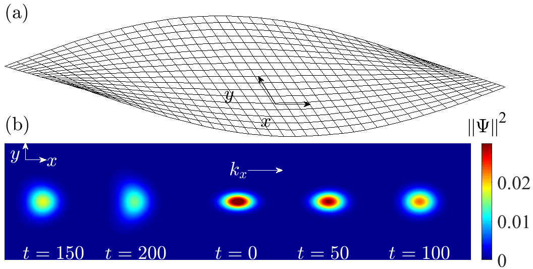
Figure 1: (a) Real space geometry of the graphene strip, $x,y$ denote the coordinate directions. (b) Density plots of the wave-packet for different time-steps, the $k_{x}$ arrow denotes the propagation direction. The bulk of the wave-packet propagates forward and is spreading as expected.

The position of the center of charge density along the $y$ direction:

$$\bar{y}=\bigg{(}\int^{area}y(\rho(t)-\rho(0))dA\bigg{)}/\int^{area}\rho(t)dA,$$ (10)

is plotted as a function of time in Fig. 2, where $dA=dxdy$.

A small but significant oscillation along the $y$ direction is observed.

These oscillations can be understood as the geometrical equivalent of the Bloch oscillations and they are a consequence of the sinusoidal, periodic domain, with the frequency quantized in units of the parameter $\eta$. For a slowly perturbed Hamiltonian and expanding around the wave-packet center $c$ (initialized to $(0,0)$ here), $H=H_{c}+\Delta H$, assuming a periodic system described by a Bloch wavefunction, the semi-classical equations of motion are given by berry_paper:

$$\dot{\mathbf{r}}_{c} =\frac{\partial\varepsilon}{\partial\mathbf{k}}-(\Omega_{\mathbf{k}\mathbf{r}}\cdot\dot{\mathbf{r}}_{c}+\Omega_{\mathbf{k}\mathbf{k}}\cdot\dot{\mathbf{k}}_{c})-\Omega_{\mathbf{k}t}$$ (11)

$$\dot{\mathbf{k}}_{c} =\frac{\partial\varepsilon}{\partial\mathbf{r}}-(\Omega_{\mathbf{r}\mathbf{k}}\cdot\dot{\mathbf{k}}_{c}+\Omega_{\mathbf{r}\mathbf{r}}\cdot\dot{\mathbf{r}}_{c})-\Omega_{\mathbf{r}t}$$ (12)

where $\mathbf{r}_{c},\mathbf{k}_{c}$ are the center of mass position and momentum of the wavepacket, $\mathbf{r},\mathbf{k}$ are the position and momentum vectors, $t$ is time, $\varepsilon$ is the band energy and $\Omega_{\mathbf{k}\mathbf{r}}=(\Omega_{\mathbf{k}\mathbf{r}})_{\alpha\b{}}=\partial\mathbf{k}_{\alpha}\mathcal{A}_{\mathbf{r}_{\b{}}}-\partial\mathbf{r}_{\b{\mathcal{missing}}}{A}_{\mathbf{k}_{\alpha}}$ is the Berry curvature and $\mathcal{A}_{\mathbf{r}}$ the Berry connection.

As shown in the Appendix LABEL:app:berry_phase, the Berry phase, and thus Berry curvature, can be related directly to the spin connection $\Gamma_{\mu}$ through $\mathcal{A}^{i}_{n}(\mathbf{R})=i\langle\Psi(\mathbf{R})|\partial_{\mathbf{R}}|\Psi(\mathbf{R})\rangle\implies\mathcal{A}_{R_{i}}=\operatorname{Tr}\langle\Psi|\Gamma_{i}|\Psi\rangle$ for some parameter space $\mathbf{R}$ and eigen-function index $n$.

The non zero terms of Eqs. (11,12) for the specific geometry are $\dot{\mathbf{r}}_{c}=\partial\varepsilon/\partial\mathbf{k}\approx v_{f},\leavevmode\nobreak\ \dot{\mathbf{k}}_{c}=\Omega_{\mathbf{r}\mathbf{r}}\cdot\dot{\mathbf{r}}_{c}$, which imply:

$$\frac{\partial\mathbf{k}_{\alpha}}{\partial\mathbf{r}_{\beta}}=(\Omega_{\mathbf{r}\mathbf{r}})_{\alpha\b{}}.$$ (13)

For small-amplitude local wave-packets:

$$\delta 𝐤{}_{\alpha }=\int (\mathrm{\Omega }{}_{\mathrm{𝐫𝐫}}){}_{\alpha \underset{¯}{}}dr{}_{\underset{¯}{\text{=}}}\int (\partial 𝐫{}_{\alpha }𝒜{}_{𝐫{}_{\underset{¯}{}}}-\partial 𝐫{}_{\underset{¯}{\text{missing}}}A{}_{𝐫{}_{\alpha }})d𝐫{}_{\underset{¯}{}}equationandthus\delta 𝐤{}_y\propto sin(\eta x)and\delta 𝐤{}_x\propto cos(\eta x).Therefore,theoscillationscanbeexplainedintermsofarealspaceBerrycurvature,jointlywiththeclassicalgeodesicequationonthecorrespondingmanifold.ThefrequencyoftheseBloch-likeoscillationsisquantizedaccordingto\eta .Finally,someforwardmovingcharge,evenifdriven,willexperienceanequivalenttransverseoscillatingmotion,thereforethesystemmightbeimplementedasaperiodic,quantizedoscillatingcurrentdevice.\text{Figure 2Figure 22Figure 22Timeevolutionofrelativepositionofthecenterofchargeintheradialdirectionforgeometrie}$$ (14)