X-MRIs: Extremely Large Mass-Ratio Inspirals

Abstract

The detection of the gravitational waves (GWs) emitted in the capture process of a compact object by a massive black hole (MBH) is known as an extreme-mass ratio inspiral (EMRI) and represents a unique probe of gravity in the strong regime and is one of the main targets of the Laser Interferometer Space Antenna (LISA). The possibility of observing a compact-object EMRI at the Galactic Centre (GC) when LISA is taking data is very low. However, the capture of a brown dwarf (BD), an X-MRI, is more frequent because these objects are much more abundant and can plunge without being tidally disrupted. An X-MRI covers some $\sim 10^{8}$ cycles before merger, and hence stay on band for millions of years. About $2\times 10^{6}$ yrs before merger they have a signal-to-noise ratio (SNR) at the GC of 10. Later, $10^{4}$ yrs before merger, the SNR is of several thousands, and $10^{3}$ yrs before the merger a few $10^{4}$. Based on these values, this kind of EMRIs are also detectable at neighbour MBHs, albeit with fainter SNRs. We calculate the event rate of X-MRIs at the GC taking into account the asymmetry of pro- and retrograde orbits on the location of the last stable orbit. We estimate that at any given moment, and using a conservative approach, there are of the order of $\gtrsim\,20$ sources in band. From these, $\gtrsim\,5$ are highly eccentric and are located at higher frequencies, and about $\gtrsim\,15$ are circular and are at lower frequencies. Due to their proximity, X-MRIs represent a unique probe of gravity in the strong regime. The mass ratio for a X-MRI at the GC is $q\sim 10^{8}$, i.e., three orders of magnitude larger than stellar-mass black hole EMRIs. Since backreaction depends on $q$, the orbit follows closer a standard geodesic, which means that approximations work better in the calculation of the orbit. X-MRIs can be sufficiently loud so as to track the systematic growth of their SNR, which can be high enough to bury that of MBH binaries.

I Introduction

Thanks to major advances in high angular instrumentation we have observed a fundamental link between the features of a host galaxy and those its central MBH (Kormendy and Ho, 2013). The lower end of the so-called mass-sigma correlation remains uncertain, but if we assume that it remains valid, then smaller dense stellar systems, such as globular clusters should also contain black holes, although in a smaller mass range. These are known as intermediate-mass black holes, IMBHs, and are supported by the existence of ultra-luminous X-ray emission Mezcua (2017); Lützgendorf et al. .

An excellent probe of I/MBHs are the GWs emitted by the slow inspiral of a sufficiently compact stellar object which radiates energy away and slowly approaches the I/MBH. This is called an extreme- or intermediate-mass ratio inspiral, depending on the mass-ratio between the compact object and the I/MBH (EMRIs, $\gtrsim 10^{4}:1$ or IMRIs, $\sim 10^{2}-10^{4}:1$). EMRIs and IMRIs can be detected by the Laser Interferometer Space Antenna (LISA) mission (Amaro-Seoane et al., 2017; Amaro-Seoane, 2018a; Amaro-Seoane et al., 2015) as well as by ground-based detectors such as the Laser Interferometer Gravitational-Wave Observatory, in principle jointly with LISA (Amaro-Seoane, 2018b).

Compact objects can plunge through the event horizon under the assumption that the stellar object can withstand the enormous tidal forces exerted on it. Indeed, if the object is an extended star such as our Sun, some or all of it (depending on the distance of minimum approach) may be torn apart because of the tidal gravity of the central object (Hills, 1975; Rees, 1988). The difference in the gravitational force on points diametrically separated on the star alter its shape, from its initial approximately spherical architecture to an ellipsoidal one and, in the end, the star is disrupted. This occurs whenever the work exerted over it by the tidal force exceeds its own binding energy.

Whether or not a stellar object can successfully cross the event horizon of the MBH without being tidally disrupted can be estimated by equating the plunge and the tidal radii. We adopt the approximation in Newtonian mechanics of Shapiro and Teukolsky (1983) based on the estimation of a critical angular momentum $J_{\rm crit}<4GM_{\rm BH}c^{-1}$ that leads to a successful inspiral of a particle at infinity. The authors show that $J_{\rm crit}$ defines a parabolic orbit or pericentre distance

$$R_{\rm p}:=4\,R_{\rm S}=8\frac{GM_{\rm BH}}{c^{2}},$$ (1)

which we adopt as the plunge radius. In this equation $G$ is the gravitational constant and $c$ the speed of light in vacuum. The tidal radius of the stellar object can be defined as

$$r_{\rm t}=\left(2\,\frac{5-n}{3\,m_{\ast}}{M}_{\rm BH}\right)^{1/3}r_{\ast},$$ (2)

where $r_{\ast}$ and $m_{\ast}$ are the radius and mass of the star, respectively, and $n$ the polytropic index Chandrasekhar (1942). Hence, by equating Eqs. (1) and (2), we can obtain a threshold mass for the MBH above which stellar objects plunge through the event horizon without suffering significant tidal stresses on their structure, $M_{\rm BH}^{\rm min}$. In Fig. (1) we show this mass as a function of the mass of various kinds of stellar objects, ranging from red giants to main-sequence and objects such as brown dwarfs, to white dwarfs. What determines a successful plunge is the mass-radius relation of the given object. In Fig. (1), we use the $m_{\ast}$–$r_{\ast}$ relations from detailed modelling of stars given in (Schaller et al., 1992; Meynet et al., 1994; Charbonnel et al., 1999; Chabrier and Baraffe, 2000), and note that the relations provided in those articles for sub-stellar objects reproduce almost exactly the more recent results of Chabrier et al. (2009) for brown-dwarfs. In Fig. (1) we see that these ojects can plunge through the event horizon of MBHs of masses similar to the one in our Milky Way without being tidally torn apart. These objects are potential sources of inspirals with an extremely large mass ratio, of $\sim\,10^{8}$, which translates into a very large number of cycles before merger. Due to their proximity, the signal-to-noise ratios can be as large as $20,000$. Because of these extreme properties, in this paper we call BD EMRIs “X-MRIs”.

The possibility of having bursts of gravitational radiation sources in our GC from main-sequence (i.e. extended) stars (which are eventually tidally disrupted) and the MBH has been addressed with Monte Carlo simulations (Freitag, 2003), and (Barack and Cutler, 2004) discussed over the implications in Section V.C and their Fig. 11. They include a study of the SNR that these sources have, and find similar results to our work. However, they do not derive the event rate and the number of sources in band. Also, Gourgoulhon et al. (2019) have also addressed the emission of radiation in our GC from main-sequence stars and BDs. They consider circular orbits but their study is complete in the Kerr metric, and include tidal effects, which are important for the main-sequence stars. As before, they do not address the event rate and number of sources in band, at any given time, which we derive in this work.

In this paper we address the gravitational capture of sub-stellar objects at the Galactic Centre, we calculate their signal-to-noise ratio and derive a merger event rate. Thanks to the rates, and taking into account the key property of these sources, their mass ratio, we derive the number of sources in the band of the space-borne LISA observatory as a function of their eccentricity and signal-to-mass ratio, and discuss the implications for observations.

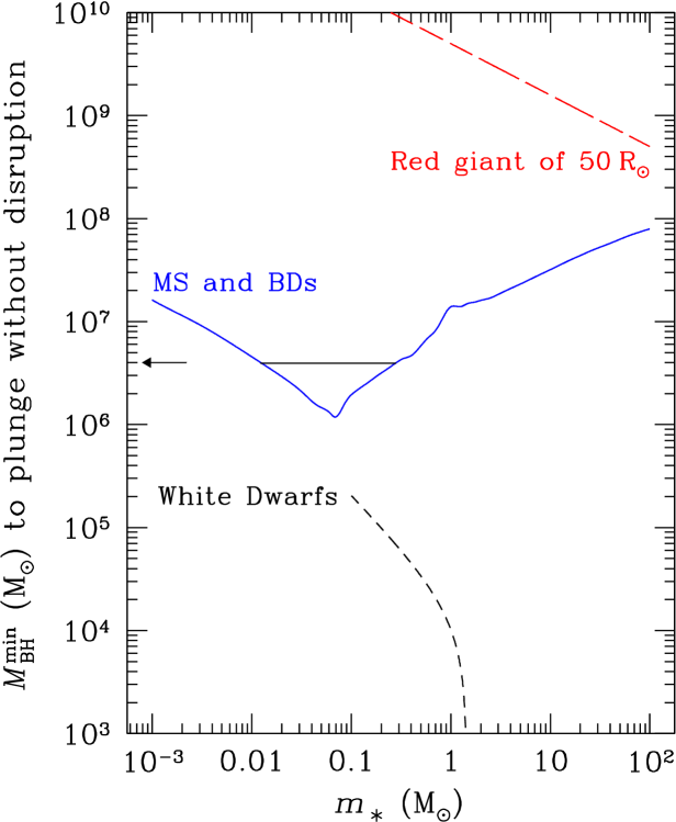
Figure 1: Minimum mass for a MBH for a given stellar object to plunge through the event horizon without a tidal disruption as a function of its mass $m_{\ast}$. For each different kind of stellar object — i.e., red giants, main sequence stars, and sub-stellar objects, we use realistic mass-ratio relations (see text). SgrA*, with a mass of about $\sim 4\times 10^{6}\,M_{\odot}$, is marked with an arrow, which indicates the range of masses of sub-stellar objects that might cross the event horizon without significant tidal stresses.

II Distribution around SgrA*

The quasi-steady solution for the distribution of stars around a MBH takes the form of an isotropic distribution function in energy space $f(E)\sim E^{\,p}$, which translates into $\rho(r)\sim r^{-\gamma}$ in terms of the stellar density $\rho$ (see Peebles (1972) and Bahcall and Wolf (1976), but also Gurevich (1964) for a similar solution for the distribution of electrons around a positively charged Coulomb centre). This solution has been confirmed a number of times using semi-analytical and numerical approaches; see, e.g., Shapiro and Marchant (1978); Marchant and Shapiro (1979, 1980); Shapiro and Teukolsky (1985); Freitag and Benz (2001); Amaro-Seoane et al. (2004); Preto et al. (2004). In particular, for our Galactic Centre, see the numerical work of (Baumgardt et al., 2018), which describes very well the observational data of (Gallego-Cano et al., 2018; Schödel et al., 2018). Therefore, we assume a power-law mass distribution for the stellar density,

$$\rho(r)=\rho_{0}\left(\frac{r}{r_{0}}\right)^{-\gamma},$$ (3)

with $\gamma$ the exponent value, and $\rho_{0}$ the stellar density at a characteristic radius $r_{0}$ of normalization. Since we are interested in power-law cusps, as we will discuss later, this can be chosen to be the influence radius, $r_{0}\equiv R_{\rm h}$, and is only valid for radii smaller than this value. The enclosed mass $M(r)$ at a certain radius $r$ can be estimated by solving the integral

$$M(r)=4\,\pi\int^{r}_{0}\rho(r^{\prime})\,r^{\prime 2}dr^{\prime},$$ (4)

so that, with the proviso that $\gamma<3$,

$$M(r)=\frac{4\,\pi}{3-\gamma}\,\rho_{0}\,r_{0}^{3}\left(\frac{r}{R_{\rm h}}\right)^{(3-\gamma)}.$$ (5)

Main sequence (MS) stars build a power-law distribution about the MBH, so that we can set $r_{0}=R_{\rm h}$ for them, the influence radius of the MBH at the Galactic Centre. Also, $M_{\rm BH}:=(4\,\pi)/(3-\gamma)\cdot\rho_{0}\,r_{0}^{3}$ is the mass of the MBH, we have

$$M(r)=M_{\rm BH}\left(\frac{r}{R_{\rm h}}\right)^{(3-\gamma)}$$ (6)

Assuming that the mean stellar mass $\bar{m}_{\ast}$ at the radii of interest is independent of the radius, the number of stars at a given radius $r$ is

$$N_{\ast}(r)=\frac{M(r)}{\bar{m}_{\ast}}=\frac{M_{\rm BH}}{\bar{m}_{\ast}}\left(\frac{r}{R_{\rm h}}\right)^{(3-\gamma)}$$ (7)

Hence, the number of a given sub-population with a number fraction $f_{\rm sub}$ of the stars at a radius $r$ can be calculated with

$$N_{\rm sub}(r)=f_{\rm sub}\frac{M_{\rm BH}}{\bar{m}_{\ast}}\left(\frac{r}{R_{\rm h}}\right)^{(3-\gamma)}.$$ (8)

We must take into account that by doing so we are implicitly assuming that light stars (or substellar objects, the main interest of this work) follow the same distribution as MS stars. In this approach, both the MS stars and the BDs are the light stellar component with their own power-law index, different to the power-law index of stellar-mass black holes, which build a more concentrated distribution around the MBH. A more realistic representation would require more than two different exponents, but then it would be very difficult to treat the problem analytically, as we do in this article. While until now we have used $\gamma$ as a generic exponent, from now on, we will use it only for the exponent of the stellar-mass black hole population (for historical reasons this has been the convention), and $\beta$ for the light star population, i.e. the BDs.

To derive $\bar{m}_{\ast}$ and $f_{\rm sub}$, we have to take into account that BDs have masses ranging from approximately $0.01-0.07\,M_{\odot}$ (which is actually a lower limit, since they can also have masses in the range $0.07-0.15\,M_{\odot}$ through the BD formation process, see Kroupa et al. (2013)) and have their own initial mass function (IMF), which is not well known-, but can be approximated by a single power law; see Eq. (4.55) of Kroupa et al. (2013), which is consistent with observational data of the inner galaxy (Wegg et al., 2017). The IMF we consider is the usual Kroupa broken power-law of the form $dN_{\ast}/dm_{\ast}\propto m_{\ast}^{-\alpha}$. We use the mass intervals $[0.01,\,0.07,\,0.5,\,150]\,\times M_{\odot}$ with $\alpha=0.3,\,1.3,\,2.3$, because the bulge may have had a top-heavy IMF; see (Bartko et al., 2010) and (Ballero et al., 2007) for some constraints on the top-heaviness in the bulge, althought it remains unknown if the IMF below $1\,M_{\odot}$ was different (Pavel Kroupa, personal communication). We hence introduce a discontinuity in this IMF to mimic the discontinuity between the sub-stellar (BDs) population and the stellar IMF at $0.07\,M_{\odot}$ (Fig. 4-23 of (Kroupa et al., 2013)). Assuming these values, we find that for the BDs, $f_{\rm sub}\sim 0.21$, and that the average stellar mass is $\bar{m}_{\ast}\sim 0.27\,M_{\odot}$. Taking into account that the influence radius of our MBH, SgrA*, is $R_{\rm h}\sim 3\,{\rm pc}$ (Schödel et al., 2014, 2018), and adopting the value $\beta=1.5$ (Bahcall and Wolf, 1977), we obtain that

$$N_{\rm BD}(r)\cong 6\times 10^{5}r_{\rm pc}^{1.5},$$ (9)

with $r_{\rm pc}$ the considered radius in pc. Therefore, at a distance of $10^{-3}\,{\rm pc}$, there should be around $\sim 20$ BD. This is the number of sources as a function of radius; however, the the phenomenon we are interested on— the formation, evolution and merger of an X-MRI with the central MBH— also represents a drain on these sources. In order to have a statistical picture of what we might expect at the Galactic Centre once LISA starts to gather data, we need to address the (relativistic) loss-cone problem of this scenario. This will also allow us to derive an event rate.

III Loudness

Assuming that one of these objects could indeed be in the relevant part of phase space and become a source, in order to assess whether these sources are interesting for LISA, we estimate in this section the signal-to-noise ratio (SNR). At a distance D given, an EMRI with a power emitted $\dot{E}$ and a rate of change of frequency $\dot{f}$, its characteristic amplitude $h_{\rm c}$ can be defined as $h_{\rm c}=\sqrt{(2\dot{E}/\dot{f})}/(\pi D)$ (Finn and Thorne, 2000). If we assume a perfect signal processing, the sky- and orientation-averaged SNR is given by (Finn and Thorne, 2000)

$$\left(\frac{S}{N}\right)^{2}=\frac{4}{\pi D^{2}}\int\frac{\dot{E}}{\dot{f}\,S_{h}^{SA}(f)}\frac{{\rm d}f}{f^{2}},$$ (10)

with $S_{h}^{SA}(f)\approx 5S_{h}(f)$ the noise spectral density of the detector. In the case of the EMRI problem, we need to sum the previous expression over each mode to obtain the total SNR², since the signal has multiple frequency components. In this article we consider quadrupolar gravitational radiation, and approach the orbit as a Keplerian ellipse with parameters that evolve slowly due to the emission of GWs, as presented in the work of (Peters, 1964). Following this approximation, we decompose the amplitude in a series of harmonics. For typical values relevant to this article, the n-th harmonic at a distance $D$ is given by

$$h_{n} =g(n,e)\frac{G^{2}\,M_{\rm BH}m_{\rm BD}}{D\,ac^{4}}$$

$$\simeq 10^{-18}g(n,e)\left(\frac{D}{8\,\mathrm{kpc}}\right)^{-1}\left(\frac{a}{10^{-3}\,\mathrm{pc}}\right)^{-1}$$

$$\left(\frac{M_{\rm BH}}{4\times 10^{6}\,M_{\odot}}\right)\left(\frac{m_{\rm BD}}{0.05\,M_{\odot}}\right).$$

In this equation, $g(n,\,e)$ is a function of the harmonic number $n$, and $e$ the eccentricity. Also, we note that the root mean square is considered to be averaged over the two polarizations and all directions. We hence consider the contribution of the different harmonics (see Eq. 2.1 of (Finn and Thorne, 2000) and Eq. 56 of Barack and Cutler (2004) for more details),

$$\left(\frac{S}{N}\right)^{2}_{n}=\int^{f_{n}(\rm t_{fin})}_{f_{n}(\rm t_{ini})}\left[\frac{h_{\rm c,\,n}(f_{n})}{h_{\rm det}(f_{n})}\right]^{2}{\frac{1}{f_{n}}\,d\left(\ln(f_{n})\right)}.$$ (11)

In this equation $f_{n}(t)$ is the (in principle redshifted, but irrelevant for the GC) frequency of the nth harmonic at time $t$ (with $f_{n}=n\cdot f_{\rm orb}$, $f_{\rm orb}$ being the orbital frequency, and we note that there are two differing orbital frequencies for an eccentric body, radial and azimuthal. In Barack and Cutler (2004) a compromise between the two is introduced.) and $h_{\rm c,\,n}(f_{n})$ the characteristic amplitude of the nth harmonic when the frequency associated to that component is $f_{n}$. Finally, $h_{\rm det}$ is the square root of the sensitivity curve of LISA and we note that $d\left(\ln(f_{n})\right)/f_{n}$ is simply $df_{n}$.

In Fig. (2) we give an example of an X-MRI of a given mass for the BD object at the GC. The curves are to be interpreted as the SNR that we would observe if we integrated for one year. Hence, at a given time in the X axis, the SNR is what we would obtain if we followed the source for one year-, i.e. if LISA could only operate for one year. We can see that from starting about $10^{7}~{}{\rm yrs}^{-1}$ before plunging through the event horizon, these sources already have SNR $>10$. If the sources were on their last year of inspiral when LISA starts to get data, the SNR would be as much as a few $10^{3}$ for the light BD in the left panel and $\sim 2\times 10^{4}$ for the larger one in the right panel. We note that our calculation of the SNR is in good agreement with the one done by (Barack and Cutler, 2004), which addressed extended stars of low mass undergoing tidal disruptions at the GC, and the more recent work of (Gourgoulhon et al., 2019), which focuses on circular orbits. In Fig. (3) we show the peak of the frequency emitted by the same systems.

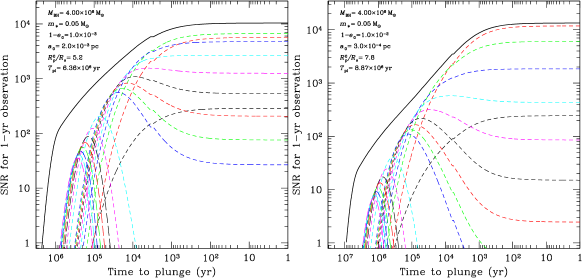
Figure 2: SNR obtained by LISA for a one-year observation for an X-MRI of mass $0.05\,M_{\odot}$ at the GC. At a given time, the curve shows the SNR we would get if we followed the X-MRI for one year. The mass of the MBH is set to $M_{\rm BH}=4\times 10^{6}M_{\odot}$, while the initial eccentricity to and semi-major axis are set to typical values. We show the initial pericentre distance in terms of the Schwarzschild radius of the MBH and the (initial) time for the star to plunge on to it under the assumption that it evolves only due to the loss of energy in the form of GWs, as approximated by (Peters, 1964). We show the contribution of the first 10 harmonics (displayed in different colours, and we note that we have used 1000 in the calculation of the SNR). The black, solid line corresponds to the total SNR and the red, dashed curve, to the second harmonic.

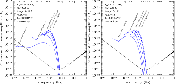
Figure 3: Peak of the gravitational wave frequency emitted by the X-MRI systems of Fig. (2). Each blue line is an isochrone made by selecting a given moment before the final plunge, shown as a dashed label, for the first 1000 harmonics (see text), although we only depict the first ten ones in each line, at the same time, with circles. The curves are an interpolation from the 1000 harmonics. Additionally, we show the corresponding pericentre distance $R_{\rm p}$ in units of the Schwarzchild radius $R_{\rm S}$ and the eccentricity. The time $T_{\rm pl}$ is the time to merge as calculated from the initial dynamical parameters of the binary, displayed at the top, left legend.

IV Event Rates

The event rate, i.e., the number of X-MRIs that successfully inspiral and cross the event horizon can be calculated by integrating in phase-space the number of sources from a critical radius $a_{\rm crit}$ down to a minimum distance, $a_{\rm min}$,

$$\dot{\Gamma}_{\rm X-MRI}\simeq\int^{a_{\rm crit}}_{a_{\rm min}}\frac{dn_{\rm BD}(a)}{T_{\rm rlx}(a)\,\ln{\left(\theta_{\rm lc}^{-2}\right)}}\,.$$ (12)

We do not need to care about the specific shape of the curve in the integral, because on the left of the LSO the integral will naturally vanish. To solve this integral, we need (1) $\theta_{\rm ls}$, the loss-cone angle (see e.g. Amaro-Seoane (2018c)), (2) $n_{\rm BD}(a)$ the number of BDs within a given semi-major axis $a$, (3) $T_{\rm rlx}(a)$ the relaxation time, and (4) $a_{\rm crit}$ and $a_{\rm min}$ the critical and minimum radii, which is the upper and lower limits of the integral.

IV.1 The loss-cone angle

The first quantity, (1) the loss-cone angle, can be estimated as (Alexander and Livio, 2001)

$$\theta_{\rm lc}\simeq\frac{1}{\sqrt{J_{\rm max}/J_{\rm lc}}}.$$ (13)

Using the same reference, we have that

$$J_{\rm lc}\simeq\frac{4\,G}{c}\,M_{\rm BH},\,J^{2}_{\rm max}=GM_{\rm BH}a,$$ (14)

so that we obtain the first quantity to solve the integral,

$$\theta^{2}_{\rm lc}\simeq\sqrt{\frac{8\,R_{\rm S}}{a}}.$$ (15)

IV.2 Number of sources within a given radius

Regarding the second quantity, (2) the number of BDs within a specific semi-major axis $a$, we have already estimated in the previous section how many BDs we might expect. Hence, the number of BDs within $a$ is

$$N_{\rm BD}(a)=f_{\rm sub}^{\rm BD}\cdot N^{\rm BD}_{0\,\textrm{MS}}\left(\frac{a}{R_{0}}\right)^{3-\beta}\,.$$ (16)

As discussed previously, $N^{\rm BD}_{0\,\textrm{MS}}$ is the total number of objects (main-sequence stars and substellar objects) within $R_{0}$, which we choose to be $R_{\rm h}$, and $f_{\rm sub}^{\rm BD}$ is the number fraction of BDs. In order to obtain the numerator in the integrand of Eq. (12), we differentiate the last equation and obtain the second quantity,

$$dn_{\rm BD}(a)=f_{\rm sub}^{\rm BD}\,(3-\beta)\frac{N^{\rm BD}_{0\,\textrm{MS}}}{R_{h}}\left(\frac{a}{R_{h}}\right)^{2-\beta}da\,.$$ (17)

IV.3 The relaxation time

We can calculate the third quantity, (3) the relaxation time, by approximating relaxation to be predominantly due to the population of stellar-mass black holes of mass $m_{\rm bh}$, which dominate the central densities (e.g. Amaro-Seoane (2018c)).

The relaxation time for a given distance which we take to be equal to the semi-major axis $a$ is

$$T_{\rm rlx}(a)=T_{0}\left(\frac{a}{R_{0}}\right)^{\gamma-3/2}\,,$$ (18)

with (Spitzer, 1987)

$$T_{0}\sim 0.3389\,\frac{\sigma_{0}^{3}}{\ln(\Lambda)\,G^{2}\,m_{\rm bh}^{2}\,n_{0}}\,,$$ (19)

and

$$n_{0} =\frac{3-\gamma}{4\pi}\frac{N_{0}}{R_{0}^{3}}$$ (20)

$$\sigma_{0}^{2} =\frac{1}{1+\gamma}\frac{GM_{\rm BH}}{R_{0}}.$$ (21)

In the previous equations $\ln(\Lambda)$ is the Coulomb logarithm, $G$ the gravitational constant, $\sigma_{0}$ the velocity dispersion, $R_{0}$ is the radius within which stellar-mass black holes dominate relaxation, and $N_{0}$ the number of stellar-mass black holes enclosed in $R_{0}$ which, in principle, can be smaller than the influence radius $R_{\rm h}$. Hence, Eq. (19) becomes

$$T_{0}\simeq\frac{4.26}{(3-\gamma)(1+\gamma)^{3/2}}\frac{\sqrt{R_{0}^{3}(GM_{\rm BH})^{-1}}}{\ln(\Lambda)\,N_{0}}\left(\frac{M_{\rm BH}}{m_{\rm bh}}\right)^{2}\,.$$ (22)

Before we carry on with the rest of quantities necessary to solve Eq. (12), we address two important points related to Eq. (18) and Eq. (22).

First, (i) in order to derive $R_{0}$ of Eq. (18), Eq. (20) and Eq. (21), we note that the relaxation rate is (see e.g. Amaro-Seoane (2018a))

$$\Gamma_{\rm rlx}=\frac{32}{\pi\,v_{\rm rel}^{3}}\ln(\Lambda)\,G^{2}\,n_{\ast}(m_{\rm bh}+m_{\ast})^{2}$$ (23)

This last equation expresses the “encounter relaxation time”, which depends on the characteristics of a peculiar class of encounter (see Amaro-Seoane (2018a)). I.e., for our purposes, a stellar-mass black hole of mass $m_{\rm bh}$ with a field MS star of mass $m_{\ast}$ with a local density $n_{\ast}$ and a relative velocity $v_{\rm rel}$. We can depict Eq. (23) thanks to the Monte-Carlo simulations of the Galactic Centre of Freitag et al. (2006). In their Fig. 10, right panel, they give the evolution of the density $\rho(r)$ profile for a standard Milky-Way nucleus after $1.05\times 10^{10}\,{\rm yrs}^{-1}$. From Eq.(23), $\Gamma_{\rm rlx}\propto n(r)\times m_{\rm obj}^{2}$, i.e. $\Gamma_{\rm rlx}\propto\rho(r)\times m_{\rm obj}$, with $m_{\rm obj}$ the mass of the object taken into consideration, a BD or a stellar-mass black hole. In Fig. (4) we show this quantity from the data of Freitag et al. (2006). We can see that from a distance of about $10\,{\rm pc}$, the relaxation rate is dominated by stellar-mass black holes. We note that the fact that within $\lessapprox 0.1~{}{\rm pc}$ the stellar-mass black holes have a tendency to follow a distribution which looks shallower than the one from the MS stars is due to a problem related to the resolution of the Monte Carlo simulations (M. Freitag, personal communication). On the other hand, we note that by assuming a pure power-law, as we are doing in our analytical approach, we are artificially increasing $T_{\rm rlx}$, since we are populating with more stellar-mass black holes the innermost radii. Therefore, the results that we will derive for Eq. (12) are to be regarded as a lower limit.

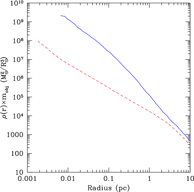
Figure 4: Relaxation rate for the Milky-Way model GN25 of Freitag et al. (2006) in $M_{\odot}^{2}$ per volume as a function of the radius from SgrA*. The red, dashed line corresponds to MS stars and the blue, solid line to stellar-mass black holes.

Secondly (ii), it must be noted that by assuming that relaxation is dominated by stellar-mass black holes, we are implying that relaxation can be added up individually from two mass groups, BDs and stellar-mass black holes, and that the contribution from BDs is negligible. In star cluster evolution, close to the central regions, energy equipartition is found only among the largest masses, and it progressively moves towards velocity equipartition at low masses (see e.g. Bianchini et al. (2016)). Hence, if the distribution function of mass and velocity is $f(m,\,v)$ with $v$ the velocity and $m$ the mass, and a moment of the change of velocities is of the form

$$<dv^{2}>=\int dv^{2}f(m,\,v)\,dm\,dv,$$

since energy equipartition among the low-mass object can be neglected, this last equation can be expressed as

$$<dv^{2}>=\sum_{m}n(m)\left(\int dv^{2}f(v)dv\right),$$

with $n(m)$ the density of stars of mass $m$. This has two important implications. First, we expect BDs to actually be close to the centre and, secondly, since the mass of the BD population is only a small contribution to the relaxation produced by stellar-mass black holes, we ignore their contribution in the calculations related to relaxational processes.

IV.4 The critical and minimum radii

We now need to calcuate the only remaining quantities, (4) the critical and the minimum semi-major axis. The critical radius, the upper limit of integral Eq. (12), can be derived by taking into account its definition. This is the semi-major axis at which the threshold curve which separates the dynamics- and GW-regime merges with the LSO curve. First, we equate the relaxation time to the inspiral timescale for a binary made from the MBH and a BD,

$$T_{\rm rlx,\,peri}=C\,T_{\rm GW}(a,\,e)$$ (24)

In this equation, $T_{\rm rlx,\,peri}$ is the relaxation time at pericentre, i.e., $T_{\rm rlx,\,peri}:=T_{\rm rlx}(a)\times(1-e)$ (Amaro-Seoane, 2018c), and $C\sim 1$. Since at the radii of interest the driving species in relaxation is that of stellar-mass black holes, the mass that matters in the expression of $T_{\rm rlx,\,peri}$ is $m_{\rm bh}$. However, we are interested in the inspiral of a BD into the MBH, and hence the mass which is relevant for the right-hand side is $m_{\rm BD}$. We assume here that $e\sim 1$, which is the characteristic eccentricity of EMRIs when they form (Amaro-Seoane, 2018c), so that the function $f(e)$ which appears in $T_{\rm GW}(a,\,e)$, Peters (1964)-, can be approximated as $f(e)=425/(768\,\sqrt{2})$.

We assume Newtonian parabolic orbits because BDs will have semi-major axes much larger than their pericentre distance. We hence equate the Newtonian value of the pericentre distance of the last stable parabolic orbit around the massive black hole (Shapiro and Teukolsky, 1983) to the pericentre distance,

$$\frac{8\,G{M}_{\rm BH}}{c^{2}}=a\,(1-e)\cal{W}(\iota,\,{\rm s}).$$ (25)

In this equation, we have multiplied the right-hand side by the function $\cal{W}(\iota,\,{\rm s})$, which takes into account the impact of the asymmetry between prograde and retrograde orbits on the location of the LSO for a Kerr MBH with respect to the Schwarzschild case (at a distance $4\,R_{\rm S}$) Amaro-Seoane et al. (2013). This function depends on the inclination of the orbit, $\iota$ and the magnitude of the spin of the MBH, $\rm{s}$.

Therefore, we obtain that

$$T_{\rm GW}(a,\,e)\sim\sqrt{2}\,\frac{24}{85}\frac{c^{5}}{G^{3}}\frac{a^{4}\,\left(1-e\right)^{7/2}}{m_{\rm BD}\,M_{\rm BH}^{2}}.$$ (26)

From Eqs. (24), (18) and (22), we can obtain the relation between $a$ and $e$, the threshold curve between the dynamics-dominated regime and the gravitational-wave one, which we use for the dashed, red curve of Fig.(5),

$$\left(1-e\right)^{5/2} =\frac{4.26}{(3-\gamma)(1+\gamma)^{3/2}}\frac{85}{24}\frac{1}{\sqrt{2}\,c^{5}}\frac{G^{\,5/2}}{\ln(\Lambda)}$$

$$\frac{M_{\rm BH}^{7/2}}{N_{0}}\frac{m_{\rm BD}}{m_{\rm bh}}R_{0}^{3-\gamma}a^{\gamma-11/2}$$ (27)

As before, $R_{0}$ is a characteristic radius, within which relaxation is dominated by stellar-mass black holes, and $N_{0}$ is the number of them contained in that radius. Because of the explanation we gave before about stellar-mass black holes dominating relaxation, we choose now to set this radius also to the influence radius, $R_{\rm h}$, as we did with the normalisation of the BDs and MS stars.

We can see that the threshold for these binaries to decouple from the stellar system is around a distance of $2.5\times 10^{-3}\,{\rm pc}$. Indeed, solving the same equations for $a_{\rm crit}$, we have that

$$a_{\rm crit} =\epsilon\,R_{0}\times$$

$$\times\left[{\cal W}(\iota,\,{\rm s})^{5/2}\,N_{0}\ln(\Lambda)\left(\frac{M_{\rm BH}}{m_{\rm BD}}\right)\left(\frac{M_{\rm BH}}{m_{\rm bh}}\right)^{-2}\right]^{\frac{1}{\gamma-3}},$$ (28)

where we have defined

$$\epsilon:=\left[\frac{C}{4.26}\frac{6144}{85}(3-\gamma)(1+\gamma)^{3/2}\right]^{\frac{1}{\gamma-3}}.$$ (29)

Adopting $\gamma=1.75$, $R_{0}=R_{\rm h}=3\,{\rm pc}$, we have that BDs have the following $a_{\rm crit}$ at the GC

$$a_{\rm crit} \sim 2.89\times 10^{-3}\,{\rm pc}\,{\cal W}(\iota,\,{\rm s})^{-2}\times$$

$$\left(\frac{M_{\rm BH}}{4\cdot 10^{6}M_{\odot}}\right)^{4/5}\left(\frac{m_{\rm BD}}{0.05M_{\odot}}\right)^{4/5}\times$$

$$\left(\frac{m_{\rm bh}}{10M_{\odot}}\right)^{-8/5}\left(\frac{N_{0}}{10^{4}}\right)^{-4/5}\left(\frac{ln(\Lambda)}{12}\right)^{-4/5}.$$ (30)

In Fig. (5) we depict this threshold for the same values in phase-space for the values of $\gamma$ and $\beta$ of (Bahcall and Wolf, 1977). We note that our analytical model does not take into account the fact that dynamical friction will bring in more stellar-mass black holes within the influence radius. For instance, the Milky-Way models of Freitag et al. (2006) find $\sim 2\times 10^{4}$ stellar-mass black holes at a distance of $R=1\,\textrm{pc}$. However, since the dependency of $a_{\rm crit}$ on $N_{0}$ has an exponent of $4/5$, the difference is small. This is also true for the dependency on $m_{\rm BD}$, with e.g. $a_{\rm crit}\sim 5\times 10^{-3}\,{\rm pc}\,{\cal W}(\iota,\,{\rm s})^{-2}$ for $m_{\rm BD}=0.1\,M_{\odot}$.

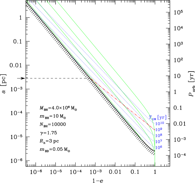
Figure 5: Definition of the critical radius $a_{\rm crit}$ in the phase space in the semi-major axis (in parsecs) and eccentricity plane, $a$ – $(1-e)$, for the inspiral of a BD of mass $m_{\rm BD}=0.05\,M_{\odot}$, into a MBH of mass $4\times 10^{6}\,M_{\odot}$. The dashed, blue lines are isochrones depicting the inspiral time $T_{\rm GW}$ in years of the binary, were this to evolve only due to the emission of gravitational radiation, as estimated in the approximation of Peters and Mathews (1963). When a system crosses one of the isochrones, it will inspiral in a time as shown by the corresponding curves. The green curves show the relation between $a$ and $e$ as estimated in the work of Peters (1964), again under the same assumption. The red, dashed line gives the threshold for two different regimes in the evolution of the binary, as derived in Eq. (27). Above this line the binary evolves due to two-body relaxation, while below the curve the driving mechanism is the emission of GWs. The solid, black line crossing the figure from the top left to the bottom right is the last stable orbit (LSO) for a Schwarzschild MBH of that mass. The conjunction of the red line with the LSO defines the critical semi-major axis $a_{\rm crit}$, which is shown with an arrow on the y-axis.

The minimum radius is the distance within which we expect to have at least one object to start the integration. This can be derived from Eq. (8) taking into account that $N^{\rm BD}_{0\,\textrm{MS}}={M_{\rm BH}}/{\bar{m}_{\ast}}$. Hence,

$$a_{\rm min}\simeq 1.65\times 10^{-5}\,\textrm{pc}\,f_{\ast,\,\textrm{sub}}^{-2/3}\left(\frac{R_{\rm h}}{1\,\textrm{pc}}\right),$$ (31)

with $f_{\ast,\,\textrm{sub}}$ the fraction of substellar objects or stars taken into consideration, and adopting $\beta=3/2$.

With all of the quantities defined, we substitute them into Eq. (12) and find that the integral has as solution

$$\dot{\Gamma}_{\rm X-MRI}=\frac{3-\beta}{2\,\lambda}\frac{N^{\rm BD}_{0\,\textrm{MS}}}{T_{0}\,R_{\rm h}^{\lambda}}f_{\rm sub}^{\rm BD}\times$$

$$\left\{a_{\rm crit}^{\lambda}\left[\ln(\Lambda_{\rm crit})-\frac{1}{\lambda}\right]-a_{\rm min}^{\lambda}\left[\ln(\Lambda_{\rm min})-\frac{1}{\lambda}\right]\right\},$$ (32)

where we have introduced

$$\lambda :=9/2-\beta-\gamma$$

$$\Lambda_{\rm crit} :=\left(\frac{a_{\rm crit}}{8\,R_{\rm S}}\right)$$

$$\Lambda_{\rm min} :=\left(\frac{a_{\rm min}}{8\,R_{\rm S}}\right).$$ (33)

IV.5 Results for two classical examples

We now give two examples for the values of the critical parameters for two different solutions of the power-laws. For historical reasons, we use the values derived by Bahcall and Wolf (1977), but note that the values found by the authors, $\gamma=7/4$ and $\beta\rightarrow 3/2$ are a (heuristically) generalised solution of their earlier work Bahcall and Wolf (1976) that only depends on the mass ratio of the two different populations. While this solution is mathematically correct, it assumes a stellar population in which 50% of all stars are stellar-mass black holes. We refer to this model using the sub- and superscript “BW”.

We then give a more accurate value, which corresponds to more appropriate number fractions. This translates into a more efficient diffusion, as noted by Alexander and Hopman (2009) and Preto and Amaro-Seoane (2010). In particular, $\gamma=2$ and the population of stars with lighter masses $\beta=3/4$, as found with the direct-summation $N-$body simulations of Preto and Amaro-Seoane (2010) (see also Amaro-Seoane and Preto (2011)). The notation in this case is “SMS” (i.e. strong-mass segregation, a term coined by Tal Alexander).

For legibility, we now introduce the following notation for standard values of normalisation,

$$\tilde{\Lambda} :=\left(\frac{\ln(\Lambda)}{13}\right),~{}\tilde{N}_{0}:=\left(\frac{N_{0}}{12000}\right)$$

$$\tilde{R}_{0} :=\left(\frac{R_{\rm h}}{1\textrm{pc}}\right),~{}\tilde{m}_{\rm BD}:=\left(\frac{m_{\rm BD}}{0.05\,M_{\odot}}\right).$$ (34)

We have chosen the value of $\tilde{\Lambda}$ based on the fact that the galactic nucleus is a non self-gravitating system, so that $\ln(\Lambda)\simeq\ln(M_{\rm BH}/m_{\rm bh})\sim 12.9$ (see e.g. Amaro-Seoane (2018a)).

The BW case leads to the following results for the critical radius and the normalization timescale $T_{0}$,

$$a^{\rm BW}_{\rm crit} \sim 8\times 10^{-4}\,\textrm{pc}\,{\cal W}(\iota,\,{\rm s})\tilde{R}_{0}\tilde{N}_{0}^{-4/5}\tilde{\Lambda}^{-4/5}\tilde{m}_{\rm BD}^{4/5}$$

$$T^{\rm BW}_{0} \sim 10.34\times 10^{9}\,\textrm{yrs}\,\tilde{R}_{0}^{3/2}\tilde{N}_{0}^{-1}\tilde{\Lambda}^{-1}.$$ (35)

Hence, the BW event rate is

$$\dot{\Gamma}_{\rm BW} \sim 1.8\times 10^{-4}\,\textrm{yrs}^{-1}\tilde{N}_{0}\,\tilde{\Lambda}\,\tilde{R}_{0}^{-11/4}\times$$

$$\Bigg{\{}1.34\times 10^{-4}\tilde{R}_{0}^{5/4}\tilde{N}_{0}^{-1}\tilde{\Lambda}^{-1}\tilde{m}_{\rm BD}\,{\cal W}(\iota,\,{\rm s})\times$$

$$\left[\ln\left(262\,\tilde{R}_{0}\,\tilde{N}_{0}^{-4/5}\tilde{\Lambda}^{-4/5}\tilde{m}_{\rm BD}^{4/5}\,{\cal W}(\iota,\,{\rm s})^{-2}\right)-\frac{4}{5}\right]-$$

$$6.86\times 10^{-25/4}\tilde{R}_{0}^{5/4}\times\left[\ln\left(15.22\,\tilde{R}_{0}\right)-\frac{4}{5}\right]\Bigg{\}}.$$ (36)

The same quantities calculated for the SMS case are,

$$a^{\rm SMS}_{\rm crit}\sim 1.4\times 10^{-4}\,\textrm{pc}\,{\cal W}(\iota,\,{\rm s})^{-5/4}\tilde{R}_{0}\tilde{N}_{0}^{-1}\tilde{\Lambda}^{-1}\tilde{m}_{\rm BD}$$

$$T^{\rm SMS}_{0}\sim 1.13\times 10^{9}\,\textrm{yrs}\,\tilde{R}_{0}^{3/2}\tilde{N}_{0}^{-1}\tilde{\Lambda}^{-1}.$$ (37)

With these, the event SMS rate can be derived to be

$$\dot{\Gamma}_{\rm SMS} \sim 2.3\times 10^{-3}\,\textrm{yrs}^{-1}\tilde{R}_{0}^{-5/2}\tilde{N}_{0}\tilde{\Lambda}\times$$

$$\Bigg{\{}1.4\times 10^{-4}\tilde{R}_{0}\,\tilde{N}_{0}^{-1}\tilde{\Lambda}^{-1}\tilde{m}_{\rm BD}\,{\cal W}(\iota,\,{\rm s})^{-5/2}\times$$

$$\left[\ln\left(46\,\tilde{R}_{0}\,\tilde{N}_{0}^{-1}\tilde{\Lambda}^{-1}\tilde{m}_{\rm BD}\,{\cal W}(\iota,\,{\rm s})^{-5/2}\right)-1\right]-$$

$$4.67\times 10^{-7}\tilde{R}_{0}\times\left[\ln\left(15.24\,\tilde{R}_{0}\right)-1\right]\Bigg{\}}.$$ (38)

In Fig. (6) we show a few examples for the SMS cases, including one for the BW. The rates typically are about $10^{-5}\,\textrm{yr}^{-1}$ for the SMS case and one order of magnitude less for the less realistic BW scenario.

Figure 6: Number of sources per year at the GC that successfully inspiral towards SgrA* as a function of the spin of the MBH and the inclination of the orbit $\iota$ in rad, for typical values of the mass of the BD. We include as well two different values of the influence radius, which is the value we have chosen for the normalization radius $R_{0}$, of $1\,\textrm{pc}$ (for being a traditional value in the related literature) and of $3\,\textrm{pc}$ (according to more recent observations, see (Schödel et al., 2014, 2018)). We show three characteristic combinations for the SMS scenario and one for the less realistic BW case.

IV.6 A check of our model

Thanks to Eqs. (32, 28, 22), we can evaluate our results by simplyfing our analysis to the specific case of stellar-mass black holes. We can easily re-calculate the previous equations for this kind of stellar objects and define the quantity $\tilde{m}_{\rm bh}:=m_{\rm bh}/(10\,M_{\odot})$ by analogy with the previous section. We find that the event rate for the BW case is

$$\dot{\Gamma}_{\rm BW,\,bh} \sim 2.63\times 10^{-6}\,\textrm{yrs}^{-1}\tilde{N}_{0}\,\tilde{\Lambda}\,\tilde{R}_{0}^{-5/2}\,\tilde{m}_{\rm bh}^{2}\times$$

$$\Bigg{\{}5\times 10^{-2}\tilde{R}_{0}\tilde{N}_{0}^{-4/5}\tilde{\Lambda}^{-4/5}\tilde{m}_{\rm bh}^{4/5}\,{\cal W}(\iota,\,{\rm s})^{-2}\times$$

$$\left[\ln\left(16318\,\tilde{R}_{0}\,\tilde{N}_{0}^{-4/5}\tilde{\Lambda}^{-4/5}\tilde{m}_{\rm bh}^{4/5}\,{\cal W}(\iota,\,{\rm s})^{-2}\right)-1\right]\times$$

$$2\times 10^{-3}\tilde{R}_{0}\times\left[\ln\left(618\,\tilde{R}_{0}\right)-1\right]\Bigg{\}}.$$ (39)

For the standard value of $\tilde{m}_{\rm bh}=1$ (and the rest of parameters set to unity), we recover the usual rate of $\dot{\Gamma}_{\rm BW,\,bh}\sim 10^{-6}\,\textrm{yr}^{-1}$ (see e.g. Amaro-Seoane, 2018a, and references therein). For more massive stellar-mass black holes, in particular for $\tilde{m}_{\rm bh}=4$ (i.e. $m_{\rm bh}=40\,M_{\odot}$), which is the scenario recently proposed by (Emami and Loeb, 2019) for EMRIs at the GC, we find a slightly enhanced rate, but still negligible, $\dot{\Gamma}_{\rm BW,\,bh}\sim 6.2\times 10^{-5}\,\textrm{yr}^{-1}$.

For completness, we give now the case corresponding to SMS,

$$\dot{\Gamma}_{\rm SMS,\,bh} \sim 1.92\times 10^{-6}\,\textrm{yrs}^{-1}\tilde{N}_{0}\,\tilde{\Lambda}\,\tilde{R}_{0}^{-2}\,\tilde{m}_{\rm bh}^{2}\times$$

$$\Bigg{\{}1.6\times 10^{-1}\tilde{R}_{0}^{1/2}\tilde{N}_{0}^{-1/2}\tilde{\Lambda}^{-1/2}\tilde{m}_{\rm bh}^{1/2}\,{\cal W}(\iota,\,{\rm s})^{-5/4}\times$$

$$\left[\ln\left(9138\,\tilde{R}_{0}\,\tilde{N}_{0}^{-1}\tilde{\Lambda}^{-1}\tilde{m}_{\rm bh}\,{\cal W}(\iota,\,{\rm s})^{-5/2}\right)-2\right]-$$

$$4\times 10^{-2}\tilde{R}_{0}^{1/2}\times\left[\ln\left(618\,\tilde{R}_{0}\right)-2\right]\Bigg{\}}.$$ (40)

V Number of sources in band

Contrary to EMRIs, which are more massive, X-MRIs spend a long time in band, because they undergo $\sim\,10^{8}$ cycles before they cross the event horizon of the MBH. In Fig. (2) we see that they can spend as much as $\sim 10^{6}\,{\rm yr^{-1}}$ with a SNR $>10$. Since the event rate at the GC is of about $\dot{\Gamma}_{\rm X-MRI}\sim 10^{-5}\,{\rm yr}^{-1}$, we could naively argue that at any given time there should be $\sim 10\times\dot{\Gamma}_{\rm X-MRI}$ sources at different frequencies. These would have different SNRs, from tens to a few $10^{3}$ or even $\gtrsim 10^{4}$, depending on their mass.

However, not all of these objects will be successful X-MRIs, because their semi-major axis must be below a threshold value, which we henceforth call $a_{\rm band}$. To derive this value and, therefore, the number of sources at any given time, we need to evaluate the number of sources $N$ at any given semi-major axis $a$; i.e. we need to assess the (line) density function

$$g=\frac{dN}{da}$$ (41)

as a function of $a$. In Fig. (7) we depict an illustrative shape of $g$. Because of the slow diffusion, $g$ must have larger values at larger values of $a$. However, the number of sources sweeping the different range of values for $a$ is constant, so that $\Delta N(t=\Delta t)=\Delta N(t=0)$. This is equivalent to

Figure 7: Density of sources $g=dN/da$ as a function of $a$. Sources come from larger values of $a$, up to a maximum value at $a_{\rm max}$ —which is equivalent to $a_{\rm crit}$— and diffuse towards lower values-, down to a minimum $a_{\rm min}$. Sources with semi-major axis values above $a_{\rm band}$ emit GWs but at too low frequencies for detection. Those that cross the threshold value are in band. Sources above $a_{\rm break}$ have large eccentricities, while sources below it can be regarded as circular. In the text we derive the amount of sources in the regimes marked as ${\rm I}$ (with semi-major axis values between $a_{\rm min}$ and $a_{\rm break}$), ${\rm II}$ (between $a_{\rm break}$ and $a_{\rm band}$) and ${\rm III}$ (between $a_{\rm band}$ and $a_{\rm max}$).

$$\Delta t\left(v_{r}g_{r}-v_{l}g_{l}\right)=-\left(g(\Delta t)\Delta a-g(0)\Delta a\right),$$ (42)

where $v_{l}$, $g_{l}$ (and $v_{r}$, $g_{r}$) are respectively the values of the velocity and density function of the left (right)-, dashed line of Fig. (7). $g(0)$ is the density function at time $t=0$- and $g(\Delta t)$ after a time $\Delta t$, where the negative sign accounts for the fact that we are losing sources when crossing $a_{\rm min}$. Therefore,

$$\frac{v_{r}g_{r}-v_{l}g_{l}}{\Delta a}=-\frac{g(\Delta t)-g(0)}{\Delta t}.$$ (43)

In the limit $\Delta t\to 0$, this can be written as the continuity equation

$$\frac{\partial}{\partial a}\left(\dot{a}(a,\,e)g\right)+\frac{\partial g}{\partial t}=0,$$ (44)

where $\dot{a}(a,\,e)$ is the velocity, and it is a function of the semi-major axis $a$ and the eccentricity $e$. Its explicit form can be found in Peters (1964) in the approximation of Keplerian ellipses,

$$\dot{a}(a,\,e) =-\frac{64}{5}\frac{G^{3}\,M_{\rm BH}m_{\rm BD}(M_{\rm BH}+m_{\rm BD})}{c^{5}a^{3}(1-e^{2})^{7/2}}$$

$$\left(1+\frac{73}{24}e^{2}+\frac{37}{96}e^{4}\right),$$ (45)

Eq. (44) states that the rate at which sources enter the range of semi-major axis values is equal to the rate of sources leaving the system plus their accumulation. Since the density function does not vary in time, the right term vanishes. After integrating we obtain

$$\dot{a}(a,\,e)\,g=K,$$ (46)

with K a constant. In Fig. (7) we display a representative illustration of $a_{\rm band}$. The total number of sources is the amount of inspiraling BDs we derived in Sec. (IV), and are comprised between the values $a_{\rm max}$ and $a_{\rm min}$, so that all we need to do is to obtain the relative occupation fractions in the two areas to derive the number of sources detectable by LISA, i.e., those with semi-major axis between $a_{\rm band}$ and $a_{\rm min}$.

From Eqs. (41, 46), we have that

$$\frac{dN}{da}=\frac{K}{\dot{a}(a,\,e)}.$$ (47)

In order to integrate this function, we must distinguish two different regimes. Those X-MRIs with semi-major axis values above a threshold $a_{\rm break}$ still have a significant amount of eccentricity, while for lower values of the semi-major axis, the systems will be circular, or close to circular. We first address the eccentric regime. In Eq. (45) we now use the fact that the pericentre distance is $r_{p}=a(1-e)$. Therefore,

$$dN=Z(e)r_{p}^{7/2}a^{-1/2}da,$$ (48)

where we have introduced

$$Z(e)\equiv-\frac{5K}{64}\frac{c^{5}}{G^{3}}\frac{L(e)}{M_{\rm BH}m_{\rm BD}(M_{\rm BH}+m_{\rm BD})},$$ (49)

and

$$L(e):=\frac{\left(1-e\right)^{7/2}}{\left(1+\frac{73}{24}e^{2}+\frac{37}{96}e^{4}\right)}.$$ (50)

Since we are considering high values of eccentricity, $r_{p}$ is constant to first order (as can be seen in Fig. (3)) and can be taken out of the integral. In addition, $e\sim 1$ so that L(e) is constant and can also be taken out of the integral. Therefore, the number of sources between $a_{\rm max}$ and $a_{\rm break}$ is

$$\frac{dN}{da}\Big{|}_{a>a_{\rm break}}=\frac{dN}{da}\Big{|}_{a_{\rm break}}\left(\frac{a}{a_{\rm break}}\right)^{-1/2},$$ (51)

where we have normalized the distribution to $a_{\rm break}$. Integrating,

$$N(a>a_{\rm break}) =2\times a_{\rm break}\frac{dN}{da}\Big{|}_{a_{\rm break}}$$

$$\left[\left(\frac{a}{a_{\rm break}}\right)^{1/2}\right]_{a_{\rm break}}^{a_{\rm max}}.$$ (52)

For $a<a_{\rm break}$, we need to take into account that $e\sim 0$ in Eq.(45), so that

$$\frac{dN}{da}\Big{|}_{a<a_{\rm break}}=\frac{dN}{da}\Big{|}_{a_{\rm break}}\left(\frac{a}{a_{\rm break}}\right)^{3},$$ (53)

and, as in Eq. (51) we have normalized to the conjunction, $a_{\rm break}$. Therefore,

$$N(a<a_{\rm break}) =\frac{1}{4}\times a_{\rm break}\frac{dN}{da}\Big{|}_{a_{\rm break}}$$

$$\left[\left(\frac{a}{a_{\rm break}}\right)^{4}\right]_{a_{\rm break}}^{a_{\rm min}}.$$ (54)

By using Eq. (51), we obtain the ratios for the number of sources in ${\rm II}$ and ${\rm III}$ of Fig. (7),

$$\frac{N_{\rm II}}{N_{\rm III}}=\frac{a_{\rm band}^{1/2}-a_{\rm break}^{1/2}}{a_{\rm max}^{1/2}-a_{\rm band}^{1/2}}.$$ (55)

Likewise, by using Eqs. (51) and (54), we can obtain the ratio of sources between the region ${\rm I}$ (i.e., $N(a<a_{\rm break})$) and ${\rm II}+{\rm III}$ (i.e., $N(a>a_{\rm break})$),

$$\frac{N_{\rm I}}{N_{\rm II}+N_{\rm III}}=\frac{1}{8}\times\frac{1-\left(a_{\rm min}/a_{\rm break}\right)^{4}}{\left(a_{\rm max}/a_{\rm break}\right)^{1/2}-1}.$$ (56)

Finally, as we have discussed at the beginning of this section, we know that the total amount of sources in ${\rm I}$, ${\rm II}$ is Eq. (32) multiplied by the typical lifetime of these sources at a given eccentricity with a minimum SNR of 10, $T\left(a_{\rm max},e\right)\sim 2\times 10^{6}~{}{\rm yr}^{-1}$,

$$N_{\rm I}+N_{\rm II}=\dot{\Gamma}_{\rm X-MRI}\times T\left(a_{\rm max},e\right).$$ (57)

The plunge radius is $a_{\rm min}=2\times R_{\rm S}\sim 7.67\times 10^{-7}~{}{\rm pc}$. From Fig. (3), we see that a representative value of $a_{\rm break}\sim 4R_{\rm S}\sim 1.53\times 10^{-6}~{}{\rm pc}$. The value of $a_{\rm max}$ is given by Eq. (30), and a representative value of $a_{\rm band}$ with SNR=$10$ can be directly read from Fig. (3). Therefore, we obtain that

$$N_{\rm I} \sim 5$$

$$N_{\rm II} \sim 15.$$ (58)

We note that these values fluctuate by a multiplying factor of a few depending on the location of $a_{\rm band}$, which depends on the initial eccentricity of the source.

VI Conclusions

Brown dwarfs can inspiral in our Galactic Centre on to SgrA* via the emission of gravitational waves without suffering significant tidal stresses.

Because they have a mass ratio of $q\sim 10^{8}$, the time these systems spend in the LISA band is very long, since the number of times they revolve around the MBH is proportional to $q$. These systems, which we call X-MRIs, start to accumulate a signal-to-noise ratio of SNR=$10$ some $\sim 2\times 10^{6}~{}{\rm yrs}$ before the final plunge through the event horizon. At $10^{5}~{}{\rm yrs}$ before the merger, they achieve typically SNR $\sim{\rm few~{}}10^{2}$, and achieve values as high as SNR $\sim~{}10^{4}$ a thousand yrs before the plunge. Since SNR is inversely proportional to the distance of the source, these systems are also detectable in nearby galaxies-, or dwarf satellite galaxies, with the proviso that the MBH is in the range of masses of detection, such as Messier 32. For a MBH mass of $M_{\rm BH}=10^{6}\,M_{\odot}$ and $m_{\rm BD}=0.05\,M_{\odot}$, X-MRIs are detectable out to 50 Mpc with an SNR $=10$ 200 yrs before plunge.

A statistical treatment of the distribution of orbits in phase space which takes into account the asymmetry of the amount of pro- and retrograde orbits on the location of the LSO yields that every $\sim 10^{5}~{}{\rm yrs}$ one of these objects should cross the event horizon of SgrA*. The number of X-MRIs in band however is much larger. We have checked the results of our derivation by simplyfying it to a single stellar mass species, the case of stellar-mass black holes, and recover the usual results of the literature that the event rates per year are negligible in our GC, of $\sim 10^{-6}$, even if the mass of the stellar-mass black holes is set to $40\,M_{\odot}$.

These potential sources evolve extremely slowly, as compared to stellar-mass black hole EMRIs. By analysing the line density function in phase space, we derive that there are about $15$ X-MRIs at low frequencies with high eccentricities and associated SNRs of $\simeq~{}{\rm a~{}few~{}}100$, and about $5$, at higher frequencies, i.e. at very high SNRs (from ${\rm a~{}few~{}}100$ up to $2\times 10^{4}$), in circular-, or almost circular orbits. These numbers can be enhanced by a multiplyin factor of a few depending on the eccentricity of the sources when they form.

The higher the SNR, the faster X-MRIs evolve in frequency. However, even if it is less likely that LISA will observe an X-MRI of SNR $20,000$ as compared to one of a few $100$, the very loud systems live in band for as much as a few thousand years. A SNR of a few $100$ could already be problematic in the detection of a binary of SMBHs, and an X-MRI with SNR of a few $1000$ could bury the signal. Moreover, since X-MRIs can be detected for very long periodes of time with a high eccentricity, this will be a challenge from the point of view of data analysis, as compared to regular EMRIs. The values we have adopted to derive these results are conservative, so that one should take into account that X-MRIs might pose a problem if not in the detection of MBH binaries, then in their parameter extraction.

Also, we are artificially decreasing the event rate because we are limited in our analytical approach to pure power-laws. In numerical simulations the power-law decreases as one approaches the innermost radii. By populating this region with more stellar-mass black holes, we are artificially increasing $T_{\rm rlx}$, and hence decreasing the event rate, as it can be seen in Eq. (12). A more realistic approach should lead to an enhanced event rate, and therefore to more sources in band.

X-MRIs are interesting because backreaction depends on the mass ratio, which means that at $q\sim 10^{8}$, these systems are closer to a geodesic than EMRIs formed with larger $q$. This means that approximations in the calculation of the orbit are closer to the actual inspiral, and hence easier to model. A consequence is that it should not be difficult to separate X-MRIs signals from (potentially) weaker ones, such as binaries of MBHs. Because they can reach very large SNRs, and evolve very slowly in frequency, the parameter extraction can be done in detail. Contrary to EMRIs, X-MRIs can be regarded as monochromatic sources for space-borne detectors. To map spacetime around supermassive black holes in a fashion similar to EMRIs, a certain amount of different X-MRIs would be required with different parameters such as semi-major axes and inclinations. A detailed parameter study such as the role of phase accuracy in the waveform that can be achieved thanks to the high SNR is out of the scope of this paper, and will be presented in a separate study.

References

- Kormendy and Ho (2013) J. Kormendy and L. C. Ho, ARA&A 51, 511 (2013), arXiv:1304.7762 [astro-ph.CO] .
- Mezcua (2017) M. Mezcua, International Journal of Modern Physics D 26, 1730021 (2017), arXiv:1705.09667 .
- (3) N. Lützgendorf, M. Kissler-Patig, N. Neumayer, H. Baumgardt, E. Noyola, P. T. de Zeeuw, K. Gebhardt, B. Jalali, and A. Feldmeier, .
- Amaro-Seoane et al. (2017) P. Amaro-Seoane, H. Audley, S. Babak, J. Baker, E. Barausse, P. Bender, E. Berti, P. Binetruy, M. Born, D. Bortoluzzi, J. Camp, C. Caprini, V. Cardoso, M. Colpi, J. Conklin, N. Cornish, C. Cutler, K. Danzmann, R. Dolesi, L. Ferraioli, V. Ferroni, E. Fitzsimons, J. Gair, L. Gesa Bote, D. Giardini, F. Gibert, C. Grimani, H. Halloin, G. Heinzel, T. Hertog, M. Hewitson, K. Holley-Bockelmann, D. Hollington, M. Hueller, H. Inchauspe, P. Jetzer, N. Karnesis, C. Killow, A. Klein, B. Klipstein, N. Korsakova, S. L. Larson, J. Livas, I. Lloro, N. Man, D. Mance, J. Martino, I. Mateos, K. McKenzie, S. T. McWilliams, C. Miller, G. Mueller, G. Nardini, G. Nelemans, M. Nofrarias, A. Petiteau, P. Pivato, E. Plagnol, E. Porter, J. Reiche, D. Robertson, N. Robertson, E. Rossi, G. Russano, B. Schutz, A. Sesana, D. Shoemaker, J. Slutsky, C. F. Sopuerta, T. Sumner, N. Tamanini, I. Thorpe, M. Troebs, M. Vallisneri, A. Vecchio, D. Vetrugno, S. Vitale, M. Volonteri, G. Wanner, H. Ward, P. Wass, W. Weber, J. Ziemer, and P. Zweifel, ArXiv e-prints (2017), arXiv:1702.00786 [astro-ph.IM] .
- Amaro-Seoane (2018a) P. Amaro-Seoane, Living Reviews in Relativity 21, 4 (2018a), arXiv:1205.5240 .
- Amaro-Seoane et al. (2015) P. Amaro-Seoane, J. R. Gair, A. Pound, S. A. Hughes, and C. F. Sopuerta, Journal of Physics Conference Series 610, 012002 (2015), arXiv:1410.0958 .
- Amaro-Seoane (2018b) P. Amaro-Seoane, Phys.Rev.D. 98, 063018 (2018b), arXiv:1807.03824 [astro-ph.HE] .
- Hills (1975) J. G. Hills, Nat 254, 295 (1975).
- Rees (1988) M. J. Rees, Nat 333, 523 (1988).
- Shapiro and Teukolsky (1983) S. L. Shapiro and S. A. Teukolsky, Black holes, white dwarfs, and neutron stars: The physics of compact objects (Wiley-Interscience, 1983).
- Chandrasekhar (1942) S. Chandrasekhar, Physical Sciences Data (1942).
- Schaller et al. (1992) G. Schaller, D. Schaerer, G. Meynet, and A. Maeder, A&AS 96, 269 (1992).
- Meynet et al. (1994) G. Meynet, A. Maeder, G. Schaller, D. Schaerer, and C. Charbonnel, A&AS 103, 97 (1994).
- Charbonnel et al. (1999) C. Charbonnel, W. Däppen, D. Schaerer, P. A. Bernasconi, A. Maeder, G. Meynet, and N. Mowlavi, A&AS 135, 405 (1999).
- Chabrier and Baraffe (2000) G. Chabrier and I. Baraffe, ARA&A 38, 337 (2000).
- Chabrier et al. (2009) G. Chabrier, I. Baraffe, J. Leconte, J. Gallardo, and T. Barman, in 15th Cambridge Workshop on Cool Stars, Stellar Systems, and the Sun, American Institute of Physics Conference Series, Vol. 1094, edited by E. Stempels (2009) pp. 102–111, arXiv:0810.5085 .
- Freitag (2003) M. Freitag, ApJ Lett. 583, L21 (2003), arXiv:astro-ph/0211209 .
- Barack and Cutler (2004) L. Barack and C. Cutler, Phys. Rev. D 69, 082005 (2004), gr-qc/0310125 .
- Gourgoulhon et al. (2019) E. Gourgoulhon, A. Le Tiec, F. H. Vincent, and N. Warburton, arXiv e-prints , arXiv:1903.02049 (2019), arXiv:1903.02049 [gr-qc] .
- Peebles (1972) P. J. E. Peebles, ApJ 178, 371 (1972).
- Bahcall and Wolf (1976) J. N. Bahcall and R. A. Wolf, ApJ 209, 214 (1976).
- Gurevich (1964) A. Gurevich, Geomag. Aeronom. 4, 247 (1964).
- Shapiro and Marchant (1978) S. L. Shapiro and A. B. Marchant, ApJ 225, 603 (1978).
- Marchant and Shapiro (1979) A. B. Marchant and S. L. Shapiro, ApJ 234, 317 (1979).
- Marchant and Shapiro (1980) A. B. Marchant and S. L. Shapiro, ApJ 239, 685 (1980).
- Shapiro and Teukolsky (1985) S. L. Shapiro and S. A. Teukolsky, ApJ Lett. 292, 41 (1985).
- Freitag and Benz (2001) M. Freitag and W. Benz, A&A 375, 711 (2001).
- Amaro-Seoane et al. (2004) P. Amaro-Seoane, M. Freitag, and R. Spurzem, MNRAS (2004), astro-ph/0401163 .
- Preto et al. (2004) M. Preto, D. Merritt, and R. Spurzem, ApJ Lett. 613, L109 (2004).
- Baumgardt et al. (2018) H. Baumgardt, P. Amaro-Seoane, and R. Schödel, A&A 609, A28 (2018), arXiv:1701.03818 .
- Gallego-Cano et al. (2018) E. Gallego-Cano, R. Schödel, H. Dong, F. Nogueras-Lara, A. T. Gallego-Calvente, P. Amaro-Seoane, and H. Baumgardt, A&A 609, A26 (2018), arXiv:1701.03816 .
- Schödel et al. (2018) R. Schödel, E. Gallego-Cano, H. Dong, F. Nogueras-Lara, A. T. Gallego-Calvente, P. Amaro-Seoane, and H. Baumgardt, A&A 609, A27 (2018), arXiv:1701.03817 .
- Kroupa et al. (2013) P. Kroupa, C. Weidner, J. Pflamm-Altenburg, I. Thies, J. Dabringhausen, M. Marks, and T. Maschberger, “The Stellar and Sub-Stellar Initial Mass Function of Simple and Composite Populations,” in Planets, Stars and Stellar Systems. Volume 5: Galactic Structure and Stellar Populations, edited by T. D. Oswalt and G. Gilmore (2013) p. 115.
- Wegg et al. (2017) C. Wegg, O. Gerhard, and M. Portail, ApJ Lett. 843, L5 (2017), arXiv:1706.04193 .
- Bartko et al. (2010) H. Bartko, F. Martins, S. Trippe, T. K. Fritz, R. Genzel, T. Ott, F. Eisenhauer, S. Gillessen, T. Paumard, T. Alexander, K. Dodds-Eden, O. Gerhard, Y. Levin, L. Mascetti, S. Nayakshin, H. B. Perets, G. Perrin, O. Pfuhl, M. J. Reid, D. Rouan, M. Zilka, and A. Sternberg, ApJ 708, 834 (2010), arXiv:0908.2177 .
- Ballero et al. (2007) S. K. Ballero, P. Kroupa, and F. Matteucci, A&A 467, 117 (2007), astro-ph/0702047 .
- Schödel et al. (2014) R. Schödel, A. Feldmeier, N. Neumayer, L. Meyer, and S. Yelda, Classical and Quantum Gravity 31, 244007 (2014), arXiv:1411.4504 .
- Bahcall and Wolf (1977) J. N. Bahcall and R. A. Wolf, ApJ 216, 883 (1977).
- Finn and Thorne (2000) L. S. Finn and K. S. Thorne, Phys. Rev. D 62, 124021 (2000), gr-qc/0007074 .
- Peters (1964) P. C. Peters, Physical Review 136, 1224 (1964).
- Amaro-Seoane (2018c) P. Amaro-Seoane, Living Reviews in Relativity 21, 4 (2018c).
- Alexander and Livio (2001) T. Alexander and M. Livio, ApJ Lett. 560, 143 (2001).
- Spitzer (1987) L. Spitzer, Dynamical evolution of globular clusters (Princeton, NJ, Princeton University Press, 1987, 191 p., 1987).
- Freitag et al. (2006) M. Freitag, P. Amaro-Seoane, and V. Kalogera, ApJ 649, 91 (2006), arXiv:astro-ph/0603280 .
- Bianchini et al. (2016) P. Bianchini, G. van de Ven, M. A. Norris, E. Schinnerer, and A. L. Varri, MNRAS 458, 3644 (2016), arXiv:1603.00878 .
- Amaro-Seoane et al. (2013) P. Amaro-Seoane, C. F. Sopuerta, and M. D. Freitag, MNRAS 429, 3155 (2013), arXiv:1205.4713 [astro-ph.CO] .
- Peters and Mathews (1963) P. C. Peters and J. Mathews, Physical Review 131, 435 (1963).
- Alexander and Hopman (2009) T. Alexander and C. Hopman, ApJ 697, 1861 (2009).
- Preto and Amaro-Seoane (2010) M. Preto and P. Amaro-Seoane, ApJ Lett. 708, L42 (2010), arXiv:0910.3206 .
- Amaro-Seoane and Preto (2011) P. Amaro-Seoane and M. Preto, Classical and Quantum Gravity 28, 094017 (2011), arXiv:1010.5781 [astro-ph.CO] .
- Emami and Loeb (2019) R. Emami and A. Loeb, arXiv e-prints , arXiv:1903.02579 (2019), arXiv:1903.02579 [astro-ph.HE] .