Generalized Feedback Loop for
Joint Hand-Object Pose Estimation

Abstract

We propose an approach to estimating the 3D pose of a hand, possibly handling an object, given a depth image. We show that we can correct the mistakes made by a Convolutional Neural Network trained to predict an estimate of the 3D pose by using a feedback loop. The components of this feedback loop are also Deep Networks, optimized using training data. This approach can be generalized to a hand interacting with an object. Therefore, we jointly estimate the 3D pose of the hand and the 3D pose of the object. Our approach performs en-par with state-of-the-art methods for 3D hand pose estimation, and outperforms state-of-the-art methods for joint hand-object pose estimation when using depth images only. Also, our approach is efficient as our implementation runs in real-time on a single GPU.

1 Introduction

Accurate hand pose estimation is an important requirement for many Human Computer Interaction or Augmented Reality tasks [1], and has been steadily regaining ground as a focus of research interest in the past few years [2, 3, 4, 5, 6, 7, 8, 9], probably because of the emergence of 3D sensors. Despite 3D sensors, however, it is still a very challenging problem, because of the vast range of potential freedoms it involves, and because images of hands exhibit self-similarity and self-occlusions, and in case of object manipulation occlusions by the object.

A popular approach is to use a discriminative method to predict the position of the joints [10, 11, 12, 13, 14, 15, 16], because they are now robust and fast. To refine the pose further, they are often used to initialize an optimization where a 3D model of the hand is fit to the input depth data [17, 18, 5, 19, 6, 20, 21, 22]. Such an optimization remains complex and typically requires the maintaining of multiple hypotheses [23, 5, 6]. It also relies on a criterion to evaluate how well the 3D model fits to the input data, and designing such a criterion is not a simple and straightforward task [17, 18, 21, 24, 25].

In this paper, we first show how we can get rid of the 3D model of the hand altogether and build instead upon work that learns to generate images from training data [26]. Creating an anatomically accurate 3D model of the hand is very difficult since the hand contains numerous muscles, soft tissue, etc., which influence the shape of the hand [27, 24, 25, 28]. We think that our approach could also be applied to other problems where acquiring a 3D model is very difficult.

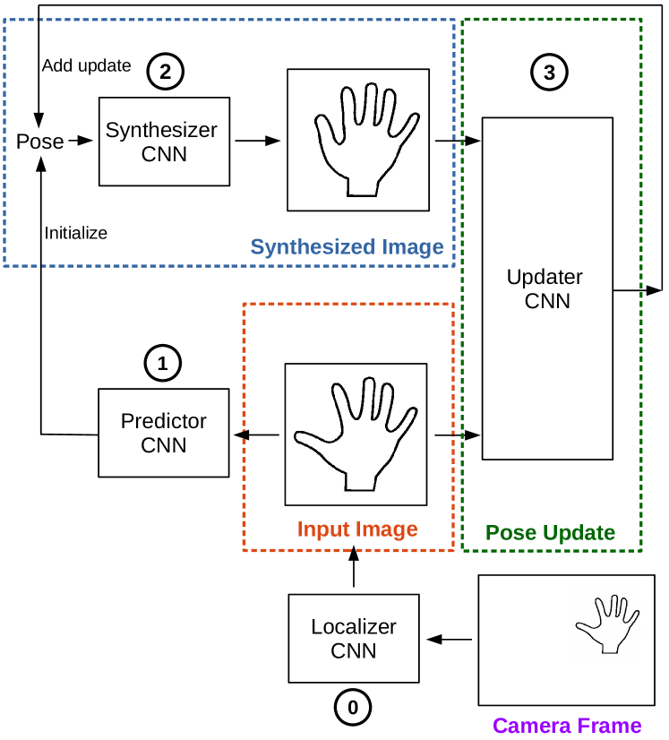
Figure 1: Overview of our approach for hand pose estimation. First, we localize the hand in the camera frame and crop a patch around the hand location. Then, we use a first CNN to predict an initial estimate of the 3D pose given an input depth image of the hand. The pose is used to synthesize a depth image , which is used together with the input depth image to derive a pose update . The update is applied to the pose and the process is iterated. In this work, we follow this general approach and further show how to extend it to joint hand-object pose estimation.

We then introduce a method that learns to provide updates for improving the current estimate of the pose, given the input depth image and the image generated for this pose estimate as shown in Fig. 1. By iterating this method a number of times, we can correct the mistakes of an initial estimate provided by a simple discriminative method. All the components are implemented as Deep Networks with simple architectures.

Not only is it interesting to see that all the components needed for hand registration that used to require careful design can be learned instead, but we will also show that our approach has en-par performance compared to the state-of-the-art methods. It is also very efficient and runs in real-time on a single GPU.

This method was originally published in [29]. Here, we also show how to generalize our feedback loop to the challenging task of jointly estimating the 3D poses of a hand and an object, while the hand interacts with the object. This is inherently challenging, since the object introduce additional occlusions, and enlarge the joint configuration space. In such a case, we first estimate an initial poses for the hand and the object separately, and then fuse these initial predictions within our feedback framework to increase accuracy of the two poses. For this complex problem, our novel approach works on each frame independently, and does not require a good initialization as current tracking-based approaches do [30, 31], while still outperforming the state-of-the-art when using depth images only.

Our approach is related to generative approaches [32], in particular [33] which also features a feedback loop reminiscent of ours. However, our approach is deterministic and does not require an optimization based on distribution sampling, on which generative approaches generally rely, but which tends to be inefficient.

In the remainder of the paper, we first give a short review of related work in Section 2. We describe our approach for hands in isolation in Section 3, introduce the extension for hands and objects in Section 4. Finally, we evaluate our method for hand pose estimation in Section 5 and for joint hand-object pose estimation in Section 6.

2 Related Work

Hand pose estimation is a frequently visited problem in Computer Vision, and is the subject of a plethora of published work. We refer to [1] for an overview of earlier work, and here we will discuss only more recent work, which can be divided into two types of approaches.

2.1 Discriminative Methods

The first type of approaches is based on discriminative models that aim at directly predicting the joint locations from RGB or RGB-D images. Some recent works, including [2, 3, 34, 7, 8] use different approaches with Random Forests, but are restricted to static gestures, showing difficulties with occluded joints, or causing high inaccuracies at finger tips. These problems have been addressed by more recent works [35, 16, 36, 11, 37, 10, 12, 13, 14, 15] that use Convolutional Neural Networks, nevertheless they are still not as accurate as generative methods that we discuss next.

2.2 Generative Methods

Our approach is more related to the second type, which covers generative, model-based methods. The works of this type are developed from four generic building blocks: (1) a hand model, (2) a similarity function that measures the fit of the observed image to the model, (3) an optimization algorithm that maximizes the similarity function with respect to the model parameters, and (4) an initial pose from which the optimization starts.

For the hand model, different hand-crafted models were proposed. The choice of a simple model is important for maintaining real-time capabilities, and representing a trade-off between speed and accuracy as a response to a potentially high degree of model abstraction. Different hand-crafted geometrical approximations for hand models were proposed. For example, [6] uses a hand model consisting of spheres, [5] adds cylinders, ellipsoids, and cones. [21] models the hand from a Sum of Gaussians. More holistic hand representations are used by [17, 20, 22], with a linear blend skinning model of the hand that is rendered as depth image. [9] increases the matching quality by using depth images that resemble the same noise pattern as the depth sensor. [18] uses a fully shaded and textured triangle mesh controlled by a skeleton.

Different modalities were proposed for the similarity function, which are coupled to the used model. The modalities include, e.g., depth values [4, 23, 6], salient points, edges, color [18], or combinations of these [17, 5, 21, 22].

The optimization of the similarity function is a critical part, as the high dimensional pose space is prone to local minima. Thus, Particle Swarm Optimization is often used to handle the high dimensionality of the pose vector [23, 5, 6, 20]. Differently, [17, 18, 21] use gradient-based methods to optimize the pose, while [4] uses dynamics simulation. Due to the high computation time of these optimization methods, which have to be solved for every frame, [9] does not optimize the pose but only evaluates the similarity function for several proposals to select the best fit. Recent works aim at handcrafting a differentiable similarity function, which tightly integrates the hand model to achieve accurate and fast results [24, 25].

In order to kick-start optimization, [21] uses a discriminative part-based pose initialization, and [6] uses finger tips only. [9] predicts candidate poses using a Hough Forest. [18] requires predefined hand color and position, and [5] relies on a manual initialization. Furthermore, tracking-based methods use the pose of the last frame [4, 5, 22, 30], which can be problematic if the difference between frames is too large, due to fast motion or low frame rates.

Our approach differs from previous works in the first three building blocks. We do not use a deformable CAD model of the hand. Instead, we learn from registered depth images to generate realistic depth images of hands, similar to work on inverse graphics networks [26, 38], and other recent work on generating images [39, 40]. This approach is very convenient, since deforming correctly and rendering a CAD model of the hand in a realistic manner requires a significant input of engineering work. Most importantly, it does not require additional training data.

In addition, we do not use a hand-crafted similarity function and an optimization algorithm. We learn rather to predict updates that improve the current estimate of the hand pose from training data, given the input depth image and a generated image for this estimate. Again, this approach is very convenient, since it means we do not need to design the similarity function and the optimization algorithm, neither of which is a simple task.

[41] relies on a given black-box image synthesizer to provide synthetic samples on which the regression network can be trained. It then learns a network to substitute the black-box graphics model, which can ultimately be used to update the pose parameters to generate an image that most resembles the input. In contrast, we learn the generator model directly from training data, without the need for a black-box image synthesizer. Moreover, we will show that the optimization is prone to output infeasible poses or get stuck in local minima and therefore introduce a better approach to improve the pose.

[42] uses an auto-encoder to compute an embedding from the 3D hand pose, and feed the embedding vector to an image synthesizer that outputs a depth image of the hand. This setup is used to synthesize additional training data for training a pose predictor, but in their setup they only aim at generating synthesized images as close as possible to the real images to train a discriminative predictor.

2.3 Feedback

Since we learn to generate images of the hand, our approach is also related to generative approaches, in particular [33], which uses a feedback loop with an updater mechanism akin to ours. It predicts updates for the position from which a patch is cropped from an image, such that the patch fits best to the output of a generative model. However, this step does not predict the full set of parameters. The hidden states of the model are found by a costly sampling process.

[43] proposed an approach related to ours, which also relies on iteratively refining the 2D joint locations for human pose estimation. They use an initial estimate of the 2D joint locations to generate a heatmap with the joint locations. These heatmaps are stacked to the input image and an update is predicted, which, however, does not handle occlusions well. This process is then iterated a few times. In contrast to our work, their approach only works for 2D images due to limitations of the feedback. Also, their training strategy is different, and requires a predefined absolute step size and predefined update directions, which can be hard to learn. In contrast, we use latent update directions with a relative step size.

[44] introduced Feedback Networks for general purpose iterative prediction. They formulate the feedback as a recurrent shared operation where a hidden state is passed on to the next iteration. At each iteration, they predict an absolute output and not an update, which is more difficult. Also, their approach does not use any feedback in the input or output space, so their notion of ”feedback” is only an internal structure of the predictor.

Since the introduction of our feedback method [29], it was successfully applied to other fields, such as 3D object pose estimation. [45] predicts updates on 2D object locations. Similarly, [46] uses a CAD rendering of an object together with the input image to predict an update for the rendered CAD pose to better resemble the object pose in the input image.

2.4 Joint Hand-Object Pose Estimation

The approaches for hand pose estimation discussed so far can only handle minor occlusion, and in practice the accuracy decreases with the degree of occlusion. To specifically account for occlusions, different approaches try to learn an invariance by using images of a hand with an interacting object for training [47, 36] to simulate occlusions, by removing the object for estimating the hand pose [48], or by using temporal information to recover from occlusions [49].

Similar to hands in isolation, accurate methods are available for object pose estimation without occlusions [50, 45]. However, for our problem of joint hand-object pose estimation, object pose methods are required that are specifically robust to partial occlusion. Keypoint-based methods [51, 52] perform well with occlusions, but only on textured objects, and [53] requires discriminative color and features. In order to handle clutter and occlusions, local patch-based methods [54, 55], voting-based methods [56], or segmentation-based methods [57] have shown robustness to clutter and occlusions. However, they only consider objects, and it is not clear how to integrate a hand in these methods.

The problem of hand and object pose estimation is much harder than considering hands or objects in isolation. A straightforward approach of combining methods of both sides does not lead to good results, since the physical constraints and visual occlusions between hand and object are not considered. Several works considered tracking of two hands simultaneously, however, they require hands to be well-separated [58, 27], multiple-views [5], work at non-interactive framerates [59], or accurate segmentation [60, 61]. For handling unknown objects, [62, 63] use an ICP-like object tracking that creates a model of the object on the fly. However, once it looses the temporal tracking, it fails completely. [31] uses a model-based approach for tracking hand-hand and hand-object poses. Similarly, [30] performs model-based tracking of hand and object jointly, but requires a model for the hand and the object. Similar tracking-based approaches where proposed by [64], who consider tracking multiple hands and objects jointly at non-interactive framerates, and by [5], who track a single hand interacting with an object but require several cameras for handling the occlusions. These tracking-based approaches require a good initialization for each frame and are inherently prone to drifting over time. In contrast to these hand-object pose estimation methods, our approach only requires a single depth camera, works without initialization, without temporal tracking, and does not drift over time since we process each frame independently.

3 Method

In this section, we will first give an overview of our method. We then describe in detail the different components of our method: A discriminative approach to predict a first pose estimate, a method able to generate realistic depth images of the hand, and a learning-based method to refine the initial pose estimate using the generated depth images.

3.1 Hand Pose Estimation

Our objective is to estimate the pose $\mathbf{p}$ of a hand in the form of the 3D locations of its joints $\mathbf{p}=\{\mathbf{j}_{i}\}^{J}_{i=1}$ with $\mathbf{j}_{i}=(x_{i},y_{i},z_{i})$ from a single depth image $\mathcal{D}$. In practice, $J=14$ for the dataset we use. We assume that a training set $\mathcal{T}=\{(\mathcal{D}_{i},\mathbf{p}_{i})\}^{N}_{i=1}$ of depth images labeled with the corresponding 3D joint locations is available.

As explained in the introduction, we first train a predictor CNN to predict an initial pose estimate $\widehat{\mathbf{p}}^{(0)}$ in a discriminative manner given an input depth image $\mathcal{D}_{\text{input}}$ centered around the hand location:

$$\widehat{\mathbf{p}}^{(0)}=\operatorname{pred}(\mathcal{D}_{\text{input}})\;\;.$$ (1)

We use a Convolutional Neural Network (CNN) to implement the $\operatorname{pred}(.)$ function with a standard architecture. More details will be given in Section 3.3.

In practice, $\widehat{\mathbf{p}}^{(0)}$ is never perfect, and following the motivation provided in the introduction, we introduce a hand model learned from the training data. As shown in Fig. 2, this model can synthesize the depth image corresponding to a given pose $\mathbf{p}$, and we will refer to this model as the synthesizer CNN:

$$\mathcal{D}_{\operatorname{synth}}=\operatorname{synth}(\mathbf{p})\;\;.$$ (2)

We also use a Deep Network to implement the synthesizer.

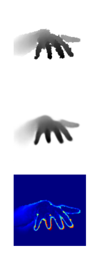
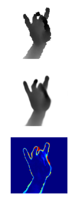
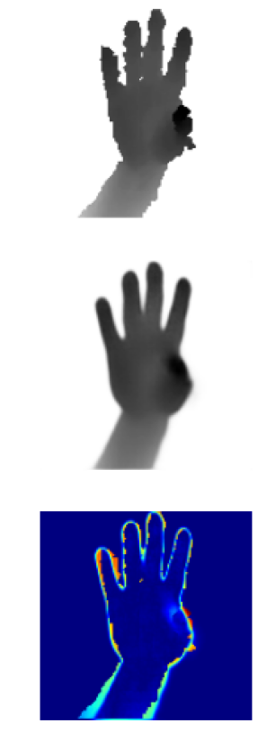
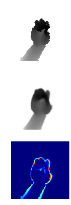
Figure 2: Samples generated by the synthesizer CNN for different poses from the test set. Top: Ground truth depth image. Middle: Synthesized depth image using our learned hand model. Bottom: Color-coded, pixel-wise difference between the depth images. Red represents large errors, blue represents small errors. The synthesizer CNN is able to render convincing depth images for a very large range of poses. The largest errors are located near the occluding contours of the hand, which are noisy in the ground truth images.

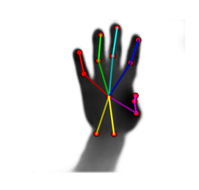
(a)

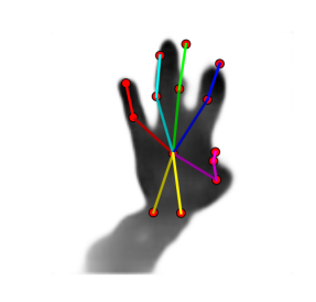
(b)

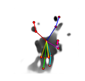
(c)

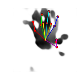
(d)

Figure 3: Synthesized images for physically impossible poses. Note the colors that indicate different fingers. (a) shows a feasible pose with its synthesized image. (b) shows the synthesized image for the same pose after swapping the ring and middle finger positions. In (c) the ring and middle finger are flipped downwards, and in (d) the wrist joints are flipped upwards.

A straightforward way of using this synthesizer would consist in estimating the hand pose $\widehat{\mathbf{p}}$ by minimizing the squared loss between the input image and the synthetic one:

$$\widehat{\mathbf{p}}=\operatorname*{arg\,min}_{\mathbf{p}}\lVert\mathcal{D}_{\text{input}}-\operatorname{synth}(\mathbf{p})\rVert^{2}\;\;.$$ (3)

This is a non-linear least-squares problem, which can potentially be solved iteratively using $\widehat{\mathbf{p}}^{(0)}$ as initial estimate. However, the objective function of Eq. (3) exhibits many local minima. Moreover, during the optimization of Eq. (3), $\mathbf{p}$ can take values that correspond to physically infeasible poses. For such values, the output $\operatorname{synth}(\mathbf{p})$ of the synthesizer CNN is unpredictable as depicted in Fig. 3, and this is likely to make the optimization of Eq. (3) diverge or be stuck in a local minimum, as we will show in the experiments in Section 5.4.

We therefore introduce a third function that we call the $\operatorname{updater}(.,.)$. It learns to predict updates, which are applied to the pose estimate to improve it, given the input image $\mathcal{D}_{\text{input}}$ and the image $\operatorname{synth}(\mathbf{p})$ produced by the synthesizer CNN:

$$\widehat{\mathbf{p}}^{(i+1)}\;\leftarrow\;\widehat{\mathbf{p}}^{(i)}+\operatorname{updater}(\mathcal{D}_{\text{input}},\operatorname{synth}(\widehat{\mathbf{p}}^{(i)}))\;\;.$$ (4)

We iterate this update several times to improve the initial pose estimate. Again, the $\operatorname{updater}(.,.)$ function is implemented as a Deep Network.

We detail below how we implement and train the $\operatorname{pred}(.)$, $\operatorname{synth}(.)$, and $\operatorname{updater}(.,.)$ functions.

3.2 Learning the Localizer Function $\operatorname{loc}(.)$

In practice, we require an input depth image centered on the hand location. In our original paper [29], we relied on a common heuristic that uses the center-of-mass for localizing the hand [35, 7]. In this work, we improve this heuristic by introducing the localizer CNN $\operatorname{loc}(.)$. We still use the center-of-mass for the initial localization from the depth camera frame, but apply an additional refinement step that improves the final accuracy [36, 11]. This refinement step relies on the localizer CNN. The CNN is applied to the 3D bounding box centered on the center-of-mass, and is trained to predict the location of the Metacarpophalangeal (MCP) joint of the middle finger, which we use as referential. The localizer CNN has a simple network architecture, which is shown in Fig. 4.

We train the localizer CNN, parametrized by $\phi$, by optimizing the cost function:

$$\widehat{\phi}=\operatorname*{arg\,min}_{\phi}\sum_{(\mathcal{D},\mathbf{p})\in\mathcal{T}}\lVert\operatorname{loc}_{\phi}(\mathcal{D})-\mathbf{l}\rVert^{2}\;\;.$$ (5)

$\mathbf{l}$ denotes the offset in image coordinates and depth between the center-of-mass and the MCP of the hand. For inference, we crop a depth image from the depth camera frame centered on the center-of-mass, then predict the MCP location by applying $\operatorname{loc}(.)$ to this crop, and finally crop again from the depth camera frame using the predicted location.

We crop the training depth images and the original input depth images around the locations provided by $\operatorname{loc}_{\phi}(.)$ for these images: $\mathcal{D}$ in Eqs. (6), (7), (8), (10), (11), (12) therefore denotes a training depth image after cropping, and $\mathcal{D}_{\text{input}}$ the original input depth image after cropping.

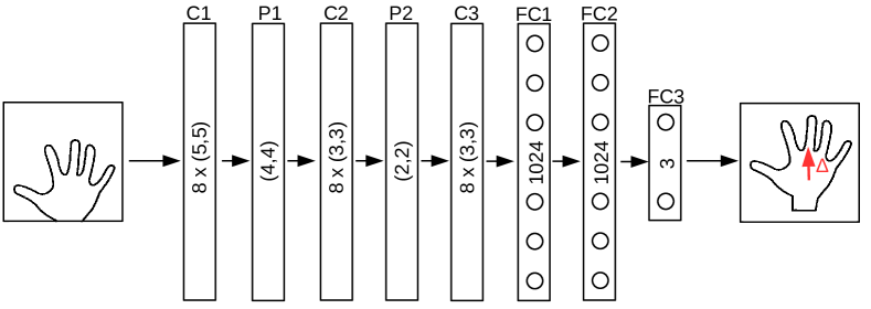
Figure 4: Network architecture of the localizer CNN. All layers have rectified-linear units, except the last layer which has linear units. C denotes a convolutional layer with the number of filters and the filter size inscribed, FC a fully connected layer with the number of neurons, and P a max-pooling layer with the window size. The initial hand crop from the depth image is fed to the network that predicts the location of the MCP of the hand to correct an inaccurate hand localization.

3.3 Learning the Predictor Function $\operatorname{pred}(.)$

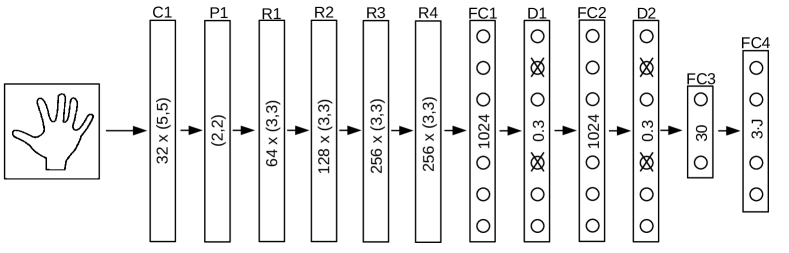
Figure 5: Network architecture of the predictor CNN used for initial pose prediction. C denotes a convolutional layer with the number of filters and the filter size inscribed, FC a fully-connected layer with the number of neurons, D a Dropout layer [65] with the probability of dropping a neuron, R a residual module [66] with the number of filters and filter size, and P a max-pooling layer with the window size. The cropped depth image is fed to the ResNet that predicts the 3D hand pose. The last layer is a bottleneck layer with 30 neurons that incorporates the pose prior. [11]

The predictor CNN $\operatorname{pred}(.)$ is implemented as a neural network. For our experiments with hands in isolation, we use DeepPrior++ [11] as initialization with the architecture shown in Fig. (5). In the spirit of [35, 11], we use a prior on the 3D hand pose, which is integrated into the predictor CNN of the hand. We rely on a simple linear prior $\mathbf{P}(.)$, obtained by a PCA of the 3D hand poses [35]. Thus, $\operatorname{pred}(.)$ predicts the parameters of the pose prior instead of the 3D joint locations, which are obtained by applying the inverse prior to the estimated parameters. The predictor CNN is parametrized by $\Phi$, which is obtained by minimizing

$$\widehat{\Phi}=\operatorname*{arg\,min}_{\Phi}\sum_{(\mathcal{D},\mathbf{p})\in\mathcal{T}}\lVert\mathbf{P}^{-1}(\operatorname{pred}_{\Phi}(\mathcal{D}))-\mathbf{p}\rVert^{2}\;\;.$$ (6)

3.4 Learning the Synthesizer Function $\operatorname{synth}(.)$

We also use a neural network to implement the synthesizer CNN $\operatorname{synth}(.)$, and we train it using the set $\mathcal{T}$ of annotated training pairs. The network architecture is strongly inspired by [26], and is shown in Fig. 6. It consists of four hidden layers, which learn an initial latent representation of feature maps apparent after the fourth fully connected layer FC4. These latent feature maps are followed by several unpooling and convolution layers. The unpooling operation, used for example by [26, 39, 67], is the inverse of the max-pooling operation: The feature map is expanded, in our case by a factor of 2 along each image dimension. The emerging ”holes” are filled with zeros. The expanded feature maps are then convolved with trained 3D filters to generate another set of feature maps. These unpooling and convolution operations are applied subsequently. The last convolution layer combines all feature maps to generate a depth image.

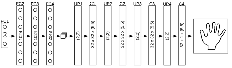
Figure 6: Network architecture of the synthesizer CNN used to generate depth images of hands given their poses. The input of the network is the hand pose. The fully connected hidden layers create a 2048 dimensional latent representation at FC4 which is reshaped into 32 feature maps of size $8\times 8$. The feature maps are gradually enlarged by successive unpooling and convolution operations. The last convolution layer combines the feature maps to derive a single depth image of size $128\times 128$. All layers have rectified-linear units, except the last layer which has tanh units. C denotes a convolutional layer with the number of filters and the filter size inscribed, FC a fully connected layer with the number of neurons, and UP an unpooling layer with the upscaling factor.

We learn the parameters $\widehat{\Theta}$ of the network by minimizing the difference between the generated depth images $\operatorname{synth}(\mathbf{p})$ and the training depth images $\mathcal{D}$ as

$$\widehat{\Theta}=\operatorname*{arg\,min}_{\Theta}\sum_{(\mathcal{D},\mathbf{p})\in\mathcal{T}}\frac{1}{|\mathcal{D}|}\lVert\operatorname{synth}_{\Theta}(\mathbf{p})-\mathcal{D}\rVert^{2}\;\;.$$ (7)

We perform the optimization in a layer-wise fashion. We start by training the feature maps of resolution $8\times 8$. Then we gradually enlarge the output resolution by adding another unpooling and convolutional layer and train again, which achieves lesser errors than end-to-end training in our experience.

The synthesizer CNN is able to generate accurate images, maybe surprisingly well for such a simple architecture. The median pixel error on the test set of the NYU dataset [16] is only 0.1 mm. However, the average pixel error is $8.9$ mm with a standard deviation of $28.5$ mm. This is mostly due to noise in the input images along the outline of the hand, which is smoothed away by the synthesizer CNN. The average depth accuracy of the sensor is $11$ mm [68] in practice.

3.5 Learning the Updater Function $\operatorname{updater}(.,.)$

The updater CNN $\operatorname{updater}(.,.)$ takes two depth images as input. As already stated in Eq. (4), at run-time, the first image is the input depth image, the second image is the image returned by the synthesizer CNN for the current pose estimate. Its output is an update that improves the pose estimate. The architecture is shown in Fig. 7. The input to the network is the observed image stacked channel-wise with the image from the synthesizer CNN. We do not use max-pooling here, but a filter stride [69, 70] to reduce the resolution of the feature maps. We experienced inferior accuracy with max-pooling compared to that with stride, probably because max-pooling introduces spatial invariance [71] that is not desired for this task.

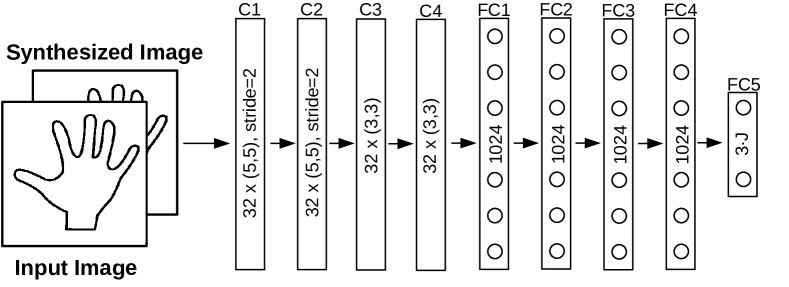
Figure 7: Network architecture of the updater CNN. The network contains several convolutional layers that use a filter stride to reduce the size of the feature maps. The final feature maps are fed into a fully connected network. All layers have rectified-linear units, except the last layer which has linear units. The pose update is used to refine the initial pose and the refined pose is again fed into the synthesizer CNN to iterate the whole procedure. As in Fig. 6, C denotes a convolutional layer, and FC a fully connected layer.

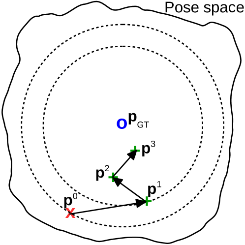
Figure 8: Our iterative pose optimization in high-dimensional space, schematized here in 2D. We start at an initial pose ($\bm{\times}$) and want to converge to the ground truth pose ($\bm{\circ}$), that maximizes image similarity. Our updater CNN generates updates for each pose ($\bm{+}$) that bring us closer. The updates are predicted from the synthesized image of the current pose estimate and the observed depth image.

Ideally, the output of the updater CNN should bring the pose estimate to the correct pose in a single step. This is a very difficult problem, though, and we could not get the network to reduce the initial training error within a reasonable timeframe. However, our only requirement from the updater CNN is for it to output an update which brings us closer to the ground truth as shown in Fig. 8. We iterate this update procedure to get closer step-by-step. Thus, the update should follow the inequality

$$\lVert\mathbf{p}+\operatorname{updater}(\mathcal{D},\operatorname{synth}(\mathbf{p}))-\mathbf{p}_{\text{GT}}\rVert<\lambda\lVert\mathbf{p}-\mathbf{p}_{\text{GT}}\rVert\;\;,$$ (8)

where $\mathbf{p}_{\text{GT}}$ is the ground truth pose for image $\mathcal{D}$, and ${\lambda\in[0,1]}$ is a multiplicative factor that specifies a minimal improvement. We use $\lambda=0.6$ in our experiments.

We optimize the parameters $\Omega$ of the updater CNN by minimizing the following cost function

$$\mathcal{L}=\sum_{(\mathcal{D},\mathbf{p})\in\mathcal{T}}\sum_{\mathbf{p}^{\prime}\in\mathcal{T}_{\mathcal{D}}}\max(0,\lVert\mathbf{p}^{\prime\prime}-\mathbf{p}\rVert-\lambda\lVert\mathbf{p}^{\prime}-\mathbf{p}\rVert)\;\;,$$ (9)

where $\mathbf{p}^{\prime\prime}=\mathbf{p}^{\prime}+\operatorname{updater}_{\Omega}(\mathcal{D},\operatorname{synth}(\mathbf{p}^{\prime}))$, and $\mathcal{T}_{\mathcal{D}}$ is a set of poses. The introduction of the synthesizer CNN allows us to virtually augment the training data and add arbitrary poses to $\mathcal{T}_{\mathcal{D}}$, which the updater CNN is then trained to correct.

The set $\mathcal{T}_{\mathcal{D}}$ contains the ground truth $\mathbf{p}$, for which the updater CNN should output a zero update. We further add as many meaningful deviations from that ground truth as possible, which the updater CNN might perceive during testing and be asked to correct. We start by including the output pose of the predictor CNN $\operatorname{pred}(\mathcal{D})$, which is used during testing as initialization of the update loop. Additionally, we add copies with small Gaussian noise for all poses. This creates convergence basins around the ground truth, in which the predicted updates point towards the ground truth, as we show in the evaluation, and helps to explore the pose space.

After every 2 epochs, we augment the set by applying the current updater CNN to the poses in $\mathcal{T}_{\mathcal{D}}$, that is, we permanently add the set

$$\{\mathbf{p}_{2}\;|\;\exists\mathbf{p}\in\mathcal{T}_{\mathcal{D}}\text{ s.t. }\mathbf{p}_{2}=\mathbf{p}+\operatorname{updater}(\mathcal{D},\operatorname{synth}(\mathbf{p}))\}\;$$ (10)

to $\mathcal{T}_{\mathcal{D}}$. This extends the training set with poses made of the predicted updates from the current training set $\mathcal{T}_{\mathcal{D}}$. This forces the updater CNN to learn to further improve on its own outputs.

In addition, we sample from the current distribution of errors across all the samples, and add these errors to the poses, thus explicitly focusing the training on common deviations. This is different from the Gaussian noise and helps to predict correct updates for larger initialization errors.

3.6 Learning all Functions Jointly

So far, we have considered optimizing all functions separately, i.e., first training the synthesizer CNN and the predictor CNN, and then using them to train the updater CNN. However, it is theoretically possible to train the three networks together. One iteration can be expressed in terms of the current pose $\mathbf{p}$ by introducing the following $\operatorname{iter}(.)$ function:

$$\operatorname{iter}(\mathbf{p})=\mathbf{p}+\operatorname{updater}(\operatorname{synth}(\mathbf{p}),\mathcal{D})\;\;.$$ (11)

The pose estimate $\widehat{\mathbf{p}}^{(n)}$ after $n$ iterations can be written as:

$$\widehat{\mathbf{p}}^{(n)}=\operatorname{iter}(\ldots\operatorname{iter}(\operatorname{pred}(\mathcal{D}))\ldots)\;\;.$$ (12)

$\operatorname{pred}(.)$, $\operatorname{synth}(.)$, and $\operatorname{updater}(.)$ can now be trained by minimizing

$$\{\widehat{\Phi},\widehat{\Theta},\widehat{\Omega}\}=\operatorname*{arg\,min}_{\{\Phi,\Theta,\Omega\}}\sum_{(\mathcal{D},\mathbf{p})\in\mathcal{T}}\lVert\widehat{\mathbf{p}}^{(n)}-\mathbf{p}\rVert^{2}\;\;.$$ (13)

The function $\operatorname{iter}(.)$ can be seen as a Recurrent Neural Network (RNN) that depends on the input depth image $\mathcal{D}$. In comparison to RNNs, our method makes training simpler, intermediary steps easier to understand, and the design of the networks’ architectures easier.

We tried to optimize Eq. (13) starting from a random network initialization, but the optimization did not converge to a satisfying solution. Also, when using the pretrained synthesizer CNN and predictor CNN as initialization, the optimization converges, but this leads to similar accuracy, indicating that end-to-end optimization is possible, but not useful here. Moreover, the intermediate results, i.e., the synthesized depth images, are less interpretable as the hand is barely recognizable. Splitting the optimization problem as we do makes therefore the optimization easier, at no loss of accuracy.

4 Joint Hand-Object Pose Estimation

We now aim at estimating both the pose $\mathbf{p}^{H}$ of a hand and the pose $\mathbf{p}^{O}$ of an object simultaneously while the hand is manipulating the object. We start the pose prediction by first estimating the locations of the hand and the object within the input image. Using the localization, we predict an initial estimate of the pose for the hand and the object separately. In practice, these poses are not very accurate, since hand and object can severely occlude each other. Therefore, we introduce feedback by first synthesizing depth images of the hand and the object, and merge them together. An overview of our method with the different operations and networks is shown in Fig. 9.

We can then predict an update that aims at correcting the object pose and the hand pose. Each step is performed by a CNN. As in the previous section, we denote them localizer CNN $\operatorname{loc}(.)$, predictor CNN $\operatorname{pred}(.)$, synthesizer CNN $\operatorname{synth}(.)$, and updater CNN $\operatorname{updater}(.,.)$. However, this time we use one network for the hand and one for the object and use suffixes ^H and ^O, respectively, to distinguish them. In the following we detail how the individual networks are trained.

Since we now aim at estimating the hand pose and the object pose simultaneously, we require for the training set the hand pose and the object pose for each depth frame $\mathcal{T}=\{(\mathcal{D}_{i},\mathbf{p}^{O}_{i},\mathbf{p}^{H}_{i})\}^{N}_{i=1}$. Acquiring these annotations for real data can be very cumbersome, and therefore we only use synthetically generated training data, as detailed in the next section.

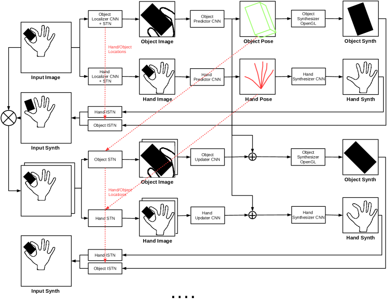
Figure 9: Overview of our joint hand-object pose estimation method. We show the predictors for the initial poses with one iteration of the updaters. The input to our method is a crop from the depth camera frame that contains the hand with the object estimated from the center-of-mass in the depth camera frame. From this input, we localize the hand and the object separately, by predicting the 2D locations and depth using the localizer CNNs. We apply a Spatial Transformer Network (STN) to crop a region of interest around the predicted location. On this centered crop, we predict an initial pose using the predictor CNNs, which are then used to synthesize depth images of the hand and the object using the synthesizer CNNs. Using an Inverse STN (ISTN), we paste back the different inputs, i.e., the synthesized object and the synthesized hand, onto the input image. These images are stacked together ($\otimes$) and serve as input to the updater CNNs that predict one update for the pose of the hand and one for the object. The updates are added to the poses and the procedure is iterated several times.

4.1 Training Data Generation

Capturing real training data of a hand manipulating an object can be very cumbersome, since in our case it requires 3D hand pose and 3D object pose annotations for each frame. This is hindered by severe occlusions, or not always possible at all. Our approach leverages annotations from datasets of hands in isolation, which are much simpler to capture in practice [72, 6, 7], and data from 3D object models, which are available at large scales [73]. We use an OpenGL-based rendering of the 3D object model and fuse the rendering with the frames from a 3D hand dataset. Since we use depth images, we can simply take the minimum of both depth images for each pixel. We render the object on top of the hand, placing the object near the fingers, and apply a simple collision detection, such that the object is not placed “within” the hand point cloud. The object poses, i.e., rotations and translations, are sampled randomly, constrained by the collision detection. In order to account for sensor noise, we add small Gaussian noise to the rendering. In Fig. 10 we show some samples of synthesized training data.

Besides this semi-synthetic training data, we also use completely synthetic training data of hands and objects. We therefore use a marker-based motion capture system [74] to capture the hand and object pose while the hand is manipulating different objects. Since the image data is corrupted with the markers, we render a synthetic hand model and the CAD object model given the captured poses, and use this rendering as additional training data. This dataset comprises five users performing gestures with five different hand-held objects. In total, 73k frames are synthetically rendered from the captured poses from different viewpoints and used for training.

Figure 10: Training samples used for joint hand-object pose estimation. Top row: Semi-synthetic training data comprising real depth images of hands with rendered objects. The interaction between hand and object cannot be accurately modeled easily, but the solution space of possible object locations and possible object poses can be significantly reduced, which enables training our proposed method. Bottom row: Additional synthetic depth data is used to accurately model the hand-object interaction, but it does not capture the sensor characteristics.

4.2 Learning the Hand and Object Localizers

During experiments we have found that accurate localization of the hand and the object is crucial for accurate pose estimation. Since we jointly consider a hand and an object, we use the combined center-of-mass to perform a rough localization and extract a larger cube around the center-of-mass that contains the hand and the object. Then, we use two CNNs to perform the localization of the hand and the object separately. We train two networks, $\operatorname{loc}^{H}(.)$ for the hand, and $\operatorname{loc}^{O}(.)$ for the object, both taking the same input image cropped from the center-of-mass location. The network architectures are the same as the one used in Section 3.2 and shown in Fig. 4. The networks are trained to predict the 2D location and depth of the MCP joint of the hand $\mathbf{l}^{H}$ and the object centroid $\mathbf{l}^{O}$, respectively, relative to the center-of-mass. Formally, we optimize the cost function

$$\widehat{\Gamma}=\operatorname*{arg\,min}_{\Gamma}\sum_{(\mathcal{D},\mathbf{l}^{H})\in\mathcal{T}}\lVert\operatorname{loc}_{\Gamma}^{H}(\mathcal{D})-\mathbf{l}^{H}\rVert^{2}$$ (14)

for the hand localizer, and

$$\widehat{\chi}=\operatorname*{arg\,min}_{\chi}\sum_{(\mathcal{D},\mathbf{l}^{O})\in\mathcal{T}}\lVert\operatorname{loc}_{\chi}^{O}(\mathcal{D})-\mathbf{l}^{O}\rVert^{2}$$ (15)

for the object localizer, where $\Gamma$ and $\chi$ are the parameters of the localizer CNNs.

4.3 Spatial Transformer and Inverse Spatial Transformer Networks

Once we are given the location of the hand and the object, we use them to crop a region of interest around the hand and the object, respectively, using a Spatial Transformer Network (STN). Note that this makes the crop differentiable and thus trainable end-to-end, and allows faster inference on the GPU since we can run a single large network made from the individual CNNs. The STN proposed in [75] was parametrized to work with 2D images. In this work, we apply the STN on 2.5D depth images. We estimate the spatial transformation $A_{\theta}$ from the 3D location, calculated from the predicted 2D location and depth. Using the intrinsic camera calibration we denote the projection from 3D to 2D as $\operatorname{proj}(\cdot)$, the 3D bounding box as $c$, and the 3D location as $\mathbf{t}$. We can estimate the 2D bounding box projection as $(x^{\pm},y^{\pm})=\operatorname{proj}(\mathbf{t}\pm c)$ and define $x^{\Delta}=(x^{+}-x^{-})$ and $y^{\Delta}=(y^{+}-y^{-})$. This leads to the parametrization of the spatial transformation $A_{\theta}$ as:

$$A_{\theta}=\begin{pmatrix}x^{\Delta}/2&0&x^{-}+x^{\Delta}/2\\ 0&y^{\Delta}/2&y^{-}+y^{\Delta}/2\\ 0&0&1\end{pmatrix}\;\;,$$ (16)

for the parametrization of the sampling grid locations as in [75]. The source sampling grid locations $(x^{s},y^{s})$ are obtained by transforming the regularly sampled target grid locations $(x^{t},y^{t})$ as:

$$(x^{s},y^{s})^{T}=A_{\theta}\cdot(x^{t},y^{t},1)^{T}\;\;.$$ (17)

We then use bilinear sampling to interpolate the depth values of input depth image $\mathcal{D}$ of size $W\times H$:

$$\mathrm{STN}(\mathbf{l},\mathcal{D})=\\ \sum^{H}_{h}\sum^{W}_{w}\mathcal{D}[h,w]\max(0,1-|x^{s}-w|)\max(0,1-|y^{s}-h|)\;\;.$$ (18)

Since we apply a detection and crop using the STN, we require the inverse operation for putting the synthesized object back into the original image frame before applying the updater CNN. Hence, we apply an Inverse STN (ISTN) [76]. It operates the same way as the STN, but uses the inverse of the spatial transformation $A_{\theta}$.

4.4 Learning the Hand and Object Pose Predictors

Once we are given an accurate location of the hand and the object, we crop a patch around the hand and the object using the STN and use the crop to estimate the pose. We denote $c^{H}$ the crop of the hand, and $c^{O}$ the crop of the object. We denote this operation as $c^{O}=\mathrm{STN}(\operatorname{loc}^{O}(\mathcal{D}),\mathcal{D})$. For the pose prediction, we require appropriate parametrization of the hand and object poses. For the object pose $\mathbf{p}^{O}$, we use the eight corners of its 3D bounding box, which was shown to perform better than rotation and translation [77]. For the hand pose, we use the 3D joint locations with a prior, as in Section 3.3, on the 3D hand poses obtained from the data described in Section 4.1. A prior on the 3D hand pose is very effective in case of occlusions, since it constraints the predicted hand pose to valid poses. For our experiments with hands manipulating objects we use a similar architecture to the network shown in Fig. 4 for the sake of speed. However, for the hand predictor CNN $\operatorname{pred}^{H}(.)$ we use $3\cdot J$ neurons for the output layer and for the object predictor CNN $\operatorname{pred}^{O}(.)$ we use $3\cdot 8$ neurons.
Again, we optimize two cost functions to train the predictor CNNs. For the hand pose predictor we optimize

$$\widehat{\eta}=\operatorname*{arg\,min}_{\eta}\sum_{(\mathcal{D},\mathbf{p}^{H})\in\mathcal{T}}\lVert\mathbf{P}^{-1}(\operatorname{pred}_{\eta}^{H}(c^{H}))-\mathbf{p}^{H}\rVert^{2}\;\;,$$ (19)

where $\mathbf{P}$ is the linear prior on the 3D hand poses. For the object pose predictor we optimize

$$\widehat{\Pi}=\operatorname*{arg\,min}_{\Pi}\sum_{(\mathcal{D},\mathbf{p}^{O})\in\mathcal{T}}\lVert\operatorname{pred}_{\Pi}^{O}(c^{O})-\pi(\mathbf{p}^{O})\rVert^{2}\;\;,$$ (20)

where $\pi(\cdot)$ returns the 3D bounding box coordinates given the object pose. $\eta$ and $\Pi$ denote the parameters of the predictor CNNs. We use orthogonal Procrustes analysis [78] to obtain the 3D object pose from the output of $\operatorname{pred}^{O}(.)$.

4.5 Learning the Hand and Object Updaters

Since we now have initial estimates of the pose for the hand and the object, we can use them to start a feedback loop that considers the interaction of hand and object. Therefore, we extend the input data of the updater CNN with the synthesized image of the hand and the object given the initially predicted poses. This requires training a synthesizer CNN, or using a software renderer. Since we have the 3D model of the object readily available, we implement the object synthesizer $\operatorname{synth}^{O}(.)$ with an OpenGL-based renderer. During our experiments, we also evaluated training the updater CNN with the object synthesizer CNN, and this resulted in similar results compared to the OpenGL-based rendering. The hand synthesizer CNN $\operatorname{synth}^{H}(.)$ is trained in the same way as described in Section 3.4. Also, the network architecture of the updater CNN is the same as shown in Fig. 7 in the previous section.

For training the updater CNN, the synthesized images are merged into a single depth image:

$$\begin{split}S=\min(&\mathrm{ISTN}(\operatorname{loc}^{H}(\mathcal{D}),\operatorname{synth}(\mathbf{p}^{H})),\\ &\mathrm{ISTN}(\operatorname{loc}^{O}(\mathcal{D}),\operatorname{synth}(\mathbf{p}^{O})))\otimes\mathcal{D}\;\;,\end{split}$$ (21)

where $\min(A,B)$ denotes the pixel-wise minimum between two depth images $A$ and $B$, and $\otimes$ denotes a channel-wise stacking. We then train the updater CNN for the hand $\operatorname{updater}^{H}(.,.)$ and the object $\operatorname{updater}^{O}(.,.)$ by minimizing the following cost function:

$$\sum_{(\mathcal{D},\mathbf{p}^{H},\mathbf{p}^{O})\in\mathcal{T}}\sum_{\mathbf{p}^{\prime O}\in\mathcal{T}_{O}}\sum_{\mathbf{p}^{\prime H}\in\mathcal{T}_{H}}\max(0,\lVert\mathbf{p}^{\prime\prime}-\mathbf{p}\rVert-\lambda\lVert\mathbf{p}^{\prime H,O}-\mathbf{p}\rVert)\;\;,$$ (22)

where $\mathbf{p}^{\prime\prime}=\mathbf{p}^{\prime H,O}+\operatorname{updater}^{H,O}(c^{H,O},S)$, and $\mathcal{T}_{H}$ and $\mathcal{T}_{O}$ are sets of poses for the hand and the object, respectively. When optimizing Eq. (22) for the hand updater $\operatorname{updater}^{H}(.,.)$, the variables with suffix ^H are used, and when optimizing for the object updater $\operatorname{updater}^{O}(.,.)$ the variables with suffix ^O are used.
When training the updater CNN $\operatorname{updater}^{H}(.,.)$ for the hand, $\mathcal{T}_{H}$ is initialized and updated during training as described in Section 3.5. $\mathcal{T}_{O}$ is made from random poses around the ground truth object pose, and poses from the predictor $\operatorname{pred}^{O}(.)$ applied to training images.
When training the updater CNN $\operatorname{updater}^{O}(.,.)$ for the object, $\mathcal{T}_{O}$ is defined as in Section 3.5. $\mathcal{T}_{H}$ is made from random poses around the ground truth together with predictions from the training data.

For inference, we iterate the updater CNNs several times: We first obtain the initial estimates $\mathbf{p}^{(0)}$ for hand $H$ and object $O$, by running the predictor CNNs on the cropped locations from the localizer CNNs. Then we predict the updates using the merged image $S^{(i)}$ from the previous iteration. Alg. 1 gives a formal expression of this algorithm.

Algorithm 1 Feedback Loop

1:$\widehat{\mathbf{p}}^{(0),H}\leftarrow\operatorname{pred}^{H}(\mathrm{STN}(\operatorname{loc}^{H}(\mathcal{D}),\mathcal{D})$

2:$\widehat{\mathbf{p}}^{(0),O}\leftarrow\operatorname{pred}^{O}(\mathrm{STN}(\operatorname{loc}^{O}(\mathcal{D}),\mathcal{D})$

3:for $i\leftarrow 0$ to $N-1$ do

4:     $\begin{aligned} S^{(i)}\leftarrow\min(&\mathrm{ISTN}(\operatorname{loc}^{H}(\mathcal{D}),\operatorname{synth}(\widehat{\mathbf{p}}^{(i),H})),\\ &\mathrm{ISTN}(\operatorname{loc}^{O}(\mathcal{D}),\operatorname{synth}(\widehat{\mathbf{p}}^{(i),O})))\otimes\mathcal{D}\end{aligned}$

5:     $\widehat{\mathbf{p}}^{(i+1),H}\leftarrow\widehat{\mathbf{p}}^{(i),H}+\operatorname{updater}^{H}(\mathrm{STN}(\mathbf{p}^{(i),H},\mathcal{D}),S^{(i)})$

6:     $\widehat{\mathbf{p}}^{(i+1),O}\leftarrow\widehat{\mathbf{p}}^{(i),O}+\operatorname{updater}^{O}(\mathrm{STN}(\mathbf{p}^{(i),O},\mathcal{D}),S^{(i)})$

7:end for

5 Hand Pose Evaluation

In this section we evaluate our proposed method on the NYU Hand Pose Dataset [16], a challenging real-world benchmark for hand pose estimation. First, we describe how we train the networks. Then, we introduce the benchmark dataset. Furthermore, we evaluate our method qualitatively and quantitatively.

5.1 Training

We optimize the network parameters using gradient descent, specifically using the ADAM method [79] with default hyper-parameters. The batch size is $64$. The learning rate decays over the epochs and starts with $0.001$. The networks are trained for $100$ epochs. We augment the training data online during training by random scales, random crops, and random rotation [11].

We extract a fixed-size metric cube from the depth image around the hand location. The depth values within the cube are resized to a $128\times 128$ patch and normalized to $[-1,1]$. The depth values are clipped to the cube sides front and rear. Points for which the depth is undefined—which may happen with structured light sensors for example—are assigned to the rear side. This preprocessing step was also done in [7] and provides invariance to different hand-to-camera distances.

5.2 Benchmark Dataset

We evaluated our method on the NYU Hand Pose Dataset [16]. This dataset is publicly available and it is backed up by a huge quantity of annotated samples together with very accurate annotations. It also shows a high variability of poses, however, which can make pose estimation challenging. While the ground truth contains $J=36$ annotated joints, we follow the evaluation protocol of [35, 16] and use the same subset of $J=14$ joints.

The training set contains samples of one person, while the test set has samples from two persons. The dataset was captured using a structured light RGB-D sensor, the Primesense Carmine 1.09, and contains over 72k training and 8k test frames. We used only the depth images for our experiments. They exhibit typical artifacts of structured light sensors: The outlines are noisy and there are missing depth values along occluding boundaries.

5.3 Comparison with Baseline

We show the benefit of using our proposed feedback loop to increase the accuracy of the 3D joint localization. For this, we compare our method to very recent state-of-the-art methods: DeepPrior++ [11] integrates a prior on the 3D hand poses into a Deep Network; REN [13] relies on an ensemble of Deep Networks, each operating on a region of the input image; Lie-X [10] uses a sophisticated tracking algorithm constrained to the Lie group; Crossing Nets [42] uses an adversarial training architecture; Neverova et al. [12] proposed a semi-supervised approach that incorporates a semantic segmentation of the hand; DeepModel [15] integrates a 3D hand model into a Deep Network; DISCO [80] learns the posterior distribution of hand poses; Hand3D [14] uses a volumetric CNN to process a point cloud, similar to 3DCNN [81].

We show quantitative comparisons in Table I, which compares the different methods we consider using the average Euclidean distance between ground truth and predicted joint 3D locations, which is a de facto standard for this problem. For our feedback loop, we use DeepPrior++ [11] for initialization as described in Section 3.3, which performs already very accurately. Still, our feedback loop can reduce the error from 12.2 mm to 10.8 mm.

TABLE I: Quantitative evaluation on the NYU dataset [16]. We compare the average Euclidean 3D error of the predicted poses with state-of-the-art methods on the NYU dataset.

Method		Average 3D error
Neverova et al. [12]		14.9mm
Crossing Nets [42]		15.5mm
Lie-X [10]		14.5mm
REN [13]		13.4mm
DeepPrior++ [11]		12.3mm
Feedback [29]		16.2mm
Hand3D [14]		17.6mm
DISCO [80]		20.7mm
DeepModel [15]		16.9mm
Pose-REN [82]		11.8mm
3DCNN [81]		10.6mm
Ours		10.8mm

5.4 Image-Based Hand Pose Optimization

We mentioned in Section 3.1 that the attempt may be made to estimate the pose by directly optimizing the squared loss between the input image and the synthetic one as given in Eq. (3) and we argued that this does not in fact work well. We now demonstrate this empirically.

We used the powerful L-BFGS-B algorithm [83], which is a box constrained optimizer, to solve Eq. (3). We set the constraints on the pose in such a manner that each joint coordinate stays inside the hand cube.

The minimizer of Eq. (3), however, does not correspond to a better pose in general, as shown in Fig. 11. Although the generated image looks very similar to the input image, the pose does not improve, moreover it even often becomes worse. Several reasons can account for this. The depth input image typically exhibits noise along the contours, as in the example of Fig. 11. After several iterations of L-BFGS-B, the optimization may start corrupting the pose estimate with the result that the synthesizer generates artifacts that fit the noise. We quantitatively evaluated the image-based optimization and it gives an average Euclidean error of 32.3 mm on the NYU dataset, which is actually worse than the initial pose of the predictor CNN, which achieves 12.2 mm error.

Furthermore the optimization is prone to local minima due to a noisy error surface [6]. However, we also tried Particle Swarm Optimization [23, 6, 20] a genetic algorithm popular for hand pose optimization, and obtained similar results. This tends to confirm that the bad performance comes from the objective function of Eq. (3) rather than the optimization algorithm.

We further show the histogram of average 3D errors before and after applying the predicted updates for different initializations around the ground truth location in Fig. 13. As evident from the distribution of errors, the updater improves all initializations.

Init	Init	Iter 1	Iter 2	Final

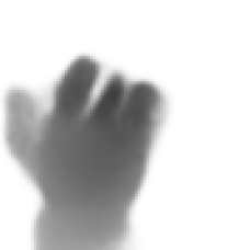
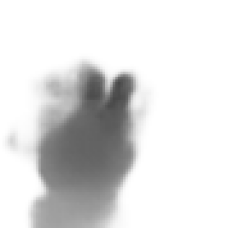
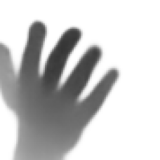
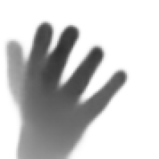
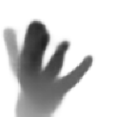
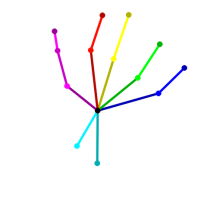
Figure 11: Comparison with image-based pose optimization. (Top) results for image-based optimization, and (bottom) for our proposed method. From left to right: input depth image with initial pose, synthesized image for initial pose, after first, second iteration, and final pose. Minimizing the difference between the synthesized and the input image does not induce better poses due to sensor noise and local minima. Thanks to the updater, our method can fit a good estimate.

5.5 Qualitative results

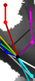
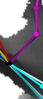
Figure 12: Qualitative results for NYU dataset. We show the inferred joint locations in color and the ground truth in grayscale projected to the depth images. The individual fingers are color coded, where the bones of each finger share the same color, but with a different hue. The left image of each pair shows the initialization and the right image shows the pose after applying our method. Our method applies to a wide variety of poses and is tolerant to noise, occlusions and missing depth values as shown in several images. The rightmost images show a failure case, where the error of the initialization is too large to recover the correct pose and the update only pushes the erroneous joints towards the hand silhouette.

Fig. 12 shows some qualitative examples. For some examples, the predictor provides already a good pose, which we can still improve, especially for the thumb. For worse initializations, also larger updates on the pose can be achieved by our proposed method, to better explain the evidence in the image.

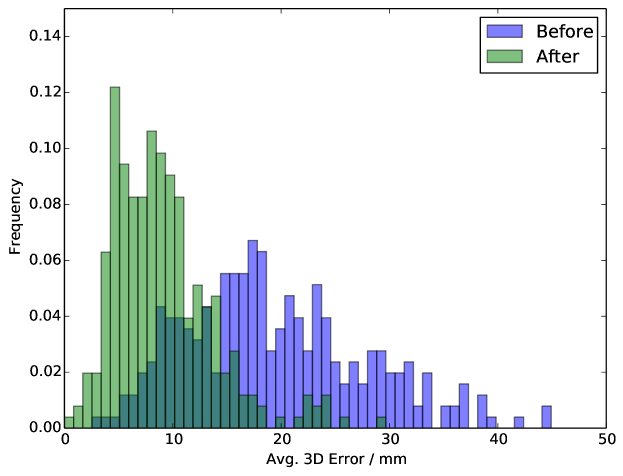
Figure 13: Histogram of errors before and after applying the predicted updates. We initialize noisy joint locations around the ground truth location and calculate the average 3D error before and after applying the update. The different updates minimize the error and thus bring us closer to the ground truth pose.

6 Joint Hand-Object Pose Evaluation

In this section we present the evaluation of our approach for joint hand-object pose estimation on the challenging DexterHO dataset [30]. First, we describe the data we use for training. Then, we introduce the benchmark dataset. Furthermore we evaluate our method qualitatively and quantitatively.

6.1 Training Datasets

Since there are no datasets for joint hand-object pose estimation available that contain enough samples to train a Neural Network, our approach relies on fusing real and synthetic data. We use real hand data and synthetic object data as described in Section 4.1. We use real hand data from the large MSRA [72] dataset, consisting of 76.5k depth frames of hands of 9 different subjects and a wide variety of hand poses. Further, we use the dataset of Qian et al. [6], which contains 2k depth frames of 6 different subjects. Both datasets were captured using a Creative RealSenz Time-of-Flight camera, which is the same camera as used for the experiments on the benchmark dataset. The depth image resolution is $320\times 240$px and the annotations contain $J=21$ joint locations. The 3D object models are manually created from simple geometric primitives to resemble the objects from the benchmark dataset.

6.2 Benchmark Dataset

We evaluated our method on the DexterHO dataset [30] for the task of joint hand-object pose estimation. The dataset contains several sequences of RGB-D data, totaling over 2k frames. There are two different objects used, a large and a small cuboid. The dataset has annotations for both the hand and the object available. The hand annotation contains the 3D location of visible fingertips, and the object annotation consists of three 3D points on the object corners. Although the dataset contains color and depth, we only use the depth images for the evaluation. During our experiments, we noticed some erroneous annotation that we fixed. We will make these corrected annotations available.

6.3 Comparison with Baseline

We evaluate the approach using the metric proposed by [30], which combines the evaluation of the hand and the object poses:

$$E=\frac{1}{|V|+1_{M}}\left[\sum_{i\in V}\lVert X_{i}-G_{i}\rVert+\frac{1_{M}}{3}\sum_{m\in M}\lVert Y_{m}-F_{m}\rVert\right]$$ (23)

The first sum measures the Euclidean distance between the predicted finger tips $X$ and the ground truth finger tips $G$ for all visible finger tips $V$. The second sum measures the Euclidean distance between the predicted object corners $Y$ and the ground truth corners $F$, where $M$ is the set of visible corners. Thereby the object pose is only evaluated if all corners of the object are visible, i.e., the indicator function $1_{M}=3$ if all three corners are visible. Although we predict the 3D location of all joints of the hand, we only use the 3D locations of the finger tips for calculating the error metric. Also, we predict the full 6DoF pose of the object, and calculate the 3D corner locations for the evaluation.

We compare our results to the state-of-the-art on the DexterHO dataset [30] in Table II. Note that the baseline of [30] uses a tracking-based approach, which does not rely on training data but requires the pose of the previous frame as initialization. By contrast, we do not require any initialization at all and predict the poses from scratch on each frame independently. We outperform this strong baseline on two sequences (Rigid and Occlusion), and when [30] use only depth, as we do, we outperform their method on average over all sequences of the dataset. Our method is significantly more accurate for the object corner metric, since it is much easier to acquire training data for objects, compared to hands. For the accuracy of the hand pose estimation, our approach is mostly restricted by the limited training data.

The updaters perform two iterations for the hand and the object, since the results do not improve much for more iterations. Using the feedback loop improves the accuracy on all sequences by 10% on average compared to our initialization.

Note that the two localizer CNNs take the same input data but predict different coordinates, since one is for the hand, the other one for the object. The average localization error of the hand gets 1 mm worse when trained with spherical objects and tested on the DexterHO objects, i.e., cuboids. The localization error of the object gets 40 mm worse when trained on spherical objects and tested on the DexterHO objects. This indicates that the hand localizer CNN, and similarly the hand pose predictor CNN, can still be used with other objects, but the object localizer CNN needs to be object specific.

We also evaluated an approach based on a single CNN predicting both hand and object 3D poses in order to assess the advantage of having two separate networks. In this case, we center the input of the CNN on the center-of-mass of the hand and the object combined together, as described in Section 4.2, and the CNN outputs the poses of the hand and the object concatenated. Training this network appeared more difficult and results in lower accuracy. The average combined error is 36.6 mm, which is significantly more than our proposed approach using a separate CNN for the hand and the object, which achieves an error of 17.6 mm.

TABLE II: Quantitative results on the DexterHO dataset [30]. Note that [30] uses color and depth information together with a tracking-based approach, which relies on a strong pose prior from the previous frame. In comparison, we perform hand and object pose estimation for each frame independently. Also, we use depth information only, for which their reported average error is larger than for our approach. Our approach significantly outperforms the baseline for the accuracy of the object pose on average.

Method	Sequence	Rigid	Rotate	Occlusion	Grasp1	Grasp2	Pinch	Average
Sridhar et al. [30] RGB+Depth	Finger tips	14.2 mm	16.3 mm	17.5 mm	18.1 mm	17.5 mm	10.3 mm	15.6 mm
	Object corners	13.5 mm	26.8 mm	11.9 mm	15.3 mm	15.7 mm	13.9 mm	16.2 mm
	Combined	14.1 mm	18.0 mm	16.4 mm	17.6 mm	17.2 mm	10.9 mm	15.7 mm
Sridhar et al. [30] — Depth only	Combined	–	–	–	–	–	–	18.5 mm
This work init — Depth only	Combined	14.1 mm	20.3 mm	18.8 mm	20.8 mm	24.3 mm	17.6 mm	19.3 mm
Single network — Depth only	Combined	29.0 mm	35.5 mm	35.8 mm	40.1 mm	39.7 mm	39.9 mm	36.6 mm
This work feedback Depth only	Finger tips	14.2 mm	17.9 mm	16.3 mm	22.7 mm	24.0 mm	18.5 mm	18.9 mm
	Object corners	8.4 mm	23.4 mm	7.4 mm	8.2 mm	16.6 mm	9.6 mm	12.4 mm
	Combined	13.2 mm	18.9 mm	14.5 mm	20.2 mm	22.5 mm	16.7 mm	17.6 mm

6.4 Qualitative Results

Fig. 14 shows some qualitative examples on the DexterHO dataset [30], and Fig. 15 shows qualitative results for a sequence where a hand is manipulating a toy duck. Our approach estimates accurate 3D poses for the hand and the object.
Fig. 16 shows the pose for consecutive iterations. The predictor provides an initial estimate of the pose of the hand and the object, and our feedback loop improves these initial poses iteratively.

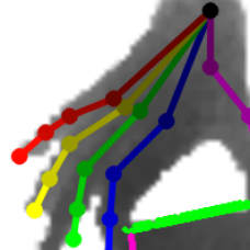
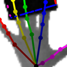
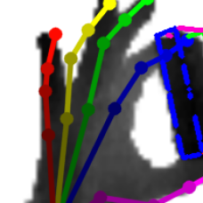
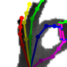
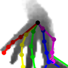
Figure 14: Qualitative results on the DexterHO dataset [30]. Our method provides accurate hand and object pose.

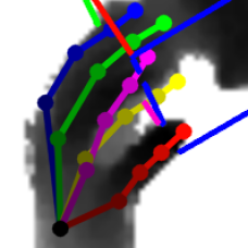
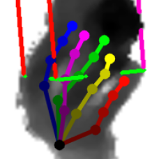
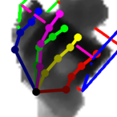
Figure 15: Qualitative results for a hand interacting with a toy duck. Our method provides accurate hand and object poses, also when the hand is manipulating an object.

Initialization
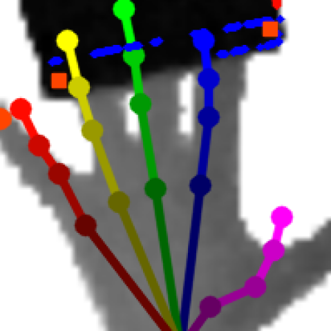
Iteration 1
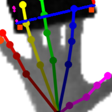
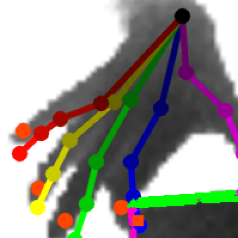
Iteration 2

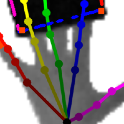
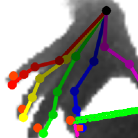
Figure 16: Different iterations on the DexterHO dataset [30]. Top row shows the initialization, and further rows the consecutive iterations. Our results are shown in color, and the ground truth annotations are shown in orange. The ground truth contains the finger tips for the hand, and the corners for the object.

6.5 Runtime

Our method is implemented in Python using the Theano library [84] and we run the experiments on a computer equipped with an Intel Core i7, 64GB of RAM, and an nVidia GeForce GTX 980 Ti GPU. Training takes about ten hours for each CNN. The runtime is composed of the localizer CNN that takes 0.8 ms, the predictor CNN takes 20 ms, the updater CNN takes 1.2 ms for each iteration, and that already includes the synthesizer CNN with 0.8 ms. In practice we iterate our updater CNN twice, thus our method runs at over 40 fps on a single GPU. For the joint hand-object pose estimation we have to run each network once for the hand and once for the object. We run the inference in two threads in parallel, one for the hand and one for the object, and use the predictor CNN with the simpler network architecture that takes 0.8 ms. Thus our approach runs at over 40 fps on a single GPU.

7 Conclusion and Future Work

In this work we presented a novel approach for joint hand-object pose estimation. First, we separate the problem into hand pose and object pose estimation, in order to obtain an initial pose for the hand and the object independently. Then, we introduce a feedback loop, that refines these initial estimates. Remarkably, our approach does not require real data of hand-object interaction and can be trained on synthetic data, which simplifies the creation of the dataset. We evaluated our approach on public datasets. When considering hands only, our approach performs en-par with state-of-the-art approaches. For joint hand-object pose estimation our approach outperforms the state-of-the-art tracking-based approach when using only depth images. Compared to such tracking-based approaches, our approach processes each frame independently, which is important for robustness to drift [20, 85].

It should be noted that our predictor and our synthesizer are trained with exactly the same data. One may then ask how our approach can improve the first estimate made by the predictor. The combination of the synthesizer and the updater network provides us with the possibility for simply yet considerably augmenting the training data to learn the update of the pose: For a given input image, we can draw arbitrary numbers of samples of poses through which the updater is then trained to move closer to the ground truth. In this way, we can explore regions of the pose space which are not present in the training data, but might be returned by the predictor when applied to unseen images.

This work can be extended in several ways. Given the recent trend in 3D hand pose estimation [37, 86, 87], it would be interesting to adapt the feedback loop to color images, which means that the approach also needs to consider lighting and texture. Further, considering a generalization to an object class or different hand shapes would be interesting and could be achieved by adding a shape parameter to the synthesizer CNN. It would also be interesting to see how this approach works with a 3D hand CAD model instead of the synthesizer CNN. Future work could also consider the objective criterion of the updater training such that it would not require the hyperparameters for adding poses.

Markus Oberweger received his MSc Degree in Telematics in 2014 and his PhD Degree in Computer Science in 2018, both from Graz University of Technology. He is currently a Research and Teaching Associate at the Institute for Computer Graphics and Vision at Graz University of Technology. His research interests include Machine Learning methods for Computer Vision, Deep Learning, and methods for 3D pose estimation.

Paul Wohlhart received his MSc Degree in Telematics in 2009 and his PhD Degree in 2014, both from the Graz University of Technology. During his PhD he was working on Machine Learning algorithms and Object Detection and Recognition. He then worked as a Post-doc at the Institute for Computer Graphics and Vision with Prof. Lepetit. He now works as a research engineer at X, the moonshot factory. His research interests include Artificial Intelligence, Computer Vision, and Robotics.

Vincent Lepetit is a Full Professor at the LaBRI, University of Bordeaux, and a senior member of the Institut Universitaire de France (2018-2025). He also supervises a research group in Computer Vision for Augmented Reality at the Institute for Computer Graphics and Vision, TU Graz. His research interests include vision-based Augmented Reality, 3D camera tracking, Machine Learning, object recognition, and 3D reconstruction. He is an editor for the IEEE Transactions on Pattern Analysis and Machine Intelligence, the International Journal of Computer Vision, and the Computer Vision and Image Understanding journal.

References

- [1] A. Erol, G. Bebis, M. Nicolescu, R. D. Boyle, and X. Twombly, “Vision-Based Hand Pose Estimation: A Review,” CVIU, vol. 108, no. 1-2, 2007.
- [2] C. Keskin, F. Kıraç, Y. E. Kara, and L. Akarun, “Real Time Hand Pose Estimation Using Depth Sensors,” in ICCV, 2011.
- [3] ——, “Hand Pose Estimation and Hand Shape Classification Using Multi-Layered Randomized Decision Forests,” in ECCV, 2012.
- [4] S. Melax, L. Keselman, and S. Orsten, “Dynamics Based 3D Skeletal Hand Tracking,” in Proc. of Graphics Interface Conference, 2013.
- [5] I. Oikonomidis, N. Kyriazis, and A. A. Argyros, “Full DOF Tracking of a Hand Interacting with an Object by Modeling Occlusions and Physical Constraints,” in ICCV, 2011.
- [6] C. Qian, X. Sun, Y. Wei, X. Tang, and J. Sun, “Realtime and Robust Hand Tracking from Depth,” in CVPR, 2014.
- [7] D. Tang, H. J. Chang, A. Tejani, and T.-K. Kim, “Latent Regression Forest: Structured Estimation of 3D Articulated Hand Posture,” in CVPR, 2014.
- [8] D. Tang, T. Yu, and T.-K. Kim, “Real-Time Articulated Hand Pose Estimation Using Semi-Supervised Transductive Regression Forests,” in ICCV, 2013.
- [9] C. Xu and L. Cheng, “Efficient Hand Pose Estimation from a Single Depth Image,” in ICCV, 2013.
- [10] C. Xu, L. N. Govindarajan, Y. Zhang, and L. Cheng, “Lie-X: Depth Image Based Articulated Object Pose Estimation, Tracking, and Action Recognition on Lie Groups,” IJCV, 2016.
- [11] M. Oberweger and V. Lepetit, “DeepPrior++: Improving Fast and Accurate 3D Hand Pose Estimation,” in ICCV Workshops, 2017.
- [12] N. Neverova, C. Wolf, F. Nebout, and G. Taylor, “Hand Pose Estimation through Semi-Supervised and Weakly-Supervised Learning,” CVIU, 2017.
- [13] H. Guo, G. Wang, X. Chen, C. Zhang, F. Qiao, and H. Yang, “Region Ensemble Network: Improving Convolutional Network for Hand Pose Estimation,” in ICIP, 2017.
- [14] X. Deng, S. Yang, Y. Zhang, P. Tan, L. Chang, and H. Wang, “Hand3D: Hand Pose Estimation Using 3D Neural Network,” in ARXIV, 2017.
- [15] X. Zhou, Q. Wan, W. Zhang, X. Xue, and Y. Wei, “Model-Based Deep Hand Pose Estimation,” IJCAI, 2016.
- [16] J. Tompson, M. Stein, Y. LeCun, and K. Perlin, “Real-Time Continuous Pose Recovery of Human Hands Using Convolutional Networks,” TOG, vol. 33, 2014.
- [17] L. Ballan, A. Taneja, J. Gall, L. Van Gool, and M. Pollefeys, “Motion Capture of Hands in Action Using Discriminative Salient Points,” in ECCV, 2012.
- [18] M. de La Gorce, D. J. Fleet, and N. Paragios, “Model-Based 3D Hand Pose Estimation from Monocular Video,” PAMI, vol. 33, no. 9, 2011.
- [19] R. Plänkers and P. Fua, “Articulated Soft Objects for Multi-View Shape and Motion Capture,” PAMI, vol. 25, no. 10, 2003.
- [20] T. Sharp, C. Keskin, D. Robertson, J. Taylor, J. Shotton, D. Kim, C. Rhemann, I. Leichter, A. Vinnikov, Y. Wei, D. Freedman, P. Kohli, E. Krupka, A. Fitzgibbon, and S. Izadi, “Accurate, Robust, and Flexible Real-Time Hand Tracking,” in CHI, 2015.
- [21] S. Sridhar, A. Oulasvirta, and C. Theobalt, “Interactive Markerless Articulated Hand Motion Tracking Using RGB and Depth Data,” in ICCV, 2013.
- [22] D. Tzionas, A. Srikantha, P. Aponte, and J. Gall, “Capturing Hand Motion with an RGB-D Sensor, Fusing a Generative Model with Salient Points,” in GCPR, 2014.
- [23] I. Oikonomidis, N. Kyriazis, and A. A. Argyros, “Efficient Model-Based 3D Tracking of Hand Articulations Using Kinect,” in BMVC, 2011.
- [24] A. Tkach, A. Tagliasacchi, E. Remelli, M. Pauly, and A. Fitzgibbon, “Online Generative Model Personalization for Hand Tracking,” TOG, vol. 36, no. 6, p. 243, 2017.
- [25] J. Taylor, L. Bordeaux, T. Cashman, B. Corish, C. Keskin, T. Sharp, E. Soto, D. Sweeney, J. Valentin, B. Luff, A. Topalian, E. Wood, S. Khamis, P. Kohli, S. Izadi, R. Banks, A. Fitzgibbon, and J. Shotton, “Efficient and Precise Interactive Hand Tracking through Joint, Continuous Optimization of Pose and Correspondences,” TOG, vol. 34, no. 4, p. 143, 2016.
- [26] A. Dosovitskiy, J. T. Springenberg, and T. Brox, “Learning to Generate Chairs with Convolutional Neural Networks,” in CVPR, 2015.
- [27] A. Tagliasacchi, M. Schröder, A. Tkach, S. Bouaziz, M. Botsch, and M. Pauly, “Robust Articulated‐ICP for Real‐time Hand Tracking,” CGF, vol. 34, no. 5, pp. 101–114, 2015.
- [28] S. Sridhar, F. Mueller, A. Oulasvirta, and C. Theobalt, “Fast and robust hand tracking using detection-guided optimization,” in CVPR, 2015.
- [29] M. Oberweger, P. Wohlhart, and V. Lepetit, “Training a Feedback Loop for Hand Pose Estimation,” in ICCV, 2015.
- [30] S. Sridhar, F. Mueller, M. Zollhoefer, D. Casas, A. Oulasvirta, and C. Theobalt, “Real-time Joint Tracking of a Hand Manipulating an Object from RGB-D Input,” in ECCV, 2016.
- [31] D. Tzionas, L. Ballan, A. Srikantha, P. Aponte, M. Pollefeys, and J. Gall, “Capturing Hands in Action using Discriminative Salient Points and Physics Simulation,” in IJCV, 2016.
- [32] C. Bishop, Pattern Recognition and Machine Learning. Springer, 2006.
- [33] Y. Tang, N. Srivastava, and R. Salakhutdinov, “Learning Generative Models with Visual Attention,” in NIPS, 2014.
- [34] A. Kuznetsova, L. Leal-taixe, and B. Rosenhahn, “Real-Time Sign Language Recognition Using a Consumer Depth Camera,” in ICCV, 2013.
- [35] M. Oberweger, P. Wohlhart, and V. Lepetit, “Hands Deep in Deep Learning for Hand Pose Estimation,” in CVWW, 2015.
- [36] F. Müller, D. Mehta, O. Sotnychenko, S. Sridhar, D. Casas, and C. Theobalt, “Real-Time Hand Tracking Under Occlusion From an Egocentric RGB-D Sensor,” in ICCV, 2017.
- [37] C. Zimmermann and T. Brox, “Learning to Estimate 3D Hand Pose from Single RGB Images,” in ICCV, 2017.
- [38] T. D. Kulkarni, W. Whitney, P. Kohli, and J. B. Tenenbaum, “Deep Convolutional Inverse Graphics Network,” in NIPS, 2015.
- [39] I. J. Goodfellow, J. Pouget-Abadie, M. Mirza, B. Xu, D. Warde-Farley, S. Ozair, A. Courville, and Y. Bengio, “Generative Adversarial Nets,” in NIPS, 2014.
- [40] T. D. Kulkarni, I. Yildirim, P. Kohli, W. A. Freiwald, and J. B. Tenenbaum, “Deep Generative Vision as Approximate Bayesian Computation,” in NIPS, 2014.
- [41] V. Nair, J. Susskind, and G. E. Hinton, “Analysis-By-Synthesis by Learning to Invert Generative Black Boxes,” in ICANN, 2008.
- [42] C. Wan, T. Probst, L. Van Gool, and A. Yao, “Crossing Nets: Dual Generative Models with a Shared Latent Space for Hand Pose. Estimation,” in CVPR, 2017.
- [43] J. Carreira, P. Agrawal, K. Fragkiadaki, and J. Malik, “Human pose estimation with iterative error feedback,” in CVPR, 2016.
- [44] A. R. Zamir, T.-L. Wu, L. Sun, W. Shen, J. Malik, and S. Savarese, “Feedback Networks,” in CVPR, 2017.
- [45] M. Rad and V. Lepetit, “BB8: A Scalable, Accurate, Robust to Partial Occlusion Method for Predicting the 3D Poses of Challenging Objects without Using Depth,” in ICCV, 2017.
- [46] Y. Li, G. Wang, X. Ji, Y. Xiang, and D. Fox, “DeepIM: Deep Iterative Matching for 6D Pose Estimation,” in ARXIV, 2018.
- [47] G. Rogez, J. S. Supancic, and D. Ramanan, “Understanding Everyday Hands in Action from RGB-D Images,” in ICCV, 2015.
- [48] J. Romero, H. Kjellström, and D. Kragic, “Hands in action: real-time 3D reconstruction of hands in interaction with objects,” in ICRA, 2010.
- [49] M. Madadi, S. Escalera, A. Carruesco, C. Andujar, X. Baró, and J. Gonzàlez, “Occlusion Aware Hand Pose Recovery from Sequences of Depth Images,” in FGR, 2017.
- [50] P. Wohlhart and V. Lepetit, “Learning Descriptors for Object Recognition and 3D Pose Estimation,” in CVPR, 2015.
- [51] D. G. Lowe, “Distinctive image features from scale-invariant keypoints,” IJCV, 2004.
- [52] D. Wagner, T. Langlotz, and D. Schmalstieg, “Robust and unobtrusive marker tracking on mobile phones,” in ISMAR, 2008.
- [53] A. Crivellaro, M. Rad, Y. Verdie, K. M. Yi, P. Fua, and V. Lepetit, “A Novel Representation of Parts for Accurate 3D Object Detection and Tracking in Monocular Images,” in ICCV, 2015.
- [54] E. Brachmann, A. Krull, F. Michel, S. Gumhold, J. Shotton, and C. Rother, “Learning 6D Object Pose Estimation using 3D Object Coordinates,” in ECCV, 2014.
- [55] A. Krull, E. Brachmann, F. Michel, M. Y. Yang, S. Gumhold, and C. Rother, “Learning Analysis-by-Synthesis for 6D Pose Estimation in RGB-D Images,” in ICCV, 2015.
- [56] B. Drost, M. Ulrich, N. Navab, and S. Ilic, “Model globally, match locally: Efficient and robust 3d object recognition,” in CVPR, 2010.
- [57] S. Gupta, P. Arbelaez, R. Girshick, and J. Malik, “Aligning 3D Models to RGB-D Images of Cluttered Scenes,” in CVPR, 2015.
- [58] R. Y. Wang, S. Paris, and J. Popovic, “6D Hands: Markerless Hand Tracking for Computer Aided Design,” 2011.
- [59] I. Oikonomidis, N. Kyriazis, and A. Argyros, “Tracking the articulated motion of two strongly interacting hands,” in CVPR, 2012.
- [60] H. Hamer, K. Schindler, E. Koller-Meier, and L. Van Gool, “Tracking a Hand Manipulating an Object,” in ICCV, 2009.
- [61] D. Goudie and A. Galata, “3D Hand-Object Pose Estimation from Depth with Convolutional Neural Networks,” in FGR, 2017.
- [62] D. Tzionas and J. Gall, “3D Object Reconstruction from Hand-Object Interactions,” in ICCV, 2015.
- [63] P. Panteleris, N. Kyriazis, and A. A. Argyros, “3D Tracking of Human Hands in Interaction with Unknown Objects,” in BMVC, 2015.
- [64] N. Kyriazis and A. A. Argyros, “Scalable 3D Tracking of Multiple Interacting Objects,” in CVPR, 2014.
- [65] N. Srivastava, G. E. Hinton, A. Krizhevsky, I. Sutskever, and R. Salakhutdinov, “Dropout: A Simple Way to Prevent Neural Networks from Overfitting,” JMLR, vol. 15, no. 1, pp. 1929–1958, 2014.
- [66] K. He, X. Zhang, S. Ren, and J. Sun, “Deep Residual Learning for Image Recognition,” in CVPR, 2016.
- [67] M. D. Zeiler, G. W. Taylor, and R. Fergus, “Adaptive Deconvolutional Networks for Mid and High Level Feature Learning,” in ICCV, 2011.
- [68] K. Khoshelham and S. O. Elberink, “Accuracy and Resolution of Kinect Depth Data for Indoor Mapping Applications,” Sensors, vol. 12, no. 2, pp. 1437–1454, 2012.
- [69] A. Jain, J. Tompson, M. Andriluka, G. W. Taylor, and C. Bregler, “Learning human pose estimation features with convolutional networks,” in ICLR, 2014.
- [70] S. Liu, X. Liang, L. Liu, X. Shen, J. Yang, C. Xu, L. Lin, X. Cao, and S. Yan, “Matching-CNN Meets KNN: Quasi-Parametric Human Parsing,” in CVPR, 2015.
- [71] D. Scherer, A. Müller, and S. Behnke, “Evaluation of Pooling Operations in Convolutional Architectures for Object Recognition,” in ICANN, 2010.
- [72] X. Sun, Y. Wei, S. Liang, X. Tang, and J. Sun, “Cascaded Hand Pose Regression,” in CVPR, 2015.
- [73] A. X. Chang, T. Funkhouser, L. Guibas, P. Hanrahan, Q. Huang, Z. Li, S. Savarese, M. Savva, S. Song, H. Su, J. Xiao, L. Yi, and F. Yu, “ShapeNet: An Information-Rich 3D Model Repository,” Stanford University — Princeton University — Toyota Technological Institute at Chicago, Tech. Rep., 2015.
- [74] S. Han, B. Liu, R. Wang, Y. Ye, C. D. Twigg, and K. Kin, “Online Optical Marker-based Hand Tracking with Deep Labels,” TOG, vol. 37, no. 4, pp. 166:1–166:10, 2018.
- [75] M. Jaderberg, K. Simonyan, A. Zisserman, and K. Kavukcuoglu, “Spatial transformer networks,” in NIPS, 2015.
- [76] C.-H. Lin and S. Lucey, “Inverse compositional spatial transformer networks,” in CVPR, 2017.
- [77] Y. Xiang, T. Schmidt, V. Narayanan, and D. Fox, “PoseCNN: A Convolutional Neural Network for 6D Object Pose Estimation in Cluttered Scenes,” RSS, 2018.
- [78] W. Kabsch, “A solution for the best rotation to relate two sets of vectors,” in Acta Crystallographica, 1976.
- [79] D. Kingma and J. Ba, “Adam: A Method for Stochastic Optimization,” in ICLR, 2015.
- [80] D. Bouchacourt, M. P. Kumar, and S. Nowozin, “DISCO Nets: Dissimilarity Coefficient Networks,” in NIPS, 2016.
- [81] L. Ge, H. Liang, J. Yuan, and D. Thalmann, “Real-time 3D Hand Pose Estimation with 3D Convolutional Neural Networks,” PAMI, 2018.
- [82] X. Chen, G. Wang, H. Guo, and C. Zhang, “Pose Guided Structured Region Ensemble Network for Cascaded Hand Pose Estimation,” ARXIV, 2017.
- [83] R. H. Byrd, P. Lu, J. Nocedal, and C. Zhu, “A limited memory algorithm for bound constrained optimization,” SIAM Journal on Scientific and Statistical Computing, vol. 16, no. 5, 1995.
- [84] J. Bergstra, O. Breuleux, F. Bastien, P. Lamblin, R. Pascanu, G. Desjardins, J. Turian, D. Warde-Farley, and Y. Bengio, “Theano: A CPU and GPU Math Expression Compiler,” in Proc. of SciPy, 2010.
- [85] R. Rosales and S. Sclaroff, “Combining Generative and Discriminative Models in a Framework for Articulated Pose Estimation,” IJCV, vol. 67, no. 3, pp. 251–276, May 2006.
- [86] F. Müller, F. Bernard, O. Sotnychenko, D. Mehta, S. Sridhar, D. Casas, and C. Theobalt, “GANerated Hands for Real-Time 3D Hand Tracking from Monocular RGB,” in CVPR, 2018.
- [87] P. Panteleris, I. Oikonomidis, and A. A. Argyros, “Using a Single RGB Frame for Real Time 3D Hand Pose Estimation in the Wild,” in WACV, 2018.