Nonlinear Uncertainty Control with Iterative Covariance Steering

Abstract

This paper considers the problem of steering the state distribution of a nonlinear stochastic system from an initial Gaussian to a terminal distribution with a specified mean and covariance, subject to probabilistic path constraints. An algorithm is developed to solve this problem by iteratively solving an approximate linearized problem as a convex program. This method, which we call iterative covariance steering (iCS), is numerically demonstrated by controlling a double integrator with quadratic drag force subject to additive Brownian noise while satisfying probabilistic path constraints.

I INTRODUCTION

Guidance and control design has generally followed the standard approach where an open-loop reference optimal control is solved with respect to the nonlinear dynamics and then a feedback controller is subsequently designed with respect to the dynamics linearized about the reference trajectory. Hence, there is an implicit unidirectional dependence of the feedback controller on this reference trajectory, but there is no direct mechanism from which the reference trajectory is affected by the closed-loop system behavior. Intuitively, if we could explicitly couple the design of the reference trajectory with the design of the feedback controller, then since we are optimizing over a larger set we could improve closed-loop system performance. The situation becomes more complex with the introduction of state constraints and uncertainty. If the closed-loop statistics of a system are not considered, then the reference trajectory design must be conservative to satisfy the constraints. For systems that are significantly influenced by uncertain external forces, the conservatism of this approach may lead to greatly increased control cost or even infeasibility.

In this paper we consider the system state to be a random vector which evolves according to a nonlinear stochastic differential equation with additive Brownian noise. By letting the state to be a random vector, the control problem can be formulated as one of simultaneously steering each sample trajectory, and as a consequence, we can analytically study the difference between open and closed-loop control [1]. This machinery will serve as our mechanism to understand the coupling between the reference trajectory and the feedback controller. We assume that the state is normally distributed at the initial time, and we will design a control that steers the mean and the covariance of the initial state distribution to some given terminal values at the final time. This problem is referred to as the nonlinear covariance steering (CS) problem. Since the state is assumed to be normally distributed, and thus unbounded, we must treat state constraints probabilistically. That is, the probability that the constraints are satisfied must be greater than some prespecified value. Since, by construction, these constraints may not be met for every sample path, they are often referred to as chance constraints [2, 3].

The special case of linear time-varying stochastic systems with additive Brownian noise has been extensively studied in the literature. It has been shown that if the system is controllable, then the state covariance is also controllable [1]. That is, for an initial covariance $P_{x_{0}}>0$ at time $t_{0}$, there exist a state feedback gain defined on the interval $[t_{0},t_{f}]$ that steers the covariance to any final value $P_{x_{f}}>0$ for any time $t_{f}>t_{0}$. The solution to the optimal linear CS problem with expected quadratic cost was given by Chen et al. [4, 5, 6], and the solution was found to be closely related to the classical linear quadratic feedback control. The discrete linear CS problem with quadratic cost has also been studied and a similar close connection to linear quadratic control has been shown [7].

It is well known that, for linear systems, and in the absence of any constraints, the mean and the covariance have independent dynamics, and that the mean state is controlled by the mean open-loop control and the covariance is controlled by the state feedback gain. It follows that, without constraints, we can consider the mean steering and the covariance steering as separate problems but that, when there are constraints, the mean and covariance are coupled. In other words, for linear systems, the reference trajectory explicitly depends on the closed-loop behavior of the system when the state or control is constrained. For the discrete-time linear case with convex chance constraints, the chance-constrained CS problem can be cast as a deterministic convex optimization problem [8]. This work was later extended to include non-convex chance constraints using mixed-integer programming [9].

In this paper, we propose an algorithmic approach to solve the nonlinear CS problem by iteratively solving the linear CS problem with respect to the reference trajectory of the previous step. This algorithm, which we will refer to as iterative CS (iCS), is a natural extension of linear CS in the spirit of other well known successive approximation methods such as differential dynamic programming (DDP) [10] and iterative LQG (iLQG) [11], which both compute a feedback control by backwards propagating an approximation of the value function. For iCS, we similarly approximate the nonlinear dynamics about a reference trajectory, but, in contrast, the control updates are found by solving a convex program, which has the benefit of allowing direct consideration of probabilistic constraints at the cost of computation time and restricts the approximation of the dynamics to first order.

To the best of our knowledge, there are currently no known methods to solve the nonlinear CS problem. Furthermore, in contrast to the existing literature on chance constrained linear CS, we begin our analysis with a continuous stochastic system and describe an exact discretization procedure.

I-A Notation and Preliminaries

For a random vector $z$ on a probability space $(\Omega,\mathscr{F},\mathbb{P})$, we denote the expectation of a function $f$ of $z$ as $\mathbb{E}[f(z)]$. The mean value of $z$ is denoted by $\bar{z}:=\mathbb{E}(z)$, and the difference from the mean as $\tilde{z}:=z-\mathbb{E}(z)$. The covariance of $z$ is denoted by $P_{z}:=\mathbb{E}(\tilde{z}\tilde{z}^{\mbox{\tiny\sf T}})$. The complement of an event $A\subseteq\Omega$ is denoted $A^{c}=\Omega\setminus A$, and we use the shorthand $\{\omega\in\Omega:z(\omega)\in B\}=\{z\in B\}$ to denote events. Dependence of a quantity $y$ on time $t$ is denoted by $y_{t}$. For a square matrix $A$, we write $A>0$ $(\geq 0)$ if $A$ is positive (semi-)definite, i.e., $x^{\mbox{\tiny\sf T}}Ax>0$ $(\geq 0)$ for all nonzero real vectors $x$. The set of natural numbers, including zero, is written as $\mathbb{N}_{0}$, and $\mathbb{N}_{+}=\mathbb{N}_{0}\setminus\{0\}$. We will denote by $\mathbb{N}_{0}^{m}$ the set of natural numbers up to, and including, a positive integer $m$ (similarly for $\mathbb{N}_{+}^{m}$).

II PROBLEM FORMULATION

Consider the nonlinear stochastic differential equation

$$\mathrm{d}x_{t}=f(x_{t},u_{t},t)\mathrm{d}t+G_{t}\mathrm{d}w_{t},\quad t\in[t_{0},t_{f}],$$ (1)

where $x_{t}\in\mathbb{R}^{n_{x}}$ is the state, $u_{t}\in\mathbb{R}^{n_{u}}$ is the control input, and $w_{t}$ is an $n_{w}$-dimensional standard Brownian motion. At time $t_{0}$, the state $x_{t_{0}}$ is assumed to be normally distributed with fixed mean and covariance

$$\mathbb{E}(x_{t_{0}})=\bar{x}_{0},\quad\mathbb{E}(\tilde{x}_{t_{0}}\tilde{x}_{t_{0}}^{\mbox{\tiny\sf T}})=P_{x_{0}}.$$ (2)

At each time, the state and control are constrained in probability to given convex sets

$$\mathbb{P}(x_{t}\in\mathcal{X}_{t})\geq 1-p_{x,t},\quad\mathbb{P}(u_{t}\in\mathcal{U}_{t})\geq 1-p_{u,t},$$ (3)

where $0<p_{x,t}<1/2$ and $0<p_{u,t}<1/2$ are prescribed maximum probabilities of failure. The constraints (3) are referred to as chance constraints. We wish to find a control that brings the state $x_{t}$ to a final distribution at time $t_{f}$ with given mean and covariance

$$\mathbb{E}(x_{t_{f}})=\bar{x}_{f},\quad\mathbb{E}(\tilde{x}_{t_{f}}\tilde{x}_{t_{f}}^{\mbox{\tiny\sf T}})=P_{x_{f}},$$ (4)

where $P_{x_{f}}$ is a given positive-definite matrix, while minimizing the cost functional

$$J(u)=\int_{t_{0}}^{t_{f}}\big{[}\ell(\bar{u}_{t},\bar{x}_{t})+\mathbb{E}(\tilde{x}_{t}^{\mbox{\tiny\sf T}}Q_{x,t}\tilde{x}_{t}+\tilde{u}_{t}^{\mbox{\tiny\sf T}}Q_{u,t}\tilde{u}_{t})\big{]}\mathrm{d}t.$$ (5)

Here $Q_{x,t}>0$ and $Q_{u,t}\geq 0$ are weight matrices, and $\ell$ is an integrable function that is convex in $\bar{u}_{t}$ and $\bar{x}_{t}$, and the optimization is performed over the control $u$. In summary, we are interested in solving the following problem.

Problem 1

Nonlinear Covariance Steering. Find a control $u_{t}^{*}$ to minimize the cost (5) subject to the dynamics (1), terminal state constraints (4), and chance constraints (3).

In the remainder of this section, we will develop a linear approximation of (1) in the neighborhood of a given reference. Then, after discretizing the linearized system, we will focus our analysis on the discrete linear system.

II-A Time Normalization and Linearization

We begin by normalizing the time domain $[t_{0},t_{f}]$ to the unit interval using the dilation coefficient [12]

$$\sigma\vcentcolon=t_{f}-t_{0}.$$ (6)

Let $\tau\vcentcolon=(t-t_{0})/\sigma\in[0,1]$ be the normalized time, from which it follows that $\sigma=\mathrm{d}t/\mathrm{d}\tau$. Since the Brownian motion increment $\mathrm{d}w_{t}$ has variance $\mathrm{d}t$, we scale the diffusion term in (1) by $\sqrt{\sigma}$ to obtain $\mathrm{d}w_{\tau}$ with variance $\mathrm{d}\tau$ (i.e., $\mathrm{d}w_{t}$ is identically distributed with $\sqrt{\sigma}\mathrm{d}w_{\tau}$). The time normalized system is then given by

$$\mathrm{d}x_{\tau}=\sigma f(x_{\tau},u_{\tau},\tau)\mathrm{d}\tau+\sqrt{\sigma}G_{\tau}\mathrm{d}w_{\tau},\quad\tau\in[0,1],$$ (7)

and the time normalized cost is given by

$$J(u)=\sigma\int_{0}^{1}\big{[}\ell(\bar{u}_{\tau},\bar{x}_{\tau})+\mathbb{E}(\tilde{x}_{\tau}^{\mbox{\tiny\sf T}}Q_{x,\tau}\tilde{x}_{\tau}+\tilde{u}_{\tau}^{\mbox{\tiny\sf T}}Q_{u,\tau}\tilde{u}_{\tau})\big{]}\mathrm{d}\tau.$$ (8)

Next, we linearize (7) about a given reference trajectory $(\hat{x}^{i}_{\tau},\hat{u}^{i}_{\tau})$, where $i\geq 1$ is an index to count successive linearizations. This procedure results in the linear stochastic system

$$\mathrm{d}x_{\tau}\approx(A^{i}_{\tau}x_{\tau}+B^{i}_{\tau}u_{\tau}+r^{i}_{\tau})\mathrm{d}\tau+\sqrt{\sigma}G_{\tau}\mathrm{d}w_{\tau},$$ (9)

where

$$A^{i}_{\tau}\vcentcolon=\sigma\left.\dfrac{\partial f}{\partial x}\right|_{(\hat{x}^{i}_{\tau},\hat{u}^{i}_{\tau})},\quad B^{i}_{\tau}\vcentcolon=\sigma\left.\dfrac{\partial f}{\partial u}\right|_{(\hat{x}^{i}_{\tau},\hat{u}^{i}_{\tau})},\quad$$ (10)

$$r_{\tau}\vcentcolon=\sigma f(\hat{x}^{i}_{\tau},\hat{u}^{i}_{\tau},\tau)-A^{i}_{\tau}\hat{x}^{i}_{\tau}-B^{i}_{\tau}\hat{u}^{i}_{\tau}.$$ (11)

II-B Discrete Approximation

Let $0=\tau_{0}<\tau_{1}<\dots<\tau_{N}=1$ be a partition of the interval $[0,1]$, where

$$\tau_{k}\vcentcolon=\frac{k}{N},\quad k\in\mathbb{N}_{0}^{N}.$$ (12)

Henceforth, we will write $x_{k}\vcentcolon=x_{\tau_{k}}$ and $u_{k}\vcentcolon=u_{\tau_{k}}$. We use a zero-order-hold (ZOH) discretization of the control given by

$$u_{\tau}=u_{k},\quad\tau\in[\tau_{k},\tau_{k+1}),\quad k\in\mathbb{N}_{0}^{N-1}.$$ (13)

Substituting $u_{k}$ in (9), we obtain the solution [13]

$$x_{k+1}=\Phi^{i}(\tau_{k+1},\tau_{k})x_{k}\\ +\int_{\tau_{k}}^{\tau_{k+1}}\Phi^{i}(\tau_{k+1},\tau)(B^{i}_{\tau}\,u_{k}+r^{i}_{\tau})\mathrm{d}\tau\\ +\sqrt{\sigma}\int_{\tau_{k}}^{\tau_{k+1}}\Phi^{i}(\tau_{k+1},\tau)G_{\tau}\mathrm{d}w_{\tau},\quad k\in\mathbb{N}_{0}^{N-1},$$ (14)

where $\Phi^{i}(\tau,s)$ is the state transition matrix for system (9), which satisfies

$$\dfrac{\partial}{\partial\tau}\Phi^{i}(\tau,s)=A^{i}_{\tau}\Phi^{i}(\tau,s),\quad\Phi^{i}(\tau,\tau)=I.$$ (15)

For $k\in\mathbb{N}_{0}^{N-1}$, we rewrite (14) as

$$x_{k+1}=A^{i}_{k}x_{k}+B^{i}_{k}u_{k}+r^{i}_{k}+\sqrt{\sigma}G^{i}_{k}w_{k},$$ (16)

where $w_{k}\in\mathbb{R}^{n_{x}}$ are independent and identically distributed $\mathcal{N}(0,I)$ and where

$$A^{i}_{k} \vcentcolon=\Phi^{i}(\tau_{k+1},\tau_{k}),$$ (17a)

$$B^{i}_{k} \vcentcolon=\int_{\tau_{k}}^{\tau_{k+1}}\Phi^{i}(\tau_{k+1},\tau)B^{i}_{\tau}\mathrm{d}\tau,$$ (17b)

$$r^{i}_{k} \vcentcolon=\int_{\tau_{k}}^{\tau_{k+1}}\Phi^{i}(\tau_{k+1},\tau)r^{i}_{\tau}\mathrm{d}\tau.$$ (17c)

The stochastic integral in (14) is a zero-mean Gaussian random vector with covariance

$$\Sigma=\int_{\tau_{k}}^{\tau_{k+1}}\Phi^{i}(\tau_{k+1},\tau)G_{\tau}G_{\tau}^{\mbox{\tiny\sf T}}\Phi^{i\mbox{\tiny\sf T}}(\tau_{k+1},\tau)\mathrm{d}\tau,$$ (18)

and therefore the matrix $G^{i}_{k}$ is selected such that $G^{i}_{k}w_{k}\in\mathbb{R}^{n_{x}}$ is distributed $\mathcal{N}(0,\Sigma)$. Since $\Sigma$ may have rank greater than $n_{w}$ (e.g., $\Sigma$ is full rank if $(A^{i}_{\tau},G_{\tau})$ is controllable), the matrix $G^{i}_{k}$ must be $n_{x}\times n_{x}$. Furthermore, since the solution to $G^{i}_{k}G^{i\mbox{\tiny\sf T}}_{k}=\Sigma$ is not unique, there exist a continuum of coefficient matrices $G^{i}_{k}$ such that the resulting state processes are equidistributed.

The discrete formulation (14) is an exact representation of the linear system (9) with ZOH control. However, since the previous integrals may be difficult to compute, the following first-order approximation is commonly used:

$$\begin{aligned} &A^{i}_{k}\vcentcolon=A^{i}_{\tau_{k}}\mathrm{d}\tau+I,&\quad B^{i}_{k}&\vcentcolon=B^{i}_{\tau_{k}}\mathrm{d}\tau,\\ &G^{i}_{k}\vcentcolon=\sqrt{\mathrm{d}\tau}G_{\tau_{k}},&\quad r^{i}_{k}&\vcentcolon=r^{i}_{\tau_{k}}\mathrm{d}\tau.\end{aligned}$$ (19)

We remark that the method of discretization chosen does not affect any of the following discussion.

Following [7, 8, 9], we will rewrite the discrete system (16) as a single linear equation. Define the state transition matrix from step $k_{0}$ to step $k_{1}$ as

$$A^{i}_{k_{1},k_{0}}\vcentcolon=\begin{cases}A^{i}_{k_{1}}A^{i}_{k_{1}-1}\cdots A^{i}_{k_{0}},&k_{1}\geq k_{0},\\ I,&k_{1}<k_{0},\end{cases}$$ (20)

and the corresponding transitions for the control, noise, and affine terms as

$$B^{i}_{k_{1},k_{0}}\vcentcolon=A^{i}_{k_{1},k_{0}+1}B_{k_{0}},\quad G^{i}_{k_{1},k_{0}}\vcentcolon=A^{i}_{k_{1},k_{0}+1}G^{i}_{k_{0}},$$ (21)

$$r^{i}_{k_{1},k_{0}}\vcentcolon=A^{i}_{k_{1},k_{0}+1}r_{k_{0}}.$$ (22)

Define concatenated control and disturbance vectors at step $k$ as

$$U_{k} \vcentcolon=\begin{bmatrix}u_{0}^{\mbox{\tiny\sf T}}&u_{1}^{\mbox{\tiny\sf T}}&\cdots&u_{k}^{\mbox{\tiny\sf T}}\end{bmatrix}^{\mbox{\tiny\sf T}}\in\mathbb{R}^{(k+1)n_{u}},$$ (23)

$$W_{k} \vcentcolon=\begin{bmatrix}w_{0}^{\mbox{\tiny\sf T}}&w_{1}^{\mbox{\tiny\sf T}}&\cdots&w_{k}^{\mbox{\tiny\sf T}}\end{bmatrix}^{\mbox{\tiny\sf T}}\in\mathbb{R}^{(k+1)n_{x}}.$$ (24)

Then the state at step $k$ can be written as

$$x_{k}=\bar{A}^{i}_{k}x_{0}+\bar{B}^{i}_{k}U_{k-1}+\bar{r}^{i}_{k}1_{k}+\sqrt{\sigma}\bar{G}^{i}_{k}W_{k-1},$$ (25)

where $1_{k}\in\mathbb{R}^{k}$ is a column vector of ones, $\bar{A}^{i}_{k}\vcentcolon=A^{i}_{k-1,0}$, and

$$\bar{B}^{i}_{k} \vcentcolon=\begin{bmatrix}B^{i}_{k-1,0}&B^{i}_{k-1,1}&\cdots&B^{i}_{k-1,k-2}&B^{i}_{k-1}\end{bmatrix},$$ (26)

$$\bar{G}^{i}_{k} \vcentcolon=\begin{bmatrix}G^{i}_{k-1,0}&G^{i}_{k-1,1}&\cdots&G^{i}_{k-1,k-2}&G^{i}_{k-1}\end{bmatrix},$$ (27)

$$\bar{r}^{i}_{k} \vcentcolon=\begin{bmatrix}r^{i}_{k-1,0}&r^{i}_{k-1,1}&\cdots&r^{i}_{k-1,k-2}&r^{i}_{k-1}\end{bmatrix}.$$ (28)

In terms of the concatenated state vector $X\vcentcolon=\begin{bmatrix}x_{0}^{\mbox{\tiny\sf T}}&\cdots&x_{N}^{\mbox{\tiny\sf T}}\end{bmatrix}^{\mbox{\tiny\sf T}}\in\mathbb{R}^{(N+1)n_{x}}$, control vector $U\vcentcolon=U_{N-1}\in\mathbb{R}^{Nn_{u}}$, and disturbance vector $W\vcentcolon=W_{N-1}\in\mathbb{R}^{Nn_{x}}$, the system dynamics are written as the matrix equation

$$X=\mathcal{A}^{i}x_{0}+\mathcal{B}^{i}U+R^{i}+\sqrt{\sigma}\mathcal{G}^{i}W.$$ (29)

The matrices $\mathcal{A}^{i},\mathcal{B}^{i},R^{i}$, and $\mathcal{G}^{i}$ are formed by appropriately stacking the terms from (25).

Let $\mathcal{Q}_{x}$ and $\mathcal{Q}_{u}$ be block-diagonal state and control cost weight matrices with entries corresponding to the continuous weights $Q_{x,t}$ and $Q_{u,t}$ from (5):

$$\mathcal{Q}_{x}\vcentcolon=\mathrm{blkdiag}(Q_{x,\tau_{0}},\dots,Q_{x,\tau_{N-1}},0_{n_{x}}),$$ (30)

$$\mathcal{Q}_{u}\vcentcolon=\mathrm{blkdiag}(Q_{u,\tau_{0}},\dots,Q_{u,\tau_{N-1}}).$$ (31)

The quadratic state cost at step $N$ is neglected, since the terminal state is fixed. Letting $E_{k}=\begin{bmatrix}0_{n_{x},kn_{x}},I_{n_{x}},0_{n_{x},(N-k)n_{x}}\end{bmatrix}$ and $E^{u}_{k}=\begin{bmatrix}0_{n_{u},kn_{u}},I_{n_{u}},0_{n_{u},(N-k-1)n_{u}}\end{bmatrix}$, such that $x_{k}=E_{k}X$ and $u_{k}=E^{u}_{k}U$, the continuous time cost functional (8) can be rewritten in terms of the linearized system as

$$J(U)\approx\frac{\sigma}{N}\bigg{[}\sum_{k=0}^{N-1}\ell(E^{u}_{k}\bar{U},E_{k}\bar{X})+\mathbb{E}(\tilde{X}^{\mbox{\tiny\sf T}}\mathcal{Q}_{x}\tilde{X}+\tilde{U}^{\mbox{\tiny\sf T}}\mathcal{Q}_{u}\tilde{U}^{\mbox{\tiny\sf T}})\bigg{]},$$ (32)

and the boundary conditions (2) and (4) as

$$E_{0}\bar{X} =\bar{x}_{0},\quad E_{0}\mathbb{E}(\tilde{X}\tilde{X}^{\mbox{\tiny\sf T}})E_{N}^{\mbox{\tiny\sf T}} =P_{x_{0}},$$ (33a)

$$E_{N}\bar{X} =\bar{x}_{f},\quad E_{N}\mathbb{E}(\tilde{X}\tilde{X}^{\mbox{\tiny\sf T}})E_{N}^{\mbox{\tiny\sf T}} =P_{x_{f}}.$$ (33b)

The chance constraints (3), enforced at each time step $k$, are written as

$$\mathbb{P}(E_{k}X\in\mathcal{X}_{\tau_{k}}) \geq 1-p_{x,\tau_{k}},$$ (34a)

$$\mathbb{P}(E^{u}_{k}U\in\mathcal{U}_{\tau_{k}}) \geq 1-p_{u,\tau_{k}}.$$ (34b)

In summary, we have approximated the continuous time, nonlinear stochastic system (1) by the discrete, linear stochastic system (29). Problem 1 can be accordingly restated in terms of this approximate system as follows.

Problem 2

Find the control sequence $U^{*}$ that minimizes (32) subject to the dynamics (29), boundary conditions (33), and chance constraints (34).

Remark 1

In the discrete-time formulation, the chance constraints are only enforced at the discrete times $\tau_{k}$, and therefore the original constraints (3) may be violated for some $\tau\in(\tau_{k},\tau_{k+1})$. Constraint violation in this interval is likely when the discretization is too coarse.

III COVARIANCE STEERING

For the remainder of this paper, we will restrict the control law to be of the form [9]

$$u_{k}=v_{k}+K_{k}y_{k},$$ (35)

were $v_{k}\in\mathbb{R}^{n_{u}}$ is a feedforward control, $K_{k}\in\mathbb{R}^{n_{u}\times n_{x}}$ is a feedback gain matrix, and $y_{k}\in\mathbb{R}^{n_{x}}$ is a zero-mean random process given by

$$y_{k+1}=A^{i}_{k}y_{k}+\sqrt{\sigma}G^{i}_{k}w_{k},\quad y_{0}=x_{0}-\bar{x}_{0}.$$ (36)

In vector notation, we have

$$Y=\mathcal{A}^{i}y_{0}+\sqrt{\sigma}\mathcal{G}^{i}W,$$ (37)

and thus,

$$U=V+KY=V+K(\mathcal{A}^{i}y_{0}+\sqrt{\sigma}\mathcal{G}^{i}W),$$ (38)

where the block feedback matrix $K\in\mathbb{R}^{Nn_{u}\times(N+1)n_{x}}$ is given by

$$K\vcentcolon=\begin{bmatrix}\mathrm{blkdiag}(K_{0},\dots,K_{N-1})&0_{Nn_{u},n_{x}}\end{bmatrix}.$$ (39)

Substituting the control into the state equation, we obtain the expressions for the mean and deviation states as

$$\bar{X} \vcentcolon=\mathbb{E}(X)=\mathcal{A}^{i}\bar{x}_{0}+\mathcal{B}^{i}V+R^{i},$$ (40)

$$\tilde{X} \vcentcolon=X-\mathbb{E}(X)$$

$$\,=\mathcal{A}^{i}y_{0}+\mathcal{B}^{i}K(\mathcal{A}^{i}y_{0}+\sqrt{\sigma}\mathcal{G}^{i}W)+\sqrt{\sigma}\mathcal{G}^{i}W$$

$$\,=(I+\mathcal{B}^{i}K)(\mathcal{A}^{i}y_{0}+\sqrt{\sigma}\mathcal{G}^{i}W).$$ (41)

Similarly for the control, we obtain

$$\bar{U} \vcentcolon=\mathbb{E}(U)=V,$$ (42)

$$\tilde{U} \vcentcolon=U-\mathbb{E}(U)=K(\mathcal{A}^{i}y_{0}+\sqrt{\sigma}\mathcal{G}^{i}W).$$ (43)

It follows that the state and control covariances, in terms of the covariance of the process $y_{k}$, are given as

$$\mathcal{P}_{y} \vcentcolon=\mathbb{E}(YY^{\mbox{\tiny\sf T}}) =\mathcal{A}^{i}P_{x_{0}}\mathcal{A}^{i\mbox{\tiny\sf T}}+\sigma\mathcal{G}^{i}\mathcal{G}^{i\mbox{\tiny\sf T}},$$ (44)

$$\mathcal{P}_{x} \vcentcolon=\mathbb{E}(\tilde{X}\tilde{X}^{\mbox{\tiny\sf T}}) =(I+\mathcal{B}^{i}K)\mathcal{P}_{y}(I+\mathcal{B}^{i}K)^{\mbox{\tiny\sf T}},$$ (45)

$$\mathcal{P}_{u} \vcentcolon=\mathbb{E}(\tilde{U}\tilde{U}^{\mbox{\tiny\sf T}}) =K\mathcal{P}_{y}K^{\mbox{\tiny\sf T}}.$$ (46)

Substituting (45) and (46) into the cost function (32) and simplifying, we obtain

$$J(V,K)=\frac{\sigma}{N}\bigg{[}L(V)+\operatorname{tr}\big{\{}\big{[}(I+\mathcal{B}^{i}K)^{\mbox{\tiny\sf T}}\mathcal{Q}_{x}(I+\mathcal{B}^{i}K)\\ +K^{\mbox{\tiny\sf T}}\mathcal{Q}_{u}K\big{]}\mathcal{P}_{y}\big{\}}\bigg{]},$$ (47)

where

$$L(V)\vcentcolon=\sum_{k=0}^{N-1}\ell\big{(}E^{u}_{k}V,E_{k}(\mathcal{A}^{i}\bar{x}_{0}+\mathcal{B}^{i}V+R^{i})\big{)}.$$ (48)

III-A Endpoint Constraints

Substituting (40) into (33b), we obtain the equality constraint on the final mean state

$$h(V):=E_{N}\big{(}\mathcal{A}^{i}\bar{x}_{0}+\mathcal{B}^{i}V+R^{i}\big{)}-\bar{x}_{f}=0.$$ (49)

Since the equality constraint $E_{N}\mathcal{P}_{x}E_{N}^{\mbox{\tiny\sf T}}=P_{x_{f}}$ is not convex in $K$, and since in practice a smaller than anticipated state covariance is acceptable, we instead enforce the relaxed inequality constraint [14]

$$E_{N}(I+\mathcal{B}^{i}K)\mathcal{P}_{y}(I+\mathcal{B}^{i}K)^{\mbox{\tiny\sf T}}E_{N}^{\mbox{\tiny\sf T}}\leq P_{x_{f}},$$ (50)

which is convex in $K$. This constraint may be equivalently stated in the more standard form [8]

$$g(K):=\|\mathcal{P}_{y}^{1/2}(I+\mathcal{B}^{i}K)^{\mbox{\tiny\sf T}}E_{N}^{\mbox{\tiny\sf T}}P_{x_{f}}^{-1/2}\|_{2}-1\leq 0.$$ (51)

III-B Chance Constraints

Assume that at each time step the convex regions $\mathcal{X}_{k}\vcentcolon=\mathcal{X}_{\tau_{k}}$ and $\mathcal{U}_{k}\vcentcolon=\mathcal{U}_{\tau_{k}}$ can be represented by the finite intersection of half spaces

$$\mathcal{X}_{k}=\bigcap_{m=1}^{M_{x}}\mathcal{X}_{k,m},\quad\mathcal{U}_{k}=\bigcap_{m=1}^{M_{u}}\mathcal{U}_{k,m},$$ (52)

where $\mathcal{X}_{k,m}\vcentcolon=\{x\in\mathbb{R}^{n_{x}}:\bar{a}_{k,m}^{\mbox{\tiny\sf T}}x\leq\alpha_{k,m}\}$ and $\mathcal{U}_{k,m}\vcentcolon=\{u\in\mathbb{R}^{n_{u}}:\bar{b}_{k,m}^{\mbox{\tiny\sf T}}u\leq\beta_{k,m}\}$ are given in terms of the vectors $\bar{a}_{k,m}\in\mathbb{R}^{n_{x}}$, $\bar{b}_{k,m}\in\mathbb{R}^{n_{u}}$ and scalars $\alpha_{k,m},\beta_{k,m}\in\mathbb{R}$. By subadditivity of probability, we have

$$\mathbb{P}(x_{k}\in\mathcal{X}_{k}^{c}) =\mathbb{P}\bigg{(}x_{k}\in\bigcup_{m=1}^{M_{x}}\mathcal{X}^{c}_{k,m}\bigg{)}\leq\sum_{m=1}^{M_{x}}\mathbb{P}(x_{k}\in\mathcal{X}^{c}_{k,m}).$$ (53)

It follows that if $\mathbb{P}(x_{k}\in\mathcal{X}^{c}_{k,m})\leq p^{x}_{k,m}$ for a set of positive numbers $\{p^{x}_{k,m}\}$ that sum over the index $m$ to less than $p_{x,k}$, then $\mathbb{P}(x_{k}\in\mathcal{X}_{k}^{c})\leq p_{x,k}$ [3, 15]. In terms of the concatenated state and control vectors, and since $x_{k}=E_{k}X$ and $u_{k}=E^{u}_{k}U$, the events $\{x_{k}\in\mathcal{X}_{k}\}\subset\mathbb{R}^{n_{x}}$ and $\{E_{k}X\in\mathcal{X}_{k}\}\subset\mathbb{R}^{(N+1)n_{x}}$ have the same probability. Therefore, when relabeling indices of the inequality constraints according to

$$a_{m}^{\mbox{\tiny\sf T}}E_{k} =\bar{a}_{k,m}^{\mbox{\tiny\sf T}},\quad m\in\mathbb{N}_{+}^{M_{x}},\;k\in\mathbb{N}_{0}^{N},$$ (54)

$$b_{m}^{\mbox{\tiny\sf T}}E^{u}_{k} =\bar{b}_{k,m}^{\mbox{\tiny\sf T}},\quad m\in\mathbb{N}_{+}^{M_{u}},\;k\in\mathbb{N}_{0}^{N-1},$$ (55)

if $\{p^{x}_{m,k}\}$ and $\{p^{u}_{m,k}\}$ are given sets of positive numbers that satisfy, for each $k$,

$$\sum_{m=1}^{M_{x}}p^{x}_{m,k}\leq p_{x,k},\quad\sum_{m=1}^{M_{u}}p^{u}_{m,k}\leq p_{u,k},$$ (56)

then, from (53),

$$\mathbb{P}(a_{m}^{\mbox{\tiny\sf T}}E_{k}X\leq\alpha_{k,m})\geq 1-p^{x}_{m,k},\quad m\in\mathbb{N}_{+}^{M_{x}},$$ (57)

it follows that

$$\mathbb{P}(x_{k}\in\mathcal{X}_{k})\geq 1-p_{x,k}.$$ (58)

The same construction applies to the control sets $\mathcal{U}_{k}$.

Next, we formulate the chance constraint $\mathbb{P}(a_{m}^{\mbox{\tiny\sf T}}E_{k}X\leq\alpha_{k,m})$ into a deterministic expression of the control variables. From (29) it follows that $X$ is normally distributed and hence $a_{m}^{\mbox{\tiny\sf T}}E_{k}X$ is a scalar normal random variable with mean $a_{m}^{\mbox{\tiny\sf T}}E_{k}\bar{X}$ and covariance $a_{m}^{\mbox{\tiny\sf T}}E_{k}\mathcal{P}_{x}E_{k}^{\mbox{\tiny\sf T}}a_{m}$. It follows that

$$\mathbb{P}(a_{m}^{\mbox{\tiny\sf T}}E_{k}X\leq\alpha_{k,m})=\operatorname{cdfn}\bigg{(}\frac{\alpha_{k,m}-a_{m}^{\mbox{\tiny\sf T}}E_{k}\bar{X}}{\sqrt{a_{m}^{\mbox{\tiny\sf T}}E_{k}\mathcal{P}_{x}E_{k}^{\mbox{\tiny\sf T}}a_{m}}}\bigg{)},$$ (59)

where $\operatorname{cdfn}$ is the cumulative normal distribution function. Therefore, the chance constraint $\mathbb{P}(a_{m}^{\mbox{\tiny\sf T}}E_{k}X\leq\alpha_{k,m})\geq 1-p_{x,k}$ can be equivalently written as

$$a_{m}^{\mbox{\tiny\sf T}}E_{k}\bar{X}-\alpha_{k,m}+\operatorname{cdfn}^{-1}(1-p_{x,k})\big{\|}\big{(}\mathcal{P}_{x}E_{k}^{\mbox{\tiny\sf T}}a_{m}\big{)}^{1/2}\big{\|}\leq 0.$$ (60)

Putting it all together, if (56) holds, and if

$$c^{x}_{m,k}(K,V)\vcentcolon=a_{m}^{\mbox{\tiny\sf T}}E_{k}(\mathcal{A}^{i}\bar{x}_{0}+\mathcal{B}^{i}V+R^{i})-\alpha_{m}\\ +\mathrm{cdfn}^{-1}(1-p^{x}_{m,k})\big{\|}\mathcal{P}_{y}^{1/2}(I+\mathcal{B}^{i}K)^{\mbox{\tiny\sf T}}E_{k}^{\mbox{\tiny\sf T}}a_{m}\big{\|}\leq 0,$$ (61a)

and

$$c^{u}_{m,k}(K,V)\vcentcolon=b_{m}^{\mbox{\tiny\sf T}}V-\beta_{m}\\ +\mathrm{cdfn}^{-1}(1-p^{u}_{m,k})\big{\|}\mathcal{P}_{y}^{1/2}K^{\mbox{\tiny\sf T}}E_{k}^{u\mbox{\tiny\sf T}}b_{m}\big{\|}\leq 0,$$ (61b)

then we ensure that the chance constraints (34) will be satisfied.

Remark 2

This work assumes that $\{p^{x}_{m,k}\}$ and $\{p^{u}_{m,k}\}$ are given sets of positive numbers that satisfy (56). This assumption allows (61) to be convex. Otherwise, (61) becomes non-convex, and we need to consider an optimal risk allocation problem. Several approaches have been proposed, such as [16, 17], to handle the risk allocation problem. In addition, the authors of [18] used a primal-dual interior point method to find an optimal risk allocation.

We are now ready to restate the covariance steering problem as a deterministic, finite dimensional optimization problem.

Problem 3

Linear Covariance Steering. Find $K^{*}$ and $V^{*}$ that minimize the cost (47) subject to the terminal state constraints (49) and (51) and the chance constraints (61).

IV ITERATIVE COVARIANCE STEERING

In the previous sections, we have locally approximated the continuous time, nonlinear system (1) with the discrete linear system (29), and we have restated the cost function and constraints in terms of the discrete linear system as functions of a feedfoward control $V$ and feedback gain $K$. We will search for solutions to the original nonlinear system by successively solving this approximate convex problem, where the optimal controls from each successive problem are used to propagate trajectories of the nonlinear system to obtain references for the next linearization step. This method is referred to in the literature as successive convexification [19, 20].

IV-A Stochastic Trust Region

The linear approximation of the system dynamics is only valid in a neighborhood around the reference trajectory, so care must be taken to ensure that the optimal controls for the linear problem are relevant to the nonlinear problem. For this reason, variations in the state and the control from the previous solution are bounded inside a trust region [19]. In this paper, we are successively approximating a stochastic system, and since the state of a system with Brownian noise is unbounded, we must define a stochastic trust region instead as follows

$$\mathbb{P}\big{(}\left\lVert\hat{x}^{i}_{k}-x_{k}\right\rVert_{1}\leq\Delta_{x}^{i}\big{)}\geq 1-p^{x}_{\mathrm{tr}},\quad k\in\mathbb{N}_{0}^{N},$$ (62a)

$$\mathbb{P}\big{(}\left\lVert\hat{u}^{i}_{k}-u_{k}\right\rVert_{1}\leq\Delta_{u}^{i}\big{)}\geq 1-p^{u}_{\mathrm{tr}},\quad k\in\mathbb{N}_{0}^{N-1},$$ (62b)

where $p^{x}_{\mathrm{tr}}$, $p^{u}_{\mathrm{tr}}$, $\Delta_{x}^{i}$, and $\Delta_{u}^{i}$ are user-defined limits. Constraints in the 1-norm can be represented by $2n_{x}$ or $2n_{u}$ inequality constraints for the state or control, respectively, using (61). As a consequence of these trust region constraints, if the reference trajectory is sufficiently far away from the terminal constraint, then the problem may become infeasible. For these situations, which are most likely encountered when initializing the problem, we relax the hard constraint (49) on the terminal state mean to the soft constraint

$$\left\lVert E_{N}(\mathcal{A}^{i}\bar{x}_{0}+\mathcal{B}^{i}V+R^{i})-\bar{x}_{f}\right\rVert\leq\eta_{x_{f}},$$ (63)

with a corresponding term $\eta_{x_{f}}w_{x_{f}}$ added to the cost, where $w_{x_{f}}$ is a user-defined weight. This constraint may be replaced with the hard constraint (49) when the reference trajectory $\hat{x}^{i}$ is sufficiently close to the terminal constraint. In the case (63) is active, we use the augmented cost function given by

$$\mathcal{J}(V,K,\eta_{x_{f}})=J(V,K)+\eta_{x_{f}}w_{x_{f}}.$$ (64)

In summary, we have modified Problem 3 to the following convex optimization problem.

Problem 4

iCS Convex Subproblem. Find $K^{*}$ and $V^{*}$ that minimize the cost (64) subject to the terminal state constraints (61) and (49) (or (63) if the reference trajectory is sufficiently far from the target), the chance constraints (61), and the trust region constraints (62).

This problem is solved successively in order to find a solution to Problem 1 using the iCS algorithm presented in Procedure 1.

Procedure 1 Iterative Covariance Steering (iCS)

1:Initial guess $\hat{u}_{k}^{1},\hat{K}_{k}^{1}$

2:Optimal control $\bar{u}_{k}^{*}$ and $K_{k}^{*}$

3:for $i=1$ to $i_{\mathrm{max}}$ do

4:     Propagate nonlinear mean dynamics with $\hat{u}_{k}^{i},\hat{K}_{k}^{i}$

5:     $\hat{x}_{k}^{i}\leftarrow\bar{x}_{k}$

6:     Linearize about $(\hat{x}^{i},\hat{u}^{i})$

7:     Discretize

8:     Solve problem (4) to obtain $V^{*},K^{*}$

9:     Reshape $\bar{u}^{*}_{k}\leftarrow V^{*}$, $K_{k}^{*}\leftarrow K^{*}$

10:     if $\max_{k\in\mathbb{N}_{0}^{N-1}}\left\lVert\bar{u}^{*}_{k}-\hat{u}^{i}_{k}\right\rVert\leq\mathrm{tol}$ then

11:         return $\bar{u}_{k}^{*},K_{k}^{*}$

12:     else

13:         $\hat{u}_{k}^{i+1}\leftarrow\bar{u}_{k}^{*}$, $\hat{K}_{k}^{i+1}\leftarrow K_{k}^{*}$      

14:return Convergence not met

Remark 3

The nonlinear mean dynamics can be propagated through Monte Carlo, which can be parallelized. In the case when computational resources are limited, we can approximate $\mathbb{E}[f(x_{t},u_{t},t)]\approx f(\bar{x}_{t},\bar{u}_{t},t)$ so that the mean state evolves according to

$$\dot{\bar{x}}_{t}=f(\bar{x}_{t},\bar{u}_{t},t).$$ (65)

In this case, the mean state can be estimated by integrating a single trajectory.

V NUMERICAL EXAMPLE

In this section we apply the iCS algorithm to control a double integrator subject to a quadratic drag force. Let the position $\xi\in\mathbb{R}^{2}$ and velocity $v\in\mathbb{R}^{2}$ be described by the stochastic system

$$\mathrm{d}\xi_{t} =v_{t}\mathrm{d}t,$$ (66)

$$\mathrm{d}v_{t} =u_{t}-c_{d}\left\lVert v_{t}\right\rVert v_{t}+\gamma\mathrm{d}w_{t},$$ (67)

where $c_{d}>0$ is the drag coefficient and $\gamma>0$ is a noise scale parameter. In terms of the state $x=(\xi,v)\in\mathbb{R}^{4}$, the dynamics can be written as

$$\mathrm{d}x_{t}=[Ax_{t}+Bu_{t}+f_{d}(x_{t})]\mathrm{d}t+G\mathrm{d}w_{t},$$ (68)

where $f_{d}$ represents the nonlinear drag dynamics and where

$$A=\begin{bmatrix}0_{2}&I_{2}\\ 0_{2}&0_{2}\end{bmatrix},\quad B=\begin{bmatrix}0_{2}\\ I_{2}\end{bmatrix}.$$ (69)

Linearizing about a reference velocity $\hat{v}^{i}_{\tau}$, we obtain

$$A^{i}_{\tau}=\sigma\bigg{\{}A-c_{d}E_{2}\left(\frac{\hat{v}^{i}_{\tau}\hat{v}_{\tau}^{i\mbox{\tiny\sf T}}}{\left\lVert\hat{v}^{i}_{\tau}\right\rVert}+I_{2}\left\lVert\hat{v}^{i}_{\tau}\right\rVert\right)E_{2}^{\mbox{\tiny\sf T}}\bigg{\}},$$ (70)

where $E_{2}^{\mbox{\tiny\sf T}}=\begin{bmatrix}0_{2},I_{2}\end{bmatrix}$, $B^{i}_{\tau}=\sigma B$, and $r^{i}_{\tau}$ is given as in (11). In addition, we enforce the the chance constraint

$$\mathbb{P}(\left\lVert e_{1}\xi_{\tau}\right\rVert_{1}\leq 6)\geq 1-0.1,$$ (71)

where $e_{1}=\begin{bmatrix}1,0\end{bmatrix}$. The initial state is normally distributed with mean and covariance

$$\bar{x}_{0}=\begin{bmatrix}1,8,2,0\end{bmatrix}^{\mbox{\tiny\sf T}},\quad P_{x_{0}}=0.01\times I,$$ (72)

and the terminal distribution is constrained by the mean and covariance

$$\bar{x}_{f}=\begin{bmatrix}1,2,-1,0\end{bmatrix}^{\mbox{\tiny\sf T}},\quad P_{x_{f}}=0.1\times I.$$ (73)

We set the drag coefficient $c_{d}=0.005$ and the noise scale $\gamma=0.01$. For the solution, we let the number of discrete steps $N=25$, terminal mean error weight $w_{x_{f}}=1000$, and time scale $\sigma=15$. The mean cost function was

$$\ell(x_{\tau},u_{\tau})=10\left\lVert u_{\tau}\right\rVert^{2},$$ (74)

the weight matrices were $Q_{x,\tau}\equiv 5I$ and $Q_{u,\tau}\equiv I$, and the algorithm was seeded with the initial guess

$$\hat{u}^{1}_{k}\equiv\begin{bmatrix}-0.3&-0.1\end{bmatrix}^{\mbox{\tiny\sf T}}.$$ (75)

Since the initial guess violates the chance constraint (71), we relax the chance constraint for the first iteration and tighten it to the final constraint over the first several iterations. The algorithm converged in five iterations, and solutions for each iteration are shown in Figure 1. Samples from a 5,000 trial Monte Carlo simulation are shown in Figure 2. The maximum probability of constraint violation was at step $k=11$, with 9.14% of states having $\left\lVert e_{1}\xi_{k}\right\rVert_{1}\geq 6$, which is below the limit of 10% set in (71). Also from the Monte Carlo simulation, the final state mean was

$$\bar{x}_{f}=\begin{bmatrix}1.004&1.997&-1.000&-0.001\end{bmatrix}^{\mbox{\tiny\sf T}},$$ (76)

which is very close to the specified value in (73), and the covariance

$$P_{x_{f}}=\begin{bmatrix}0.018&-0.001&0.004&0.000\\ -0.001&0.016&0.000&0.004\\ 0.004&0.000&0.001&0.000\\ 0.000&0.004&0.000&0.001\\ \end{bmatrix}$$ (77)

is less than the upper bound specified in (73).

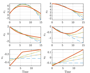
Figure 1: State and control during successive solutions. The dashed lines are the reference $\hat{x}^{i}$ and $\hat{u}^{i}$, and the solid lines are the mean state and control after the $i$^th step, $\bar{x}^{i}$ and $\bar{u}^{i}$. The first iteration is shown in blue and the final iteration is shown in bold.

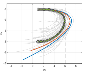
Figure 2: Successive iterations are shown by colored lines, with the initial iteration in blue. The chance constraint is shown by the black dashed line, and 90% confidence ellipses are shown in black and gray. The black confidence ellipses are computed from the linear analysis and the gray ellipses are computed from Monte Carlo, the dark gray and light gray trajectories are a subset of the Monte Carlo trails for closed and open-loop control, respectively.

VI CONCLUSION

In this paper we presented an algorithmic solution to the chance constrained nonlinear CS problem. We began by approximating the original nonlinear stochastic system by a linear discrete stochastic system, and then we formulated the linear CS problem as a deterministic optimization problem. Next, in order for the linearized problem formulation to be a reasonable approximation of the original nonlinear problem, we constrained the trajectory at each iteration within a probabilistic trust region about the trajectory from the previous iteration. The size of the trust region depends on the nonlinearity of the dynamics, and therefore convergence properties are problem-specific.

Since the proposed iCS algorithm linearizes the dynamics at each iteration, an initial trajectory must be given for the first iteration of the algorithm. At the same time, the difference in the trajectories between iterations is constrained within a trust region, and so a poor initialization may cause the first step to be infeasible. In the numerical example we addressed this problem by relaxing the chance constraints in the first iterations of the algorithm. Since the chance constrained region is assumed to be a convex polytope, the region can be easily expanded by scaling the inequality constraints. Another solution would be to first solve a deterministic optimization problem with tightened inequality constraints representing a worst-case chance constrained region. In this case, the iCS algorithm would be used to improve the solution from the deterministic problem by adding the closed-loop system statistics to the optimization. The latter approach could be applied to problems such as planetary entry and powered descent by iterating on a given reference trajectory that is to be tracked in the presence of uncertainty.

In future work we plan to apply iCS to problems in entry, descent, and landing (EDL) with nonlinear dynamics, such as entry and powered descent [21]. Another extension to this work would be the addition of time-varying chance constraints that are satisfied for all time, rather than for each time, while not being overly conservative.

References

- [1] R. Brockett, “Notes on the control of the Liouville equation,” in Control of Partial Differential Equations, Lecture Notes in Mathematics 2048, (Berlin ; New York), Springer, 2010.
- [2] A. Charnes and W. W. Cooper, “Deterministic equivalents for optimizing and satisficing under chance constraints,” Operations Research, vol. 11, no. 1, pp. 18–39, 1963.
- [3] A. Nemirovski and A. Shapiro, “Convex approximations of chance constrained programs,” SIAM Journal on Optimization, vol. 17, no. 4, pp. 969–996, 2006.
- [4] Y. Chen, T. T. Georgiou, and M. Pavon, “Optimal steering of a linear stochastic system to a final probability distribution, Part I,” IEEE Transactions on Automatic Control, vol. 61, pp. 1158–1169, May 2016.
- [5] Y. Chen, T. T. Georgiou, and M. Pavon, “Optimal steering of a linear stochastic system to a final probability distribution, Part II,” IEEE Transactions on Automatic Control, vol. 61, pp. 1170–1180, May 2016.
- [6] Y. Chen, T. T. Georgiou, and M. Pavon, “Optimal steering of a linear stochastic system to a final probability distribution, Part III,” IEEE Transactions on Automatic Control, vol. 63, pp. 3112 – 3118, August 2016.
- [7] M. Goldshtein and P. Tsiotras, “Finite-horizon covariance control of linear time-varying systems,” in IEEE 56th Annual Conference on Decision and Control, (Melbourne, Australia), pp. 3606–3611, December 2017.
- [8] K. Okamoto, M. Goldshtein, and P. Tsiotras, “Optimal covariance control for stochastic systems under chance constraints,” IEEE Control Systems Letters, vol. 2, pp. 266–271, April 2018.
- [9] K. Okamoto and P. Tsiotras, “Optimal stochastic vehicle path planning using covariance steering,” IEEE Robotics and Automation Letters, vol. 4, no. 3, pp. 2276–2281, 2019.
- [10] E. Theodorou, Y. Tassa, and E. Todorov, “Stochastic differential dynamic programming,” in American Control Conference, pp. 1125–1132, 2010.
- [11] E. Todorov and W. Li, “A generalized iterative LQG method for locally-optimal feedback control of constrained nonlinear stochastic systems,” in American Control Conference, pp. 300–306, 2005.
- [12] M. Szmuk and B. Açıkmeşe, “Successive convexification for 6-dof Mars rocket powered landing with free-final-time,” in 2018 AIAA Guidance, Navigation, and Control Conference, no. AIAA 2018-0617, 2018.
- [13] W. H. Fleming and R. W. Rishel, Deterministic and Stochastic Optimal Control. Applications of Mathematics 1, Springer-Verlag, 1975.
- [14] E. Bakolas, “Optimal covariance control for discrete-time stochastic linear systems subject to constraints,” in IEEE 55th Annual Conference on Decision and Control, (Las Vegas, NV), pp. 1153–1158, December 2016.
- [15] L. Blackmore and M. Ono, “Convex chance constrained predictive control without sampling,” in AIAA Guidance, Navigation, and Control Conference, no. AIAA 2009-5876, (Chicago, Illinois), August 2009.
- [16] M. Ono and B. C. Williams, “Iterative risk allocation: A new approach to robust model predictive control with a joint chance constraint,” in IEEE 47th Conference on Decision and Control, (Cancún, Mexico), pp. 3427–3432, December 2008.
- [17] M. P. Vitus and C. J. Tomlin, “Closed-loop belief space planning for linear, gaussian systems,” in IEEE International Conference on Robotics and Automation, (Shanghai, China), pp. 2152–2159, May 9 – 13, 2011.
- [18] Y. Ma, S. Vichik, and F. Borrelli, “Fast stochastic MPC with optimal risk allocation applied to building control systems,” in IEEE Conference on Decision and Control, (Maui, HI), pp. 7559–7564, December 2012.
- [19] M. Szmuk, B. Açıkmeşe, and A. W. Berning, “Successive convexification for fuel-optimal powered landing with aerodynamic drag and non-convex constraints,” in AIAA Guidance, Navigation, and Control Conference, no. AIAA 2016-0378, 2016.
- [20] Y. Mao, M. Szmuk, and B. Açıkmeşe, “Successive convexification of non-convex optimal control problems and its convergence properties,” in IEEE 55th Conference on Decision and Control, (Las Vegas, NV), pp. 3636–3641, December 2016.
- [21] J. Ridderhof and P. Tsiotras, “Minimum-fuel powered descent in the presence of random disturbances,” in 2019 AIAA Guidance, Navigation, and Control Conference, no. AIAA 2019-0646, (San Diego, California), 2019.
- [22] W. Li and E. Todorov, “Iterative linearization methods for approximately optimal control and estimation of non-linear stochastic system,” International Journal of Control, vol. 80, no. 9, pp. 1439–1453, 2007.
- [23] M. Ono and B. C. Williams, “An efficient motion planning algorithm for stochastic dynamic systems with constraints on probability of failure,” in AAAI, (Chicago, Illinois), pp. 1376–1382, July 2008.
- [24] M. Szmuk, T. Reynolds, B. Açıkmeşe, M. Mesbahi, and J. M. Carson, “Successive convexification for 6-dof powered descent guidance with compound state-triggered constraints,” in AIAA Scitech 2019 Forum, no. AIAA 2019-0926, 2019.
- [25] J. Ridderhof and P. Tsiotras, “Uncertainty quantification and control during Mars powered descent and landing using covariance steering,” in 2018 AIAA Guidance, Navigation, and Control Conference, no. AIAA 2018-0611, (Kissimmee, Flordia), 2018.