Classifying Partially Labeled Networked Data via Logistic Network Lasso

Abstract

We apply the network Lasso to classify partially labeled data points which are characterized by high-dimensional feature vectors. In order to learn an accurate classifier from limited amounts of labeled data, we borrow statistical strength, via an intrinsic network structure, across the dataset. The resulting logistic network Lasso amounts to a regularized empirical risk minimization problem using the total variation of a classifier as a regularizer. This minimization problem is a non-smooth convex optimization problem which we solve using a primal-dual splitting method. This method is appealing for big data applications as it can be implemented as a highly scalable message passing algorithm.

I Introduction

The least absolute shrinkage and selection operator (Lasso) has been extended to networked data recently. This extension, coined the “network Lasso” (nLasso), allows efficient processing of massive datasets using convex optimization methods [1].

Most of the existing work on nLasso-based methods focuses on predicting numeric labels (or target variables) within regression problems [2, 3, 4, 1, 5, 6, 7]. In contrast, we apply nLasso to binary classification problems which assign binary-valued labels to data points [8, 9, 10].

In order to learn a classifier from partially labeled networked data, we minimize the logistic loss incurred on a training set constituted by few labeled nodes. Moreover, we aim at learning classifiers which conform to the intrinsic network structure of the data. In particular, we require classifiers to be approximately constant over well-connected subsets (clusters) of data points. This cluster assumption lends naturally to regularized empirical risk minimization with the total variation of the classifier as regularization term [11]. We solve this non-smooth convex optimization problem by applying the primal-dual method proposed in [12, 13].

The proposed classification method extends the toolbox for semi-supervised classification in networked data [14, 15, 16, 17, 18]. In contrast to label propagation (LP), which is based on the squared error loss, we use the logistic loss which is more suitable for classification problems. Another important difference between LP methods and nLasso is the different choice of regularizer. Indeed, LP uses the Laplacian quadratic form while the nLasso uses total variation for regularization.

Using a (probabilistic) stochastic block model for networked data, a semi-supervised classification method is obtained as an instance of belief propagation method for inference in graphical models [15]. In contrast, we assume the data (network-) structure as fixed and known. The proposed method provides a statistically well-founded alternative to graph-cut methods [16, 17, 18]. While our approach is based on a convex optimization (allowing for highly scalable implementation), graph-cuts is based on combinatorial optimization which makes scaling them to large datasets more challenging. Moreover, while graph-cut methods apply only to data which is characterized by network structure and labels, our method allows to exploit additional information provided by feature vectors of data points.

Contribution: Our main contributions are: (i) We present a novel implementation of logistic network Lasso by applying a primal-dual method. This method can be implemented as highly scalable message passing on the network structure underlying the data. (ii) We prove the convergence of this primal-dual method and (iii) verify its performance on synthetic classification problems in chain and grid-structured data.

Notation: Boldface lowercase (uppercase) letters denote vectors (matrices). We denote $\mathbf{x}^{T}$ the transpose of vector $\mathbf{x}$. The $\ell_{2}$-norm of a vector $\mathbf{x}$ is $\|\mathbf{x}\|=\sqrt{\mathbf{x}^{T}\mathbf{x}}$. The convex conjugate of a function $f$ is defined as $f^{*}(\mathbf{y})=\sup_{\mathbf{x}}(\mathbf{y}^{T}\mathbf{x}-f(\mathbf{x}))$. We also need the sigmoid function $\sigma(z):=1/(1+\exp(-z))$.

II Problem Formulation

We consider networked data that is represented by an undirected weighted graph (the “empirical graph”) $\mathcal{G}=(\mathcal{V},\mathcal{E},\mathbf{A})$. A particular node $i\in\mathcal{V}=\{1,\ldots,N\}$ of the graph represents an individual data point (such as a document, or a social network user profile). Two different data points $i,j\in\mathcal{V}$ are connected by an undirected edge $\{i,j\}\in\mathcal{E}$ if they are considered similar (such as documents authored by the same person or social network profiles of befriended users). For ease of notation, we denote the edge set $\mathcal{E}$ by $\{1,\ldots,E:=|\mathcal{E}|\}$.

Each edge $e=\{i,j\}\in\mathcal{E}$ is endowed with a positive weight $A_{e}=A_{ij}>0$ which quantifies the amount of similarity between data points $i,j\in\mathcal{V}$. The neighborhood of a node $i\in\mathcal{V}$ is $\mathcal{N}(i):=\{j:\{i,j\}\in\mathcal{E}\}$.

Beside the network structure, datasets convey additional information in the form of features $\mathbf{x}^{(i)}\in\mathbb{R}^{d}$ and labels $y^{(i)}\in\{-1,1\}$ associated with each data point $i\in\mathcal{V}$. In what follows, we assume the features to be normalized such that $\|\mathbf{x}^{(i)}\|=1$ for each data points $i\in\mathcal{V}$. While features are typically available for each data point $i\in\mathcal{V}$, labels are costly to acquire and available only for data points in a small training set $\mathcal{M}=\{i_{1},\ldots,i_{M}\}$ containing $M$ labeled data points.

We model the labels $y^{(i)}$ of the data points $i\in\mathcal{V}$ as independent random variables with (unknown) probabilities

$$p^{(i)}:={\rm Prob}\{y^{(i)}\!=\!1\}=\frac{1}{1+\exp(-(\mathbf{w}^{(i)})^{T}\mathbf{x}^{(i)})}.$$ (1)

The probabilities $\{p^{(i)}\}_{i\in\mathcal{V}}$ are parametrized by some (unknown) weight vectors $\mathbf{w}^{(i)}$. Our goal is to develop a method for learning an accurate estimate $\widehat{\mathbf{w}}^{(i)}$ of the weight vector $\mathbf{w}^{(i)}$. Given the estimate $\widehat{\mathbf{w}}^{(i)}$, we can compute an estimate $\hat{p}^{(i)}$ for the probability $p^{(i)}$ by replacing ${\mathbf{w}}^{(i)}$ with $\widehat{\mathbf{w}}^{(i)}$ in (1).

We interpret the weight vectors as the values of a graph signal $\mathbf{w}:\mathcal{V}\rightarrow\mathbb{R}^{d}$ assigning each node $i\in\mathcal{V}$ of the empirical graph $\mathcal{G}$ the vector $\mathbf{w}^{(i)}\in\mathbb{R}^{d}$. The set of all vector-valued graph signals is denoted $\mathcal{C}\!:=\!\{\mathbf{w}:\mathcal{V}\rightarrow\mathbb{R}^{d}:i\mapsto\mathbf{w}^{(i)}\}$.

Each graph signal $\widehat{\mathbf{w}}\in\mathcal{C}$ defines a classifier which maps a node with features $\mathbf{x}^{(i)}$ to the predicted label

$$\widehat{y}^{(i)}=\begin{cases}1&\text{if }\big{(}\widehat{\mathbf{w}}^{(i)}\big{)}^{T}\mathbf{x}^{(i)}>0\\ -1&{\rm otherwise}.\end{cases}$$ (2)

Given partially labeled networked data, we aim at leaning a classifier $\widehat{\mathbf{w}}\in\mathcal{C}$ which agrees with the labels $y^{(i)}$ of labeled data points in the training set $\mathcal{M}$. In particular, we aim at learning a classifier having a small training error

$$\widehat{E}(\widehat{\mathbf{w}})\!:=\!({1}/{M})\sum_{i\in\mathcal{M}}\!\ell((\widehat{\mathbf{w}}^{(i)})^{T}\widetilde{\mathbf{x}}^{(i)})$$ (3)

with $\widetilde{\mathbf{x}}^{(i)}:=y^{(i)}\mathbf{x}^{(i)}$ and the logistic loss

$$\ell(z):={\rm log}(1+\exp(-z))=-{\rm log}(\sigma(z)).\vspace*{-3mm}$$ (4)

III Logistic Network Lasso

The criterion (3) by itself is not enough for guiding the learning of a classifier $\mathbf{w}$ since (3) completely ignores the weights $\widehat{\mathbf{w}}^{(i)}$ at unlabeled nodes $i\in\mathcal{V}\setminus\mathcal{M}$. Therefore, we need to impose some additional structure on the classifier $\widehat{\mathbf{w}}$. In particular, any reasonable classifier $\widehat{\mathbf{w}}$ should conform with the cluster structure of the empirical graph $\mathcal{G}$ [19].

We measure the extend of a classifier $\widehat{\mathbf{w}}\in\mathcal{C}$ conforming with the cluster structure of $\mathcal{G}$ by the total variation (TV)

$$\|\mathbf{w}\|_{\rm TV} :=\sum_{\{i,j\}\in\mathcal{E}}A_{ij}\|\mathbf{w}^{(j)}-\mathbf{w}^{(i)}\|.$$ (5)

A classifier $\widehat{\mathbf{w}}\!\in\!\mathcal{C}$ has small TV if the weights $\widehat{\mathbf{w}}^{(i)}$ are approximately constant over well connected subsets (clusters) of nodes.

We are led quite naturally to learning a classifier $\widehat{\mathbf{w}}$ via the regularized empirical risk minimization (ERM)

$$\widehat{\mathbf{w}} \in\operatorname*{argmin}_{\mathbf{w}\in\mathcal{C}}\widehat{E}(\mathbf{w})+\lambda\|\mathbf{w}\|_{\rm TV}.$$ (6)

We refer to (6) as the logistic nLasso (lnLasso) problem. The parameter $\lambda$ in (6) allows to trade-off small TV $\|\widehat{\mathbf{w}}\|_{\rm TV}$ against small error $\widehat{E}(\widehat{\mathbf{w}})$ (cf. (3)). The choice of $\lambda$ can be guided by cross validation [20].

Note that lnLasso (6) does not enforce directly the labels $y^{(i)}$ to be clustered. Instead, it requires the classifier $\widehat{\mathbf{w}}$, which parametrizes the probability distributed of the labels $y^{(i)}$ (see (1)), to be clustered.

It will be convenient to reformulate (6) using vector notation. We represent a graph signal $\mathbf{w}\in\mathcal{C}$ as the vector

$$\mathbf{w}=((\mathbf{w}^{(1)})^{T},\ldots,(\mathbf{w}^{(N)})^{T})^{T}\in\mathbb{R}^{dN}.$$ (7)

Define a partitioned matrix $\mathbf{D}\in\mathbb{R}^{(dE)\times(dN)}$ block-wise as

$$\mathbf{D}_{e,i}=\begin{cases}A_{ij}\mathbf{I}_{d}&e=\{i,j\},i<j\\ -A_{ij}\mathbf{I}_{d}&e=\{i,j\},i>j\\ \mathbf{0}&{\rm otherwise},\end{cases}$$ (8)

where $\mathbf{I}_{d}\in\mathbb{R}^{d\times d}$ is the identity matrix. The term $A_{ij}(\mathbf{w}^{(i)}-\mathbf{w}^{(j)})$ in (5) is the $e$-th block of $\mathbf{D}\mathbf{w}$. Using (7) and (8), we can reformulate the lnLasso (6) as

$$\widehat{\mathbf{w}}\in\operatorname*{argmin}_{\mathbf{w}\in\mathbb{R}^{dN}}h(\mathbf{w})+g(\mathbf{D}\mathbf{w}),$$ (9)

with

$$h(\mathbf{w})=\widehat{E}(\mathbf{w})\text{ and }g(\mathbf{u}):=\lambda\sum_{e=1}^{E}\|\mathbf{u}^{(e)}\|$$ (10)

with stacked vector $\mathbf{u}=(\mathbf{u}^{(1)},\ldots,\mathbf{u}^{(E}))\in\mathbb{R}^{dE}$.

IV primal-dual method

The lnLasso (9) is a convex optimization problem with a non-smooth objective function which rules out the use of gradient descent methods [21]. However, the objective function is highly structured since it is the sum of a smooth convex function $h(\mathbf{w})$ and a non-smooth convex function $g(\mathbf{D}\mathbf{w})$, which can be optimized efficiently when considered separately. This suggests to use a proximal splitting method [22, 23, 12] for solving (9). One particular such method is the preconditioned primal-dual method [24] which is based on reformulating the problem (9) as a saddle-point problem

$$\min_{\mathbf{w}\in\mathbb{R}^{dN}}\max_{\mathbf{u}\in\mathbb{R}^{dE}}\mathbf{u}^{T}\mathbf{D}\mathbf{w}+h(\mathbf{w})-g^{*}(\mathbf{u}),$$ (11)

with the convex conjugate $g^{*}$ of $g$ [12].

Solutions $(\widehat{\mathbf{w}},\widehat{\mathbf{u}})$ of (11) are characterized by [25, Thm 31.3]

$$-\mathbf{D}^{T}\widehat{\mathbf{u}}\in\partial h(\widehat{\mathbf{w}})$$

$$\mathbf{D}\widehat{\mathbf{w}}\in\partial g^{*}(\widehat{\mathbf{u}}).$$ (12)

This condition is, in turn, equivalent to

$$\widehat{\mathbf{w}}-\mathbf{T}\mathbf{D}^{T}\widehat{\mathbf{u}}\in(\mathbf{I}_{dN}+\mathbf{T}\partial h)(\widehat{\mathbf{w}}),$$

$$\widehat{\mathbf{u}}+\bm{\Sigma}\mathbf{D}\widehat{\mathbf{w}}\in(\mathbf{I}_{dE}+\bm{\Sigma}\partial g^{*})(\widehat{\mathbf{u}}),$$ (13)

with positive definite matrices $\bm{\Sigma}\!\in\!\mathbb{R}^{dE\times dE},\mathbf{T}\!\in\!\mathbb{R}^{dN\times dN}$. The matrices $\bm{\Sigma},\mathbf{T}$ are design parameters whose choice will be detailed below. The condition (13) lends naturally to the following coupled fixed point iterations [24]

$$\mathbf{w}_{k+1}\! =\!(\mathbf{I}\!+\!\mathbf{T}\partial h)^{-1}(\mathbf{w}_{k}\!-\!\mathbf{T}\mathbf{D}^{T}\mathbf{u}_{k})$$ (14)

$$\mathbf{u}_{k+1}\! =\!(\mathbf{I}\!+\!\bm{\Sigma}\partial g^{*})^{-1}(\mathbf{u}_{k}\!+\!\bm{\Sigma}\mathbf{D}(2\mathbf{w}_{k+1}\!-\!\mathbf{w}_{k})).$$ (15)

The update (15) involves the resolvent operator

$$(\mathbf{I}\!+\!\bm{\Sigma}\partial g^{*})^{-1}(\mathbf{v})\!=\!\operatorname*{argmin}_{\mathbf{v}^{\prime}\in\mathbb{R}^{dE}}g^{*}(\mathbf{v}^{\prime})\!+\!(1/2)\|\mathbf{v}^{\prime}\!-\!\mathbf{v}\|^{2}_{\bm{\Sigma}^{-1}},$$ (16)

where $\|\mathbf{v}\|_{\bm{\Sigma}}\!:=\!\sqrt{\mathbf{v}^{T}\Sigma\mathbf{v}}$. The convex conjugate $g^{*}$ of $g$ (see (10)) can be decomposed as $g^{*}(\mathbf{v})=\sum_{e=1}^{E}g_{2}^{*}(\mathbf{v}^{(e)})$ with the convex conjugate $g_{2}^{*}$ of the scaled $\ell_{2}$-norm $\lambda\|.\|$. Moreover, since $\bm{\Sigma}$ is a block diagonal matrix, the $e$-th block of the resolvent operator $(\mathbf{I}_{dE}+\bm{\Sigma}\partial g^{*})^{-1}(\mathbf{v})$ can be obtained by the Moreau decomposition as [26, Sec. 6.5]

$$((\mathbf{I}_{dE}+\bm{\Sigma}\partial g^{*})^{-1}(\mathbf{v}))^{(e)}$$

$$\stackrel{{\scriptstyle\eqref{equ_def_prox}}}{{=}}\operatorname*{argmin}_{\mathbf{v}^{\prime}\in\mathbb{R}^{d}}g_{2}^{*}(\mathbf{v}^{\prime})\!+\!(1/(2\sigma^{(e)}))\|\mathbf{v}^{\prime}\!-\!\mathbf{v}^{(e)}\|^{2}$$

$$=\mathbf{v}^{(e)}\!-\!\sigma^{(e)}(\mathbf{I}_{d}\!+\!(\lambda/\sigma^{(e)})\partial\|.\|)^{-1}(\mathbf{v}^{(e)}/\sigma^{(e)})$$

$$=\begin{cases}\lambda\mathbf{v}^{(e)}/\|\mathbf{v}^{(e)}\|&\text{if }\|\mathbf{v}^{(e)}\|>\lambda\\ \mathbf{v}^{(e)}&{\rm otherwise},\end{cases}$$

where $(a)_{+}\!=\!\max\{a,0\}$ for $a\in\mathbb{R}$.

The update (14) involves the resolvent operator $(\mathbf{I}+\mathbf{T}\partial h)^{-1}$ of $h$ (see (3) and (10)), which does not have a closed-form solution. Choosing $\mathbf{T}\!=\!{\rm diag}\{\tau^{(i)}\mathbf{I}_{d}\}_{i=1}^{N}$, we can solve (14) approximately by a simple iterative method [27, Sec. 8.2]. Setting$\overline{\mathbf{w}}\!:=\!\mathbf{w}_{k}\!-\!\mathbf{T}\mathbf{D}^{T}\mathbf{u}_{k}$, the update (14) becomes

$$\mathbf{w}^{(i)}_{k+1}\!:=\!\operatorname*{argmin}_{\widetilde{\mathbf{w}}\in\mathbb{R}^{d}}2\ell(\widetilde{\mathbf{w}}^{T}\widetilde{\mathbf{x}}^{(i)})\!+\!(M/\tau^{(i)})\!\|\widetilde{\mathbf{w}}\!-\!\overline{\mathbf{w}}^{(i)}\|^{2}.$$ (17)

If the matrices $\bm{\Sigma}$ and $\mathbf{T}$ satisfy

$$\|\bm{\Sigma}^{1/2}\mathbf{D}\mathbf{T}^{1/2}\|^{2}<1,$$ (18)

the sequences obtained from iterating (14) and (15) converge to a saddle point of the problem (11) [24, Thm. 1]. The condition (18) is satisfied for the choice $\bm{\Sigma}=\{(1/(2A_{e}))\mathbf{I}_{d}\}_{e\in\mathcal{E}}$ and $\{(\tau/d^{(i)})\mathbf{I}_{d}\}_{i\in\mathcal{V}}$, with node degree $d^{(i)}=\sum_{j\neq i}A_{ij}$ and some $\tau<1$ [24, Lem. 2].

Solving (17) is equivalent to the zero-gradient condition

$${-\widetilde{\mathbf{x}}^{(i)}\sigma(-(\mathbf{w}^{(i)})^{T}\widetilde{\mathbf{x}}^{(i)})}+(M/\tau^{(i)})({\mathbf{w}^{(i)}}\!-\!\overline{\mathbf{w}}^{(i)})=0.$$ (19)

The solutions of (19) are fixed-points of the map

$${\bf\Phi}^{(i)}(\mathbf{u})=\overline{\mathbf{w}}^{(i)}+(\tau^{(i)}/M){\widetilde{\mathbf{x}}^{(i)}\sigma(-\mathbf{u}^{T}\widetilde{\mathbf{x}}^{(i)})}.$$ (20)

Lemma 1.

The mapping ${\bf\Phi}^{(i)}$ (20) is Lipschitz with constant $\beta_{i}=\tau^{(i)}\|\mathbf{x}^{(i)}\|^{2}/M$.

Proof.

For any $a,b\in\mathbb{R}$,

$$\big{|}1/({1+\exp(a)})\!-\!{1}/({1\!+\!\exp(b)})\big{|}\leq|a\!-\!b|$$

which implies

$$\big{|}\sigma(-\mathbf{u}^{T}\widetilde{\mathbf{x}}^{(i)}) \!-\!\sigma(-\mathbf{v}^{T}\widetilde{\mathbf{x}}^{(i)})\big{|}\leq\|\mathbf{x}^{(i)}\|\|\mathbf{u}-\mathbf{v}\|,$$

and, in turn,

$$\|{\bf\Phi}^{(i)}(\mathbf{u})-{\bf\Phi}^{(i)}(\mathbf{v})\| \stackrel{{\scriptstyle}}{{\leq}}(\tau^{(i)}\|\widetilde{\mathbf{x}}^{(i)}\|/M)\|\mathbf{x}^{(i)}\|\|\mathbf{u}-\mathbf{v}\|$$

$$=\beta_{i}\|\mathbf{u}-\mathbf{v}\|.$$

∎

We approximate the exact update (17) with

$$\widehat{\mathbf{w}}_{k+1}^{(i)}=\underbrace{{\bf\Phi}^{(i)}\circ\ldots\circ{\bf\Phi}^{(i)}}_{\lceil 2\log(k)/\log(1/\beta_{i})\rceil}(\overline{\mathbf{w}}^{(i)}).$$ (21)

According to [28, Thm. 1.48], for $\tau^{(i)}\!<\!M/\|\mathbf{x}^{(i)}\|^{2}$ the error incurred by replacing (17) with (21) satisfies

$$e_{k}=\|\widehat{\mathbf{w}}_{k+1}^{(i)}-{\mathbf{w}}_{k+1}^{(i)}\|\leq 1/k^{2}.$$ (22)

Given the error bound (22), as can be verified using [13, Thm. 3.2], the sequences obtained by (14) and (15) when replacing the exact update (17) with (21) converge to a saddle-point of (11) and, in turn, a solution of lnLasso (9).

Algorithm 1 lnLasso via primal-dual method

1:$\mathcal{G}=(\mathcal{V},\mathcal{E},\mathbf{A})$, $\{\mathbf{x}^{(i)}\}_{i\in\mathcal{V}}$, $\mathcal{M}$, $\{y^{(i)}\}_{i\in\mathcal{M}}$, $\lambda$, $\mathbf{D}$, $\bm{\Sigma}={\rm diag}\{\sigma^{(e)}=1/(2A_{e})\mathbf{I}_{d}\}_{e=1}^{E}$, $\mathbf{T}={\rm diag}\{\tau^{(i)}=0.9/d^{(i)}\mathbf{I}_{d}\}_{i\in\mathcal{V}}$, $\beta_{i}=\tau^{(i)}/|\mathcal{M}|$

2:Initialize: $k\!:=\!0$, $\widehat{\mathbf{w}}_{0}\!:=\!0$, $\widehat{\mathbf{u}}_{0}\!:=\!0$

3:repeat

4:     $\widehat{\mathbf{w}}_{k+1}:=\widehat{\mathbf{w}}_{k}-\mathbf{T}\mathbf{D}^{T}\widehat{\mathbf{u}}_{k}$

5:     for  each labeled node $i\in\mathcal{M}$ do

6:         

$$\widehat{\mathbf{w}}_{k+1}^{(i)}:=\underbrace{{\bf\Phi}^{(i)}\circ\ldots\circ{\bf\Phi}^{(i)}}_{\lceil 2\log(k)/\log(1/\beta_{i})\rceil}(\widehat{\mathbf{w}}_{k+1}^{(i)})$$

7:     end for

8:     $\overline{\mathbf{u}}:={\mathbf{u}}_{k}+\bm{\Sigma}\mathbf{D}(2\widehat{\mathbf{w}}_{k+1}-\widehat{\mathbf{w}}_{k})$

9:     $\widehat{\mathbf{u}}_{k+1}^{(e)}=\overline{\mathbf{u}}^{(e)}-\bigg{(}1-\frac{\lambda}{\|\overline{\mathbf{u}}^{(e)}\|}\bigg{)}_{+}\overline{\mathbf{u}}^{(e)}$ for $e\in\mathcal{E}$

10:     $k\!:=\!k\!+\!1$

11:until stopping criterion is satisfied

12:$(\widehat{\mathbf{w}}_{k},\widehat{\mathbf{u}}_{k})$.

V Numerical Experiments

We assess the performance of lnLasso Alg. 1 on datasets whose empirical graph is either a chain graph or a grid graph.

V-A Chain

For this experiment, we generate a dataset whose empirical graph is a chain consisting of $N\!=\!400$ nodes which represent individual data points. The chain graph is partitioned into 8 clusters, $\mathcal{C}_{r}=\{r\cdot 50+1,\ldots,r\cdot 50+50\}$, for $r=0,\ldots 7$. The edge weights $A_{ij}$ are set to $100$ if nodes $i$ and $j$ belong to the same cluster and $1$ otherwise.

All nodes $i\in\mathcal{C}_{r}$ in a particular cluster $\mathcal{C}_{r}$ share the same weight vector $\mathbf{w}^{(r)}\sim\mathcal{N}(0,\mathbf{I})$ which is generated from a standard normal distribution. The feature vectors $\mathbf{x}^{(i)}\in\mathbb{R}^{3}$ are generated i.i.d. using a uniform distribution over $[0,1]^{3}$. The true node labels $y^{(i)}$ are drawn from the distribution (1). The training set is obtained by independently selecting each node with probability (labeling rate) $p$.

We apply Alg. 1 to obtain a classifier $\widehat{\mathbf{w}}$ which allows to classify data points as $\widehat{y}^{(i)}={\rm sign}((\widehat{\mathbf{w}}^{(i)})^{T}\mathbf{x}^{(i)})$. In order to assess the performance of Alg. 1 we compute the accuracy within the unlabeled nodes, i.e., the ratio of the number of correct labels achieved by Alg. 1 for unlabeled nodes to the number of unlabeled nodes,

$$ACC:=\big{(}1/({N-M})\big{)}{|\{i:y^{(i)}=\widehat{y}{}^{(i)},i\notin\mathcal{M}\}|}.\vspace{-3mm}$$ (23)

We compute the accuracy of Alg. 1 for different choices of $p\in\{0.1,\ldots,0.9\}$ and $\lambda\in\{10^{-5},\ldots,10^{-1}\}$. For a pair of $\{\lambda,p\}$, we repeat the experiment $100$ times and compute the average accuracy.

The accuracies obtained for varying labeling rates $p$ and lnLasso parameter $\lambda$ is plotted in Fig. 1. As indicated in Fig. 1, the accuracy increases with labeling rate $p$ which confirms the intuition that increasing the amount of labeled data (training set size) supports the learning quality.

The accuracies in Fig. 1 are low since the classifier assigns the labels to nodes based on (2) while the true labels are drawn from the probabilistic model (1). Indeed, we also plot in Fig. 1 the optimal accuracy, determined by the average of the probability to assign nodes $i$ to their true label when knowing $p^{(i)}$ using (1), as a horizontal dashed line. Fig. 1 shows that accuracies increase with labeling rate $p$ and tends toward the optimal accuracy.

Figure 1: The classification accuracy for chain-structured data.

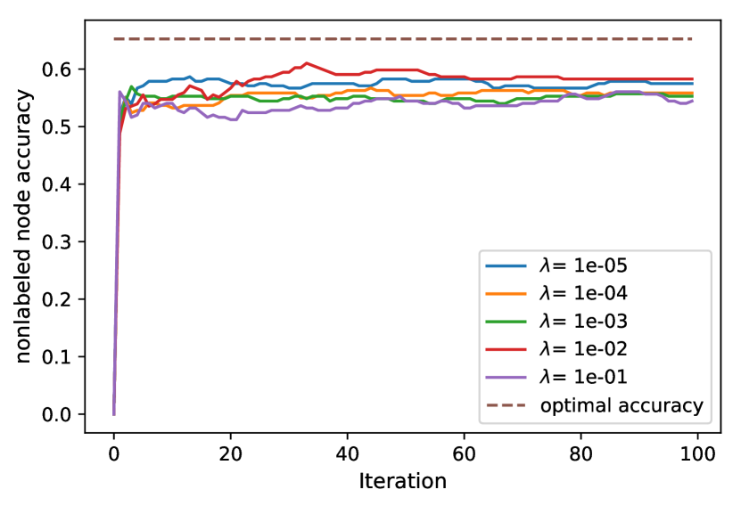
Figure 2: The convergence rate of Alg. 1 for chain structured data and labeling rate $p=0.4$.

In Fig. 2, we plot the accuracy (cf. (23)) as a function of the number of iterations used in Alg. 1 for varying lnLasso parameter $\lambda$ and fixed labeling rate $p\!=\!4/10$. Fig. 2 illustrates that, for a larger value of $\lambda$, e.g. $\lambda=10^{-1}$ or $10^{-2}$, Alg. 1 tends to deliver a classifier with better accuracy than that of smaller $\lambda$, e.g. $\lambda=10^{-4}$ or $10^{-5}$. This proves that taking into account the network structure is beneficial to classify a networked data. Moreover, it is shown in Fig. 2 that the accuracies do not improve after few iterations. This implies that lnLasso can yields a reasonable accuracy after a few number of iterations.

V-B Grid

In the second experiment, we consider a grid graph with $N=20\!\times\!20\!=\!400$ nodes. The graph is partitioned into $4$ clusters which are grid graphs of size $10\times 10$. Similar to the chain, the edge weights $A_{ij}=100$ if nodes $i$ and $j$ belong to the same cluster and $A_{ij}=1$ otherwise. The average accuracies are plotted in Fig. 3 which also shows that the accuracy increases with the labeling rate $p$. We also plot the accuracy (cf. (23)) over iterations of Alg. 1 for different values of $\lambda$ with $p=0.4$ in Fig. 4.

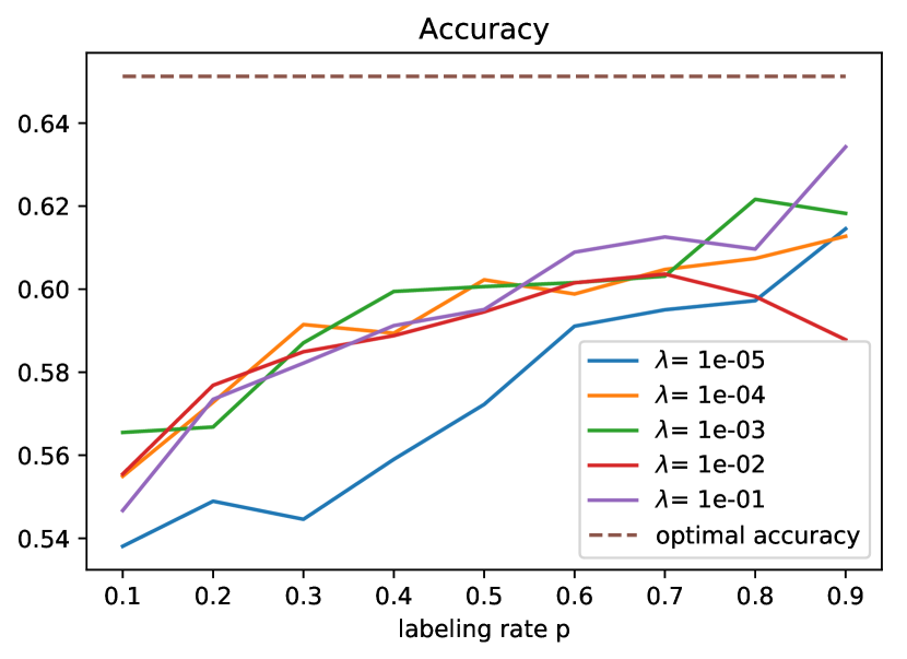
Figure 3: The classification accuracy for grid-structured data.

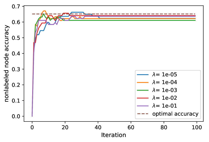
Figure 4: The convergence rate of Alg. 1 for grid structured data and labeling rate $p=0.4$.

References

- [1] D. Hallac, J. Leskovec, and S. Boyd, “Network lasso: Clustering and optimization in large graphs,” in Proc. SIGKDD, 2015, pp. 387–396.
- [2] A. Jung, N.T. Quang, and A. Mara, “When is network lasso accurate?,” Frontiers in Appl. Math. and Stat., vol. 3, pp. 28, 2018.
- [3] M. Yamada, T. Koh, T. Iwata, J.S. Taylor, and S. Kaski, “Localized Lasso for High-Dimensional Regression,” in Proceedings of the 20th International Conference on Artificial Intelligence and Statistics, Aarti Singh and Jerry Zhu, Eds., Fort Lauderdale, FL, USA, 20–22 Apr 2017, vol. 54 of Proceedings of Machine Learning Research, pp. 325–333, PMLR.
- [4] A. Jung and M. Hulsebos, “The network nullspace property for compressed sensing of big data over networks,” Front. Appl. Math. Stat., Apr. 2018.
- [5] S. Chen, A. Sandryhaila, J. M. F. Moura, and J. Kovačević, “Signal recovery on graphs: Variation minimization,” IEEE Trans. Signal Processing, vol. 63, no. 17, pp. 4609–4624, Sept. 2015.
- [6] A. Sandryhaila and J. M. F. Moura, “Big data analysis with signal processing on graphs: Representation and processing of massive data sets with irregular structure,” IEEE Signal Processing Magazine, vol. 31, no. 5, pp. 80–90, Sept 2014.
- [7] A. Jung, “On the complexity of sparse label propagation,” Front. Appl. Math. Stat., Jul. 2018.
- [8] S. Bhagat, C. Graham, and S. Muthukrishnan, Social network data analytics, Springer, 2011.
- [9] L. Lovász, Large Networks and Graph Limits, American Mathematical Society, 2012.
- [10] S. Cui, A. Hero, Z.-Q. Luo, and J.M.F. Moura, Eds., Big Data over Networks, Cambridge Univ. Press, 2016.
- [11] V. N. Vapnik, The Nature of Statistical Learning Theory, Springer, 1999.
- [12] A. Chambolle and T. Pock, “A first-order primal-dual algorithm for convex problems with applications to imaging,” J. Math. Imaging Vision, vol. 40, no. 1, pp. 120–145, 2011.
- [13] L. Condat, “A primal–dual splitting method for convex optimization involving lipschitzian, proximable and linear composite terms,” Journal of Optimization Theory and Applications, vol. 158, no. 2, pp. 460–479, Aug 2013.
- [14] O. Chapelle, B. Schölkopf, and A. Zien, Eds., Semi-Supervised Learning, The MIT Press, Cambridge, Massachusetts, 2006.
- [15] Pan Zhang, Cristopher Moore, and Lenka Zdeborová, “Phase transitions in semisupervised clustering of sparse networks,” Physical review. E, Statistical, nonlinear, and soft matter physics, vol. 90 5-1, pp. 052802, 2014.
- [16] P. Ruusuvuori, T. Manninen, and H. Huttunen, “Image segmentation using sparse logistic regression with spatial prior,” in 2012 Proceedings of the 20th European Signal Processing Conference (EUSIPCO), Aug. 2012, pp. 2253–2257.
- [17] R. K chichian, S. Valette, and M. Desvignes, “Automatic multiorgan segmentation via multiscale registration and graph cut,” IEEE Transactions on Medical Imaging, vol. 37, no. 12, pp. 2739–2749, Dec 2018.
- [18] Y. Boykov and V. Kolmogorov, “An experimental comparison of min-cut/max- flow algorithms for energy minimization in vision,” IEEE Transactions on Pattern Analysis and Machine Intelligence, vol. 26, no. 9, pp. 1124–1137, Sept. 2004.
- [19] M. E. J. Newman, Networks: An Introduction, Oxford Univ. Press, 2010.
- [20] T. Hastie, R. Tibshirani, and J. Friedman, The Elements of Statistical Learning, Springer Series in Statistics. Springer, New York, NY, USA, 2001.
- [21] A. Jung, “A fixed-point of view on gradient methods for big data,” Frontiers in Applied Mathematics and Statistics, vol. 3, pp. 18, 2017.
- [22] P. L. Combettes and J.-C. Pesquet, “Proximal Splitting Methods in Signal Processing,” ArXiv e-prints, Dec. 2009.
- [23] D. O’Connor and L. Vandenberghe, “Primal-dual decomposition by operator splitting and applications to image deblurring,” SIAM Journal on Imaging Sciences, vol. 7, no. 3, pp. 1724–1754, 2014.
- [24] T. Pock and A. Chambolle, “Diagonal preconditioning for first order primal-dual algorithms in convex optimization,” in IEEE International Conference on Computer Vision (ICCV), Nov 2011, pp. 1762–1769.
- [25] R. T. Rockafellar, Convex Analysis, Princeton Univ. Press, Princeton, NJ, 1970.
- [26] N. Parikh and S. Boyd, “Proximal algorithms,” Foundations and Trends in Optimization, vol. 1, no. 3, pp. 123–231, 2013.
- [27] S. Boyd, N. Parikh, E. Chu, B. Peleato, and J. Eckstein, Distributed Optimization and Statistical Learning via the Alternating Direction Method of Multipliers, vol. 3 of Foundations and Trends in Machine Learning, Now Publishers, Hanover, MA, 2010.
- [28] H. H. Bauschke and P. L. Combettes, Convex Analysis and Monotone Operator Theory in Hilbert Spaces, Springer, New York, 2011.