Maintaining the Union of Unit Discs under Insertions with Near-Optimal Overhead

Abstract

We present efficient dynamic data structures for maintaining the union of unit discs and the lower envelope of pseudo-lines in the plane. More precisely, we present three main results in this paper:

• We present a linear-size data structure to maintain the union of a set of unit discs under insertions. It can insert a disc and update the union in $O((k+1)\log^{2}n)$ time, where $n$ is the current number of unit discs and $k$ is the combinatorial complexity of the structural change in the union due to the insertion of the new disc. It can also compute, within the same time bound, the area of the union after the insertion of each disc.

• We propose a linear-size data structure for maintaining the lower envelope of a set of $x$-monotone pseudo-lines. It can handle insertion/deletion of a pseudo-line in $O(\log^{2}n)$ time; for a query point $x_{0}\in\mathbb{R}$, it can report, in $O(\log n)$ time, the point on the lower envelope with $x$-coordinate $x_{0}$; and for a query point $q\in\mathbb{R}^{2}$, it can return all $k$ pseudo-lines lying below $q$ in time $O(\log n+k\log^{2}n)$.

• We present a linear-size data structure for storing a set of circular arcs of unit radius (not necessarily on the boundary of the union of the corresponding discs), so that for a query unit disc $D$, all input arcs intersecting $D$ can be reported in $O(n^{1/2+\varepsilon}+k)$ time, where $k$ is the output size and $\varepsilon>0$ is an arbitrarily small constant. A unit-circle arc can be inserted or deleted in $O(\log^{2}n)$ time.

1 Introduction

Problem statement.

Let $S=\{p_{1},\ldots,p_{n}\}$ be set of $n$ points in $\mathbb{R}^{2}$, let $D(p_{i})$ be the unit disc centered at $p_{i}$, and let $U:=U(S):=\bigcup_{p\in S}D(p)$ be the union of the unit discs centered at the points of $S$. We wish to maintain the boundary $\partial U$ of $U$, as new points are added to $S$. In particular, we wish to maintain (i) the set of edges on $\partial U$ and (ii) the area of $U$.

The efficient manipulation of collections of unit discs in the plane is a widely and frequently studied topic, e.g., in the context of sensor networks, where every disc represents the area covered by a sensor. In our setting, we are motivated by the problem of multiple agents traversing a region in search of a particular target [16]. We are interested in investigating the pace of coverage as the agents move, and we wish to estimate at each stage the overall area that has been covered so far. The simulation is discretized, i.e., each agent is modeled by a unit disc whose motion is simulated by changing its location at fixed time steps. In other words, we are receiving a stream $\{p_{1},p_{2},...,p_{i}\}$ of points in $\mathbb{R}^{2}$. When the next point $p_{i+1}$ arrives, we want to quickly compute the area of $D(p_{i+1})\setminus\bigcup_{j\leq i}D(p_{j})$.

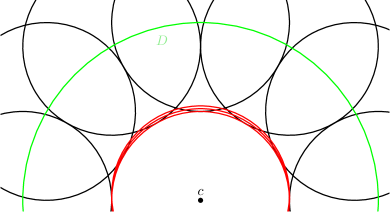
Figure 1: An instance in which the union boundary of a set of unit discs in the plane undergoes $\Omega(n^{2})$ combinatorial changes during $n$ insertions. The black discs are inserted first, and then red discs are inserted from bottom to top.

It is known that even for discs of arbitrary radii, the boundary $\partial U$ has $O(n)$ vertices and edges [24], and that $\partial U$ can be computed in $O(n\log n)$ time using power diagrams [7]. An incremental algorithm [30] can maintain $\partial U$ under $n$ insertions in total time $O(n^{2})$. This is worst-case optimal, as the total amount of structural change to $\partial U$ under a sequence of $n$ insertions can be $\Omega(n^{2})$ in the worst case. For instance, refer to Figure 1. Let $D$ be a disc of radius $2$ centered at the origin (green). We first insert $n/2$ unit discs with equidistant centers on $\partial D$ (black). Next, we insert $n/2$ (red) unit discs such that the center of the $i$th red disc is $(0,\varepsilon i)$ on the $y$-axis, for some sufficiently small constant $\varepsilon>0$. The insertion of each of the last $n/2$ discs creates $n$ vertices on the union of the discs inserted so far. Our goal is thus to develop an output-sensitive algorithm that uses $O(n)$ space and updates $U$ in time proportional to the number of changes in vertices and edges of $\partial U$ due to the insertion of a new disc.

Maintaining the edges of $\partial U$ requires answering intersection-searching queries of the following form: Given a collection $\mathscr{C}$ of unit-radius circular arcs that comprise $\partial U$ and a query unit disc $D$, report the arcs in $\mathscr{C}$ that intersect $D$. Developing an efficient data structure for this intersection-searching problem led us to study the following problem, which is interesting in its own right: A set of pseudo-lines is a set of bi-infinite simple curves in the plane such that each pair of curves intersect in exactly one point and they cross at that point. Given a set $E$ of $x$-monotone pseudo-lines in the plane, we wish to maintain their lower envelope $\mathscr{L}(E)$ (see Section 2 below for the definition) under insertions and deletions of pseudo-lines, such that for a point $x_{0}\in\mathbb{R}$, the point on $\mathscr{L}(E)$ with $x$-coordinate $x_{0}$ can be reported quickly.

Related work.

Arrangements of pseudo-lines have been studied extensively in discrete and computational geometry; see, e.g., the classic monograph by Grünbaum [18] and recent surveys [17, 20] for a review of combinatorial bounds and algorithms involving arrangements of pseudo-lines. For the case of lines (rather than pseudo-lines), the celebrated result by Overmars and van Leeuwen [27] can maintain the lower envelope in $O(\log^{2}n)$ time under insertion and deletion of lines. This bound has been improved over the last two decades [12, 13, 21, 11, 23]; these improvements are, however, not directly applicable for pseudo-lines. If only insertions are performed, then the data structure by Preparata [28] can be extended to maintain the lower envelope of a set of pseudo-lines in $O(\log n)$ time per update.

A series of papers have developed powerful general data structures for maintaining the lower envelopes of a set of curves of bounded description complexity, based on shallow cuttings [4, 14, 22, 25]. Many of these data structures also work in $\mathbb{R}^{3}$. However, the power of these data structures comes at a significant cost: the algorithms are quite involved, the performance guarantees are in the expected and amortized sense, and the operations have (comparatively) large polylogarithmic running times. For pseudo-lines, Chan’s method [14], with improvements by Kaplan et al. [22], yields $O(\log^{3}n)$ amortized expected insertion time, $O(\log^{5}n)$ amortized expected deletion time, and $O(\log^{2}n)$ worst-case query time. An interesting open question has been whether the Overmars-van-Leeuwen data structure can be extended to maintaining the lower envelope of a set of pseudo-lines.

As mentioned above, a variety of applications have motivated the study of arrangements of unit discs. It is known that the algorithms by Overmars-van-Leeuwen [27] and by Preparata [28] for maintaining the intersection of halfplanes can be extended to maintaining the intersection of unit discs within the same time bound. In contrast, maintaining the union of a set of unit discs is more involved and much less is known about this problem. The partial rebuilding technique by Bentley and Saxe [8] leads to a linear-size semidynamic data structure for maintaining the union of unit discs under insertions that can determine in $O(\log^{2}n)$ time whether a query point lies in their union; a unit disc can be inserted in $O(\log^{2}n)$ time. Recently de Berg et al. [9] improved the update and query time to $O(\log n)$. However, neither of these two approaches can be adapted to maintain the boundary of the union of unit discs in output-sensitive manner or to maintain the area of the union under insertion of unit discs.

Chan [15] presented a data structure that can maintain the volume of the convex hull of a set of points in $\mathbb{R}^{3}$ in sublinear time. Notwithstanding a close relationship between the union of discs in $\mathbb{R}^{2}$ and the convex hull of a point set in $\mathbb{R}^{3}$, it is not clear how to extend his data structure for maintaining the area of the union of unit discs in sublinear time, even if we only perform insertions.

We conclude this discussion by noting that there has been extensive work on a variety of intersection-searching problems, in which we wish to preprocess a set of geometric objects into a data structure so that all objects intersected by a query object can be reported efficiently. These data structures typically reduce the problem to simplex or semialgebraic range searching and are based on multi-level partition trees; see, e.g., the recent survey by Agarwal [1] for a review; see also [6, 5, 19].

Our results.

This paper contains the following three main results:

Lower envelope of pseudo-lines. Our first result is a fully dynamic linear-size data structure for maintaining the lower envelope of a set of $x$-monotone pseudo-lines with $O(\log^{2}n)$ update time and $O(\log n)$ query time. Additionally, it can also report all $k$ pseudo-lines lying below a query point in $O(\log n+k\log^{2}n)$ time. An adaptation of the Overmars-van-Leeuwen data structure [27], it is more efficient and considerably simpler than the existing dynamic data structures for maintaining lower envelopes of pseudo-lines. The key innovation is a new procedure for finding the intersection between two lower envelopes of planar pseudo-lines in $O(\log n)$ time, using tentative binary search, where each pseudo-line in one envelope is “smaller” than every pseudo-line in the other envelope, in a sense to be made precise below.

Union of unit discs. Our second result, which is the main result of the paper, is a linear-size data structure for updating $\partial U$, the boundary of the union of unit discs, in $O((k+1)\log^{2}n)$ time, per insertion of a disc, where $k$ is the combinatorial complexity of the structural change to $\partial U$ due to the insertion (see Section 3). We use this data structure to compute the change in the area of the union in additional $O((k+1)\log n)$ time, after having computed the changes in $\partial U$. At the heart of our data structure is a semi-dynamic data structure for reporting all $k$ edges of $\partial U$ that intersect a query unit disc in $O(\log n+k\log^{2}n)$ time. Roughly speaking, we draw a uniform grid of diameter $1$. For each grid cell $C$, we clip the edges of $\partial U$ within $C$. Let $E_{C}$ be the set of (clipped) edges of $\partial U$ lying inside $C$. For an edge $e\in E_{C}$, let $K_{e}$ be the Minkowski sum of $e$ with $D(o)$, where $o$ is the origin, i.e., $K_{e}$ is the region such that a unit disc $D(q)$ intersects $e$ if and only if $q\in K_{e}$. The problem of reporting the arcs of $E_{C}$ intersected by a unit disc $D(q)$ is equivalent to reporting the regions of $K=\{K_{e}\mid e\in E_{C}\}$ that contain $q$. Exploiting the property that the arcs of $E_{C}$ lie inside a grid cell of diameter $1$, we show that our pseudo-line data structure can be used for reporting the regions of $K$ that contain a query point.

Circular-arc intersection searching. Our final result is a data structure for the intersection-searching problem in which the input objects are arbitrary unit-radius circular arcs rather than arcs forming the boundary of the union of the unit discs, and the query is a unit disc. We present a linear-size data structure with $O(n\log n)$ preprocessing time, $O(n^{1/2+\varepsilon}+k)$ query time and $O(\log^{2}n)$ amortized update time, where $k$ is the size of the output and $\varepsilon>0$ is an arbitrarily small, but fixed, constant. This result follows the same approach as earlier data structures for intersection [6, 19] and constructs a two-level partition tree. Our main contribution is a simpler characterization of the condition of a unit disc intersecting a unit-radius circular arc.

Road map of the paper.

The paper is organized as follows: We begin in Section 2 by describing the dynamic data structure for maintaining the lower envelope of pseudo-lines. Next, we present in Section 3 the data structure for maintaining the union of unit discs under insertions. Section 4 presents the dynamic data structure for unit-arc intersection searching. Finally, we conclude in Section 5 by mentioning a few open problems.

2 Maintaining Lower Envelope of Pseudo-Lines

We describe a dynamic data structure to maintain the lower envelope of a set of $x$-monotone pseudo-lines in $\mathbb{R}^{2}$ under insertions and deletions, which also works for a more general class of planar curves; see below.

2.1 Preliminaries

Let $E$ be a family of $x$-monotone pseudo-lines in $\mathbb{R}^{2}$; a vertical line crosses each pseudo-line in exactly one point. Let $\ell$ be a vertical line strictly to the left of the first intersection point in $E$. It defines a total order $\leq$ on the pseudo-lines in $E$, namely, for $e_{1},e_{2}\in E$, we have $e_{1}\leq e_{2}$ if and only if $e_{1}$ intersects $\ell$ below $e_{2}$. Since each pair of pseudo-lines in $E$ cross exactly once, it follows that if we consider a vertical line $\ell^{\prime}$ strictly to the right of the last intersection point in $E$, the order of the intersection points between $\ell^{\prime}$ and $E$, from bottom to top, is reversed.

The lower envelope $\mathscr{L}(E)$ of $E$ is the $x$-monotone curve obtained by taking the pointwise minimum of the pseudo-lines in $E$, i.e., if we regard each pseudo-line of $E$ as the graph of a univariate function $e(x)$, then the lower envelope $\mathscr{L}(E)$ is the graph of the function $\min_{e\in E}e(x)$, $x\in\mathbb{R}$. A breakpoint of $\mathscr{L}(E)$ is an intersection point of two pseudo-lines that appears on $\mathscr{L}(E)$, and an arc or segment of $\mathscr{L}(E)$ is the maximal contiguous portion of a pseudo-line of $E$ that appears on $\mathscr{L}(E)$ (between two consecutive breakpoints). Combinatorially, $\mathscr{L}(E)$ can be represented by the sequence of its breakpoints and arcs in the increasing $x$-order; the first and the last arcs of $\mathscr{L}(E)$ are unbounded. The upper envelope $\mathscr{U}(E)$ of $E$ is similarly the $x$-monotone curve obtained by taking the pointwise maximum of the pseudo-lines in $E$.

In this section, we focus on $\mathscr{L}(E)$. The following two properties of $\mathscr{L}(E)$ are crucial for our data structure:

• every pseudo-line contributes at most one segment to $\mathscr{L}(E)$; and

• the order of these segments from left to right corresponds exactly to the order $\leq$ on $E$ defined above.

We assume a computational model in which primitive operations on pseudo-lines, such as computing the intersection point of two pseudo-lines or determining the intersection point of a pseudo-line with a vertical line, can be performed in constant time.

2.2 Data structure and operations

The tree structure.

Our primary data structure for maintaining $\mathscr{L}(E)$ is a balanced binary search tree (e.g., a red-black tree [31]) $\Xi$, which supports insertion and deletion operations in $O(\log n)$ time. The leaves of $\Xi$ contain the pseudo-lines, sorted from left to right according to the order defined above. An internal node $v\in\Xi$ represents the lower envelope of the pseudo-lines contained in the subtree rooted at $v$. More precisely, every leaf $v$ of $\Xi$ stores a single pseudo-line $v.e\in E$. For a node $v$ of $\Xi$, we write $v.E$ for the set of pseudo-lines in the subtree rooted at $v$. We denote the lower envelope of $v.E$ by $v.\mathscr{L}$. Let $w$ (resp. $z$) be the left (resp. right) child of $v$. Then $w.\mathscr{L}$ and $z.\mathscr{L}$ intersect at one point $v.\chi$, and $v.\mathscr{L}$ consists of the prefix (resp. suffix) of $w.\mathscr{L}$ until $v.\chi$ (resp. of $z.\mathscr{L}$ from $v.\chi$); see Figure 2.

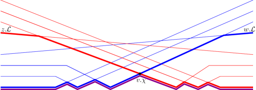
Figure 2: Constructing the lower envelope $v.\mathscr{L}$ (purple) from $w.\mathscr{L}$ (red) and $z.\mathscr{L}$ (blue).

Each node $v$ stores the following variables:

• $f$, $l$, $r$: a pointer to the parent, the left child, and the right child of $v$, respectively; $l,r$ are undefined for a leaf, and $f$ is undefined for the root;

• $\max$: the last pseudo-line in $v.E$ (according to the order defined in Section 2.1);

• $\chi$: the intersection point of $(v.l).\mathscr{L}$ and $(v.r).\mathscr{L}$, the lower envelopes of the left and right children of $v$, if $v$ is an internal node; $\chi$ is undefined for leaves;

• $\Lambda$: a balanced binary search tree (e.g., a red-black tree) that stores the prefix or the suffix of $v.\mathscr{L}$, denoted by $\overline{\mathscr{L}}$, that is not on the lower envelope $(f.v).\mathscr{L}$; the root of $\Xi$ stores the entire envelope $\mathscr{L}(E)$. The leaves of $\Lambda$ represent the segments of $\overline{\mathscr{L}}$ sorted from left to right. Each node $\xi$ of $\Lambda$ is associated with a contiguous portion $\overline{\mathscr{L}}_{\xi}$ of $\overline{\mathscr{L}}$. Each leaf $\xi$ stores the endpoints of $\overline{\mathscr{L}}_{\xi}$, which consists of a single segment, and the pseudo-line of $v.E$ that supports $\overline{\mathscr{L}}_{\xi}$. Each inner node $\xi$ of $\Lambda$, with left and right children $\zeta$ and $\eta$, stores the common endpoint $\xi.p$ of $\overline{\mathscr{L}}_{\zeta}$ and $\overline{\mathscr{L}}_{\eta}$. We note that the two pseudo-lines supporting the last segment of $\overline{\mathscr{L}}_{\zeta}$ and the first segment of $\overline{\mathscr{L}}_{\eta}$ intersect at $\xi.p$ and the lower envelope of these two pseudo-lines, denoted by $\xi.\mathsf{L}$, represents the lower envelope $v.\mathscr{L}$ locally in the neighborhood of $\xi.p$. We store these two pseudo-lines at $\xi$. Since $\xi.\mathsf{L}$ can be computed in $O(1)$ time from the two pseudo-lines, for simplicity, we can assume that we also store $\xi.\mathsf{L}$ at $\xi$. See Section 2.3 below for more details on $\Lambda$.

During our update procedure, we need to perform split and join operations on the secondary trees $v.\Lambda$ at various nodes $v$ in $\Xi$. Each of these procedures can be implemented in $O(\log n)$ time using the standard methods [31, Chapter 4].

Queries.

We now describe the two query operations that we perform on $\Xi$.

Point-location query. Given a value $x_{0}\in\mathbb{R}$, we report the pseudo-line $e\in E$ that contains the point on $\mathscr{L}(E)$ with $x$-coordinate $x_{0}$. Since the root $u$ of $\Xi$ explicitly stores $\mathscr{L}(E)$ in a balanced binary search tree $u.\Lambda$, this query can be answered in $O(\log n)$ time.

Lemma 2.1.

For a given value $x_{0}\in\mathbb{R}$, a point-location query can be answered in $O(\log n)$ time.

Ray-intersection query. Given a point $q\in\mathbb{R}^{2}$, we report all pseudo-lines of $E$ that lie vertically below $q$, i.e., report all pseudo-lines that intersect the ray emanating from $q$ in the $(-y)$-direction.

Let $q_{x}$ be the $x$-coordinate of $q$. We perform a point-location query with $q_{x}$ on $\Xi$ and determine the pseudo-line $e$ that contains the point of $\mathscr{L}(E)$ with $x$-coordinate $q_{x}$. If $q$ lies below $e$, we are done. Otherwise, we store $e$ in the result set and delete $e$ from $\Xi$. We repeat this step until either $\Xi$ becomes empty or $q$ lies below the lower envelope of the remaining set. Finally, we re-insert all elements from the result set to restore the original set of pseudo-lines. Overall, we need $k+1$ point-location queries, $k$ deletions, and $k$ insertions. By Lemma 2.1, each point-location query needs $O(\log n)$ time, and below we show that one update operation requires $O(\log^{2}n)$ time. Hence, we obtain the following.

Lemma 2.2.

Let $q\in\mathbb{R}^{2}$. All $k$ pseudo-lines in $E$ that lie below $q\in\mathbb{R}^{2}$ can be reported in time $O(\log n+k\log^{2}n)$.

Updates.

To insert or delete a pseudo-line $e$ in $\Xi$, we follow the method of Overmars and van Leeuwen [27]. We delete or insert a leaf $z$ for $e$ in $\Xi$ using the standard techniques for balanced binary search trees (the $v.\max$ pointers guide the search in $\Xi$) [31]. We update the secondary structure stored at the nodes of $\Xi$, as follows. Let $\pi$ be the path in $\Xi$ from the root to $z$. As we go down along $\pi$, for each node $v\in\pi$ and its sibling $w$, we construct $v.\mathscr{L}$ and $w.\mathscr{L}$ from $(v.f).\mathscr{L}$, stored as a balanced binary tree. If $v$ is the root, then $v$ already stores $v.\mathscr{L}$, so assume $v$ is not the root and inductively we have $(v.f).\mathscr{L}$ at our disposal. We split $(v.f).\mathscr{L}$ at $(v.f).\chi$, and let $\Lambda^{-}$ (resp. $\Lambda^{+}$) be the prefix (resp. suffix) of $(v.f).\mathscr{L}$. If $v$ is the left child of $v.f$, then $v.\mathscr{L}$ (resp. $w.\mathscr{L}$) is obtained by merging $\Lambda^{-}$ with $v.\Lambda$ ($w.\Lambda$ with $\Lambda^{+}$). If $v$ is the right child, then the roles of $v$ and $w$ are reversed. When we reach the leaf, we have the lower envelope at the siblings of all non-root nodes in $\pi$.

After having inserted or deleted $z$, we trace $\pi$ back in a bottom-up manner. When we reach a node $v$, we have computed $(v.l).\Lambda$, $(v.r).\Lambda$, and $v.\mathscr{L}$. At the node $v$, we first compute the unique intersection point $(v.f).\chi$ of $v.\mathscr{L}$ and $w.\mathscr{L}$, where $w$ is the sibling of $v$, using the procedure described in the next subsection; recall that we already have computed $w.\mathscr{L}$. Suppose $v$ is the left child of its parent. We split $v.\mathscr{L}$ into two parts $\mathscr{L}_{v}^{-},\mathscr{L}_{v}^{+}$ at $(v.f).\chi$, with the former lying to the left. Similarly, we split $w.\mathscr{L}$ into two parts $\mathscr{L}^{-}_{w},\mathscr{L}^{+}_{w}$ at $(v.f).\chi$ (note that $v.f=w.f$) with the former lying to the left. We store $\mathscr{L}_{v}^{+},\mathscr{L}_{w}^{-}$ as $v.\Lambda$ and $w.\Lambda$, respectively. We also update $v.\max$ and $w.\max$. We then merge $\mathscr{L}_{v}^{-}$ and $\mathscr{L}_{w}^{+}$ to obtain $(v.f).\mathscr{L}$. We then move to $v.f$. If we reach the root of $\Xi$, then we simply store the envelope at $v.f$ and stop.

Since the height of $\Xi$ is $O(\log n)$, since each split/merge operations takes $O(\log n)$ time, and since, by Lemma 2.7 below, the intersection point of two envelopes at each node can be computed in $O(\log n)$ time, the update procedure takes $O(\log^{2}n)$ time. More details can be found, e.g., in the original paper by Overmars and van Leeuwen [27] or in the book by Preparata and Shamos [29].

Lemma 2.3.

An insert/delete operation in $\Xi$ takes $O(\log^{2}n)$ time.

2.3 Finding the intersection point of two lower envelopes

Given two lower envelopes $\mathscr{L}_{l}$ and $\mathscr{L}_{r}$, such that all pseudo-lines in $\mathscr{L}_{l}$ are smaller than all pseudo-lines in $\mathscr{L}_{r}$ and each envelope is stored in a balanced binary tree as described above, we give a procedure to compute the (unique) intersection point $q$ between $\mathscr{L}_{l}$ and $\mathscr{L}_{r}$ in $O(\log n)$ time. In our algorithm, $\mathscr{L}_{l}$ and $\mathscr{L}_{r}$ are stored as balanced binary search trees $\Lambda_{l}$ and $\Lambda_{r}$.

The leaves of $\Lambda_{l}$ and $\Lambda_{r}$ represent the segments on the lower envelopes $\mathscr{L}_{l}$ and $\mathscr{L}_{r}$, sorted from left to right. To ensure that every point on $\mathscr{L}_{l}$ and $\mathscr{L}_{r}$ is associated with exactly one leaf of $\Lambda_{l}$ and $\Lambda_{r}$, we use the convention that the segments in the leaves are semi-open, containing their right, but not their left, endpoint in $\Lambda_{l}$ and their left, but not their right, endpoint in $\Lambda_{r}$. Recall that we store both endpoints of a segment as well as the pseudo-line supporting the segment at each leaf of $\Lambda_{l}$ and $\Lambda_{r}$, but the segments are interpreted as relatively semi-open sets, where the precise endpoint to be included depends on the role that the tree plays in the intersection algorithm. More concretely, the intersection algorithm uses two items stored at a leaf $v$ of $\Lambda_{l}$ or $\Lambda_{r}$:

• the pseudo-line $v.\mathscr{L}$ that supports the segment represented by $v$; and

• an endpoint $v.p$ of the segment, namely the left endpoint if $v$ is a leaf of $\Lambda_{l}$, and the right endpoint if $v$ is a leaf of $\Lambda_{r}$. Note that this is exactly the endpoint of the associated segment that is not included in the semi-open segment represented by $v$. This choice is made to ensure a uniform handling of inner nodes and leaves in the intersection algorithm.

Consider an inner node $v$ of $\Lambda_{l}$ or $\Lambda_{r}$. The intersection algorithm uses the two items stored at $v$:

• the lower envelope $v.\mathsf{L}$ of the last (maximum) pseudo-line in the left subtree $v.l$ of $v$ and the first (minimum) pseudo-line in the right subtree $v.r$ of $v$; and

• the intersection point $v.p$ of these two pseudo-lines, which is the only breakpoint of $v.\mathsf{L}$.

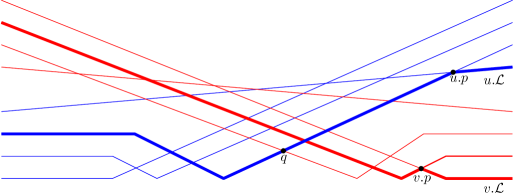
Figure 3: An example of Case 1: The pseudo-lines in $\Lambda_{l}$ are shown blue, the pseudo-lines in $\Lambda_{r}$ are shown red.

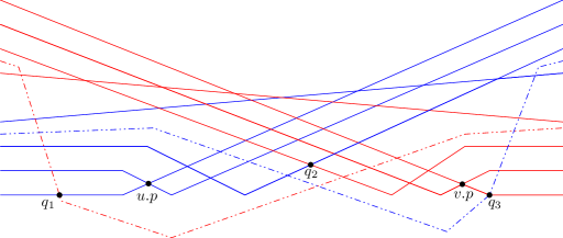
Figure 4: An example of Case 3: The pseudo-lines in $\Lambda_{l}$ (resp. $\Lambda_{r}$) are shown blue (resp. red). The solid pseudo-lines are fixed. The dashed pseudo-lines are optional, meaning that either none or exactly one of the dashed pseudo-lines is present. The current vertices of the binary search are $u.p$ and $v.p$, and Case 3 applies. Irrespective of the local situation at $u$ and $v$, the intersection point $q$ of $\mathscr{L}_{l}$ and $\mathscr{L}_{r}$ might be to the left of $u.p$ (e.g., $q_{1}$ in the figure), between $u.p$ and $v.p$ (e.g., $q_{2}$ in the figure), or to the right of $v.p$ (e.g., $q_{3}$ in the figure), depending on which one of the dashed pseudo-lines is present.

As discussed above, the leaf $u^{*}$ of $\Lambda_{l}$ and the leaf $v^{*}$ of $\Lambda_{r}$ whose (half-open) segments contain the intersection point $q$ between $\mathscr{L}_{l}$ and $\mathscr{L}_{r}$ are uniquely determined. Let $\pi_{l}$ be the path in $\Lambda_{l}$ from the root to $u^{*}$ and $\pi_{r}$ the path in $\Lambda_{r}$ from the root to $v^{*}$. Our strategy is as follows: we simultaneously descend into $\Lambda_{l}$ and $\Lambda_{r}$, following the paths $\pi_{l}$ and $\pi_{r}$, starting from the respective roots. Let $u$ be the current node in $\pi_{l}$ and let $v$ be the current node in $\pi_{r}$. At each step, we perform a local test on $u$ and $v$, comparing $u.p$ with $v.\mathsf{L}$ and $v.p$ with $u.\mathsf{L}$, to decide how to proceed. The test distinguishes among three possibilities:

1. The point $u.p$ lies on or above the (local) lower envelope $v.\mathsf{L}$. In this case, $u.p$ lies on or above the envelope $\mathscr{L}_{r}$. Therefore, the intersection point $q$ between $\mathscr{L}_{l}$ and $\mathscr{L}_{r}$ must be equal to or to the left of $u.p$; see Figure 3. If $u$ is an inner node, then the desired leaf $u^{*}$ cannot lie in the right subtree $u$ (recall that the half-open segments in the leaves of $\Lambda_{l}$ are considered to be open to the left). If $u$ is a leaf, then $u^{*}$ lies strictly to the left of $u$ (recall that in this case, $u.p$ is the left endpoint of the segment stored in $u$, so $u.p$ does not belong to the half-open segment in $u$ but to the half-open segment in the predecessor-leaf).

2. The point $v.p$ lies on or above the (local) lower envelope $u.\mathsf{L}$. In this case, $v.p$ lies on or above the entire envelope $\mathscr{L}_{l}$, therefore the intersection point $q$ between $\mathscr{L}_{l}$ and $\mathscr{L}_{r}$ is equal to or to the right of $v.p$; this situation is symmetric to the one depicted in Figure 3. If $v$ is an inner node, then $v^{*}$ cannot lie in the left subtree $v$ (recall that the segments in the leaves of $\Lambda_{r}$ are considered to be open to the right). If $v$ is a leaf, then $v^{*}$ lies strictly to the right of $v$ (recall that in this case, $v.p$ is the right endpoint of the segment stored in $v$, so $v.p$ does not belong to the half-open segment in $v$, but to the half-open segment in the successor-leaf).

3. The point $u.p$ lies below the (local) lower envelope $v.\mathsf{L}$ and the point $v.p$ lies below the (local) lower envelope $u.\mathsf{L}$: in this case, the point $u.p$ must lie strictly to the left of the point $v.p$. This claim follows from property (B) of pseudo-lines because all pseudo-lines in $\Lambda_{l}$ are smaller than all pseudo-lines in $\Lambda_{r}$; see Figure 4. Thus, it follows that the intersection point $q$ is strictly to the right of $u.p$ or strictly to the left of $v.p$ (both situations can occur simultaneously, if $q$ lies between $u.p$ and $v.p$). In the former case, if $u$ is an inner node, then $u^{*}$ lies in $u.r$ or to the right of all leaves in $u.r$, and if $u$ is a leaf, then either $u^{*}=u$ or $u^{*}$ is a leaf to the right of $u$. In the latter case, if $v$ is an inner node, then $v^{*}$ lies in $v.l$ or to the left of all leaves in $v.l$, and if $v$ is a leaf, then $v^{*}=v$ or $v^{*}$ is a leaf to the left of $v$.

In the first two cases, it is easy to perform the next step in the binary search. In the third case, however, it is not immediately obvious what to do. The correct choice might be either to go to $u.r$ or to $v.l$. For the straight-line case, Overmars and van Leeuwen resolve this ambiguity by comparing the slopes of the relevant lines. For pseudo-lines, however, there is no notion of slope. Even worse, it seems that there is no local test to resolve this situation. For an example, refer to Figure 4, where the local situation at $u$ and $v$ does not help to determine the position of the intersection point $q$. We present an alternative strategy, which also applies for pseudo-lines.

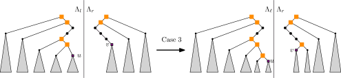
Figure 5: Comparing $u$ to $v$: in Case 3, we know that $u^{*}$ is in $u.r$ or $v^{*}$ is in $v.l$; we go to $u.r$ and to $v.\ell$.

Throughout the search, we maintain the invariant that the subtree at the current node $u$ of $\Lambda_{l}$ contains the desired leaf $u^{*}$ or the subtree at the current node $v$ of $\Lambda_{r}$ contains the desired node $v^{*}$ (or both). In Case 3, as explained above, it holds that $u^{*}$ must be in $u.r$ or $v^{*}$ must be in $v.l$ (or both); see Figure 5. Thus, we will move $u$ to $u.r$ and $v$ to $v.l$. One of these moves must be correct, but the other move might be mistaken: we might go to $u.r$ even though $u^{*}$ is in $u.l$; or to $v.l$ even though $v^{*}$ is in $v.r$. To account for this possible mistake, we remember the current node $u$ in a stack uStack and the current node $v$ in a stack vStack. Then, if it becomes necessary, we can backtrack and revisit the other subtree $u.l$ or $v.r$. This approach leads to the general situation shown in Figure 6: The desired leaf $u^{*}$ is in the subtree of $u$ or in a left subtree of a node on uStack, while the desired leaf $v^{*}$ is in the subtree of $v$ or in a right subtree of a node on vStack, and at least one of $u^{*}$ or $v^{*}$ must be in the subtree of $u$ or of $v$, respectively. Now, if Case 1 occurs when comparing $u$ to $v$, we can exclude the possibility that $u^{*}$ is in $u.r$. Thus, $u^{*}$ might be in $u.l$, or in the left subtree of a node in uStack; see Figure 7. To make progress, we now compare $u^{\prime}$, the top of uStack, with $v$. Again, one of the three cases occurs:

• In Case 1, we can deduce that going to $u^{\prime}.r$ was mistaken, and we move $u$ to $u^{\prime}.l$, while $v$ does not move.

• In the other cases, we cannot rule out that $u^{*}$ is to the right of $u^{\prime}$, and we move $u$ to $u.l$, keeping the invariant that $u^{*}$ is either below $u$ or in the left subtree of a node on uStack. However, to ensure that the search progresses, we now must also move $v$:

  • In Case 2, we can rule out that $v^{*}$ lies in $v.l$, and we move $v$ to $v.r$.

  • In Case 3, we move $v$ to $v.l$.

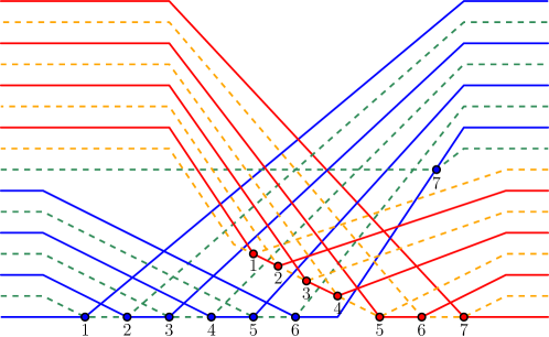
Figure 18: Two sets of pseudo-lines and their lower envelopes: (i) the blue and green pseudo-lines, (ii) the red and orange pseudo-lines. The blue and the red dots represent the vertices on the lower envelopes.

In this way, we keep the invariant and always make progress: in each step, we either discover at least one new node on either of the two correct search paths, or we pop one erroneous move from one of the two stacks. Since the total length of the correct search paths is $O(\log n)$, and since we push a new element onto the stack only when discovering a new node on either of the correct search paths, the total search time is $O(\log n)$; see Figures 18 and 19 and Table 1 in Appendix for an example run of the algorithm.

The following pseudo-code gives the details of our algorithm, including all corner cases.

oneStep($u$, $v$)

do compare($u$, $v$):

Case 3:

if $u$ is not a leaf then

      uStack.push($u$); $u\leftarrow u.r$

      end if

     if $v$ is not a leaf then

           vStack.push($v$); $v\leftarrow v.l$

           end if

          if $u$ and $v$ are leaves then

                return $u=u^{*}$ and $v=v^{*}$

                end if

               Case 1:

                if uStack is empty then

                     $u\leftarrow u.l$;

                    

                     else if  $u$ is a leaf then

                          $u\leftarrow\texttt{uStack.pop().}l$

                          else

                               $u^{\prime}\leftarrow\texttt{uStack.top()}$

                               do compare($u^{\prime}$, $v$)

                               Case 1:

                               uStack.pop(); $u\leftarrow u^{\prime}.l$;

                               Case 2:

                               $u\leftarrow u.l$

                               if $v$ is not a leaf then

                                    $v.\leftarrow v.r$

                                    end if

                                   Case 3:

                                    $u\leftarrow u.l$

                                    if  $v$ is not a leaf then

                                         vStack.push($v$); $v\;\leftarrow v.l$

                                         end if

                                        

                                         end if

                                        Case 2:

symmetric

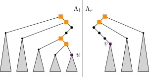
Figure 6: The invariant: the current search nodes are $u$ and $v$. uStack contains all nodes on the path from the root to $u$ where the path goes to a right child (orange squares), vStack contains all nodes from the root to $v$ where the path goes to a left child (orange squares). The final leaves $u^{*}$ and $v^{*}$ are in one of the gray subtrees; and at least one of them is under $u$ or under $v$.

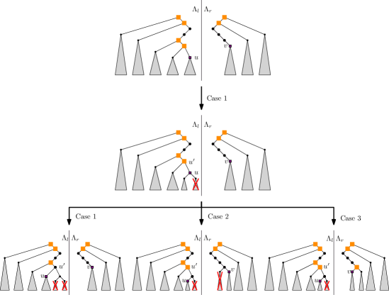
Figure 7: Comparing $u$ to $v$: in Case 1, we know that $u^{*}$ cannot be in $u.r$. We compare $u^{\prime}$ and $v$ to decide how to proceed: in Case 1, we know that $u^{*}$ cannot be in $u^{\prime}.r$; we go to $u^{\prime}.l$; in Case 2, we know that $u^{*}$ cannot be in $u.r$ and that $v^{*}$ cannot be in $v.l$; we go to $u.l$ and to $v.r$; in Case 3, we know that $u^{*}$ is in $u^{\prime}.r$ (and hence in $u.l$) or in $v.l$; we go to $u.l$ and to $v.l$. Case 2 is not shown, as it is symmetric.

We will show that the search procedure maintains the following invariant:

Invariant 2.4.

The leaves in all subtrees $u^{\prime}.l$, for $u^{\prime}\in\textup{{uStack}}$, together with the leaves under $u$ constitute a prefix of the leaves in $\Lambda_{l}$. This prefix contains $u^{*}$. Similarly, the leaves in all subtrees $v^{\prime}.r$, $v^{\prime}\in\textup{{vStack}}$, together with the leaves under $v$ constitute a contiguous suffix of the leaves of $\Lambda_{r}$. This suffix contains $v^{*}$. Furthermore, we have $u\in\pi_{l}$ or $v\in\pi_{r}$ (or both).

Invariant 2.4 holds at the beginning, when both stacks are empty, $u$ is the root of $\Lambda_{l}$ and $v$ is the root of $\Lambda_{r}$. To show that the invariant is maintained, we first consider the special case when one of the two searches has already discovered the correct leaf. Recall that $\pi_{l},\pi_{r}$ are the root-to-leaf paths to $u^{*}$, $v^{*}$ in $\Lambda_{l}$ and $\Lambda_{r}$, respectively.

Lemma 2.5.

Suppose that Invariant 2.4 holds and that Case 3 occurs when comparing $u$ to $v$. If $u=u^{*}$, then $v\in\pi_{r}$ and, if $v$ is not a leaf, then $v.l\in\pi_{r}$. Similarly, if $v=v^{*}$, then $u\in\pi_{l}$ and, if $u$ is not a leaf, then $u.r\in\pi_{l}$.

Proof.

We consider the case $u=u^{*}$; the other case is symmetric. Let $e_{u}$ be the segment of $\mathscr{L}_{l}$ stored in $u$. By Case 3, the point $u.p$ is strictly to the left of the point $v.p$. Furthermore, since $u=u^{*}$, the intersection point $q$ lies on $e_{u}$. Thus, $q$ cannot be to the right of $v.p$, because otherwise $v.p$ would be a point on $\mathscr{L}_{r}$ that lies below $e_{u}$ and to the left of $q$, which is impossible. Since $q$ is strictly to the left of $v.p$, Invariant 2.4 shows that if $v$ is an inner node, then $v^{*}$ must be in $v.l$ (and hence both $v$ and $v.l$ lie on $\pi_{r}$), and if $v$ is a leaf, then $v=v^{*}$. ∎

We can now show that the invariant is maintained.

Lemma 2.6.

Procedure oneStep either correctly reports the desired leaves $u^{*}$ and $v^{*}$, or maintains Invariant 2.4. In the latter case, either it pops an element from one of the two stacks, or it discovers a new node on $\pi_{\ell}$ or $\pi_{r}$.

Proof.

First, suppose Case 3 occurs. The invariant that uStack and $u$ cover a prefix of $\mathscr{L}_{l}$ and that vStack and $v$ cover a suffix of $\mathscr{L}_{r}$ is maintained. Furthermore, if both $u$ and $v$ are inner nodes, Case 3 ensures that $u^{*}$ is in $u.r$ or to the right of $u$, or that $v^{*}$ is in $v.l$ or to the left of $v$. Suppose the former case holds. Then, Invariant 2.4 implies that $u^{*}$ must be in $u.r$, and hence $u$ and $u.r$ lie on $\pi_{l}$. Similarly, in the second case, Invariant 2.4 gives that $v$ and $v.l$ lie on $\pi_{r}$. Thus, Invariant 2.4 is maintained and we discover a new node on $\pi_{l}$ or on $\pi_{r}$. Now, assume $u$ is a leaf and $v$ is an inner node. If $u\neq u^{*}$, then as above, Invariant 2.4 and Case 3 imply that $v\in\pi_{r}$ and $v.l\in\pi_{r}$, and the lemma holds. If $u=u^{*}$, the lemma follows from Lemma 2.5. The case that $u$ is an inner node and $v$ a leaf is symmetric. If both $u$ and $v$ are leaves, Lemma 2.5 implies that oneStep correctly reports $u^{*}$ and $v^{*}$.

Second, suppose Case 1 occurs. Then, $u^{*}$ cannot be in $u.r$, if $u$ is an inner node, or $u^{*}$ must be to the left of a segment left of $u$, if $u$ is a leaf. Now, if uStack is empty, Invariant 2.4 and Case 1 imply that $u$ cannot be a leaf (because $u^{*}$ must be in the subtree of $u$) and that $u.l$ is a new node on $\pi_{l}$. Thus, the lemma holds in this case. Next, if $u$ is a leaf, Invariant 2.4 and Case 1 imply that $v\in\pi_{r}$. Thus, we pop uStack and maintain the invariant; the lemma holds. Now, assume that uStack is not empty and that $u$ is not a leaf. Let $u^{\prime}$ be the top of uStack. First, if the comparison between $u^{\prime}$ and $v$ results in Case 1, then $u^{*}$ cannot be in $u^{\prime}.r$, and in particular, $u\not\in\pi_{l}$. Invariant 2.4 shows that $v\in\pi_{r}$, and we pop an element from uStack, so the lemma holds. Second, if the comparison between $u^{\prime}$ and $v$ results in Case 2, then $v^{*}$ cannot be in $v.l$, if $v$ is an inner node. Also, if $u\in\pi_{l}$, then necessarily also $u.l\in\pi_{l}$, since Case 1 occurred between $u$ and $v$. If $v\in\pi_{r}$, since Case 2 occurred between $u^{\prime}$ and $v$, the node $v$ cannot be a leaf and $v.r\in\pi_{r}$. Thus, in either case the invariant is maintained and we discover a new node on $\pi_{l}$ or on $\pi_{r}$. Third, assume the comparison between $u^{\prime}$ and $v$ results in Case 3. If $u\in\pi_{l}$, then also $u.l\in\pi_{l}$, because $u.r\in\pi_{l}$ was excluded by the comparison between $u$ and $v$. In this case, the lemma holds. If $u\not\in\pi_{l}$, then also $u^{\prime}.r\not\in\pi_{l}$, so the fact that Case 3 occurred between $u^{\prime}$ and $v$ implies that $v.l$ must be on $\pi_{r}$ (in this case, $v$ cannot be a leaf, since otherwise we would have $v^{*}=v$ and Lemma 2.5 would give $u^{\prime}.r\in\pi_{l}$, which we have already ruled out). The argument for Case 2 is symmetric. ∎

The following lemma finally shows that our intersection procedure finds the desired point in logarithmic time.

Lemma 2.7.

The intersection point $q$ between $\mathscr{L}_{l}$ and $\mathscr{L}_{r}$ can be computed in $O(\log n)$ time.

Proof.

In each step, we either discover a new node of $\pi_{l}$ or of $\pi_{r}$, or we pop an element from uStack or vStack. Elements are pushed only when at least one new node on $\pi_{l}$ or $\pi_{r}$ is discovered. As $\pi_{l}$ and $\pi_{r}$ are each a path from the root to a leaf in a balanced binary tree, we need $O(\log n)$ steps. ∎

Putting everything together, we obtain the following:

Theorem 2.8.

A set $E$ of $n$ pseudo-lines can be maintained in a data structure so that (i) a pseudo-line can be inserted/deleted in $O(\log^{2}n)$ time; (ii) for a query value $x_{0}\in\mathbb{R}$, the point of $\mathscr{L}(E)$ with the $x$-coordinate $x_{0}$ and the input pseudo-line containing this point can be computed in $O(\log n)$ time; and (iii) all $k$ pseudo-lines of $E$ lying below a query point $q\in\mathbb{R}^{2}$ can be reported in $O(\log n+k\log^{2}n)$ time.

3 Maintaining the Union of Unit Discs under Insertions

Let $S$ be a set of $n$ points in $\mathbb{R}^{2}$, and let $U:=U(S)=\bigcup_{p\in S}D(p)$ be the union of the unit discs centered at the points of $S$. In this section, we describe a data structure that maintains $\mathscr{E}$, the set of edges of $\partial U$. After the insertion of a new point to $S$, it updates $\mathscr{E}$ in $O(\log n+k\log^{2}n)$ time, where $k$ is the number of changes (insertions plus deletions) in the set $\mathscr{E}$. It can also report, within the same time bound, the area of $U$, denoted $\mathop{\mathrm{Area}}U$, after the insertion of each point.

This section is organized as follows. Section 3.1 gives a high-level description of the overall data structure and of the update procedure. Section 3.2 describes the data structure for reporting the set of edges in $\mathscr{E}$ that intersect a unit disc, which relies on the data structure described in the previous section. Finally, Section 3.3 proves a few key properties of $\mathscr{E}$ that are crucial for our data structure.

3.1 Overview of the data structure

The overall data structure consists of two parts. Let $\mathbb{G}$ be a uniform grid in $\mathbb{R}^{2}$ such that the diameter of each grid cell is $1$. We call a grid cell of $\mathbb{G}$ active if it intersects $U$. Let $\mathscr{G}\subset\mathbb{G}$ be the set of active grid cells. Each unit disc intersects $O(1)$ grid cells, so $|\mathscr{G}|=O(n)$. We define the key of a grid cell to be the $x$- and $y$-coordinates of its bottom left corner, and we induce a total ordering on the grid cells by using the lexicographic ordering on their keys. Using this total ordering, we store $\mathscr{G}$ in a balanced binary search tree (e.g. red-black tree) $\Omega$. A membership query and an update operation on $\mathscr{G}$ can be performed in $O(\log n)$ time [31].

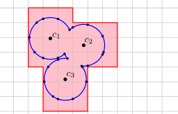
Figure 8: The grid imposed over the union of unit discs. The active cells are highlighted in pale red.

We overlay $U$ with $\mathbb{G}$. If an edge of $\partial U$ intersects more than one grid cell, then we split it at the boundaries of the cells that it crosses (see Figure 8). We can therefore assume that each edge of $\mathscr{E}$ lies within a single cell. For each cell $C\in\mathscr{G}$, let $\mathscr{E}_{C}\subseteq\mathscr{E}$ denote the set of edges that lie inside $C$. We maintain $\mathscr{E}_{C}$ in a dynamic data structure $\Psi_{C}$, described in Section 3.2, that

• for a query point $q$, reports, in $O(\log n+k_{C}\log^{2}n)$ time, the subset $\mathscr{E}_{q,C}\subseteq\mathscr{E}_{C}$ of edges that intersect $D(q)$, where $k_{C}=|\mathscr{E}_{q,C}|$; and

• can handle insertion or deletion of an edge in $\mathscr{E}_{C}$ in $O(\log^{2}n)$ time.

See Lemma 3.7 below.

Using $\Omega$ and $\Psi_{C}$, for all grid cells $C\in\mathscr{G}$, the insertion of a point $q$ into $S$ is handled as follows. To avoid confusion, we use $U$ (resp. $U^{\mathrm{new}}$) to denote $U(S)$ immediately before (resp. after) the insertion of $q$.

1. Compute the set $\mathbb{G}_{q}$ of $O(1)$ grid cells that the new disc $D(q)$ intersects.

2. Find the subset $\mathscr{G}_{q}=\mathbb{G}_{q}\cap\mathscr{G}$ of active cells (before the insertion of $q$) that intersect $D(q)$.

3. For each cell $C\in\mathscr{G}_{q}$, using the data structure $\Psi_{C}$, report the subset $\mathscr{E}_{q,C}\subseteq\mathscr{E}_{C}$ of edges that $D(q)$ intersects. Set $\mathscr{E}_{q}=\bigcup_{C\in\mathscr{G}_{q}}\mathscr{E}_{q,C}$ and $k=|\mathscr{E}_{q}|$.

4. Compute the set $I_{q}$ of new edges on $U^{\mathrm{new}}$. We split the edges of $I_{q}$ at the grid boundaries so that each edge lies within one grid cell. For each cell $C\in\mathbb{G}_{q}$, let $I_{q,C}\subseteq I_{q}$ be the set of edges that lie inside $C$.

5. For each cell $C\in\mathbb{G}_{q}$, delete the edges of $\mathscr{E}_{q,C}$ from $\Psi_{C}$ and insert the edges of $I_{q,C}$ into $\Psi_{C}$. If $C\not\in\mathscr{G}$, insert $C$ into $\Omega$.

6. Compute $\mathop{\mathrm{Area}}U^{\mathrm{new}}$.

Steps 1 and 2 are straightforward and can be implemented in $O(\log n)$ time using $\Omega$. Steps 3 and 5 can be implemented using the procedures described in Section 3.2. By Lemma 3.7, the total time spent in these two steps is $O(\log n+(k+|I_{q}|)\log^{2}n)=O((k+1)\log^{2}n)$ because as we will see below, $|I_{q}|=O(k+1)$. We now describe how to compute the set $I_{q}$ of new edges (Step 4) and $\mathop{\mathrm{Area}}U^{\mathrm{new}}$ (Step 6).

Updating the boundary of the union.

First, consider the case when $k=0$, then either $D(q)\subset U$ or $D(q)\cap U=\emptyset$. Since the diameter of each grid cell in $\mathbb{G}$ is $1$, at least one of the grid cells, denoted by $\omega$, is fully contained in $D(q)$. If $\omega\in\mathscr{G}_{q}$, then $\omega\subset U$ (because $\omega\cap U\neq\emptyset$ but $\omega\cap\partial U=\emptyset$ since $\mathscr{E}_{q}=\emptyset$) and therefore $D(q)\subset U$; otherwise $D(q)\cap U=\emptyset$. If $D(q)\subset U$, then $\partial U^{\mathrm{new}}=\partial U$, and there is nothing to do. On the other hand, if $D(q)\cap U=\emptyset$, then the entire $\partial D(q)$ appears on $\partial U^{\mathrm{new}}$. We split $\partial D(q)$ at the boundary of the grid cells, and $I_{q}$ is the resulting set of edges.

We now assume that $k>0$. The set $I_{q}$ contains two types of edges:

• The edges that lie on the boundaries of older discs. These edges are the portions of the edges of $\mathscr{E}_{q}$ that lie outside $D(q)$.

• The edges that lie on $\partial D(q)$. These edges are (maximal) connected arcs of $\partial D(q)\setminus U$.

To compute the first type of edges, for each edge $e\in\mathscr{E}_{q}$, we compute the intersection points of $e\cap\partial D(q)$. If $e\not\subset D(q)$ then we compute $e\setminus D(q)$, which comprises one or two arcs, and which we add to $I_{q}$.

Let $V$ be the set of intersection points of $\partial D(q)$ and the edges of $\mathscr{E}_{q}$. We sort $V$ along $\partial D(q)$. These intersection points partition $\partial D(q)$ into arcs. Each such arc $\gamma$ either lies inside $U$ or outside $U$, and we can detect it in $O(1)$ time. If $\gamma$ lies outside $U$, we add $\gamma$ to $I_{q}$.

It follows from the above discussion that $|I_{q}|=O(k+1)$ and that the total time spent in computing $I(q)$ is $O((k+1)\log n)$.

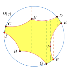
Figure 9: Arrangement $\mathscr{A}$ and its vertical decomposition $\mathscr{A}^{\nabla}$; shaded pseudo-trapezoids do not lie in $U$.

Computing the area of the union.

We now describe how we extend the procedure for computing $I_{q}$ to compute $\Delta A=\mathop{\mathrm{Area}}U^{\mathrm{new}}-\mathop{\mathrm{Area}}U$. If $k=0$, then as described above, we determine whether $D(q)\subset U$ or $D(q)\cap U=\emptyset$. We have $\Delta A=0$ in the former case, and $\Delta A=\mathop{\mathrm{Area}}D(q)=\pi$ in the latter case. We now focus on the case $k>0$.

Let $\mathscr{E}_{q}^{\mathrm{in}}=\{e\cap D(q)\mid e\in\mathscr{E}_{q}\}$ be the portions of edges in $\mathscr{E}_{q}$ clipped within $D(q)$. $\mathscr{E}_{q}^{\mathrm{in}}$ can be computed, in $O(k)$ time, by adapting the procedure for computing $I_{q}$. We note that the relative interiors of edges in $\mathscr{E}_{q}^{\mathrm{in}}$ are pairwise disjoint. Let $\mathscr{A}$ be the arrangement of $\mathscr{E}_{q}^{\mathrm{in}}\cup\partial D(q)$ within $D(q)$, i.e., the decomposition of $D(q)$ induced by these arcs (see [20] for further details on geometric arrangements). Let $\mathscr{A}^{\nabla}$ be the vertical decomposition of $\mathscr{A}$, i.e., the refinement of $\mathscr{A}$ obtained by drawing vertical rays in both $+y$- and $-y$-directions from each vertex of $\mathscr{A}$ or a point of vertical tangency on an arc of $\mathscr{E}_{q}^{\mathrm{in}}$, within $D(q)$, until it meets another edge of $\mathscr{A}$. $\mathscr{A}^{\nabla}$ partitions the faces of $\mathscr{A}$ into pseudo-trapezoids, each bounded by at most two vertical segments and by two circular arcs at top and bottom. See Figure 9. Each pseudo-trapezoid $\tau\in\mathscr{A}^{\nabla}$ is either contained in $U$ or disjoint from $U$. Let $\mathscr{F}$ be the set of faces of $\mathscr{A}^{\nabla}$ that do not lie in $U$. Then $\Delta A=\sum_{\tau\in\mathscr{F}}\mathop{\mathrm{Area}}\tau$.

$\mathscr{A}^{\nabla}$ can be computed in $O(k\log k)$ time using a sweep-line algorithm [10] (recall that $k>0$ here). The sweep-line algorithm can be adapted in a straight-forward manner to compute $\mathscr{F}$ within the same time bound. For each face $\tau\in\mathscr{F}$, we compute $\mathop{\mathrm{Area}}\tau$ in $O(1)$ time and then add them up to compute $\Delta A$. Finally, we set $\mathop{\mathrm{Area}}U^{\mathrm{new}}=\mathop{\mathrm{Area}}U+\Delta A$. After having computed the edges of $U^{\mathrm{new}}$, the total time spent in computing $\mathop{\mathrm{Area}}U^{\mathrm{new}}$ is $O(k\log k)$.

Putting everything together, we obtain the following.

Theorem 3.1.

(i) The boundary edges of the union of a set of $n$ unit discs can be maintained under insertion in a data structure of $O(n)$ size so that a new disc can be inserted in $O((k+1)\log^{2}n)$ time, where $k$ is the total number of changes on the boundary of the union.

(ii) The same data structure can also report the area of the union after the insertion of each disc in $O((k+1)\log^{2}n)$ time, where $k$, as above, is the total number of changes on the boundary of the union.

3.2 Edge intersection data structure

Let $C$ be an axis-parallel square with diameter $1$, representing a grid cell of $\mathbb{G}$, and let $\mathscr{E}_{C}$ be the set of edges of $\partial U$ that lie in $C$. We describe a dynamic data structure $\Psi_{C}$ to report the edges of $\mathscr{E}_{C}$ intersected by a unit disc. It can quickly insert or delete an edge of $\mathscr{E}_{C}$.

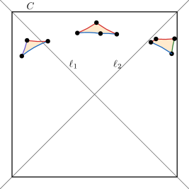
Figure 10: An example of $\partial U\cap C$ with four types of edges $E_{t}$ (red), $E_{b}$ (blue), $E_{l}$ (magenta), and $E_{r}$ (green).

Let $\ell_{1}$ and $\ell_{2}$ be the lines that support the diagonals of $C$. The lines $\ell_{1}$ and $\ell_{2}$ divide the plane into four quadrants: the top quadrant $Q_{t}$, the right quadrant $Q_{r}$, the bottom quadrant $Q_{b}$, and the left quadrant $Q_{l}$. We partition the edges of $\mathscr{E}_{C}$ into four sets $E_{t}$, $E_{r}$, $E_{b}$, and $E_{l}$, depending on which quadrant $Q_{t}$, $Q_{r}$, $Q_{b}$, or $Q_{l}$ contains the center of the respective disc; see Figure 10. If a disc center lies on a dividing line $\ell_{1}$, $\ell_{2}$, then the tie is broken in favor of $E_{t}$ or of $E_{b}$ (in that order). We focus on the edges of $E_{t}$; analogous statements hold also for the other three edge sets. Before describing the data structure, we prove a few key properties of $E_{t}$.

Lemma 3.2.

Each edge in $E_{t}$ is a portion of a lower semi-circle.

Proof.

Let $e\in E_{t}$, and let $c\in Q_{t}$ be the center of the unit disc whose boundary contains $e$. Since the cell $C$ has unit diameter, $c$ lies outside $C$ and above the line that supports the top side of $C$. Thus, $e$, which lies inside $C$, is a portion of the open lower semi-circle of $D(c)$. ∎

Lemma 3.3.

The $x$-projections of the (relative interiors of the) edges in $E_{t}$ are pairwise disjoint.

Proof.

Let $e_{i}$ and $e_{j}$ be two distinct edges of $E_{t}$. Suppose that there is a vertical line $\ell$ that intersects both $e_{i}$ and $e_{j}$, in points $p_{i}$ and $p_{j}$, respectively. For concreteness, assume that $p_{i}$ lies below $p_{j}$. By Lemma 3.2, the point $p_{i}$ lies on the lower semi-circle of a disc $D_{i}$ whose center is above the upper side of $C$. This means that the vertical segment that connects $p_{i}$ to the upper side of $C$ is fully contained in $D_{i}$. But then, $p_{j}$ cannot be on the boundary $\partial U$ of $U$. Thus, the vertical line $\ell$ cannot exist, and the $x$-projections of the edges in $E_{t}$ have pairwise disjoint interiors. ∎

By Lemma 3.3, the edges in $E_{t}$ can be ordered from left to right, according to their $x$-projections. We number them as $e_{1},\dots,e_{m}$, according to this order.

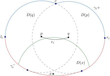
Figure 11: An arc $e_{i}$ of $E_{t}$ with endpoints $p$ and $q$, its Minkowski sum with a unit disc, and its upper (blue) and lower arcs (red) $\gamma^{+}$ and $\gamma^{-}$ respectively. A unit disc $D(q)$ intersects $e_{i}$ if and only if $q$ lies above $\gamma_{i}^{-}$ and below $\gamma_{i}^{+}$.

For an edge $e_{i}\in E_{t}$, let $K_{i}=e_{i}\oplus D(0)$ be the Minkowski sum of $e_{i}$ with the unit disc centered at the origin, i.e.,

$$K_{i}=\{a\in\mathbb{R}^{2}\mid\exists b\in e_{i}\,\|a-b\|\leq 1\}.$$

It is easily seen that a unit disc $D(q)$ intersects $e_{i}$ if and only if $q\in K_{i}$. See Figure 11. We divide $\partial K_{i}$ at its leftmost and rightmost points $l_{i},r_{i}$ into an upper arc $\gamma_{i}^{+}$ and a lower arc $\gamma_{i}^{-}$. We say that a point $x$ lies above (resp. below) an arc if the vertical ray emanating from $x$ in $+y$-direction (resp. $-y$-direction) intersects the arc. The following observation is straightforward:

Lemma 3.4.

• The unit disc $D(q)$ intersects $e_{i}$ if and only if $q$ lies below $\gamma_{i}^{+}$ and above $\gamma_{i}^{-}$.

• Let $c$ be the center of the unit disc whose boundary contains $e_{i}$, and let $p$ and $q$ be the endpoints of $e_{i}$. The upper arc $\gamma_{i}^{+}$ is the upper envelope of the upper semi-circles of $D(p)$ and $D(q)$. The lower arc $\gamma_{i}^{-}$ consists of portions of the lower semi-circles of $D(p)$, $D(q)$, and the disc of radius $2$ centered at $c$.

Set $\Gamma^{+}=\{\gamma_{i}^{+}\mid e_{i}\in E_{t}\}$ and $\Gamma^{-}=\{\gamma_{i}^{-}\mid e_{i}\in E_{t}\}$. The following lemma states three crucial properties of the arcs in $\Gamma^{+}$ and $\Gamma^{-}$.

Lemma 3.5.

The arcs in $\Gamma^{+}$ and $\Gamma^{-}$ have the following properties.

(P1)

Let $e_{i},e_{j}\in E_{t}$ be two distinct edges with $i<j$. Then the lower arcs $\gamma_{i}^{-}$ and $\gamma_{j}^{-}$ intersect and cross in exactly one point, and $\gamma_{i}$ (resp. $\gamma_{j}$) appears on $\mathscr{L}(\{\gamma_{i}^{-},\gamma_{j}^{-}\})$ only before (resp. after) their intersection point.

(P2)

Let $e_{i}$, $e_{j}$, and $e_{h}$ be three edges in $E_{t}$ with $i<j<h$, and let $q\in\mathbb{R}^{2}$. If $q$ lies below $\gamma_{i}^{+}$ and $\gamma^{+}_{h}$, then $q$ also lies below $\gamma^{+}_{j}$. Furthermore, the upper semi-circle of the disc centered at every endpoint of an edge in $E_{t}$ appears on the upper envelope $\mathscr{U}(\Gamma^{+})$, and the order of arcs on $\mathscr{U}(\Gamma^{+})$ corresponds to the $x$-order of the endpoints of the edges of $E_{t}$.

(P3)

For every vertical line $\ell$, all intersection points of $\ell$ with the arcs in $\Gamma^{-}$ lie below all intersection points of $\ell$ with the arcs in $\Gamma^{+}$.

Lemma 3.5 is proved in Section 3.3. In the remainder of this section, we describe the edge-intersection data structure and the query procedure assuming Lemma 3.5 holds.

The data structure $\Psi_{C}$ for $E_{t}$ consists of two parts: $\Delta^{+}$ and $\Delta^{-}$ that dynamically maintain the sets $\Gamma^{+}$ and $\Gamma^{-}$, respectively. The purpose of $\Delta^{+}$ (resp. $\Delta^{-}$) is to efficiently answer the following query: given a point $q\in\mathbb{R}^{2}$, report the upper (resp. lower) arcs that are above (resp. below) $q$. Additionally, $\Delta^{+}$ has the property that it returns the answer incrementally, one arc at a time on demand. Both $\Delta^{+},\Delta^{-}$ support insertion/deletion of arcs.

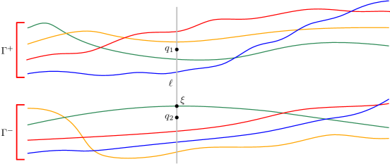
Figure 12: Illustration of the search procedure. There are four pairs of upper and lower arcs (each pair has a distinct color), and two query points $q_{1}$ and $q_{2}$ lying on a vertical line $\ell$; $\xi$ is the intersection point of $\ell$ with $\mathscr{U}(\Gamma^{-})$. The point $q_{1}$ (resp. $q_{2}$) lies above (resp. below) $\xi$, so it suffices to search in $\Gamma^{+}$ (resp. $\Gamma^{-}$).

Answering an edge-intersection query.

With $\Delta^{+},\Delta^{-}$ at our disposal, the edges of $E_{t}$ that intersect a unit disc $D(q)$ are reported as follows. By Lemma 3.4 (i), we wish to report the edges $e_{i}$ such that $\gamma_{i}^{-}$ lies below $q$ and $\gamma_{i}^{+}$ lies above $q$. Here is the basic idea: Let $\ell$ be the vertical line passing through $q$. Assume, for the sake of exposition, that we know the intersection point $\xi$ between $\ell$ and the upper envelope of $\Gamma^{-}$. If $q$ lies above $\xi$ (e.g., $q_{1}$ in Figure 12), then $q$ lies above all the lower arcs that cross $\ell$. Therefore it suffices to search the structure $\Delta^{+}$ to report the upper arcs $\gamma_{i}^{+}$ that lie above $q$—in this case, $e_{i}$ intersects $D(q)$ if and only if $\gamma_{i}^{+}$ lies above $q$. On the other hand, if the center $q$ coincides with or lies below $\xi$ (e.g., $q_{2}$ in Figure 12), then by property (P3), $q$ lies below all upper arcs that $\ell$ intersects. We therefore search $\Delta^{-}$ to report the lower arcs that lie below $q$—in this case, $e_{i}$ intersects $D(q)$ if and only if $\gamma_{i}^{-}$ lies below $q$.

Unfortunately, we cannot easily maintain $\mathscr{U}(\Gamma^{-})$ and thus cannot compute the point $\xi$. Hence, the query procedure is a bit more involved: We use $\Delta^{+}$ to return the upper arcs that lie above $q$ incrementally, one by one, on demand. For each upper arc $\gamma_{i}^{+}$ reported by $\Delta^{+}$, we check in $O(1)$ time whether $e_{i}$ intersects $D(q)$. If so, we add $e_{i}$ to the output list and ask $\Delta^{+}$ to report the next upper arc that lies above $q$. If all the upper arcs above $q$ turn out to be induced by edges of $E_{t}$ that intersect $D(q)$, we output this list of edges as the desired set $\mathscr{E}_{q}$ and stop. Indeed, if all the reported edges from the query of $\Delta^{+}$ intersect $D(q)$, then we can conclude that $q$ is above $\xi$ and this is the complete answer.

On the other hand, if we detect that the edge $e_{j}\in E_{t}$ corresponding to an upper arc $\gamma_{j}^{+}$ reported by $\Delta^{+}$ does not intersect $D(q)$, then by Lemma 3.4 (i), $q$ lies below $\gamma_{i}^{-}$ and thus below $\xi$. As argued above, in this case, we will obtain the full result by querying $\Delta^{-}$. We note that an edge of $E_{t}$ intersecting $D(q)$ is reported at most twice.

As we will see below, if $|\mathscr{E}_{q}|=k$ then searching in $\Delta^{-},\Delta^{+}$ takes $O(\log n+k\log^{2}n)$ and $O(\log n+k)$ time, respectively. Hence, the total query time is $O(\log n+k\log^{2}n)$. We now describe the data structures $\Delta^{-}$ and $\Delta^{+}$.

Maintaining the lower arcs.

We extend each lower arc $\gamma_{i}^{-}$ into a bi-infinite curve $\overline{\gamma}_{i}^{-}$ by adding a ray of very large positive (resp. negative) slope in the $+y$-direction from its right (resp. left) endpoint; see Figure 13. We choose the same slope for all rays and their values are chosen infinitely large so that any query point $q$ lies below the extended curve if and only if it lies below the original lower arc $\gamma_{i}^{-}$. (We should regard this extension as symbolic in the sense that we do not choose any specific value of the slope of these rays.) Let $\overline{\Gamma}^{-}$ denote the resulting set of bi-infinite curves.

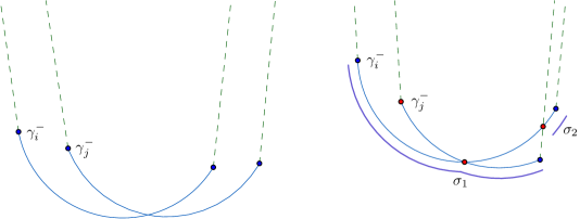
Figure 13: (a) Extending each lower arc to a bi-infinite curve. (b) Illustration of the proof of Lemma 3.6.

Lemma 3.6.

$\overline{\Gamma}^{-}$ is a set of pseudo-lines. Furthermore, $\mathscr{L}(\overline{\Gamma}^{-})$ is the same as $\mathscr{L}(\Gamma^{-})$ except the two extension rays that appear as unbounded segments at each end of the lower envelope.

Proof.

Suppose there are two extended curves $\overline{\gamma}_{i}^{-},\overline{\gamma}_{j}^{-}\in\overline{\Gamma}^{-}$, with $i<j$, that intersect at two points $\sigma_{1},\sigma_{2}$. By (P1), one of these intersection points, say, $\sigma_{1}$, is the intersection point of $\gamma_{i}^{-}$ and $\gamma_{j}^{-}$, and $\gamma_{j}^{-}$ appears below $\gamma_{i}^{-}$ to the right of $\sigma_{1}$. Suppose $\sigma_{2}$ lies to the right of $\sigma_{1}$; see Figure 13. Then $\sigma_{2}$ is the intersection point of $\gamma_{i}^{-}$ and the extension ray from the right endpoint of $\gamma_{j}^{-}$. But this would imply that the lower arc $\gamma_{i}^{-}$ extends beyond the right endpoint of the arc $\gamma_{j}^{-}$ and thus $\gamma_{i}^{-}$ appears on $\mathscr{L}(\{\gamma_{i}^{-},\gamma_{j}^{-}\})$ to the right of $\sigma_{1}$, contradicting (P1).

A similar contradiction arises if $\sigma_{2}$ lies to the left of $\sigma_{1}$. Hence, $\overline{\gamma}_{i}^{-},\overline{\gamma}_{j}^{-}$ intersect in exactly one point and the two arcs cross at that point, which implies that $\overline{\Gamma}^{-}$ is a set of pseudo-lines. The second part of the lemma now follows from the fact that every pair of arcs in $\Gamma^{-}$ intersects. ∎

In view of Lemma 3.6, we can use the data structure described in Section 2 to report the lower arcs that lie below a query point $q\in\mathbb{R}^{2}$. Recall that this data structure uses linear space, answers a ray-intersection query in $O(\log n+k\log^{2}n)$ time, where $k$ is the output size, and handles insertion/deletion of a curve in $O(\log^{2}n)$ time.

Remark. After we insert a new unit disc, we update the set $E_{t}$, which leads to deleting or inserting many lower arcs. In order to ensure that Property (P1) hold at all times, we first delete all the old lower arcs from $\Delta^{-}$ and then insert the new ones.

Maintaining the upper arcs.

Let $P=\langle p_{1}<_{x}p_{2}<_{x}\cdots<_{x}\dots<_{x}p_{r}\rangle$ be the sequence of endpoints of the edges of $E_{t}$. To keep the structure simple, if two edges of $E_{t}$ meet at a single point, we keep only one copy of that point, but for each point $p_{i}$, we remember the upper arcs incident to $p_{i}$, from left to right. For a point $p_{i}\in P$, let $\mathsf{s}^{+}(p_{i})$ denote the upper semi-circle of $D(p_{i})$. By Lemma 3.4 (ii), $\mathscr{U}(\Gamma^{+})$ is the upper envelope of $\{\mathsf{s}^{+}(p_{i})\mid 1\leq i\leq r\}$, and by property (P2), each point in $P$ contributes an arc $s_{i}$ to $\mathscr{U}(\Gamma^{+})$.

The arcs $\mathsf{s}^{+}(p_{i})$ can be extended to pseudo-lines (similar to lower arcs), and we can construct the pseudo-line data structure of Section 2 to maintain $\mathscr{U}(\Gamma^{+})$. Here, we describe a simpler and slightly more efficient data structure. The data structure $\Delta^{+}$ is a red-black tree. The $i$th leftmost leaf stores the point $p_{i}$ of $P$. For a leaf $v$, we will use $p_{v}$ to denote the point stored at $v$. Each leaf also stores pointers rn and ln to the right and the left neighboring leaf, respectively, if they exist. Each internal node stores a pointer lml to the leftmost leaf of its right subtree. Each subtree of $\Delta^{+}$ corresponds to a contiguous portion of $\mathscr{U}(\Gamma^{+})$. For each $p_{i}$, we store the centers of the (at most two) unit discs whose boundaries contain $p_{i}$.

Query. Let $q$ be a query point, and let $\ell$ be the vertical line passing through $q$. Recall that the structure $\Delta^{+}$ reports the upper arcs lying above a query point $q$ incrementally, one arc at a time. Here is the outline of the query procedure: We first find the arc $s_{q}$ of $\mathscr{U}(\Gamma^{+})$ intersected by $\ell$. If $q$ lies above $s_{q}$, then $q$ does not lie below any upper arc in $\Gamma^{+}$, and we stop. So assume that $q$ lies below $s_{q}$. Let $p_{i}\in P$ be the point such that $\mathsf{s}^{+}(p_{i})$ contains $s_{q}$. We report the upper arc(s) corresponding to $p_{i}$. Next, we traverse the sequence $P$ starting at $p_{i}$, going both to the right and to the left, and reporting the upper arcs corresponding to these points until we find a point $p_{j}$ (in each direction) such that $q$ lies above $\mathsf{s}^{+}(p_{j})$. By (P2), if $\mathsf{s}^{+}(p_{j})$ for $j>i$ (resp. $j<i$) lies below $q$ then so does $\mathsf{s}^{+}(p_{h})$ for all $h>j$ (resp. $h<j$), so we can stop. We now describe how we perform these steps efficiently using $\Delta^{+}$.

By following a path from the root, we first find the leaf $v$ storing the point $p_{v}$ such that the $s_{q}$ lies on $\mathsf{s}^{+}(p_{v})$. The search down the tree is carried out as follows: Suppose we are at an internal node $u$. We compute the breakpoint $\sigma_{u}$ of $\mathscr{U}(\Gamma^{+})$ that separates the portions of $\mathscr{U}(\Gamma^{+})$ represented by the left and right subtrees of $u$: We use the pointer lml($u$) to obtain $w$, the leftmost leaf in the right subtree of $u$. Using ln($w$), we find the predecessor of $p_{w}$. The breakpoint $\sigma_{u}$ is the intersection point of $\mathsf{s}^{+}(p_{w})$ and $\mathsf{s}^{+}(p_{\texttt{ln}(w)})$. If $x(\sigma_{u})\leq x(q)$, we visit the right child of $u$; otherwise we visit the left child of $u$.

Once we reach the leaf $v$ such that the arc $s_{q}$ of $\mathscr{U}(\Gamma^{+})$ lies on $\mathsf{s}^{+}(p_{v})$, we traverse the leaves of $\Delta^{+}$, starting at $v$ and going both to the right and to the left, say, we first go right and then left. Suppose we are going right and we are at a leaf $u$. When we are asked to report an upper arc, we test whether $q$ lies below $\mathsf{s}^{+}(p_{u})$. If the answer is yes, then we report the (at most two) arcs of $\Gamma^{+}$ corresponding to $p_{u}$, and move to the next leaf in the right direction. If $u$ was the rightmost leaf or $q$ lies above $\mathsf{s}^{+}(p_{u})$, we start visiting left starting from $\texttt{ln}(v)$ and do the same as above. Once we visited the leftmost leaf $u$ or detected that $q$ lies above $\mathsf{s}^{+}(p_{u})$, then we stop and declare that all upper arcs of $\Gamma^{+}$ lying above $q$ have been reported.

The correctness of the query procedure follows from property (P2) of upper arcs. If the procedure reported a total of $k$ arcs then the time taken by the procedure is $O(\log n+k)$.

Update. An upper arc may be inserted into or deleted from $\Delta^{+}$ in $O(\log n)$ time by simply removing the endpoints of the deleted arc and inserting the endpoints of the new arc into $\Delta^{+}$ and updating the auxiliary information stored at the node of $\Delta^{+}$.

Building similar data structures for $E_{b},E_{l}$, and $E_{r}$ and putting everything together, we obtain the main result of this subsection.

Lemma 3.7.

The edges of $\partial U$ lying inside a grid cell of $\mathbb{G}$ can be maintained in a linear-size data structure so that all edges intersecting a unit disc can be reported in $O((k+1)\log^{2}n)$ time, where $k$ is the number of reported arcs. The data structure can be updated in $O(\log^{2}n)$ time per insertion/deletion.

3.3 Proof of Lemma 3.5

We now prove properties (P1)–(P3) of upper and lower arcs stated in Lemma 3.5. We begin with Property (P1).

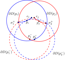
Figure 14: Illustration of the proof that $\gamma_{i}^{-}$ and $\gamma^{-}_{j}$ intersect exactly once (see Lemma 3.8).

Lemma 3.8.

Let $e_{i},e_{j}\in E_{t}$ be two distinct edges with $i<j$. Then the lower arcs $\gamma_{i}^{-}$ and $\gamma^{-}_{j}$ intersect in exactly one point and the two arcs cross at that point. Furthermore, $\gamma_{i}^{-}$ (resp. $\gamma_{j}^{-}$) appears on $\mathscr{L}(\{\gamma_{i}^{-},\gamma_{j}^{-}\})$ only before (resp. after) their intersection point.

Proof.

First, we observe that if $e_{i}$ and $e_{j}$ have a common endpoint $q$, then $q$ does not contribute to $\mathscr{L}(\{\gamma_{i}^{-},\gamma^{-}_{j}\})$, i.e., the unit disc $D(q)$ lies strictly above $\mathscr{L}(\{\gamma_{i}^{-},\gamma^{-}_{j}\})$. Indeed, assume for a contradiction that $\mathscr{L}(\{\gamma_{i}^{-},\gamma^{-}_{j}\})$ contains a point $r$ with distance $1$ from $q$. Then, the unit disc $D(r)$ is tangent to $e_{i}$ and $e_{j}$ at the point $q$. However, this is impossible, since $e_{i}$ and $e_{j}$ belong to the lower semi-circles of two distinct unit discs.

Next, notice that the arcs $\gamma_{i}^{-}$ and $\gamma^{-}_{j}$ intersect at least once since any two points in the grid cell $C$ have distance at most $1$. Suppose $p^{-}_{1}$ is a point on $\gamma_{j}^{-}$ and $p^{-}_{2}$ a point on $\gamma_{i}^{-}$, with $p^{-}_{1}<_{x}p^{-}_{2}$; refer to Figure 14. Assume for a contradiction that both $p^{-}_{1}$ and $p^{-}_{2}$ appear on $\mathscr{L}(\{\gamma_{i}^{-},\gamma^{-}_{j}\})$. Consider the upper semi-circle $\sigma_{1}^{+}$ of $D(p_{1}^{-})$ and the upper semi-circle $\sigma_{2}^{+}$ of $D(p_{2}^{-})$. The upper semi-circle $\sigma_{1}^{+}$ touches $e_{j}$ in a point $p_{j}$, and the upper semi-circle $\sigma_{2}^{+}$ touches $\partial D(p_{1}^{-})$ in a point $p_{i}$. Since $p_{1},p_{2}$ lie on the lower semicircles of $\partial D(p_{j}),\partial D(p_{i})$, respectively, and $\|p_{i}-p_{j}\|\leq 1$, the upper semi-circles $\sigma^{+}_{1}$ and $\sigma^{+}_{2}$ intersect exactly once, and since $p^{-}_{1}<_{x}p^{-}_{2}$, the semi-circle $\sigma^{+}_{1}$ appears to the left of $\sigma^{+}_{2}$ on the upper envelope $\mathscr{U}$ of $\sigma^{+}_{1}$ and $\sigma^{+}_{2}$. The point $p_{i}$ must be on $\mathscr{U}$, since otherwise $p^{-}_{1}$ would be inside $D(p_{i})$, which contradicts the fact that $p^{-}_{1}$ belongs to $\mathscr{L}(\{\gamma_{i}^{-},\gamma^{-}_{j}\})$; and similarly for $p_{j}$. This implies that $p_{i}\geq_{x}p_{j}$. Now, recall that the common endpoint of $e_{i}$ and $e_{j}$ (if it exists) does not contribute to $\mathscr{L}(\{\gamma_{i}^{-},\gamma^{-}_{j}\})$, so we actually have $p_{i}>_{x}p_{j}$, which contradicts the assumption $i<j$. Thus, it follows that $\gamma_{i}^{-}$ and $\gamma_{j}^{-}$ intersect exactly once and that $\gamma_{i}^{-}$ appears before $\gamma_{j}^{-}$ on $\mathscr{L}(\{\gamma_{i}^{-},\gamma^{-}_{j}\})$. Furthermore, this argument also implies that $\gamma_{i}^{-}$ lies above $\gamma_{j}^{-}$ after their intersection point and vice-versa. We can conclude that $\gamma_{i}^{-}$ (resp., $\gamma_{j}^{-}$) appears on $\mathscr{L}(\{\gamma_{i}^{-},\gamma^{-}_{j}\})$ only before (resp., after) their intersection point. ∎

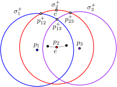
Figure 15: Illustration of the proof of Lemma 3.9.

Lemma 3.9.

Let $e_{i}$, $e_{j}$, and $e_{h}$, for $i<j<h$, be three edges in $E_{t}$, and let $q\in\mathbb{R}^{2}$ be a point. If $q$ is below $\gamma_{i}^{+}$ and $\gamma^{+}_{h}$ then $q$ is also below $\gamma^{+}_{j}$. Furthermore, for every endpoint $p$ of every edge of $E_{t}$, the upper semi-circle of $D(p)$ appears on $\mathscr{U}(\Gamma^{+})$. The $x$-order of the arcs on $\mathscr{U}(\Gamma^{+})$ corresponds to the $x$-order of the endpoints of the edges of $E_{t}$.

Proof.

Let $p_{1}$, $p_{2}$, and $p_{3}$ be points on three distinct edges of $E_{t}$, with $p_{1}<_{x}p_{2}<_{x}p_{3}$; see Figure 15. Let $\sigma^{+}_{1}$, $\sigma^{+}_{2}$, and $\sigma^{+}_{3}$ be the upper semi-circles of $D(p_{1})$, $D(p_{2})$, and $D(p_{3})$, respectively. Let $p^{+}_{12}$ and $p^{+}_{23}$ be the intersection points $\sigma^{+}_{1}\cap\sigma^{+}_{2}$ and $\sigma^{+}_{2}\cap\sigma^{+}_{3}$, respectively. Note that these intersection points exist, since the distance between any two points in the grid cell $C$ is at most 1. Since $p_{1}<_{x}p_{2}$, we have that $\sigma^{+}_{1}$ appears to the left of $\sigma^{+}_{2}$ on $\mathscr{U}(\{\sigma^{+}_{1},\sigma^{+}_{2}\})$. Let $c$ be the center of the circle containing the edge $e$ of $E_{t}$ that contains $p_{2}$. The point $c$ is on $\sigma^{+}_{2}$, since $p_{2}$ belongs to a lower semi-circle of radius 1. Moreover, $c$ is not below $\sigma^{+}_{1}$, since otherwise we would have that $p_{1}$ is in the interior of $D(c)$, contradicting the fact that $p_{1}$ lies on an edge of $E_{t}$. This means that $p^{+}_{12}\leq_{x}c$. The same argument implies that $p^{+}_{23}\geq_{x}c$ and therefore $p^{+}_{12}\leq_{x}p^{+}_{23}$. This in turn implies that the intersection point, $p^{+}_{13}$, between $\sigma^{+}_{1}$ and $\sigma^{+}_{3}$ is below or on $\sigma^{+}_{2}$ and therefore every point that lies below $\sigma^{+}_{1}$ and $\sigma^{+}_{3}$ also lies below $\sigma^{+}_{2}$.

The lemma readily follows from the above observations. ∎

Next, we show that for any two distinct edges $e_{i},e_{j}\in E_{t}$, the upper arc $\gamma_{i}^{+}$ and the lower arc $\gamma^{-}_{j}$ are disjoint. Furthermore, we show that $\gamma_{i}^{+}$ is above $\gamma^{-}_{j}$, hence proving Property (P3).

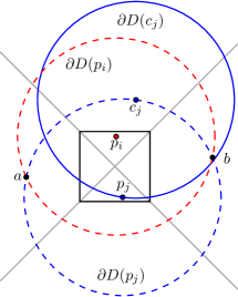
Figure 16: Illustration of the proof that $\gamma_{i}^{-}$ and $\gamma^{+}_{j}$ do not intersect (Lemma 3.10).

Lemma 3.10.

Let $e_{i}$ and $e_{j}$ be two distinct edges in $E_{t}$, and let $\ell$ be a vertical line. If $\ell$ intersects with $\gamma_{i}^{+}$ and $\gamma^{-}_{j}$ in the points $p$ and $q$, respectively, then, $p>_{y}q$.

Proof.

First, we show that $\gamma_{i}^{-}$ and $\gamma^{+}_{j}$ do not intersect. Suppose for a contradiction that $\gamma_{i}^{-}$ and $\gamma^{+}_{j}$ intersect at a point $a$. This means that $a$ is one of the intersection points of $\partial D(p_{i})$ and $\partial D(p_{j})$, where $p_{i}\in e_{i}$ and $p_{j}\in e_{j}$. Then $a\leq_{y}p_{i}$ and $a\geq_{y}p_{j}$, since $a$ lies on $\gamma_{i}^{-}$ and on $\gamma^{+}_{j}$. The same argument applies to the second intersection point, $b$, between $\partial D(p_{i})$ and $\partial D(p_{j})$. Assume that $a<_{x}b$, which implies that $a$ and $b$ belong to $Q_{l}$ and $Q_{r}$, respectively. Let $c_{j}$ be the center point of $e_{j}$. The point $c_{j}$ lies on the upper semi-circle of $D(p_{j})$, and it belongs to $Q_{t}$ which means that $c_{j}\in D(p_{i})$. This means that $p_{i}\in D(c_{j})$ which contradicts the fact that $e_{i}$ belongs to $E_{t}$; see Figure 16.

Since $\gamma_{i}^{+}$ and $\gamma^{-}_{j}$ do not intersect, it must be that that in the common $x$-interval of $\gamma_{i}^{+}$ and $\gamma^{-}_{j}$, the arc $\gamma_{i}^{+}$ is strictly above or below $\gamma^{-}_{j}$. The edge $e_{i}$ is above $\gamma^{-}_{j}$ and therefore $\gamma_{i}^{+}$ is above $\gamma^{-}_{j}$. ∎

4 Intersection Searching of Unit Arcs with a Unit Disc

In this section, we address the following intersection-searching problem: Preprocess a collection $\mathscr{C}$ of circular arcs of unit radius into a data structure so that for a query point $x\in\mathbb{R}^{2}$, the arcs in $\mathscr{C}$ intersecting the unit disc $D(x)$ can be reported efficiently. By splitting each arc of $\mathscr{C}$ into at most three arcs, we can ensure that each arc of $\mathscr{C}$ lies in the lower or upper semi-circle of its supporting disc. We assume for simplicity that every arc in $\mathscr{C}$ belongs to the lower semi-circle of its supporting disc. A similar data structure can be constructed for arcs lying in upper semi-circles.

Let $e\in\mathscr{C}$ be a unit-radius circular arc whose center is at $c$, and let $p_{1}$ and $p_{2}$ be its endpoints. A unit disc $D(x)$ intersects $e$ if and only if $e\oplus D(0)$, the Minkowski sum of $e$ with a unit disc at the origin, contains the center $x$. Let $z=D(p_{1})\cup D(p_{2})$, and let $D^{+}(c)$ be the disc of radius $2$ centered at $c$; $z$ divides $D^{+}(c)$ into three regions (see Figure 17): (i) $z^{+}$, the portion of $D^{+}(c)\setminus z$ above $z$, (ii) $z$ itself, and (iii) $z^{-}$, the portion of $D^{+}(c)\setminus z$ below $z$. It can be verified that $e\oplus D(0)=z\cup z^{-}$. We give an alternate characterization of $z\cup z^{-}$, which will help in developing the data structure.

Let $\ell$ be a line that passes through the tangent points, $p^{\prime}_{1}$ and $p^{\prime}_{2}$, of $D(p_{1})$ and $D(p_{2})$ with $D^{+}(c)$, respectively, and let $\ell^{-}$ be the halfplane below $\ell$. Set $L(e)=D^{+}(c)\cap\ell^{-}$.

Lemma 4.1.

If $\partial D(p_{1})$ and $\partial D(p_{2})$ intersect at two points (one of which is always $c$), then $\ell$ passes through $q=(\partial D(p_{1})\cap\partial D(p_{2}))\setminus\{c\}$. Otherwise, $c\in\ell$.

Proof.

Assume that $q$ exists. The quadrilateral $(c,p_{1},q,p_{2})$ is a rhombus, since all its edges have length $1$. Let $\alpha$ be the angle $\angle p_{1}qp_{2}$ and $\beta$ be the angle $\angle cp_{1}q$. The angle $\angle qp_{1}p^{\prime}_{1}$ is equal to $\alpha$, since the segment $(c,p^{\prime}_{1})$ is a diameter of $D(p_{1})$. The angle $\angle p_{1}qp^{\prime}_{1}$ is equal to $\frac{\beta}{2}$, since $\triangle p_{1}qp^{\prime}_{1}$ is an isosceles triangle. The same arguments apply to the angle $\angle p_{2}qp^{\prime}_{2}$, implying that the angle $\angle p^{\prime}_{1}qp^{\prime}_{2}$ is equal to $\pi$.

Assume now that $q$ does not exist. Then the segment $(p_{1},p_{2})$ is a diameter of $D(c)$. The segment $(c,p^{\prime}_{1})$ is a diameter of $D(p_{1})$. The segment $(p_{1},p_{2})$ coincides with $(c,p^{\prime}_{1})$ at the segment $(c,p_{1})$. The same argument applies to the segment $(c,p^{\prime}_{2})$, implying that the angle $\angle p^{\prime}_{1}qp^{\prime}_{2}$ is equal to $\pi$. ∎

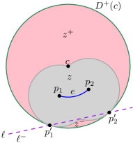
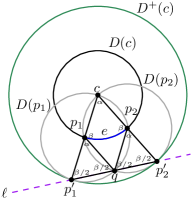
Figure 17: (On the left) Partition of $D^{+}(c)$ into three regions: $z^{+}$, $z$ and $z^{-}$. (On the right) Illustration of Lemma 4.1.

The following corollary summarizes the criteria for the intersection of a unit circular arc with a unit disc.

Corollary 4.2.

Let $e$ be a circular arc in $\mathscr{C}$ with endpoints $p_{1}$ and $p_{2}$ and center $c$. Then $z\cup z^{-}=z\cup L(e)$. Furthermore, $e$ intersects a unit disc $D(x)$ if and only if at least one of the following conditions is satisfied: (i) $x\in D(p_{1})$ (or $p_{1}\in D(x)$), (ii) $x\in D(p_{2})$ (or $p_{2}\in D(x)$), and (iii) $x\in L(e)$.

We thus construct three separate data structures. The first data structure preprocesses the left endpoints of the arcs in $\mathscr{C}$ for unit-disc range searching, the second data structure preprocesses the right endpoints of arcs in $\mathscr{C}$ for unit-disc range searching, and the third data structure preprocesses $\mathscr{L}=\{L(e)\mid e\in\mathscr{C}\}$ for inverse range searching, i.e., reporting all regions in $\mathscr{L}$ that contain a query point. Using standard disk range-searching data structures (see e.g. [3, 2]), we can build these three data structures so that each of them takes $O(n)$ space and answers a query in $O(n^{1/2+\varepsilon}+k)$ time, where $k$ is the output size. Furthermore, these data structures can handle insertions/deletions in $O(\log^{2}n)$ time using the lazy-partial-rebuilding technique [26]. We conclude the following:

Theorem 4.3.

Let $\mathscr{C}$ be a set of $n$ unit-circle arcs in $\mathbb{R}^{2}$. Then, $\mathscr{C}$ can be preprocessed into a data structure of linear size so that for a query unit disc $D$, all arcs of $\mathscr{C}$ intersecting $D$ can be reported in $O(n^{1/2+\varepsilon}+k)$ time, where $\varepsilon$ is an arbitrarily small constant and $k$ is the output size. Furthermore the data structure can be updated under insertion/deletion of a unit-circle arc in $O(\log^{2}n)$ amortized time.

5 Conclusion

In this paper, we presented linear-size dynamic data structures for maintaining the union of unit discs under insertions and for maintaining the lower envelope of pseudo-lines in the plane under both insertions and deletions. We also presented a linear-size structure for storing a set of circular arcs of unit radius (not necessarily on the boundary of the union of the corresponding discs), so that all input arcs intersecting a query unit disc can be reported quickly. We conclude by mentioning a few open problems:

• Can the boundary of the union of unit discs be maintained in an output-sensitive manner when we allow both insertions and deletions of discs? The challenge in extending our data structure to handle the deletion of a unit disc $D$ is to quickly report the new edges of $\mathscr{U}$ that lie in the interior of $D$.

• Can our data structure be extended to maintain the boundary of the union of discs of arbitrary radii? Although the union boundary still has linear size, many of the structure properties of the union used by our data structure no longer hold, e.g., two upper (or lower) arcs may intersect at two points and they cannot be treated as pseudo-lines.

• Can the area of the union of unit discs be maintained under insertions and deletions in sublinear time per update? As mentioned in the introduction, it is not clear how to extend Chan’s data structure [15] for maintaining the volume of the convex hull of a set of points in $\mathbb{R}^{3}$ to our setting.

Acknowledgments.

We thank Haim Kaplan and Micha Sharir for helpful discussions, and reviewers for their useful comments.

Appendix: An example run of the algorithm in Section 2.3

In this appendix we illustrate the algorithm, described in Section 2.3, for computing the intersection point of the lower envelopes of two sets of pseudo-lines such that all lines in one set are smaller than all in the other set.

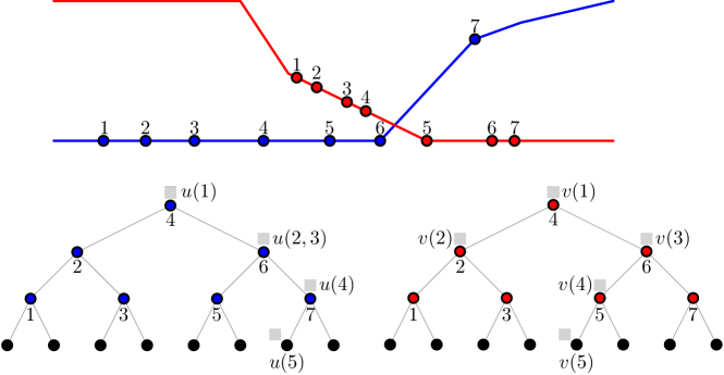
Figure 19: Top: the two lower envelopes $\mathscr{L}_{l}$ and $\mathscr{L}_{r}$ for the pseudo-lines in Figure 18. Bottom: the corresponding trees $\Lambda_{l}$ and $\Lambda_{r}$. The labels $u(i)$ and $v(i)$ indicate the position of the pointers $u$ and $v$ at step $i$, during the search.

Step	$u$	$v$	uStack	vStack	Procedure case
1	4	4	$\emptyset$	$\emptyset$	Case 3
2	6	2	4	4	Case 2 $\rightarrow$ Case 2
3	6	6	4	$\emptyset$	Case 3
4	7	5	4, 6	6	Case 1 $\rightarrow$ Case 3
5	7*	5*	4, 6	6, 5	Case 3 $\rightarrow$ End

Table 1: The progress of the search for the example in Figure 19.

References

- [1] P. K. Agarwal. Range searching. In J. E. Goodman, J. O’Rourke, and C. Tóth, editors, Handbook of Discrete and Computational Geometry, chapter 40, pages 1057–1092. CRC Press, 3rd edition, 2017.
- [2] P. K. Agarwal. Simplex range searching and its variants: A review. In M. Loebl, J. Nešetřil, and R. Thomas, editors, A Journey Through Discrete Mathematics: A Tribute to Jiří Matoušek, pages 1–30. Springer-Verlag, 2017.
- [3] P. K. Agarwal and J. Matoušek. On range searching with semialgebraic sets. Discrete Comput. Geom., 11(4):393–418, 1994.
- [4] P. K. Agarwal and J. Matoušek. Dynamic half-space range reporting and its applications. Algorithmica, 13(4):325–345, 1995.
- [5] P. K. Agarwal, M. Pellegrini, and M. Sharir. Counting circular arc intersections. SIAM J. Comput., 22(4):778–793, 1993.
- [6] P. K. Agarwal, M. J. van Kreveld, and M. H. Overmars. Intersection queries in curved objects. J. Algorithms, 15(2):229–266, 1993.
- [7] F. Aurenhammer. Improved algorithms for discs and balls using power diagrams. J. Algorithms, 9(2):151–161, 1988.
- [8] J. L. Bentley and J. B. Saxe. Decomposable searching problems I: Static-to-dynamic transformation. J. Algorithms, 1(4):301–358, 1980.
- [9] M. de Berg, K. Buchin, B. M. P. Jansen, and G. J. Woeginger. Fine-grained complexity analysis of two classic TSP variants. ACM Transactions on Algorithms, 17(1):5:1–5:29, 2021.
- [10] M. de Berg, O. Cheong, M. J. van Kreveld, and M. H. Overmars. Computational Geometry: Algorithms and Applications, 3rd edition. Springer, 2008.
- [11] G. S. Brodal and R. Jacob. Dynamic planar convex hull with optimal query time. In Proc. 7th Scandinavian Workshop on Algorithm Theory (SWAT), pages 57–70, 2000.
- [12] G. S. Brodal and R. Jacob. Dynamic planar convex hull. In Proc. 43rd Annu. IEEE Sympos. Found. Comput. Sci. (FOCS), pages 617–626, 2002.
- [13] T. M. Chan. Dynamic planar convex hull operations in near-logarithmaic amortized time. J. ACM, 48(1):1–12, 2001.
- [14] T. M. Chan. A dynamic data structure for 3-d convex hulls and 2-d nearest neighbor queries. J. ACM, 57(3):16:1–16:15, 2010.
- [15] T. M. Chan. Dynamic geometric data structures via shallow cuttings. Discrete Comput. Geom., 64(4):1235–1252, 2020.
- [16] R. Cohen, Y. Yovel, and D. Halperin. Sensory regimes of effective distributed searching without leaders. arXiv:1904.02895, 2019.
- [17] S. Felsner and J. E. Goodman. Pseudoline arrangements. In J. E. Goodman, J. O’Rourke, and C. D. Tóth, editors, Handbook of Discrete and Computational Geometry, chapter 5, pages 83–109. CRC Press, 3rd edition, 2017.
- [18] B. Grünbaum. Arrangements and Spreads. Conference Board of the Mathematical Sciences, 1972.
- [19] P. Gupta, R. Janardan, and M. H. M. Smid. On intersection searching problems involving curved objects. In Proc. 4th Scandinavian Workshop on Algorithm Theory (SWAT), pages 183–194, 1994.
- [20] D. Halperin and M. Sharir. Arrangements. In J. E. Goodman, J. O’Rourke, and C. D. Tóth, editors, Handbook of Discrete and Computational Geometry, chapter 28, pages 1343–1376. CRC Press, 3rd edition, 2017.
- [21] J. Hershberger and S. Suri. Finding tailored partitions. J. Algorithms, 12(3):431–463, 1991.
- [22] H. Kaplan, W. Mulzer, L. Roditty, P. Seiferth, and M. Sharir. Dynamic planar Voronoi diagrams for general distance functions and their algorithmic applications. Discrete Comput. Geom., 64(3):838–904, 2020.
- [23] H. Kaplan, R. E. Tarjan, and K. Tsioutsiouliklis. Faster kinetic heaps and their use in broadcast scheduling. In Proc. 12th Annu. ACM-SIAM Sympos. Discrete Algorithms (SODA), pages 836–844, 2001.
- [24] K. Kedem, R. Livne, J. Pach, and M. Sharir. On the union of Jordan regions and collision-free translational motion amidst polygonal obstacles. Discrete Comput. Geom., 1:59–70, 1986.
- [25] C.-H. Liu. Nearly optimal planar nearest neighbors queries under general distance functions. In Proc. 31st Annu. ACM-SIAM Sympos. Discrete Algorithms (SODA), pages 2842–2859, 2020.
- [26] M. H. Overmars. The Design of Dynamic Data Structures, volume 156 of Lecture Notes in Computer Science. Springer-Verlag, 1983.
- [27] M. H. Overmars and J. van Leeuwen. Maintenance of configurations in the plane. J. Comput. System Sci., 23(2):166–204, 1981.
- [28] F. P. Preparata. An optimal real-time algorithm for planar convex hulls. Commun. ACM, 22(7):402–405, 1979.
- [29] F. P. Preparata and M. I. Shamos. Computational Geometry. An Introduction. Springer-Verlag, 1985.
- [30] P. G. Spirakis. Very fast algorithms for the area of the union of many circles. Technical Report 98, Courant Institute, New York University, 1983.
- [31] R. E. Tarjan. Data structures and network algorithms. SIAM, 1983.