Hybrid classical-quantum linear solver using Noisy Intermediate-Scale Quantum machines

Abstract

We propose a realistic hybrid classical-quantum linear solver to solve systems of linear equations of a specific type, and demonstrate its feasibility with Qiskit on IBM Q systems. This algorithm makes use of quantum random walk that runs in $\mathcal{O}(N\log(N))$ time on a quantum circuit made of $\mathcal{O}(\log(N))$ qubits. The input and output are classical data, and so can be easily accessed. It is robust against noise, and ready for implementation in applications such as machine learning.

I Introduction

Algorithms that run on quantum computers hold promise to perform important computational tasks more efficiently than what can ever be achieved on classical computers, most notably Grover’s search algorithm and Shor’s integer factorization Nielsen and Chuang (2011). One computational task indispensable for many problems in science, engineering, mathematics, finance, and machine learning, is solving systems of linear equations $\textbf{A}\vec{x}=\vec{b}$. Classical direct and iterative algorithms take $\mathcal{O}(N^{3})$ and $\mathcal{O}(N^{2})$ time Golub and Van Loan (1996); Saad (2003). Interestingly, the Harrow-Hassidim-Lloyd (HHL) quantum algorithm Harrow et al. (2009); Clader et al. (2013); Montanaro and Pallister (2016); Childs et al. (2017); Costa et al. (2019); Berry et al. (2017); Dervovic et al. (2018); Wossnig et al. (2018); Biamonte et al. (2017); Ciliberto et al. (2018), which is based on the quantum circuit model Deutsch (1985), takes only $\mathcal{O}(\log(N))$ to solve a sparse $N\times N$ system of linear equations, while for dense systems it requires $\mathcal{O}(\sqrt{N}\log(N))$ Wossnig et al. (2018). Linear solvers and experimental realizations that use quantum annealing and adiabatic quantum computing machines Kadowaki and Nishimori (1998); Farhi et al. (2000); Aharonov et al. (2008) are also reported O’Malley and Vesselinov (2016); Borle and Lomonaco (2018); Chang et al. (2018). Most recently, methods Wen et al. (2019); Subaş ı et al. (2019) inspired by adiabatic quantum computing are proposed to be implemented on circuit-based quantum computers. Whether substantial quantum speedup exists in these algorithms remains unknown.

In practice, the applicability of quantum algorithms to classical systems are limited by the short coherence time of noisy quantum hardware in the so-called Noisy Intermediate-Scale Quantum (NISQ) era Preskill (2018) and the difficulty in executing the input and output of classical data. Other roadblocks toward practical implementation include limited number of qubits, limited connectivity between qubits, and large error correction overhead. At present, experiments demonstrating the HHL linear solver on circuit quantum computers are limited to $2\times 2$ matrices Cao et al. (2012); Cai et al. (2013); Barz et al. (2014); Pan et al. (2014); Zheng et al. (2017); Lee et al. (2019), while linear solvers inspired by adiabatic quantum computing are limited to $8\times 8$ matrices Wen et al. (2019); Subaş ı et al. (2019). For quantum annealers, the state-of-the-art linear solvers can solve up to $12\times 12$ matrices Chang et al. (2018).

In addition to the problems of limited available entangled qubits and short coherence time, the HHL-type algorithms are designed to work only when input and output are quantum states Aaronson (2015). This condition imposes severe restriction to practical applications in the NISQ era Childs (2009); Aaronson (2015); Preskill (2018). It has been shown that the HHL algorithm can not extract information about the norm of the solution vector $\vec{x}$ Harrow et al. (2009). A state preparation algorithm for inputting a classical vector $\vec{b}$ would take $\mathcal{O}(N)$ time Möttönen et al. (2004); Plesch and Brukner (2011); Aaronson (2015); Coles et al. (2018), with large overhead for current hardware. In addition, quantum state tomography is required to read out the classical solution vector $\vec{x}$, which is a demanding task James et al. (2001); Suess et al. (2017), except for special cases like one-dimensional entangled qubits Cramer et al. (2010). Inputting the matrix A is also a challenge that may kill the quantum speedup Nielsen and Chuang (2011); Cao et al. (2012); Cai et al. (2013); Barz et al. (2014); Pan et al. (2014); Zheng et al. (2017); Lee et al. (2019).

In this work, we propose a hybrid classical-quantum linear solver that uses circuit-based quantum computer to perform quantum random walks. In contrast to the HHL-type linear solvers, the solution vector $\vec{x}$ and the constant vector $\vec{b}$ in this hybrid algorithm stay as classical data in the classical registers. Only the matrix A is encoded in quantum registers. The idea is similar to that of variational quantum eigensolvers Peruzzo et al. (2014); Wecker et al. (2015); McClean et al. (2016); Kandala et al. (2017), where quantum speedup is exploited only for sampling exponentially large state Hilbert spaces, while the rest of computational task is done by classical computer. This makes it easy to perform data input and output: the $\vec{b}$ vector can be arbitrary, and the components and the norm of the $\vec{x}$ vector can be easily accessed.

We consider matrices that are useful for Markov decision problems such as in reinforcement learning Sutton and Barto (1998). We show that these matrices can be efficiently encoded by introducing the Hamming cube structure: a square matrix of size $N$ requires $\mathcal{O}(\log(N))$ quantum bits only. The quantum random walk algorithm we here propose takes $\mathcal{O}(\log(N))$ time to obtain one component of the $\vec{x}$ vector. We also show that in the quantum random walk algorithm the matrices produced as a result of qubit-qubit correlation are inherently complex, which can be an advantage for performing difficult tasks. For the same amount of time, the matrices the classical random walk algorithm can solve are limited to factorisable ones only.

We have tested the quantum random walk algorithm using software development kit Qiskit on IBM Q systems Aleksandrowicz et al. (2019); IBM (2016). Numerical results show that this linear solver works on ideal quantum computer, and most importantly, also on noisy quantum computer having a short coherence time, provided the quantum circuit that encodes the A matrix is not too long. The limitation due to machine errors is discussed.

II Methods

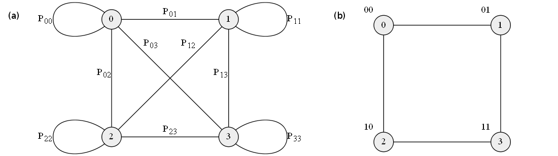
Figure 1: (a) Quantum (or classical) random walk on an undirected $N=4$ graph. The transition probability of going from node $I$ to node $J$ or vice versa is equal to $P_{I,J}$, these elements forming a $4\times 4$ matrix. (b) The four nodes on this Hamming cube are labeled by integers $(0,1,2,3)$; they are encoded as four different states $|00\rangle$, $|01\rangle$, $|10\rangle$, $|11\rangle$, respectively.

We consider a system of linear equations of real numbers $\textbf{A}\vec{x}=\vec{b}$, where A is a $N\times N$ matrix to be solved, $N\times 1$ vectors $\vec{x}$ and $\vec{b}$ are, respectively, the solution vector and a vector of constants. Without loss of generality, we rewrite A as

$$\textbf{A}=\mathbf{1}-\gamma\textbf{P}\,,$$ (1)

where $\mathbf{1}$ is the identity matrix, and $0<\gamma<1$ is a real number. We take P as a (stochastic) Markov-chain transition matrix, such that $P_{I,J}\geq 0$ and $\sum_{J}P_{I,J}=1$, where $P_{I,J}$ refers to the P matrix element in the $J$-th column of the $I$-th row. This type of linear systems appears in value estimation for reinforcement learning Barto and Duff (1993); Sutton and Barto (1998); Paparo et al. (2014), and radiosity equation in computer graphics Goral et al. (1984). In reinforcement learning algorithms, given a fixed policy of the learning agency, the vector $\vec{x}$ is the value function that determines the long-term cumulative reward, and efficient estimation of this function is key to successful learning Sutton and Barto (1998). Note that the matrix A given in Eq. (1) used as model Hamiltonian matrix belongs to the so-called stoquastic Hamiltonians Bravyi et al. (2008); Bravyi (2015).

To solve $\textbf{A}\vec{x}=\vec{b}$, we expand the solution vector as Neumann series, that is, $\vec{x}=\textbf{A}^{-1}\vec{b}=(\mathbf{1}-\gamma\textbf{P})^{-1}\vec{b}=\sum_{s=0}^{\infty}\gamma^{s}\textbf{P}^{s}\vec{b}$. Let us define the $I_{0}$ component of $\vec{x}$ truncated up to $\gamma^{c}$ terms as

$$x^{(c)}_{I_{0}}=\sum_{s=0}^{c}\gamma^{s}\sum_{I_{1},...,I_{s}=1}^{N}P_{I_{0},I_{1}}...P_{I_{s-1},I_{s}}b_{I_{s}}\,.$$ (2)

This expression for $x^{(c)}_{I_{0}}$ can be evaluated by random walks on a graph of $N$ nodes, with the probability of going from node $I$ and node $J$ of the graph given by the matrix element $P_{I,J}$, which we set as symmetric (undirected), namely $P_{I,J}=P_{J,I}$. An example of a four-node graph is shown in Fig. 1(a). By performing a series of random walks starting from node $I_{0}$, walking $c$ steps according to the transition probability matrix P, and ending at some node $I_{c}$, Eq. (2) can be readily calculated to get the $x^{(c)}_{I_{0}}$ value, which is close to the solution $x_{I_{0}}$ for some large $c$ steps. Truncating the series introduces an error $\epsilon\sim\mathcal{O}(\gamma^{c})$. So, for a given $\gamma$, the number of steps necessary to meet a given tolerance $\epsilon$ is equal to $c\sim\log(1/\epsilon)/\log(1/\gamma)$.

The above expansion procedure can be extended to more general matrices A by setting $\textbf{A}=\mathbf{1}-\textbf{B}$ where $B_{I,J}=P_{I,J}v_{I,J}$ for real matrix elements $v_{I,J}$ provided that the eigenvalues of B are bounded by $-1<\mbox{eig}(\textbf{B})_{I}<1$.

For classical Monte Carlo methods to compute Eq. (2), it takes $\mathcal{O}(N)$ time to calculate the cumulative distribution function that is used to determine the next walking step. So, these linear systems can be solved by classical Monte Carlo methods within $\mathcal{O}(N^{2})$ time Metropolis and Ulam (1949); Forsythe and Leibler (1950); Wasow (1952); Lu and Schuurmans (2003); Branford et al. (2008). Similar Monte Carlo methods have been extended to more general matrices for applications in Green’s function Monte Carlo method for many-body physics Ceperley and Alder (1980); Negele and Orland (1988); Landau and Binder (2005).

II.1 Encoding state spaces on Hamming cubes

As for material resources, in general it takes at least $\mathcal{O}(N)$ classical bits to store a row of a stochastic transition matrix P (or A). However, for the classical and quantum random walks we here consider, it is possible to reduce significantly the number of classical or quantum bits necessary to encode the corresponding transition probability matrix P to $\mathcal{O}(\log(N))$ by introducing the Hamming cube (HC) structure Hamming (1950). To do it, we first associate each graph node with a bit string. As shown in Fig. 1(b), the four nodes of the $N=4$ graph are fully represented by two bits. Node states $|0\rangle$, $|1\rangle$, $|2\rangle$, and $|3\rangle$ represent binary string states $|00\rangle$, $|01\rangle$, $|10\rangle$, and $|11\rangle$, respectively. For a $N$-node graph, only $\log_{2}(N)=n$ (to base 2) bits are needed to encode the integers $J\in\{0,1,...,N{-}1\}$, each representing the $n$-bit binary string state, namely $|J\rangle=|j_{n-1},...j_{1},j_{0}\rangle$, where $j_{\ell}$ is 0 or 1.

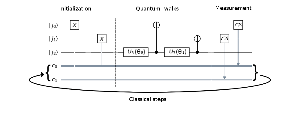
Figure 2: Discrete-time coined quantum walk circuit for the $4\times 4$ transition matrix given in Eq. (10). Qubits $j_{0}$ and $j_{1}$ are state register qubits to represent the four-node graph in Fig. 1, first set as $0$ before initialization, while the qubit $j_{2}$ is the coin register qubit. The measured registers $c_{0}$ and $c_{1}$ are fed back to initialize the next iteration. The classical-step is repeated $c$ times to obtain the Neumann expansion up to order $c$.

II.2 Classical random walk

Before we introduce our quantum random walk algorithm, let us first consider classical random walks.

To perform random walks on a $N$-node graph, we use a simple coin-flipping process with $\mathcal{O}(\log(N))$ time steps. The $\ell$-th bit flips with probability $\sin^{2}(\theta_{\ell}/2)$ or does not flip with probability $\cos^{2}(\theta_{\ell}/2)$, the total probability being equal to 1. The transition probability matrix elements are given by

$$P^{classical}_{J^{\prime},J}=\prod_{\ell=0}^{n-1}\Big{|}\cos^{2}(\frac{\theta_{\ell}}{2})\Big{|}^{1-i_{\ell}}\Big{|}\sin^{2}(\frac{\theta_{\ell}}{2})\Big{|}^{i_{\ell}},$$ (3)

where the $n$-bit binary string state $|I\rangle_{c}=|i_{n-1},...,i_{1},i_{0}\rangle_{c}$ is determined by $|J^{\prime}\rangle_{c}=|I\rangle_{c}\oplus|J\rangle_{c}$, where $\oplus$ denotes the bitwise exclusive or (XOR) operation, and the subscript $c$ denotes classical states. The total number of $|\sin^{2}(\theta_{\ell}/2)|$, given by $d^{classical}=\sum_{\ell=0}^{n-1}i_{\ell}$, is the Hamming weight of $|I\rangle_{c}$, and so corresponds to the Hamming distance between $|J^{\prime}\rangle_{c}$ and $|J\rangle_{c}$ states. This metric measures the number of steps that a walker needs to go from $|J\rangle_{c}$ to $|J^{\prime}\rangle_{c}$ on the Hamming cube.

For the four-node graph shown in Fig. 1, the transition probability matrix P for classical random walks reads

$$\textbf{P}^{classical} = \begin{bmatrix}\cos^{2}(\frac{\theta_{0}}{2})\cos^{2}(\frac{\theta_{1}}{2})&\sin^{2}(\frac{\theta_{0}}{2})\cos^{2}(\frac{\theta_{1}}{2})&\cos^{2}(\frac{\theta_{0}}{2})\sin^{2}(\frac{\theta_{1}}{2})&\sin^{2}(\frac{\theta_{0}}{2})\sin^{2}(\frac{\theta_{1}}{2})\\ &\cos^{2}(\frac{\theta_{0}}{2})\cos^{2}(\frac{\theta_{1}}{2})&\sin^{2}(\frac{\theta_{0}}{2})\sin^{2}(\frac{\theta_{1}}{2})&\cos^{2}(\frac{\theta_{0}}{2})\sin^{2}(\frac{\theta_{1}}{2})\\ &&\cos^{2}(\frac{\theta_{0}}{2})\cos^{2}(\frac{\theta_{1}}{2})&\sin^{2}(\frac{\theta_{0}}{2})\cos^{2}(\frac{\theta_{1}}{2})\\ &&&\cos^{2}(\frac{\theta_{0}}{2})\cos^{2}(\frac{\theta_{1}}{2})\\ \end{bmatrix}$$ (4)

$$= \begin{bmatrix}\cos^{2}(\frac{\theta_{1}}{2})&\sin^{2}(\frac{\theta_{1}}{2})\\ \sin^{2}(\frac{\theta_{1}}{2})&\cos^{2}(\frac{\theta_{1}}{2})\end{bmatrix}\otimes\begin{bmatrix}\cos^{2}(\frac{\theta_{0}}{2})&\sin^{2}(\frac{\theta_{0}}{2})\\ \sin^{2}(\frac{\theta_{0}}{2})&\cos^{2}(\frac{\theta_{0}}{2})\end{bmatrix},$$

where $\otimes$ denotes the Kronecker product. The lower triangular part of the matrix is omitted due to symmetry. This simple case demonstrates a general feature for classical transition probability matrix $\textbf{P}^{classical}$: the probability of flipping both bits is simply a product of the probabilities of flipping the $0$-th bit and the $1$-th bit in arbitrary order. For instance, $P^{classical}_{0,3}=P^{classical}_{|00\rangle,|11\rangle}=\sin^{2}(\theta_{0}/2)\sin^{2}(\theta_{1}/2)=P^{classical}_{|00\rangle,|01\rangle}P^{classical}_{|00\rangle,|10\rangle}$; similarly for the other $P^{classical}_{I,J}$’s. The fact that $\textbf{P}^{classical}$ can be factorized into a Kronecker product of the matrices of each individual bit indicates that each bit flips independently, as for a Markovian process.

II.3 Quantum random walk

We can simulate quantum walks Aharonov et al. (1993); Childs et al. (2001); Aharonov et al. (2001); Moore and Russell (2002); Szegedy (2004); Kendon (2006); Childs (2017) on a $N$-node graph to obtain the solution vector $\vec{x}$ from Eq. (2). To do it, we use discrete-time coined quantum walk circuit Košík and Bužek (2005); Shikano and Katsura (2010). The circuit for the four-node graph in Fig. 1 is shown in Fig. 2. The first two qubits $j_{0}$ and $j_{1}$ are state registers that will be initialized to encode the four-node graph, while the third qubit $j_{2}$ is the coin register.

To derive the quantum transition probability matrix on a graph of $N$ nodes, we consider the state space of the $(n+1)$-qubit circuit as spanned by $\{|i_{n}\rangle_{\diamond}\otimes|i_{n-1},...,i_{1},i_{0}\rangle_{q}\}$ with $n=\log_{2}(N)$: the $(n+1)$-th qubit registers the coin state $|i_{n}\rangle_{\diamond}$, and the other $n$ qubits encode the $N$-node graph. We take the convention that the rightmost bit is $i_{0}$. Given a $n$-bit string $(j_{n-1},...,j_{1},j_{0})$, the initialized quantum state reads

$$|\psi_{0,J}\rangle = |0\rangle_{\diamond}\otimes|j_{n-1},j_{n-2},...,j_{2},j_{1},j_{0}\rangle_{q}$$

$$= |0\rangle_{\diamond}\otimes|J\rangle_{q}\,.$$

Next we let the $|\psi_{0,J}\rangle$ state evolve in random walk: in each walking step, we toss the coin by rotating the coin qubit, and then flip a graph qubit by applying the CNOT gate. This process is repeated on all the $n$ qubits in the $|j_{n-1},j_{n-2},...,j_{2},j_{1},j_{0}\rangle_{q}$ state, starting with the 0-th qubit. The corresponding evolution operator reads

$$\mathcal{U}{=}\prod_{k=0}^{n-1}\ {}^{\prime}\Big{(}|0\rangle_{\diamond}\langle 0|_{\diamond}\otimes 1_{q}+|1\rangle_{\diamond}\langle 1|_{\diamond}\otimes X_{k}\Big{)}\cdot\Big{(}U_{3}({\bf u}_{k})\otimes 1_{q}\Big{)},$$ (6)

where the prime (^′) on the $\prod$ denotes that the $k=0$ operator applies first to the right, followed by the $k=1$ operator, and so on; the $1_{q}$ operator is an identity map on the $n$-qubit state $|J\rangle_{q}$, $X_{k}$ is a Pauli $X$ gate (the Pauli matrix $\sigma_{x}$) that acts on the $k$-th qubit, and $U_{3}({\bf u})$ is a single-qubit rotation operator

$$U_{3}({\bf u})=U_{3}(\theta,\phi,\lambda)=\begin{bmatrix}\cos(\frac{\theta}{2})&-e^{i\lambda}\sin(\frac{\theta}{2})\\ e^{i\phi}\sin(\frac{\theta}{2})&e^{i(\lambda+\phi)}\cos(\frac{\theta}{2})\\ \end{bmatrix}$$ (7)

that acts on the coin qubit state. Note that the first parentheses in Eq. (6) represents a CNOT gate. It is important to note that here we use one quantum coin only to decide on the Pauli $X$ gate operation over all the $n$ qubits, so the order of qubit operations plays a role in the determination of the transition probability matrix P.

The first step is to project $\mathcal{U}$ on $|\psi_{0,J}\rangle$, which leads to

$$\mathcal{U}|\psi_{0,J}\rangle=\sum^{1}_{i_{n{-}1},...,i_{0}=0}\prod_{\ell=0}^{n-1}U_{3}({\bf u}_{\ell})_{i_{\ell},i_{\ell-1}}$$

$$\times |i_{n-1}\rangle_{\diamond}\otimes|i_{n-1}\oplus j_{n-1},...,i_{1}\oplus j_{1},i_{0}\oplus j_{0}\rangle_{q}\,,$$

with $i_{-1}=0$. By tracing out the coin degree of freedom, we obtain the reduced density matrix for the graph and hence the probability matrix $P_{J^{\prime},J}=\langle J^{\prime}|\mbox{Tr}_{\diamond}[\mathcal{U}|\psi_{0J}\rangle\langle\psi_{0J}|\mathcal{U}^{\dagger}]|J^{\prime}\rangle$. The resulting quantum transition probability matrix elements then read

$$P^{quantum}_{J^{\prime},J} = \prod_{\ell=0}^{n-1}\Big{|}U_{3}({\bf u}_{\ell})_{i_{\ell},i_{\ell-1}}\Big{|}^{2}$$

$$= \prod_{\ell=0}^{n-1}\Big{|}\cos^{2}(\frac{\theta_{\ell}}{2})\Big{|}^{1-(i_{\ell}\oplus i_{\ell-1})}\Big{|}\sin^{2}(\frac{\theta_{\ell}}{2})\Big{|}^{i_{\ell}\oplus i_{\ell-1}},$$

where $|I\rangle_{q}=|i_{n-1},...,i_{1},i_{0}\rangle_{q}$ is determined by $|J^{\prime}\rangle_{q}=|I\rangle_{q}\oplus|J\rangle_{q}$. For one $\mathcal{U}$ quantum evolution, the complex phase factors $e^{i\phi_{\ell}}$ and $e^{i\lambda_{\ell}}$ play no role. We will see later that these phases come into play in the case of multiple evolutions $\mathcal{U}^{q}$.

To understand the transition probability matrix produced by the quantum walk circuit (Fig. 2), let us again consider the four-node graph in Fig. 1, where

$$\textbf{P}^{quantum}=\begin{bmatrix}\cos^{2}(\frac{\theta_{0}}{2})\cos^{2}(\frac{\theta_{1}}{2})&\sin^{2}(\frac{\theta_{0}}{2})\sin^{2}(\frac{\theta_{1}}{2})&\cos^{2}(\frac{\theta_{0}}{2})\sin^{2}(\frac{\theta_{1}}{2})&\sin^{2}(\frac{\theta_{0}}{2})\cos^{2}(\frac{\theta_{1}}{2})\\ &\cos^{2}(\frac{\theta_{0}}{2})\cos^{2}(\frac{\theta_{1}}{2})&\sin^{2}(\frac{\theta_{0}}{2})\cos^{2}(\frac{\theta_{1}}{2})&\cos^{2}(\frac{\theta_{0}}{2})\sin^{2}(\frac{\theta_{1}}{2})\\ &&\cos^{2}(\frac{\theta_{0}}{2})\cos^{2}(\frac{\theta_{1}}{2})&\sin^{2}(\frac{\theta_{0}}{2})\sin^{2}(\frac{\theta_{1}}{2})\\ &&&\cos^{2}(\frac{\theta_{0}}{2})\cos^{2}(\frac{\theta_{1}}{2})\\ \end{bmatrix}.$$ (10)

Unlike the above classical random walk, this matrix cannot be factorized into a Kronecker product of the matrices of each individual qubit. The probability of one qubit flipping depends on the other, indicating that the two qubits are correlated, or in quantum information theory entangled.

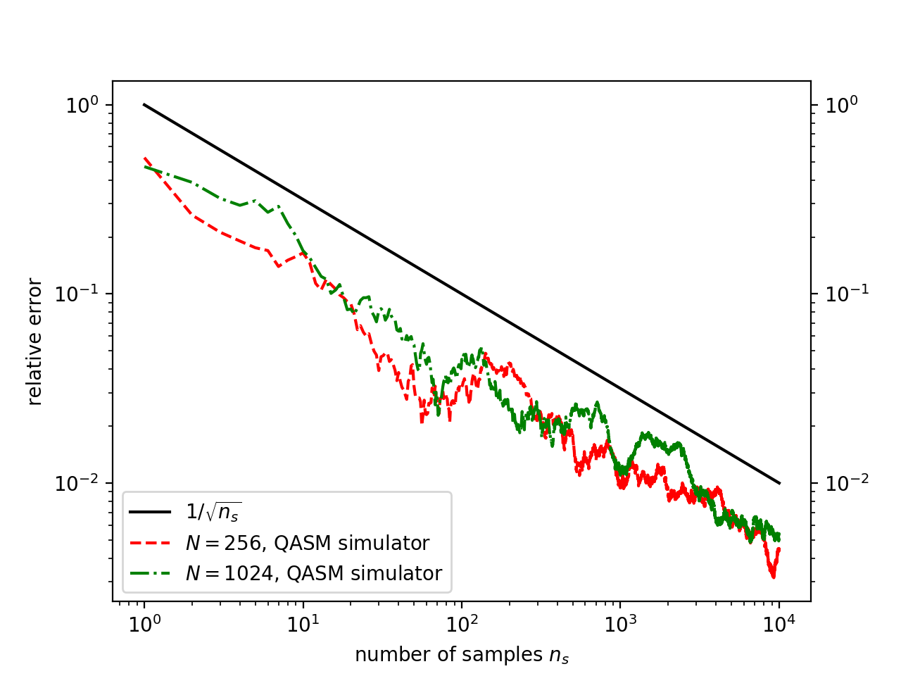
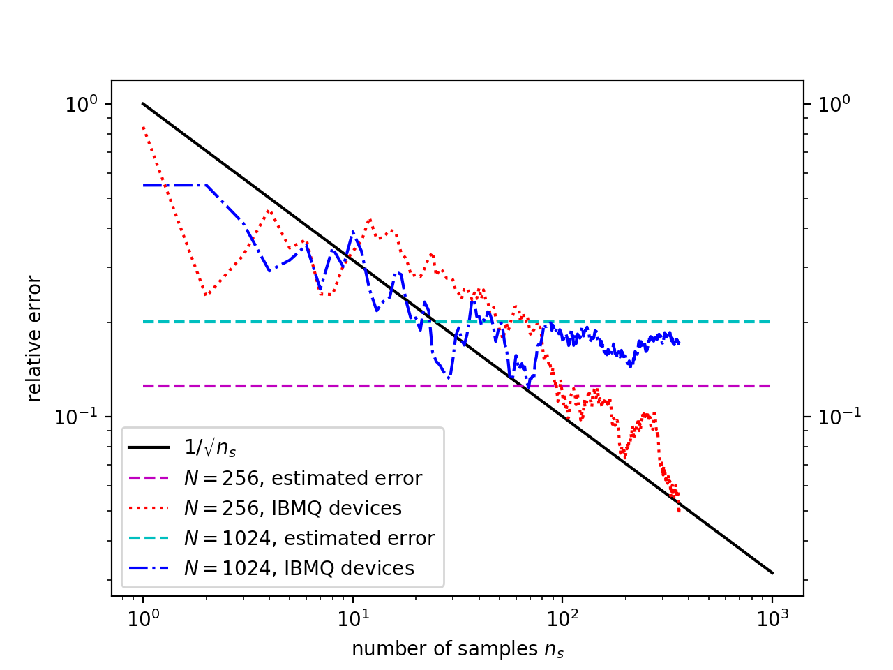
Figure 3: Relative errors $\epsilon=|x^{exact}_{I}-x_{I}|/|x^{exact}_{I}|$ as a function of the sampling number $n_{s}$ for $N=256$ and $N=1024$ matrices. The relevant parameters and estimated errors for these two matrices can be found in Table 1. Black solid lines represent the $1/\sqrt{n_{s}}$ error reduction expected for Monte Carlo calculations. (Upper figure) Red dashed line and green dash-dotted line are the results computed by the QASM simulator. (Lower figure) Blue dash-dotted line and red dotted line are data for the same matrices computed by the IBM Q 20 Tokyo machine or Poughkeepsie machine. Cyan and magenta horizontal dashed lines depict the estimated errors.

In comparison to Eq. (3) obtained from the classical random walk, we see that additional $\mathcal{O}(\log(N))$ XOR operations are required for classical computer to obtain the same quantum transition probability matrix, as can be seen from Eq. (II.3). In the case of $N=4$, the classical and quantum transition probability matrices given by Eqs. (4) and (10) are related by a permutation $\begin{pmatrix}0&1&2&3\\ 0&3&2&1\end{pmatrix}$. The quantum version of the Hamming distance between $|J\rangle_{q}$ and $|J^{\prime}\rangle_{q}$ is given by $d^{quantum}=\sum_{\ell=0}^{n-1}i_{\ell}\oplus i_{\ell-1}$, which clearly shows the temporal correlation between the $\ell$-th and $(\ell-1)$-th qubits. We attribute this correlation to the fact that only one quantum coin is used to decide on the Pauli $X$ gate over all the $n$ qubits, thus creating some connection between qubits, and to the non-Markovian nature of quantum walk dynamics Breuer et al. (2016); de Vega and Alonso (2017), in which the quantum circuit memorizes the qubit state $|i_{\ell-1}\rangle$ when it is walking in the direction that has the qubit state $|i_{\ell}\rangle$ in the Hamming cube.

It can be of interest to note that the circuit given in Eq. (6) is just one possible design leading to a particular correlation between qubits. In general, there are numerous ways to rearrange the walking steps to obtain different kinds of correlation, and it is possible to design the circuit for specific purposes. A simple way is to perform the walking steps in Eq. (6) in a reverse order, operating the $k=n-1$ operator to the right first, followed by the $k=n-2$ operator, and so on. This leads to a different metric $d^{quantum}=\sum_{\ell=0}^{n-1}i_{\ell+1}\oplus i_{\ell}$ with $i_{n}=0$. It turns out that this $d^{quantum}$ corresponds to the Hamming distance in the Gray code representation.

The Gray code uses single-distance coding for integer sequence $0\rightarrow 1\rightarrow\cdots\rightarrow N-1$, where adjacent integers differ by single bit flipping. In the case of the four-node graph in Fig. 1, the integers $(0,1,2,3)$ in the Gray code representation correspond to the $|00\rangle$, $|01\rangle$, $|11\rangle$, $|10\rangle$ states, respectively. It is obvious that this Gray code representation can be obtained from the natural binary code representation by a permutation $\begin{pmatrix}0&1&2&3\\ 0&1&3&2\end{pmatrix}$. There also exists a permutation that transforms $\textbf{P}^{classical}$ to $\textbf{P}^{quantum}$ in the Gray code basis. The proof of this correspondence for arbitrary $N$ is given in Appendix A. Both the transform and inverse transform between the natural binary code and Gray code representations take $\mathcal{O}(\log(N))$ operations using classical computer Knuth (2005). This again shows that the quantum random walk algorithm gains $\mathcal{O}(\log(N))$ improvement over the classical one.

Table 1: Relevant parameters for the matrices A of various sizes used for numerical experiments. Estimated error is defined in the text.

N	c	q	$\gamma$	Condition number	Estimated error $\epsilon_{0}$
64	6	2	0.3	1.457
128	6	2	0.3	1.599
256	6	1	0.3	1.857	0.1255
1024	10	1	0.5	2.973	0.2010

As the change of the Hamming distance for each walking step in the Gray code representation is $\delta d=1$, a quantum walker in a geodesic of a Hamming cube automatically walks with the least action, that is, with the minimum change of the Hamming distance. This geodesic is a Hamiltonian path on hypercubes Gilbert (1958).

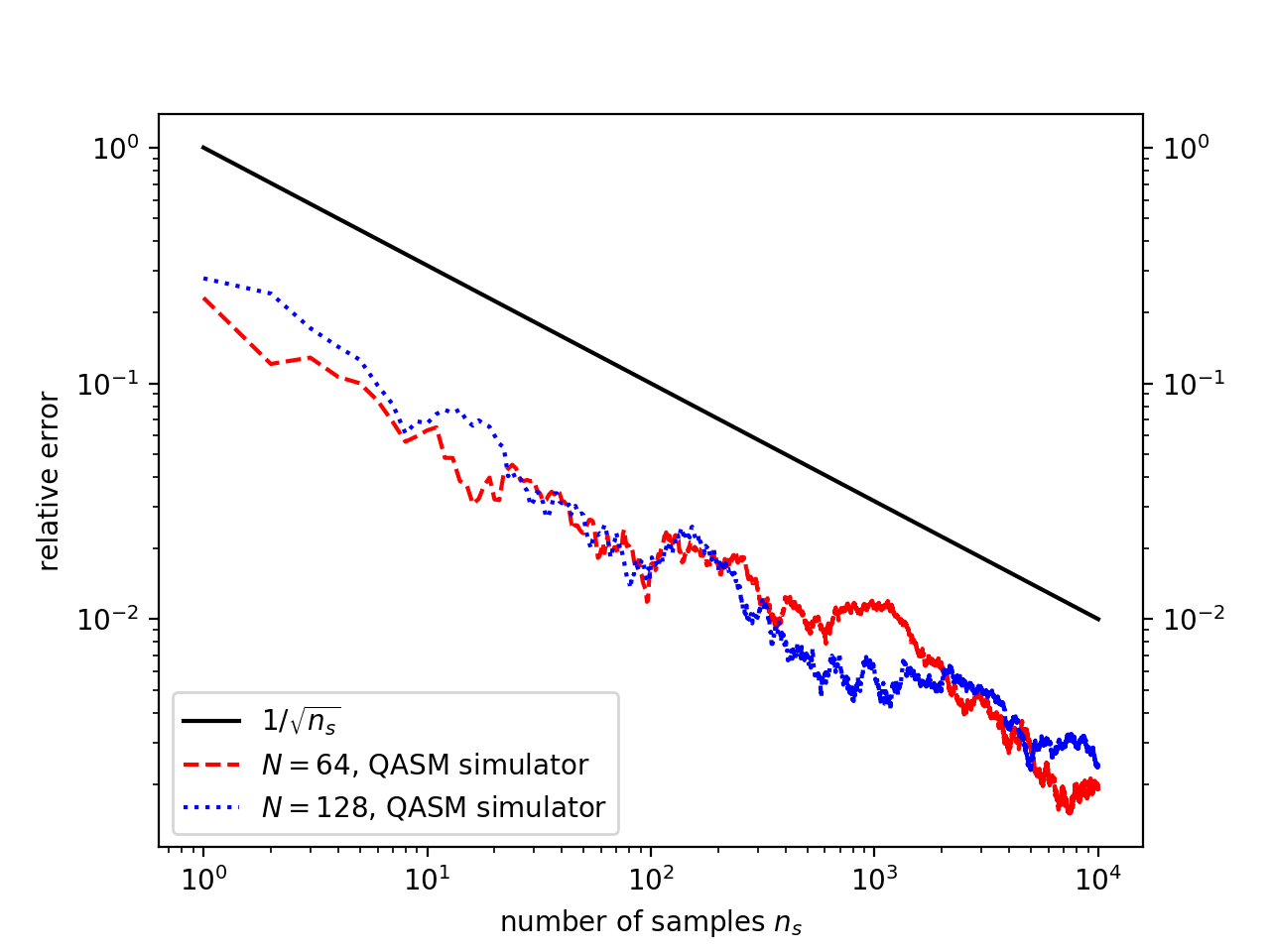
Figure 4: Relative errors $\epsilon=|x^{exact}_{I}-x_{I}|/|x^{exact}_{I}|$ as a function of the sampling number $n_{s}$ for $N=64$ and $N=128$ matrices, obtained by performing two quantum walk evolutions, $\mathcal{U}^{2}$. Black solid lines represent the $1/\sqrt{n_{s}}$ error reduction expected for Monte Carlo calculations. Red dashed line and blue dotted line are the results computed by the QASM simulator.

It is possible to increase the level of correlation in the probability matrix by performing multiple quantum evolutions, $\mathcal{U}^{q}$, where $q$ is the number of quantum walk evolutions. The probability matrix produced by two quantum walk evolutions, $\mathcal{U}^{2}$, is given by (see Appendix B for derivation)

$$P_{J^{\prime},J}^{quantum} = \sum_{k=0}^{1}\Big{|}\sum_{I}f(I,J^{\prime}\oplus J\oplus I)\delta_{i_{n-1},k}\Big{|}^{2}\,,$$ (11)

where, for $I=(i_{n-1},...,i_{0})$ and $K=(k_{n-1},...,k_{0})$,

$$f(I,K) = [U_{3}({\bf u}_{n-1})]_{i_{n-1},i_{n-2}}\cdots[U_{3}({\bf u}_{0})]_{i_{0},k_{n-1}}$$

$$\times[U_{3}({\bf u}_{n-1})]_{k_{n-1},k_{n-2}}\cdots[U_{3}({\bf u}_{0})]_{k_{0},0}\,,$$

and

$$[U_{3}(\theta,\phi,\lambda)]_{\mu,\nu}$$ (13)

$$=e^{i[\mu\phi+\nu\lambda]}(-1)^{(1-\mu)\nu}\Big{(}\cos(\frac{\theta}{2})\Big{)}^{1-(\mu\oplus\nu)}\Big{(}\sin(\frac{\theta}{2})\Big{)}^{\mu\oplus\nu}\,.$$

The fact that the summation over $I$ in Eq. (11) runs over $\mathcal{O}(2^{n})$ state configurations before the square is taken points to the complicated mixing of negative signs and complex phases $\phi_{\ell}$’s and $\lambda_{\ell}$’s. The sign problem makes it difficult for pure classical Monte Carlo methods to simulate this transition.

In general, the dependence of the two-evolution quantum probability matrix on $\theta_{\ell}$’s, $\phi_{\ell}$’s and $\lambda_{\ell}$’s, is not trivial. Its explicit expression for the $N=4$ graph is given in Appendix C. The phases $\phi_{\ell}$’s and $\lambda_{\ell}$’s enter into play for graph sizes $N\geq 8$. On the other hand, the two-evolution probability matrix for classical random walk is given by

$$P_{J^{\prime},J}^{classical}=$$ (14)

$$\prod_{\ell=0}^{n-1}\Big{|}\cos^{4}(\frac{\theta_{\ell}}{2})+\sin^{4}(\frac{\theta_{\ell}}{2})\Big{|}^{1-i_{\ell}}\Big{|}2\cos^{2}(\frac{\theta_{\ell}}{2})\sin^{2}(\frac{\theta_{\ell}}{2})\Big{|}^{i_{\ell}},$$

which is still factorisable.

Table 2: Comparison of various algorithms for solving $N\times N$ linear systems $\textbf{A}\vec{x}=\vec{b}$, with respect to time and space complexities, and Input/Output issues. Note that for classical Monte Carlo (MC) method, classical random walk (RW) and hybrid quantum random walk (QW), the time complexities in the table are per sampling time. It takes $\mathcal{O}(cn_{s})$ samplings to achieve the desired accuracy (see the text).

Algorithm	Time	Space for A	Input/Output
Classical DirectGolub and Van Loan (1996); Saad (2003)	$\mathcal{O}(N^{3})$	$\mathcal{O}(N^{2})$	efficient for any $\textbf{A},\vec{x},\vec{b}$
Classical IterativeGolub and Van Loan (1996); Saad (2003)	$\mathcal{O}(N^{2})$	$\mathcal{O}(N^{2})$	efficient for any $\textbf{A},\vec{x},\vec{b}$
Quantum HHLHarrow et al. (2009)	$\mathcal{O}(\log(N))$	$\mathcal{O}(\log(N))$ qubits	norm $||\vec{x}||$ not available
			difficult for $\textbf{A},\vec{x},\vec{b}$
Classical MCForsythe and Leibler (1950); Barto and Duff (1993); Lu and Schuurmans (2003)	$\mathcal{O}(N)$	$\mathcal{O}(N)$	efficient for any $\vec{x},\vec{b}$
(for one component $x_{I}$)			limited A (stochastic P)
Classical RW on HC	$\mathcal{O}(\log(N))$	$\mathcal{O}(\log(N))$	efficient for any $\vec{x},\vec{b}$
(for one component $x_{I}$)			limited A (factorisable P)
Hybrid QW on HC	$\mathcal{O}(\log(N))$	$\mathcal{O}(\log(N))$ qubits	efficient for any $\vec{x},\vec{b}$
(for one component $x_{I}$)			limited A (correlated P)

III Numerical results

Figure 3 shows the performance of our hybrid quantum random walk algorithm on linear systems of dimension $N=256$ and $N=1024$. Their relative errors decrease with increasing sampling number. The relative error is defined as $\epsilon=|x^{exact}_{I}-x_{I}|/|x^{exact}_{I}|$ for the $I$-th component of the solution vector $\vec{x}$, where $\vec{x}^{exact}$ is the exact result obtained with the NumPy package. To demonstrate, we use randomly generated vectors $\vec{b}$ and matrices A with a uniform distribution, $b_{I}\in[-1,1]$ and $\theta_{\ell}\in[0,\pi]$. We choose $\gamma$ and $c$ such that the error introduced by the Neumann expansion is within $\mathcal{O}(10^{-4})$. See Table 1 for the relevant parameters of the two matrices. The program is written and compiled with Qiskit version 0.7.2. The simulation results (upper figure) are obtained using QASM simulator Aleksandrowicz et al. (2019), while the quantum machine results (lower figure) are obtained using IBM Q 20 Tokyo device or Poughkeepsie device IBM (2019a, b).

The curves obtained by the QASM simulator are results averaged over ten runs. Their relative errors decrease as $1/\sqrt{n_{s}}$, where $n_{s}$ is the number of random walk samplings. This $1/\sqrt{n_{s}}$ reduction is typical of Monte Carlo simulations, because the hybrid quantum walk algorithm has essentially the same structure as classical Monte Carlo methods. So, we do not gain any speedup in sampling number. Yet, this result substantiates the fact that our proposed algorithm works on ideal quantum computers.

For real IBM Q quantum devices, the accuracy stops improving after a certain number of samplings (see the plateau (blue dash-dotted curve) and oscillation (red dotted curve) in Fig. 3). This hardware limitation can be estimated using an error formula $\epsilon_{0}\sim\kappa\times E_{r}$, where $\kappa$ is the condition number for the matrix A and $E_{r}$ is the readout error of real machines. The condition number $\kappa$ gauges the ratio of the relative error in the solution vector $\vec{x}$ to the relative error in the A matrix Saad (2003): some perturbation in the matrix, $\textbf{A}+\delta\textbf{A}$, can cause an error in the solution vector, $\vec{x}+\delta\vec{x}$, such that $||\delta\vec{x}||\sim\kappa\times||\delta\textbf{A}||$. By taking $E_{r}$ as an estimate for $||\delta\textbf{A}||$, we obtain the above error for the solution vector as $\epsilon_{0}=||\delta\vec{x}||\sim\kappa\times E_{r}$. The condition numbers given in Table 1 are computed by using Eq. (II.3) to construct the A matrices. For the average readout error of IBM Q 20 Tokyo device, we use $E_{r}=6.76\times 10^{-2}$ IBM (2019a). The estimated errors $\epsilon_{0}$ are given in Table 1. We see that the relative errors fall below the respective errors, indicating that the precision limit is due to the readout error of the current NISQ hardware. Note that the machines are calibrated several times during data collection, so the hardware error varies and the $E_{r}$ value is only an estimate.

Figure 4 shows the results for linear systems of dimension $N=64$ and $N=128$, obtained by the QASM simulator that performs two quantum walk evolutions with uniformly distributed $(\theta_{\ell},\phi_{\ell},\lambda_{\ell})\in[0,\pi]$. The relevant parameters for these two matrices are given in Table 1. The results again evidence that the algorithm works well, even in the presence of complex phases $\phi_{\ell}$’s and $\lambda_{\ell}$’s.

The communication latency between classical and quantum computer is the most time-consuming part, containing $\mathcal{O}(cn_{s})$ communications. Fortunately, this number does not scale as $N$. For users with direct access to the quantum processors, communication bottleneck should be less severe.

IV Discussions

A comparison of computational resources is given in Table 2. For hybrid quantum walk algorithm, we need $1+\log(N)$ qubits, $q\log(N)$ CNOT gates, and $q\log(N)$ $U_{3}$ gates, where $q$ is the number of evolutions. The initialization takes $\log(N)$ $X$ gates; but since they can be executed simultaneously, the initialization occupies one time slot only. Totally $1+2q\log(N)$ time slots are required for one quantum walk evolution to obtain one component of the solution vector $\vec{x}$. This can be an advantage when one is interested in partial information about $\vec{x}$.

The same amount of time slots can be similarly derived for the classical random walk algorithm. Yet, we stress that these two algorithms deal with different transition probability matrices: factorisable matrices for classical random walk, and more complex correlated matrices for quantum random walk. The qubit-qubit correlation built into the correlated matrix can potentially be harnessed to perform complex tasks.

Other advantages of the algorithms we propose are:

(i) By restricting the matrices A to those that can be encoded in Hamming cubes, we can sample both classical and quantum random walk spaces that scale exponentially with the number of bits/qubits, and hence gain space complexity.

(ii) Classical Monte Carlo methods have time complexity of $\mathcal{O}(N)$ for general P matrices. For the matrices here considered, our algorithms have $\mathcal{O}(\log(N))$.

(iii) It is easier to access input and output than the HHL-type algorithm.

(iv) Random processes in a quantum computer are fundamental, and so are not plagued by various problems associated with pseudo-random number generators Srinivasan et al. (2003), like periods and unwanted correlations.

(v) Our quantum algorithm can run on noisy quantum computers whose coherence time is short.

V Conclusion

We propose a hybrid quantum algorithm suitable for NISQ quantum computers to solve systems of linear equations. The solution vector $\vec{x}$ and constant vector $\vec{b}$ we consider here are classical data, so the input and readout can be executed easily. Numerical simulations using IBM Q systems support the feasibility of this algorithm. We demonstrate that, by performing two quantum walk evolutions, the resulting probability matrix become more correlated in the parameter space. As long as the quantum circuit in this framework produces highly correlated probability matrix with a relatively short circuit depth, we can always gain quantum advantages over classical circuits.

Appendix A Gray code basis

The natural binary code $B=(B_{n-1},B_{n-2},...,B_{1},B_{0})$ is transformed to the Gray code basis Knuth (2005) according to

$$g(B)_{i}=B_{i+1}\oplus B_{i},$$ (A.1)

$\forall i\in\{0,...,n-1\}$ with $B_{n}=0$. The probability matrix in the Gray code basis is given by

$$P^{quantum}_{J^{\prime},J} = \prod_{\ell=0}^{n-1}\Big{|}U_{3}(\theta_{\ell})_{i_{\ell},i_{\ell+1}}\Big{|}^{2}$$

$$= \prod_{\ell=0}^{n-1}\Big{|}\cos^{2}(\frac{\theta_{\ell}}{2})\Big{|}^{1-(i_{\ell}\oplus i_{\ell+1})}\Big{|}\sin^{2}(\frac{\theta_{\ell}}{2})\Big{|}^{i_{\ell}\oplus i_{\ell+1}}$$

with $i_{N}=0$.

Lemma 1.

Let $S_{N}$ be the set of all possible n-bit strings $\{(S_{n-1},S_{n-2},...,S_{1},S_{0})|S_{i}\in\{0,1\}~{}\forall~{}i\in\{0,1,...,n-1\}\}$ with $n=\log_{2}N$, and $\pi$ be a permutation of the set $S_{N}$. If there exists a function $f:S_{N}\mapsto\mathbb{R}$ such that for $A\in\mathbb{R}^{N\times N}$,

$$A_{I\oplus J,J}=f(I)$$ (A.3)

$\forall~{}I,J\in S_{N}$, and if $\pi$ is bitwise XOR homomorphic, then we have $A_{\pi(I\oplus J),\pi(J)}=f(\pi(I))$.

Proof.

Since $\pi$ is bitwise XOR homomorphic, Eq. (A.3) leads to

$$A_{\pi(I\oplus J),\pi(J)} = A_{\pi(I)\oplus\pi(J),\pi(J)}$$ (A.4)

$$= f(\pi(I))$$

$\forall~{}I,J\in S_{N}$. ∎

Lemma 2.

Let $B\in S_{N}$ be represented by $(B_{n-1},...,B_{0})$. Let $g:S_{N}\mapsto S_{N}$ be a function that transforms from natural bit string to Gray code according to $g(B)_{i}=B_{i+1}\oplus B_{i}$, $\forall~{}i\in\{0,1,...,n-1\}$ with $B_{n}=0$. Then $g$ is a bitwise XOR homomorphism.

Proof.

Let $I,J\in S_{N}$ be represented by bit strings $(I_{n-1},...,I_{0})$ and $(J_{n-1},...,J_{0})$, respectively. Using

$$g(I)_{i} = I_{i+1}\oplus I_{i}$$

$$g(J)_{i} = J_{i+1}\oplus J_{i}$$ (A.5)

with $I_{n}=J_{n}=0$, we get

$$[g(I)\oplus g(J)]_{i} = g(I)_{i}\oplus g(J)_{i}$$ (A.6)

$$= (I_{i+1}\oplus I_{i})\oplus(J_{i+1}\oplus J_{i})$$

$$= (I_{i+1}\oplus J_{i+1})\oplus(I_{i}\oplus J_{i})$$

$$= g(I\oplus J)_{i}.$$

$\forall~{}i\in{0,...,n-1}$. ∎

Using Lemma 1 and Lemma 2, the following theorem is clear.

Theorem 1.

There exists a permutation that maps the probability matrix produced by classical random walk to the probability matrix given in Eq. (A) produced by the quantum random walk circuit in a reverse order, that is, in Gray code basis.

Appendix B Derivation of Eq. (11)

We use the evolution operator given in Eq. (6),

$$\mathcal{U}=\!\!\!\!\sum_{i_{n-1},...,i_{0},i_{-1}}\prod_{\ell=0}^{n-1}[U_{3}({\bf u}_{\ell})]_{i_{\ell},i_{\ell-1}}(X_{\ell})^{i_{\ell}}(|i_{n-1}\rangle_{\diamond}\langle i_{-1}|_{\diamond})$$ (B.1)

to compute the two-evolution operator

$$\mathcal{U}^{2}\!\!\! = \!\!\!\sum_{\begin{subarray}{c}i_{n-1},...,i_{0},i_{-1}\\ k_{n-1},...,k_{0},k_{-1}\end{subarray}}\prod_{\ell=0}^{n-1}[U_{3}({\bf u}_{\ell})]_{i_{\ell},i_{\ell-1}}[U_{3}({\bf u}_{\ell})]_{k_{\ell},k_{\ell-1}}$$ (B.2)

$$\times(X_{\ell})^{i_{\ell}+k_{\ell}}\delta_{i_{-1},k_{n-1}}(|i_{n-1}\rangle_{\diamond}\langle k_{-1}|_{\diamond})\,.$$

Next we project the $\mathcal{U}^{2}$ operator on the $|\psi_{0J}\rangle$ state,

$$\mathcal{U}^{2}|\psi_{0J}\rangle = \sum_{\begin{subarray}{c}i_{n-1},...,i_{0},i_{-1}\\ k_{n-1},...,k_{0},k_{-1}\end{subarray}}\prod_{\ell=0}^{n-1}[U_{3}({\bf u}_{\ell})]_{i_{\ell},i_{\ell-1}}[U_{3}({\bf u}_{\ell})]_{k_{\ell},k_{\ell-1}}$$ (B.3)

$$\times\delta_{i_{-1},k_{n-1}}\delta_{0,k_{-1}}|i_{n-1}\rangle_{\diamond}|I\oplus K\oplus J\rangle_{q}$$

$$= \sum_{I,K}f(I,K)|i_{n-1}\rangle_{\diamond}|I\oplus K\oplus J\rangle_{q}\,,$$

where $f(I,K)$ is given in Eq. (II.3) and

$$|I\oplus K\oplus J\rangle_{q}=|i_{n-1}\oplus k_{n-1}\oplus j_{n-1},...,i_{0}\oplus k_{0}\oplus j_{0}\rangle_{q}\,.$$

We then project $\mathcal{U}^{2}|\psi_{0J}\rangle$ on the final state $|k\rangle_{\diamond}|J^{\prime}\rangle_{q}$

$$\langle J^{\prime}|_{q}\langle k|_{\diamond}\mathcal{U}^{2}|\psi_{0J}\rangle = \sum_{I,K}f(I,K)\delta_{k,i_{n-1}}\delta_{J^{\prime},I\oplus K\oplus J}$$ (B.4)

$$= \sum_{I}f(I,I\oplus J^{\prime}\oplus J)\delta_{k,i_{n-1}},$$

which leads to the probability matrix elements as

$$P_{J^{\prime},J} =\langle J^{\prime}|\mbox{Tr}_{\diamond}[\mathcal{U}^{2}|\psi_{0J}\rangle\langle\psi_{0J}|(\mathcal{U}^{\dagger})^{2}]|J^{\prime}\rangle$$ (B.5)

$$=\sum_{k}\Big{|}\langle J^{\prime}|_{q}\langle k|_{\diamond}\mathcal{U}^{2}|\psi_{0J}\rangle\Big{|}^{2}$$

$$=\sum_{k=0}^{1}\Big{|}\sum_{I}f(I,J^{\prime}\oplus J\oplus I)\delta_{i_{n-1},k}\Big{|}^{2}.$$

Appendix C Two-evolution quantum walk on $N=4$ graph

The probability matrix elements $P^{quantum}_{J^{\prime},J}$ for two quantum evolutions $\mathcal{U}^{2}$ on the four-node graph read

$$P_{00} = P_{11}=P_{22}=P_{33}$$

$$= \frac{1}{4}\sin^{2}\theta_{0}+\frac{1}{8}(1+\cos^{2}\theta_{1}+\cos^{2}\theta_{0}$$

$$+4\cos\theta_{1}\cos\theta_{0}+\cos^{2}\theta_{1}\cos^{2}\theta_{0}-\sin^{2}\theta_{1}\sin^{2}\theta_{0}),$$

$$P_{01} = P_{23}=\frac{1}{4}\sin^{2}\theta_{1},$$ (C.2)

$$P_{02} = P_{13}=\frac{1}{4}\sin^{2}\theta_{1},$$ (C.3)

$$P_{03} = P_{12}=\frac{1}{4}\Big{(}1-2\cos\theta_{1}\cos\theta_{0}+\cos^{2}\theta_{1}\Big{)}\,.$$ (C.4)

Surprisingly, in this case the matrix elements do not depend on the $(\phi_{1},\phi_{2})$ and $(\lambda_{1},\lambda_{2})$ phases. However, the matrix elements do depend on complex phases when $N\geq 8$, as can be numerically checked. Note that $(P_{01},P_{02},P_{23},P_{13})$ depend on $\theta_{1}$ only: the destructive interference between configurations totally eliminates the $\theta_{0}$ dependence, which is difficult to do by simple classical random walks.

References

- Nielsen and Chuang (2011) M. A. Nielsen and I. L. Chuang, Quantum Computation and Quantum Information: 10th Anniversary Edition (Cambridge University Press, New York, NY, USA, 2011), 10th ed., ISBN 1107002176, 9781107002173.
- Golub and Van Loan (1996) G. H. Golub and C. F. Van Loan, Matrix Computations (3rd Ed.) (Johns Hopkins University Press, Baltimore, MD, USA, 1996), ISBN 0-8018-5414-8.
- Saad (2003) Y. Saad, Iterative Methods for Sparse Linear Systems (Society for Industrial and Applied Mathematics, Philadelphia, PA, USA, 2003), 2nd ed., ISBN 0898715342.
- Harrow et al. (2009) A. W. Harrow, A. Hassidim, and S. Lloyd, Phys. Rev. Lett. 103, 150502 (2009), URL https://link.aps.org/doi/10.1103/PhysRevLett.103.150502.
- Clader et al. (2013) B. D. Clader, B. C. Jacobs, and C. R. Sprouse, Phys. Rev. Lett. 110, 250504 (2013), URL https://link.aps.org/doi/10.1103/PhysRevLett.110.250504.
- Montanaro and Pallister (2016) A. Montanaro and S. Pallister, Phys. Rev. A 93, 032324 (2016), URL https://link.aps.org/doi/10.1103/PhysRevA.93.032324.
- Childs et al. (2017) A. Childs, R. Kothari, and R. Somma, SIAM Journal on Computing 46, 1920 (2017), eprint https://doi.org/10.1137/16M1087072, URL https://doi.org/10.1137/16M1087072.
- Costa et al. (2019) P. C. S. Costa, S. Jordan, and A. Ostrander, Phys. Rev. A 99, 012323 (2019), URL https://link.aps.org/doi/10.1103/PhysRevA.99.012323.
- Berry et al. (2017) D. W. Berry, A. M. Childs, A. Ostrander, and G. Wang, Communications in Mathematical Physics 356, 1057 (2017), ISSN 1432-0916, URL https://doi.org/10.1007/s00220-017-3002-y.
- Dervovic et al. (2018) D. Dervovic, M. Herbster, P. Mountney, S. Severini, N. Usher, and L. Wossnig, arXiv e-prints arXiv:1802.08227 (2018), eprint 1802.08227.
- Wossnig et al. (2018) L. Wossnig, Z. Zhao, and A. Prakash, Phys. Rev. Lett. 120, 050502 (2018), URL https://link.aps.org/doi/10.1103/PhysRevLett.120.050502.
- Biamonte et al. (2017) J. Biamonte, P. Wittek, N. Pancotti, P. Rebentrost, N. Wiebe, and S. Lloyd, Nature (London) 549, 195 (2017), eprint 1611.09347.
- Ciliberto et al. (2018) C. Ciliberto, M. Herbster, A. D. Ialongo, M. Pontil, A. Rocchetto, S. Severini, and L. Wossnig, Proceedings of the Royal Society of London Series A 474, 20170551 (2018), eprint 1707.08561.
- Deutsch (1985) D. Deutsch, Proceedings of the Royal Society of London. A. Mathematical and Physical Sciences 400, 97 (1985).
- Kadowaki and Nishimori (1998) T. Kadowaki and H. Nishimori, Phys. Rev. E 58, 5355 (1998), URL https://link.aps.org/doi/10.1103/PhysRevE.58.5355.
- Farhi et al. (2000) E. Farhi, J. Goldstone, S. Gutmann, and M. Sipser, eprint arXiv:quant-ph/0001106 (2000), eprint quant-ph/0001106.
- Aharonov et al. (2008) D. Aharonov, W. van Dam, J. Kempe, Z. Landau, S. Lloyd, and O. Regev, SIAM Review 50, 755 (2008), eprint https://doi.org/10.1137/080734479, URL https://doi.org/10.1137/080734479.
- O’Malley and Vesselinov (2016) D. O’Malley and V. V. Vesselinov, in 2016 IEEE High Performance Extreme Computing Conference (HPEC) (2016), pp. 1–7.
- Borle and Lomonaco (2018) A. Borle and S. J. Lomonaco, arXiv e-prints arXiv:1809.07649 (2018), eprint 1809.07649.
- Chang et al. (2018) C. C. Chang, A. Gambhir, T. S. Humble, and S. Sota, arXiv e-prints arXiv:1812.06917 (2018), eprint 1812.06917.
- Wen et al. (2019) J. Wen, X. Kong, S. Wei, B. Wang, T. Xin, and G. Long, Phys. Rev. A 99, 012320 (2019), URL https://link.aps.org/doi/10.1103/PhysRevA.99.012320.
- Subaş ı et al. (2019) Y. b. u. Subaş ı, R. D. Somma, and D. Orsucci, Phys. Rev. Lett. 122, 060504 (2019), URL https://link.aps.org/doi/10.1103/PhysRevLett.122.060504.
- Preskill (2018) J. Preskill, Quantum 2, 79 (2018), ISSN 2521-327X, URL https://doi.org/10.22331/q-2018-08-06-79.
- Cao et al. (2012) Y. Cao, A. Daskin, S. Frankel, and S. Kais, Molecular Physics 110, 1675 (2012), eprint https://doi.org/10.1080/00268976.2012.668289, URL https://doi.org/10.1080/00268976.2012.668289.
- Cai et al. (2013) X.-D. Cai, C. Weedbrook, Z.-E. Su, M.-C. Chen, M. Gu, M.-J. Zhu, L. Li, N.-L. Liu, C.-Y. Lu, and J.-W. Pan, Phys. Rev. Lett. 110, 230501 (2013), URL https://link.aps.org/doi/10.1103/PhysRevLett.110.230501.
- Barz et al. (2014) S. Barz, I. Kassal, M. Ringbauer, Y. O. Lipp, B. Dakić, A. Aspuru-Guzik, and P. Walther, Scientific Reports 4, 6115 (2014), eprint 1302.1210.
- Pan et al. (2014) J. Pan, Y. Cao, X. Yao, Z. Li, C. Ju, H. Chen, X. Peng, S. Kais, and J. Du, Phys. Rev. A 89, 022313 (2014), URL https://link.aps.org/doi/10.1103/PhysRevA.89.022313.
- Zheng et al. (2017) Y. Zheng, C. Song, M.-C. Chen, B. Xia, W. Liu, Q. Guo, L. Zhang, D. Xu, H. Deng, K. Huang, et al., Phys. Rev. Lett. 118, 210504 (2017), URL https://link.aps.org/doi/10.1103/PhysRevLett.118.210504.
- Lee et al. (2019) Y. Lee, J. Joo, and S. Lee, Scientific reports 9, 4778 (2019).
- Aaronson (2015) S. Aaronson, Nature Physics 11, 291 (2015).
- Childs (2009) A. M. Childs, Nature Physics 5, 861 (2009).
- Möttönen et al. (2004) M. Möttönen, J. J. Vartiainen, V. Bergholm, and M. M. Salomaa, Phys. Rev. Lett. 93, 130502 (2004), URL https://link.aps.org/doi/10.1103/PhysRevLett.93.130502.
- Plesch and Brukner (2011) M. Plesch and i. c. v. Brukner, Phys. Rev. A 83, 032302 (2011), URL https://link.aps.org/doi/10.1103/PhysRevA.83.032302.
- Coles et al. (2018) P. J. Coles, S. Eidenbenz, S. Pakin, A. Adedoyin, J. Ambrosiano, P. Anisimov, W. Casper, G. Chennupati, C. Coffrin, H. Djidjev, et al., arXiv e-prints arXiv:1804.03719 (2018), eprint 1804.03719.
- James et al. (2001) D. F. V. James, P. G. Kwiat, W. J. Munro, and A. G. White, Phys. Rev. A 64, 052312 (2001), URL https://link.aps.org/doi/10.1103/PhysRevA.64.052312.
- Suess et al. (2017) D. Suess, Ł. Rudnicki, T. O. maciel, and D. Gross, New Journal of Physics 19, 093013 (2017), URL https://doi.org/10.1088%2F1367-2630%2Faa7ce9.
- Cramer et al. (2010) M. Cramer, M. B. Plenio, S. T. Flammia, R. Somma, D. Gross, S. D. Bartlett, O. Landon-Cardinal, D. Poulin, and Y.-K. Liu, Nature Communications 1, 149 (2010), eprint 1101.4366.
- Peruzzo et al. (2014) A. Peruzzo, J. McClean, P. Shadbolt, M.-H. Yung, X.-Q. Zhou, P. J. Love, A. Aspuru-Guzik, and J. L. O’Brien, Nature Communications 5, 4213 (2014), eprint 1304.3061.
- Wecker et al. (2015) D. Wecker, M. B. Hastings, and M. Troyer, Phys. Rev. A 92, 042303 (2015), URL https://link.aps.org/doi/10.1103/PhysRevA.92.042303.
- McClean et al. (2016) J. R. McClean, J. Romero, R. Babbush, and A. Aspuru-Guzik, New Journal of Physics 18, 023023 (2016), eprint 1509.04279.
- Kandala et al. (2017) A. Kandala, A. Mezzacapo, K. Temme, M. Takita, M. Brink, J. M. Chow, and J. M. Gambetta, Nature (London) 549, 242 (2017), eprint 1704.05018.
- Sutton and Barto (1998) R. S. Sutton and A. G. Barto, Introduction to Reinforcement Learning (MIT Press, Cambridge, MA, USA, 1998), 1st ed., ISBN 0262193981.
- Aleksandrowicz et al. (2019) G. Aleksandrowicz, T. Alexander, P. Barkoutsos, L. Bello, Y. Ben-Haim, D. Bucher, F. J. Cabrera-Hernádez, J. Carballo-Franquis, A. Chen, C.-F. Chen, et al., Qiskit: An open-source framework for quantum computing (2019).
- IBM (2016) IBM Q Experience, https://quantumexperience.ng.bluemix.net (2016), accessed: 12/01/2018.
- Barto and Duff (1993) A. Barto and M. Duff, in Proceedings of the 6th International Conference on Neural Information Processing Systems (Morgan Kaufmann Publishers Inc., San Francisco, CA, USA, 1993), NIPS’93, pp. 687–694, URL http://dl.acm.org/citation.cfm?id=2987189.2987276.
- Paparo et al. (2014) G. D. Paparo, V. Dunjko, A. Makmal, M. A. Martin-Delgado, and H. J. Briegel, Phys. Rev. X 4, 031002 (2014), URL https://link.aps.org/doi/10.1103/PhysRevX.4.031002.
- Goral et al. (1984) C. M. Goral, K. E. Torrance, D. P. Greenberg, and B. Battaile, SIGGRAPH Comput. Graph. 18, 213 (1984), ISSN 0097-8930, URL http://doi.acm.org/10.1145/964965.808601.
- Bravyi et al. (2008) S. Bravyi, D. P. Divincenzo, R. Oliveira, and B. M. Terhal, Quantum Info. Comput. 8, 361 (2008), ISSN 1533-7146, URL http://dl.acm.org/citation.cfm?id=2011772.2011773.
- Bravyi (2015) S. Bravyi, Quantum Info. Comput. 15, 1122 (2015), ISSN 1533-7146, URL http://dl.acm.org/citation.cfm?id=2871363.2871366.
- Metropolis and Ulam (1949) N. Metropolis and S. Ulam, Journal of the American Statistical Association 44, 335 (1949), pMID: 18139350, URL https://www.tandfonline.com/doi/abs/10.1080/01621459.1949.10483310.
- Forsythe and Leibler (1950) G. E. Forsythe and R. A. Leibler, Mathematics of Computation 4, 127 (1950).
- Wasow (1952) W. R. Wasow, Mathematical Tables and Other Aids to Computation 6, 78 (1952), ISSN 08916837, URL http://www.jstor.org/stable/2002546.
- Lu and Schuurmans (2003) F. Lu and D. Schuurmans, in Proceedings of the Nineteenth Conference on Uncertainty in Artificial Intelligence (Morgan Kaufmann Publishers Inc., San Francisco, CA, USA, 2003), UAI’03, pp. 386–393, ISBN 0-127-05664-5, URL http://dl.acm.org/citation.cfm?id=2100584.2100631.
- Branford et al. (2008) S. Branford, C. Sahin, A. Thandavan, C. Weihrauch, V. Alexandrov, and I. Dimov, Future Generation Computer Systems 24, 605 (2008), ISSN 0167-739X, URL http://www.sciencedirect.com/science/article/pii/S0167739X0700129X.
- Ceperley and Alder (1980) D. M. Ceperley and B. J. Alder, Phys. Rev. Lett. 45, 566 (1980), URL https://link.aps.org/doi/10.1103/PhysRevLett.45.566.
- Negele and Orland (1988) J. W. Negele and H. Orland, Quantum many-particle physics (Addison-Wesley, 1988).
- Landau and Binder (2005) D. Landau and K. Binder, A Guide to Monte Carlo Simulations in Statistical Physics (Cambridge University Press, New York, NY, USA, 2005), ISBN 0521842387.
- Hamming (1950) R. W. Hamming, The Bell System Technical Journal 29, 147 (1950), ISSN 0005-8580.
- Aharonov et al. (1993) Y. Aharonov, L. Davidovich, and N. Zagury, Phys. Rev. A 48, 1687 (1993), URL https://link.aps.org/doi/10.1103/PhysRevA.48.1687.
- Childs et al. (2001) A. M. Childs, E. Farhi, and S. Gutmann, eprint arXiv:quant-ph/0103020 (2001), eprint quant-ph/0103020.
- Aharonov et al. (2001) D. Aharonov, A. Ambainis, J. Kempe, and U. Vazirani, in Proceedings of the Thirty-third Annual ACM Symposium on Theory of Computing (ACM, New York, NY, USA, 2001), STOC ’01, pp. 50–59, ISBN 1-58113-349-9, URL http://doi.acm.org/10.1145/380752.380758.
- Moore and Russell (2002) C. Moore and A. Russell, in Randomization and Approximation Techniques in Computer Science, edited by J. D. P. Rolim and S. Vadhan (Springer Berlin Heidelberg, Berlin, Heidelberg, 2002), pp. 164–178, ISBN 978-3-540-45726-8.
- Szegedy (2004) M. Szegedy, in Proceedings of the 45th Annual IEEE Symposium on Foundations of Computer Science (IEEE Computer Society, Washington, DC, USA, 2004), FOCS ’04, pp. 32–41, ISBN 0-7695-2228-9, URL http://dx.doi.org/10.1109/FOCS.2004.53.
- Kendon (2006) V. M. Kendon, Philosophical Transactions of the Royal Society of London Series A 364, 3407 (2006), eprint quant-ph/0609035.
- Childs (2017) A. Childs, Lecture notes on quantum algorithms (2017).
- Košík and Bužek (2005) J. Košík and V. Bužek, Phys. Rev. A 71, 012306 (2005), URL https://link.aps.org/doi/10.1103/PhysRevA.71.012306.
- Shikano and Katsura (2010) Y. Shikano and H. Katsura, Phys. Rev. E 82, 031122 (2010), URL https://link.aps.org/doi/10.1103/PhysRevE.82.031122.
- Breuer et al. (2016) H.-P. Breuer, E.-M. Laine, J. Piilo, and B. Vacchini, Rev. Mod. Phys. 88, 021002 (2016), URL https://link.aps.org/doi/10.1103/RevModPhys.88.021002.
- de Vega and Alonso (2017) I. de Vega and D. Alonso, Rev. Mod. Phys. 89, 015001 (2017), URL https://link.aps.org/doi/10.1103/RevModPhys.89.015001.
- Knuth (2005) D. E. Knuth, The Art of Computer Programming, Volume 4, Fascicle 2: Generating All Tuples and Permutations (Art of Computer Programming) (Addison-Wesley Professional, 2005), ISBN 0201853930.
- Gilbert (1958) E. N. Gilbert, The Bell System Technical Journal 37, 815 (1958), ISSN 0005-8580.
- IBM (2019a) IBM Q devices and simulators, https://www.research.ibm.com/ibm-q/technology/devices/ (2019a), accessed: 2019-02-20.
- IBM (2019b) Cramming More Power Into a Quantum Device, https://www.ibm.com/blogs/research/2019/03/power-quantum-device/ (2019b), accessed: 2019-03-21.
- Srinivasan et al. (2003) A. Srinivasan, M. Mascagni, and D. Ceperley, Parallel Computing 29, 69 (2003), ISSN 0167-8191, URL http://www.sciencedirect.com/science/article/pii/S0167819102001631.