Superfluid Vortex Dynamics on Planar Sectors and Cones
Abstract
We study the dynamics of vortices formed in a superfluid film adsorbed on the curved two-dimensional surface of a cone. To this aim, we observe that a cone can be unrolled to a sector on a plane with periodic boundary conditions on the straight sides. The sector can then be mapped conformally to the whole plane, leading to the relevant stream function. In this way, we show that a superfluid vortex on the cone precesses uniformly at fixed distance from the apex. The stream function also yields directly the interaction energy of two vortices on the cone. We then study the vortex dynamics on unbounded and bounded cones. In suitable limits, we recover the known results for dynamics on cylinders and planar annuli.
I Introduction
Vortex dynamics in superfluid films depends strongly on the shape of the underlying surface. For example, a region with local positive Gaussian curvature (such as the top of a smooth hill, or the bottom of a valley) exerts a repulsive force on a vortex Vite04 ; Turn10 . Geometries with vanishing Gaussian curvature also have special features: for example, single vortices on an infinite cylinder have quantized azimuthal velocities Guen17 because of the single-valued nature of the condensate wave function. Here, we study the different and interesting case of superfluid vortex dynamics on a conical surface, which is equivalent to the motion on a planar sector Schi16 .
We consider a sector (a wedge) of the plane with opening angle , where is real and larger than one. We also impose periodic boundary conditions on the two radial sides. To determine the hydrodynamic flow arising from a singly quantized vortex at some complex position in the sector, we use the conformal transformation from the sector to the whole plane. Reference Schi16 considered the special case , but this transformation holds for general Rile06 . Note that the limiting case represents the whole plane.
Section II provides basic background for this problem, including the complex potential and the self-induced motion associated with the curved surface of the cone. The next Secs. III and IV consider the energy and dynamics of a system of vortices, where the interaction energy can be expressed simply in terms of the stream function. Section V generalizes to the case of bounded cones, both internally and externally. The last Sec. VI concludes with discussion and a brief conjecture about the situation for .
II Vortices on sectors and cones
We start from the full plane with complex coordinate . A fundamental tool for the description of hydrodynamics of two-dimensional incompressible and irrotational fluids is the complex potential , where is the stream function and is the velocity potential. Either function provides the hydrodynamic flow pattern with the general relation , with the mass of the superfluid particles. For a singly quantized positive vortex at , the complex potential is
| (1) |
and we use a conformal map to obtain the corresponding complex potential on the sector and the cone.
II.1 Geometry of cones and sectors
It is clear from elementary considerations that a finite cone (like a “dunce cap” or a “witch hat”) may be unrolled onto a wedge-shaped sector. Similarly, an infinite cone may be unfolded onto an infinite sector of the plane, or a truncated cone unfolds to a portion of an annulus. This procedure does not introduce any distortion, and therefore preserves both lengths and areas. It is also conformal, since it preserves angles locally.
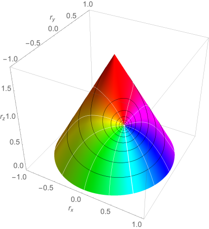
Let us here briefly review the geometric descriptions of a cone, and of the corresponding sector. The usual spherical polar coordinates () can make this connection precise, since an unbounded cone is the axisymmetric surface associated with fixed polar angle , leaving and as the two parameters specifying locations on the surface. In general, the three-dimensional coordinate vector becomes
| (2) |
expressed in spherical polar coordinates. The partial derivatives , , and yield (after normalization) the three orthogonal unit vectors , , and (see, for example Sec. 10.9.2 in Ref. Rile06 ). On the surface of the cone, the outward unit normal is with .
The apex angle of the cone is for and for , and the perpendicular distance from the symmetry axis to the conical surface is . Let or, equivalently , both with . Hence the perpendicular distance becomes , and . An illustrative sketch of the geometry under consideration is given in Fig. 1.
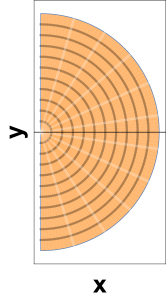
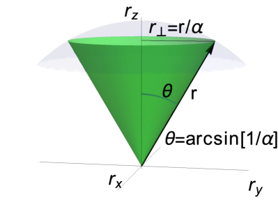
On the surface of the cone, the element of distance is . Introducing the parameter , which has the range , the element of distance becomes , which can now be treated as the element of distance on an unbounded planar sector (or wedge) of angular opening . In this way, we have a direct mapping from the surface of the cone with spherical polar coordinates and fixed to the planar sector with plane polar coordinates and wedge angle . Evidently, the same planar sector can yield a cone with apex that points up or down, depending on whether the surface of the sector appears on the outside or inside of the cone.
Note the two important limiting cases:
-
1.
If , then and . Here the cone becomes narrow and approaches a cylinder with open end pointing down or up, respectively (see below for more detailed discussion).
-
2.
If , then and . Here the cone becomes flat and the sector approaches the full plane.
For any , the cone has a sharp apex where the curvature is singular; this singularity disappears only for the special value or equivalently . On the smooth conical surface, the curvature vanishes along the radial direction and the curvature along the azimuthal direction is . Hence the Gaussian curvature vanishes but the mean curvature is generally nonzero. These results follow from the material in Secs. IV and V of Ref. Kami02 .
II.2 Conformal map, complex potential and vortex dynamics
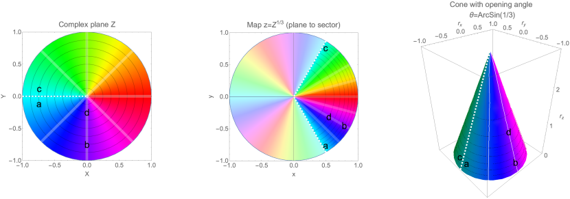
In this way, the behavior of a quantized vortex on the surface of a cone becomes equivalent to that of a two-dimensional vortex on a planar sector with opening angle and periodic boundary conditions on the two straight sides. Similar to the case of a cylinder and its equivalent infinite planar strip with periodic boundary conditions (see Refs. Ho15 ; Guen17 , and Appendix A), the conformal transformation
| (3) |
maps the whole plane with to the unbounded sector with . Hence we have , where and (for an application to electrostatics, see Sec. 25.2 in Ref. Rile06 ). The action of this map is illustrated in Fig. 2. Notice that for complex numbers the power function is defined through the logarithm function, , so that a choice of branch cut of the logarithm different from the principal one will result in a different angular range for the variable .
On the infinite plane, the complex potential for a positive singly quantized vortex at position is simply given by Eq. (1). The conformal transformation immediately gives the equivalent result for a positive vortex on an unbounded sector with apex angle :
| (4) |
Note that for (an integer), this result is simply the sum of contributions for the original vortex and its images equally spaced on a circle of radius . In terms of the variables on the cone, the corresponding stream function reads
| (5) |
For a general that includes multiple vortices and perhaps boundaries, it is not hard to show that the motion of a positive vortex at is
| (6) |
where the last term subtracts the (singular) circulating flow from the vortex itself. Given the complex potential in Eq. (4) for an unbounded sector (and hence for the surface of an infinite cone), an elementary calculation gives the result
| (7) |
or, equivalently, in vector form,
| (8) |
where and . If , the vortex becomes stationary, as expected because the sector then covers the whole plane and the equivalent cone becomes flat.
Note that the motion is purely azimuthal, so that the time taken to complete one cycle on the sector is
The frequency of the cyclic vortex motion around the cone is , and correspondingly the angular frequency around the cone is
| (9) |
expressed in terms of the radial distance along the surface from the apex of the cone. For many purposes, the more relevant distance is , yielding
| (10) |
In the limit , the apex angle becomes small, and the cone locally approaches a cylinder. In this limit Eq. (10) correctly reduces to the quantized result that we found for an infinite cylinder of radius in Ref. Guen17 .
It is also instructive to examine the limiting behavior for of the conformal transformation from a planar sector to the whole plane. Specifically, we now show that this transformation locally becomes that for the conformal transformation from a strip with periodic boundary conditions to the whole plane, which is discussed in detail in Appendix A. Indeed, consider a point on the sector with . Let with and . Here . The rescaling then gives the desired result . This mapping naturally associates the angle on the sector with the angle on the cylinder.
Finally, let us take a close look at the local flow around a vortex core located at . The stream function Eq. (5) may be expanded by introducing and , to obtain
| (11) |
which shows explicitly that, very close to the vortex core, the stream function is constant for circles defined by the constant squared distance . This result is expected, since vortex cores on the plane are circular, and conformal transformations preserve the shapes of infinitesimal objects. Circular streamlines are indeed visible in the vicinity of the cores in both Figs. 5 and 6.
III Energy of two vortices
In the present hydrodynamic model, the total energy of two vortices on a cone is purely kinetic:
| (12) |
where is the two-dimensional number density and is the total velocity. Here, with , and the charge of vortex . The total energy may be written as , where is the interaction energy between the two vortices, and and are the corresponding self-energies.
III.1 Interaction energy
The two cross terms in yield the interaction energy of two vortices
| (13) |
Use the two-dimensional divergence theorem to rewrite the integral as
| (14) |
where is the outward unit normal in the surface to the various boundaries. The second term immediately gives because .
The first term of Eq. (14) is a line integral around the boundary of the cone. It is natural to take two circles: one at radial distance since the apex of the cone is a singular region, and the other at because the overall integral is log divergent.
For small , the unit normal vector is . The relevant derivative becomes . The circumference is , so that this contribution vanishes for (note that this line integral also vanishes because of the cos factor).
On the large circle the stream function becomes so that . Here the unit vector is simply and the circumference is , so that this term contributes . Consequently, we find
| (15) |
where . Note that the argument of the logarithm is dimensionless, as it must be. This function is periodic in the relative angular displacement , but the dependence on the radial position () is more complicated, with the power laws involving the parameter . This behavior reflects the loss of translation symmetry along the radial axis of the cone because the cone’s tip serves as the origin of the spherical polar coordinates () with fixed .
III.2 Self-energy
Despite the loss of translational symmetry, the self-energy for a single vortex at position on a large cone of radial dimension is scarcely more intricate than for a plane or a cylinder. As for the interaction energy, we again integrate by parts
| (16) |
where the integral is over the surface of the bounded cone with excluding a small circle of radius around the vortex core (and a small circle around the apex of the cone, which is irrelevant here). This exclusion near the vortex means that the second term in Eq. (16) never contributes. In addition, the first term can be evaluated readily with the two-dimensional divergence theorem
| (17) |
where the integral is over all boundaries on the surface and is the outward unit normal in the surface to the boundaries of the original area (here the large circle at and the small circle around the vortex core).
Start with the large circle at , where is just the unit vector . For , the stream function (5) simplifies to , and a straightforward calculation gives the contribution .
Next, consider the small circle around the vortex core, where Eq. (11) shows that the flow is axisymmetric around the vortex. Define so that a local radial variable centered on the vortex. Hence the local stream function (11) becomes and the local outward normal is . It is not hard to find the corresponding contribution to the self-energy .
Together, these two contributions yield the relevant self-energy of a singly quantized vortex at on a large truncated cone with bounding radial coordinate (correspondingly )
| (18) |
where the second expression keeps only the leading logarithmic term for . If , the first expression reduces to the familiar self-energy for a vortex on a plane. Otherwise, explicitly involves the radial position of the vortex on the cone, but only as an additive logarithmic constant.
III.3 Total energy of vortex dipole on a cone
A combination of the various terms yields the total energy for the vortex dipole
| (19) |
As expected, this is independent of since the total charge vanishes. Any dynamical motion of a vortex dipole must maintain constant total energy.
This expression becomes particularly simple for the symmetric initial condition and , which yields
| (20) | |||||
To be very specific, any allowed motion of this special vortex dipole must conserve the product . If and and , the flow through the center of the vortex dipole is away from the apex and the dipole will move in the same direction, with increasing. In this case, must correspondingly decrease and this process can continue indefinitely. In contrast, if , then starts to decrease and the dipole moves toward the apex. This motion must eventually reach a turning point because cannot exceed 1. It then turns around and moves away from the apex, as seen in the last part of Fig. 3. Note that none of this analysis gives any information about the local speed along the trajectory.
To interpret this expression in another way, note that for this special initial condition, the three-dimensional vector separation between the two vortices is and lies along . Hence the constancy of implies that must remain fixed and parallel to .
IV Dynamics of two vortices on a cone
On an unbounded plane and on an infinite cylinder Guen17 , a vortex dipole moves uniformly perpendicular to the line between their centers and in the same direction as the flow between them. In both cases, the net vortex-charge neutrality means that the relative vector is a constant of the motion. Ultimately, this behavior reflects the translational and rotational invariance of these surfaces.
Unlike the case of motion on a cylinder, a single vortex at on a cone has a self-induced motion that depends on its specific position. When there is an additional vortex at , the translational velocity of the first vortex gains an added contribution arising from the hydrodynamic flow from vortex 2 evaluated at , namely .
The details are straightforward. For example, the combined translational velocity of vortex 1 has the explicit form
where , and . A similar expression holds for . Note that the unit vectors () here vary locally and differ for the two vortices. The first term on the right side arises from the self-induced motion and is purely azimuthal, depending on the local position and the sign of the charge . In contrast, the second term is the motion induced by the hydrodynamic flow of second vortex. It depends on the positions of both vortices and on the charge .
To integrate these equations, recall that , so that the time derivative of yields
| (22) |
Equation (IV) gives the two coupled equations
| (23) | |||||
| (24) |
Similar equations hold for the second vortex.
These coupled equations have a remarkably simple first integral: The antisymmetry of for shows that . Hence the quantity is conserved. In combination with the conservation of , the problem effectively reduces to two variables and becomes relatively straightforward.
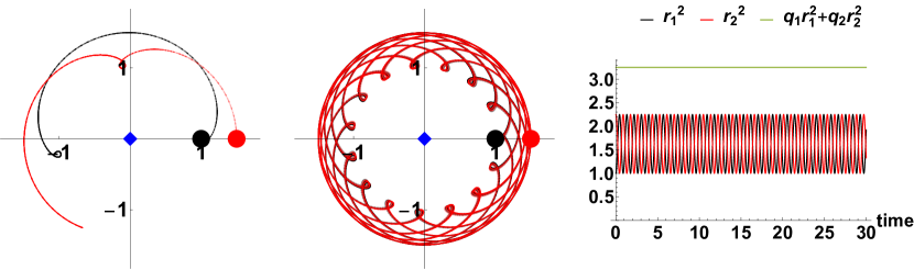
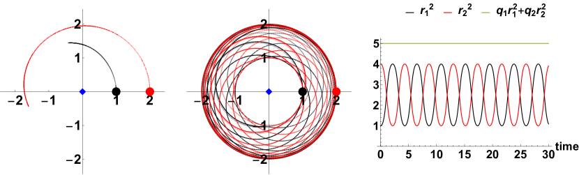
For two vortices with opposite signs (a vortex dipole with ) the quantity remains fixed, allowing each correlated variable to become large. Figure 3 illustrates such behavior for symmetric initial conditions. In contrast, for two vortices with the same sign (), the quantity is fixed, so that the motion of the two vortices remains localized, as seen in Fig. 4 for several symmetric initial conditions.
A few cases are simple to describe. The first is a vortex dipole with and . The four coupled equations now yield the single pair
| (25) |
Since , these equations are equivalent to the condition that is constant. The corresponding dynamics is shown in Fig. 3. Note that this condition ensures the conservation of total energy as seen in Eq. (20).
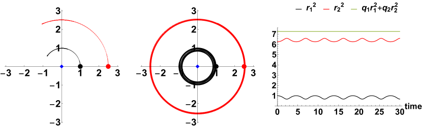
The other example is a pair of equal-charge vortices () with initial conditions along the same radial direction and . Figure 4 shows the resulting dynamics for three cases: , and 2.5. In the first, the interaction of the two vortices dominates the dynamics, whereas for the last, the vortices move essentially independently under the influence of the cone. In each case, we show explicitly that remains fixed.
V Cones with finite boundaries
This section uses the method of images on the bounded sector to determine the appropriate stream function on the bounded cone and the dynamical motion of a vortex with this geometry.
V.1 Finite cone with outer radius
For a finite sector of radius with , the method of images gives the intuitive result (compare Ref. Guen17 )
| (26) |
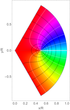
With this complex potential, it is straightforward to visualize the streamlines (black) and lines of constant phase (white) for a positive vortex, as shown in Fig. 5. It is also not difficult to project a similar phase pattern onto the surface of an equivalent three-dimensional truncated cone, as shown in Fig. 6.
The precessional velocity of a positive vortex at on the bounded cone directly follows from Eq. (6):
| (27) |
where the first term is that for an unbounded cone and the second reflects the presence of the outer boundary. For (the planar case), this result reproduces the standard expression from classical hydrodynamics [see, for example, Eq. (B7) in Ref. Guen17 ]. For , the second term vanishes, reproducing the result for an unbounded cone. In contrast, the second term predominates for , when the precessional velocity increases rapidly.
V.2 Truncated unbounded cone with inner radius
A similar formalism describes the motion of a positive vortex on an unbounded truncated cone with where again is the radial coordinate measured along the surface of the cone. The complex potential is now
| (28) |
Here the last term reflects an additional positive quantized vortex at the origin ensuring that the net circulation around the inner boundary vanishes.
Equation (6) readily yields the corresponding precessional velocity
| (29) |
For (the planar case), this result reproduces the classical expression. Here, the second term (reflecting the combined effect of the image and the vortex at the origin) now induces a negative motion when .
V.3 Truncated bounded cone with
As seen in our earlier works on the annulus (Ref. Fett67 ) and on the cylinder (Ref. Guen17 ), the inclusion of two boundaries leads to a doubly infinite set of images. Equation (B3) in Ref. Guen17 gives the complex potential for a vortex in a planar annulus with . The corresponding complex potential for a vortex at in a bounded planar sector with opening angle follows immediately with the conformal transformation :
| (30) |
Here is the complex image of with respect to the outer boundary. Note that lies on the surface of the cone extended beyond the larger boundary.
Equation (6) again yields the translational velocity of the vortex , where
| (31) |
defines the velocity (it is real, despite the explicit appearance of ). The vortex moves uniformly around the bounded cone at fixed . In the limit , this expression properly reduces to that for a planar annulus, given in Eq. (B4) of Ref. Guen17 .
Figure 7 shows for typical values of the cone parameter . When approaches , the outer image dominates and the vortex moves rapidly in the positive direction. In contrast, the behavior for depends on . For not-too-large , the inner image dominates and the vortex simply slows and then reverses, moving in the negative direction as . For larger , however, the translational velocity initially increases with decreasing because of the factor in Eq. (31). Eventually, the inner image dominates and the vortex then moves in the opposite direction.
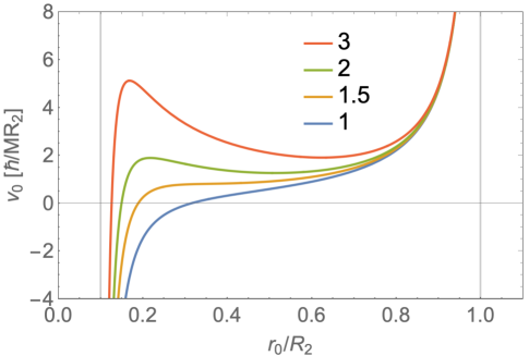
For the special choice (the geometric mean of the inner and outer radii), the identity readily yields the simple result
| (32) |
which is the same as Eq. (8) for an unbounded cone.
VI Outlook and conclusions
Our study of superfluid vortex dynamics on a cone with opening angle starts from a planar sector with opening angle , so that . For a complex variable on the sector, a simple conformal transformation maps this sector onto the full plane.
VI.1 Conjecture for sector with
From this perspective of such a planar sector, it is reasonable to ask what happens when becomes smaller than , remaining real. For definiteness, consider the rational number where and are co-prime numbers and . The sector now has opening angle that exceeds and thus extends beyond the single plane with an overlapping surface. The same conformal mapping now has a Riemann surface with sheets forming a closed cyclic structure. The simplest case is , which leads to a two-fold closed structure for the Riemann surface. An irrational value of leads instead to a Riemann surface which never folds onto itself.
For such an overlapping sector, it appears that the preceding formalism determining Eqs. (8) and (10) for the induced vortex motion on the sector remains valid even for . In particular, a positive vortex should now move in the clockwise direction because is negative.
The more difficult question is what, if any, three-dimensional surface corresponds to a sector of the plane with opening angle and . Evidently this sector overlaps at least part of the plane more than once. The inverse definition requires that become complex with , and real . Correspondingly, is pure imaginary. For this mapping, the definition yields an imaginary value for the three-dimensional vertical coordinate of what was a physical cone for . Hence there may well be no simple three-dimensional real physical surface corresponding to the planar sector with .
VI.2 Comparison with previous work
Vortex dynamics on a plane is an old subject dating back over a century Lamb45 . The plane is flat, so that the question of surface curvature never arises, and such studies are widely applied to quantized vortices in superfluid 4He Donn91 .
Most of the earlier studies of vortices on curved surfaces focused on the total energy and its dependence on the location of the singularities of the relevant fields Vite04 ; Turn10 ; Kami02 ; Ho15 ; Lube92 ; Mach89 . This concentration on the energy yields useful thermodynamic information, but it ignores the very interesting question of the dynamical motion of such superfluid vortices.
The generalization to vortices on curved surfaces has involved two distinct topological situations. Here and in Ref. Guen17 , we considered regions with multiply connected topology and associated winding numbers, specifically a cylinder and a cone. In each case, we studied the associated dynamics of both a single vortex and two vortices (particularly a neutral vortex dipole). The situation on a compact surface such as a sphere differs in that the total vortex charge must vanish Vite04 ; Turn10 ; Lamb45 .
To our knowledge, the only other relevant discussion of vortex dynamics on a curved surface is Secs. 80 and 160 of Ref. Lamb45 , which considers the case of vortices on a sphere. In addition to the restriction to a vortex dipole with zero net charge, Lamb quotes the result for the translational velocity of a vortex dipole on a sphere, based on Kirchhoff’s much earlier electrical studies of a thin spherical conducting layer (see Sec. 80 of Ref. Lamb45 ).
VI.3 Conclusions
We have presented here a description of the dynamics of superfluid vortices on the surface of a cone. We have demonstrated that single vortices precess uniformly around the symmetry axis of the cone (hence conserving self-energy), while configurations with two vortices remain quasiperiodic because of two conserved quantities. As varies between 1 and , the surface of a semi-infinite cone interpolates smoothly between the whole complex plane and an infinite thin cylinder. In the two limits, we have shown explicitly that the results presented here reproduce those well-known behaviors. As a final remark, we note that our previous results on cylindrical surfaces may prove very useful to understand the physics at play in the very recent experiment that studied superfluid 4He adsorbed on carbon nanotubes Mena19 ; Nour19 .
Acknowledgements
The authors thank I. Carusotto, N.-E. Guenther and R. B. Laughlin for insightful discussions. P.M. acknowledges support from Spanish MINECO (FIS2017-84114-C2-1-P) and the “Ramón y Cajal” program. A.L.F. is grateful for the opportunity to visit S. Stringari and the University of Trento in October 2017, where part of this work was done.
Appendix A Vortex motion on a cylinder
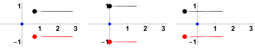
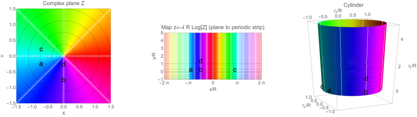
We here review the complex potential for a single vortex on a cylinder. The most straightforward approach Ho15 is to use a conformal map, which links the whole plane (with a coordinate ) to a periodically-repeating strip of width (with a coordinate ):
| (33) |
The action of this map is shown in detail in Fig. 8. In particular, the negative real axis of the complex plane maps to the two infinite sides of the strip, located at coordinates . The strip (shown in the central panel) features periodic boundary conditions, and therefore may be folded onto a three-dimensional cylinder (shown in the right panel). This procedure does not introduce any distortion, so that the transformation is conformal. The coordinates on the cylinder are obtained from the coordinates on the strip by the obvious relations , , and .
The conformal map Eq. (33) may be combined with the complex potential on the plane, Eq. (1), to obtain the corresponding potential on the strip and on the cylinder for a vortex at :
| (34) |
Results for complex potentials, core velocities and interaction energies for finite and infinite cylinders were given in our previous work, Ref. Guen17 . Therein was also a detailed discussion of the close connection of these results with those found earlier in Ref. Fett67 for the topologically equivalent case of vortices on a planar annulus.
References
- (1) V. Vitelli and A. M. Turner Anomalous Coupling Between Topological Defects and Curvature, Phys. Rev. Lett. 93, 215301 (2004).
- (2) A. M. Turner, V. Vitelli, and D. R. Nelson, Vortices on curved surfaces, Rev. Mod. Phys. 82, 1301 (2010).
- (3) N.-E. Guenther, P. Massignan, and A. L. Fetter, Quantized superfluid vortex dynamics on cylindrical surfaces and planar annuli, Phys. Rev. A 96, 063608 (2017).
- (4) N. Schine, A. Ryou, A. Gromov, A. Sommer, and J. Simon, Synthetic Landau levels for photons, Nature 534, 671 (2016).
- (5) K. F. Riley, M. P. Hobson, and S. J. Bence, Mathematical Methods for Physics and Engineering, Cambridge University Press, 3rd ed. (2006).
- (6) R. D. Kamien, The geometry of soft materials: a primer, Rev. Mod. Phys. 74, 953 (2002).
- (7) T.-L. Ho and B. Huang, Spinor Condensates on a Cylindrical Surface in Synthetic Gauge Fields, Phys. Rev. Lett. 115, 155304 (2015).
- (8) A. L. Fetter, Low-lying superfluid states in a rotating annulus, Phys. Rev. 153, 285 (1967).
- (9) H. Lamb, Hydrodynamics, 6th. ed. (Dover Publications, New York, 1945), Chap. VII.
- (10) R. J. Donnelly, Quantized Vortices in Helium II (Cambridge University Press, Cambridge, UK, 1991).
- (11) T. C. Lubensky and J. Prost, Orientational order and vesicle shape, J. Phys. II France 2, 371 (1992).
- (12) J. Machta and R. A. Guyer, Superfluid films on a cylindrical surface, J. Low Temp. Phys. 74, 231 (1989).
- (13) E. Menachekanian, V. Iaia, M. Fan, J. Chen, C. Hu, V. Mittal, G. Liu, R. Reyes, F. Wen, and G. A. Williams, Superfluid onset and compressibility of films adsorbed on carbon nanotubes, Phys. Rev. B 99, 064503 (2019).
- (14) A. Noury, J. Vergara-Cruz, P. Morfin, B. Plaçais, M. C. Gordillo, J. Boronat, S. Balibar, and A. Bachtold, Layering transitions in superfluid helium adsorbed on a carbon nanotube mechanical resonator, arXiv:1901.09642.