Nonparametric Matrix Response Regression with Application to Brain Imaging Data Analysis

Abstract

With the rapid growth of neuroimaging technologies, a great effort has been dedicated recently to investigate the dynamic changes in brain activity. Examples include time course calcium imaging and dynamic brain functional connectivity. In this paper, we propose a novel nonparametric matrix response regression model to characterize the nonlinear association between 2D image outcomes and predictors such as time and patient information. Our estimation procedure can be formulated as a nuclear norm regularization problem, which can capture the underlying low-rank structure of the dynamic 2D images. We present a computationally efficient algorithm, derive the asymptotic theory and show that the method outperforms other existing approaches in simulations. We then apply the proposed method to a calcium imaging study for estimating the change of fluorescent intensities of neurons, and an electroencephalography study for a comparison in the dynamic connectivity covariance matrices between alcoholic and control individuals. For both studies, the method leads to a substantial improvement in prediction error.

1 Introduction

1.1 Motivation

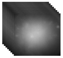
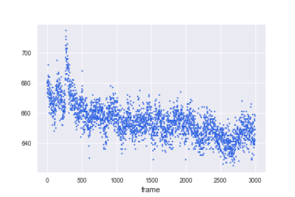
Figure 2: (a) A sequence of frames (b) scatterplot for a fixed voxel of coordinate (200,60) over frames. This figure appears in color in the electronic version of this article, and any mention of color refers to that version.

Neuroimaging techniques have been widely used in both scientific research and clinical applications, e.g., calcium imaging, electroencephalography (EEG), magnetic resonance imaging and functional magnetic resonance imaging. Those techniques provide a great opportunity for (1) the investigation of neuron activities at the cellular level, e.g., the quantitative estimation of the intracellular calcium signals; and (2) a better understanding of the dynamic changes in brain activity as well as their associations with disease and other clinical information. Here we briefly discuss two relevant examples. More details about these examples will be given in Section 2. The first example is related to the fluorescent calcium imaging, which is an emerging popular technique for observing the spiking activity of large neuronal populations over the past decade. This new technology allows scientists to observe the locations of neurons and the times at which they fire using two-photon microscopy (Helmchen and Denk, 2005; Petersen et al., 2018), resulting in a data set as a video clip, i.e., a sequence of 2D images taken over the time. The scientific questions of interest are to identify the major neurons and model their spiking activity over the time; and calcium imaging techniques provide a unique opportunity to address those questions because of its ability to directly collect the rich and accurate measurements at the cellular level. As shown in Figure 2(a), the images are quite noisy and structured-sparse (in the sense that the signal level is low at the boundary for most images), yet contains rich information (the video clip we study in this paper composes 3,000 picture frames with several obvious major neurons located in the center of the image firing for multiple times). Thus it is important and non-trivial to develop an automatic-yet-flexible pipeline for analyzing such type of data sets.

Our second example is the brain functional connectivity analysis. Functional connectivity refers to the coherence of the activities among distinct brain regions (Horwitz, 2003), and it provides novel insights on how distributed brain regions are functional integrated (Biswal et al., 1995, 2010; Fox et al., 2005). In general, studies of functional connectivity are based on the temporal correlation between spatially remote neurophysiological events (Friston, 1994) with an implicit assumption that the functional connectivity is at the same level during the observation period. Recently, functional connectivity has been shown to fluctuate over time (Chang, Liu, Chen, Liu, and Duyn, 2013), implying that measures assuming stationarity over a full scan may be too simplistic to capture the full brain activity. Since the initial findings, researchers have investigated the so-called dynamic functional connectivity; see (Calhoun et al., 2014; Calhoun and Adali, 2016; Preti et al., 2017; Zhang et al., 2016) for reviews to date. It then makes sense to represent the connectivity as a covariance matrix and model its change over the time and other clinical factors of interest. As shown in Figure 4, we analyze an EEG data set to study the dynamic functional connectivity between alcoholic and non-alcoholic individuals. There is a significant difference in terms of image pattern and temporal correlation between two groups of participants.

1.2 Challenges and contributions

Statistically speaking, it is natural to quantify the association between 2D image outcomes and the predictors such as time, patient demographics, and other disease predictors by a regression model. Such regression model will also serve as a useful tool for smoothing and denoising purposes. However, several challenges remain unaddressed in the literature. First, the neuroimaging data obtained from the experiments, even after some pre-processing steps, are often noisy and taking complex structure, such as spatial/temporal correlation, low rankness, and sparsity. Such structural information provides useful scientific and clinical insight, but also imposes additional challenges to statistical analysis and computation.

Secondly, existing regression approaches are mainly focused on linear models and image predictors in the literature, where the linearity assumption, as much as it simplifies the computational/theoretical investigation, does not quite meet the need to accurately model the nonlinear pattern between predictors and the image outcomes. For example, we performed a preliminary analysis on the calcium imaging data collected by Ilana Witten’s lab at the Princeton Neuroscience Institute (Petersen et al., 2018). Figure 2(b) shows a scatter plot of the changes of fluorescent intensities across time from a randomly selected pixel of the 2D-image. The scatter plot shows a clear nonlinear pattern, which will be neglected by linear models. Note that classical nonlinear regression approaches such as Nadaraya-Watson method can not be directly used in our case to model the matrix-valued image responses, since doing so is equivalent to vectorizing the 2D-image data, which destroys the underlying spatial information of the image.

In this paper, we propose a novel low rank nonparametric regression approach to take account of the matrix structure of the image data by solving a nuclear norm regularization problem. By the singular value thresholding algorithm (Cai et al., 2010), we show that our estimator has a closed-form solution for each fixed bandwidth and regularization parameter. To efficiently select these tuning parameters, we derive a Bayesian information criterion (BIC) based on our model and estimation procedure. For theoretical justification, we derive the risk bound for our nonparametric estimator. We show that the rank of the true function can be consistently estimated as well.

Here we highlight our contributions in this paper. First, we propose a novel nonparametric matrix response regression model that is capable of modeling the nonlinear relationship between image responses and predictors. There are some related works on (generalized) linear models for matrix-valued data. For example, Zhou and Li (2014) proposed a class of regularized matrix linear regression model by treating matrix data as covariates; Hu et al. (2020) proposed a linear discriminant analysis approach for the classification of high-dimensional matrix-valued data; Wang and Zhu (2017) developed a generalized scalar-on-image regression model via total variation; Ding and Cook (2018) studied the matrix response linear regression model using envelope methods; Kong et al. (2020) proposed a low-rank linear regression model with high-dimensional matrix response and high dimensional scalar covariates. Li and Zhang (2017); Zhang and Li (2017) studied the tensor linear regression problem with a multidimensional array response and a vector predictor. To the best of our knowledge, no work has been done on using nonparametric models for matrix data analysis. Second, our nonparametric estimator is easy to derive and has a closed-form solution, which makes it computationally more efficient than the state-of-art multivariate varying coefficient model (Zhu et al., 2011; Zhu et al., 2012). The tuning process is also simple thanks to the derived analytic form of BIC, which is not straightforward for the proposed nonparametric matrix response model. Thirdly, we develop the asymptotic theories including the risk bound and rank consistency for the method, which directly connects to the existing work on nonparametric statistics theory, hence rendering for a deeper understanding of such type of models. Finally, as demonstrated in both real data analysis examples, the proposed nonparametric model is simple, ready-to-use, manages to fit the nonlinear changes in brain signals very well and has a substantial improvement in the prediction error. The low-rankness assumption seems amenable in practice. We are currently developing a computational package for the proposed methodology and we expect it to have a major impact in the neuroimaging community.

2 Data applications

In this section we provide more details about the two motivating data examples and highlight their scientific merit and associated statistical challenges.

2.1 Fluorescent calcium imaging

Calcium ions generate versatile intracellular signals that control key functions in all types of neurons, including the control of heart muscle cell contraction and the regulation of vital aspects of the entire cell cycle. Fluorescent calcium imaging is a sensitive method for monitoring neuronal activity (Mao et al., 2001). It makes use of the fact that in living cells, most depolarizing electrical signals are associated with calcium ions influx attributable to the activation of one or more of the numerous types of voltage-gated calcium ions channels, abundantly expressed in the nervous system (Tsien and Tsien, 1990; Stosiek et al., 2003). Imaging calcium in neurons is particularly important because calcium signals exert their highly specific functions in well-defined cellular subcompartments (Grienberger and Konnerth, 2012). The advantage of calcium imaging is that it allows real-time analyses of individual cells and even subcellular compartments. At the same time it readily permits simultaneous recordings from many individual cells (Stosiek et al., 2003).

When a neuron fires, voltage-gated calcium channels in the axon terminal open and then calcium floods the cell. Such changes in concentration of calcium ions are detected by observing the fluorescence of calcium indicator molecules. Therefore, not surprisingly, intracellular calcium concentration becomes an important surrogate marker for the spiking activity of neurons in the absence of effective voltage imaging approach and is commonly used when analyzing local neuronal circuits in vivo and in vitro (Petersen et al., 2018; Grienberger and Konnerth, 2012). However, the available experimental techniques still lead to noisy and spatial-temporally-subsampled observations of true underlying signals (Pnevmatikakis et al., 2012). The calcium trace is smeared which restricts the extraction of quantities of interest such as spike trains of individual neurons (Rahmati et al., 2016). The spatio-temporal smoothing of the calcium profile remains a difficult problem due to the high dimensionality and complex structure of calcium imaging data. New methods that are capable of characterizing the dynamic changes of calcium imaging videos and performing the spatio-temporal smoothing of the calcium data are largely needed.

2.2 Dynamic functional connectivity

Functional connectivity measures statistical dependence between the time series signals obtained from different brain regions. The functional connectivity has been investigated in a wealth of literature with various analysis tools, and has applications in different imaging modalities such as functional magnetic resonance imaging (fMRI), Electroencephalography (EEG), Magnetoencephalography (MEG) and Positron emission tomography (PET). The functional connectivity is built upon the assumption that the connectivity is stationary in nature.

More recently, the dynamic behavior of functional connectivity was revealed, suggesting that connectivity between different brain regions exhibits meaningful variation over time. Hence it provides a more detailed representation of brain function than the traditional static functional connectivity analysis. Several previous studies have suggested that the dynamic functional connectivity can be used to characterize different psychiatric and neurodegenerative disorders such as schizophrenia (Damaraju et al., 2014), Parkinson’s disease (Engels et al., 2018; Zhu et al., 2019) and Alzheimer’s disease (Niu et al., 2019). One of the most common ways to quantify the dynamic functional connectivity is by estimating the dynamic covariance matrices using a slide window approach. The dynamic covariance matrices have proven to be very useful in revealing the change patterns of brain network over the time. In addition, studying the association between those matrices with clinical factors and disease outcomes may provide useful insights for future clinical practice such as disease prediction. Due to the high level of noises in the original imaging data, accurate estimation and denoising procedures are largely needed. By pooling the estimates of the covariance matrices obtained from different sliding windows together and taking the structure of matrices into account, our newly proposed model can help improve the estimation accuracy of these dynamic covariance matrices.

3 Method

3.1 Model

Suppose we observe a set of 2D-images and some scalar predictors from $n$ study subjects. Let $Y_{i}$ be a $p\times q$ matrix representing the 2D-image from the $i$th subject, and $X_{i}=(x_{i1},\ldots,x_{is})^{T}$ be an $s\times 1$ vector denoting the scalar covariates of interest (e.g., time and disease predictors). We propose the following nonparametric matrix response model,

$$E(Y_{i}|X_{i})=g(X_{i}),$$ (1)

where $g(\cdot):\mathbb{R}^{s}\rightarrow\mathbb{R}^{p\times q}$ is a nonparametric matrix-valued function that quantifies the nonlinear relationship between (each pixel of) $Y_{i}$ and $X_{i}$. Since $g(x)$ is a $p\times q$ matrix, we will also impose a structure constraint on $g$ for scientific interpretability and regularization purpose.

Our goal is to estimate the nonparametric function $g$. A commonly used estimator is the Nadaraya-Watson estimator for matrix data, which can be written as

$$\widehat{g}_{\text{nw}}(x)=\frac{\sum_{i=1}^{n}K_{H}(x-X_{i})Y_{i}}{\sum_{i=1}^{n}K_{H}(x-X_{i})},$$ (2)

where $K_{H}(\cdot)=\frac{1}{|H|}K(H^{-1}\cdot)$, $K(\cdot)$ is a kernel density function, and $H=\text{diag}(h_{1},h_{2},\cdots,h_{s})$ is a bandwidth matrix. It is often assumed that $h_{1}=\cdots=h_{s}=h$ for computational convenience.

However, the Nadaraya-Watson estimator is a “naive” estimator in our case because it does not utilize the underlying structure of the matrix response $Y_{i}$. In particular, the estimator in (2) can also be obtained by vectorizing $Y_{i}$, applying the Nadaraya-Watson estimator for the vectorized data, and transforming the estimator back to a matrix. To account for the matrix structure, we take another look at the estimator in (2), which can be obtained by solving the following optimization,

$$\widehat{g}_{\text{nw}}(x)={\rm argmin}_{Y}\sum_{i=1}^{n}K_{H}(x-X_{i})\|Y_{i}-Y\|^{2}_{F},$$ (3)

where $\|\cdot\|_{F}$ is the Frobenius norm of a matrix.

To further exploit the underlying structure of the 2D response, we introduce a penalty on $Y$ and propose to solve

$$\widehat{g}(x)={\rm argmin}_{Y}\left\{\frac{1}{2n}\sum_{i=1}^{n}K_{H}(x-X_{i})\|Y_{i}-Y\|^{2}_{F}+\lambda_{n}\|Y\|\right\},$$ (4)

where $\lambda_{n}$ is the tuning parameter and $\|\cdot\|$ is some norm of a matrix. Possible choices are nuclear norms, total variation norms, and their combination; and each of those norms will have different regularization effects on the image outcomes. For this paper, we mainly focus on the nuclear norm regularization for illustration, i.e., writing $\|Y\|$ as $\|Y\|_{*}$, which is defined as the sum of all singular values of the matrix $Y$. The nuclear norm is very popular in 2D-image denoising (Gu et al., 2014; Gao et al., 2020). The underlying true 2D-image is often of low rank or approximately low rank, and the nuclear norm regularization can help recover the low rank structure given a noisy image (Chen et al., 2013). In our case, $\widehat{g}(x)$ can be regarded as an image estimate at the point $x$, and therefore the penalty $\|Y\|_{*}$ can push for a low rank representation of the image estimate.

In Section 6 of Supporting Information, we show that solving (4) is equivalent to solving

$$\begin{split}\widehat{g}(x)={\rm argmin}_{Y}\left\{\frac{1}{2}\|\widehat{g}_{\text{nw}}(x)-Y\|^{2}_{F}+\frac{n\lambda_{n}}{\sum_{i=1}^{n}K_{H}(x-X_{i})}\|Y\|_{*}\right\}.\end{split}$$ (5)

The optimization problem (5) can be solved using the following proposition restated from Cai et al. (2010).

Proposition

Consider the singular value decomposition of a matrix $Y\in R^{p\times q}$ with rank $r$,

$$Y=U\Sigma V^{\ast},\text{\quad}\Sigma=\text{diag}(\{\sigma_{j}\}_{1\leq j\leq r}),$$

where $U$ and $V$ are $p\times r$ and $q\times r$ matrices respectively with orthonormal columns, and singular values $\{\sigma_{j}\}_{1\leq j\leq r}$ are positive (we only consider these $r$ non-zero singular values given that the rank of $Y$ is $r$). The soft-thresholding operator $D_{\tau}$ is defined as

$$D_{\tau}(Y)=UD_{\tau}(\Sigma)V^{\ast},D_{\tau}(\Sigma)=\text{diag}[\{(\sigma_{j}-\tau)_{+}\}_{1\leq j\leq r}],$$ (6)

where $(\cdot)_{+}$ is the positive part of $(\cdot)$. Then $D_{\tau}(Y)$ satisfies

$$D_{\tau}(Y)=\arg\min_{X}\left\{\frac{1}{2}\|Y-X\|_{F}^{2}+\tau\|X\|_{\ast}\right\},$$

where $\|X\|_{\ast}$ is defined as the nuclear norm of the matrix $X$.

By Proposition 3.1, our estimator in (4) can be obtained using the following algorithm. The proof is given in Section 7 of Supporting Information.

Algorithm 1 Algorithm to solve the optimization problem (4).

Input: $\{(X_{i},Y_{i}),1\leq i\leq n\},x,H,\lambda_{n}$.
Step 1: Perform singular value decomposition of $\widehat{g}_{\text{nw}}(x)=\frac{\sum_{i=1}^{n}K_{H}(x-X_{i})Y_{i}}{\sum_{i=1}^{n}K_{H}(x-X_{i})}$, and denote it by $U\Sigma V^{\ast}$. The diagonal matrix $\Sigma=\text{diag}(\{\sigma_{j}\}_{1\leq j\leq r})$, where $\sigma_{1}\geq\sigma_{2}\geq\ldots\geq\sigma_{r}>0$ with $r$ being the rank of $\Sigma$.
Step 2: Set $\tau=\frac{n\lambda_{n}}{\sum_{i=1}^{n}K_{H}(x-X_{i})}$, and calculate the soft-thresholding operator $D_{\tau}(\Sigma)=\text{diag}(\{(\sigma_{j}-\tau)_{+}\}_{1\leq j\leq r})$.
Step 3: Calculate $\widehat{g}(x)=UD_{\tau}(\Sigma)V^{\ast}$.
Output: $\widehat{g}(x)$.

3.2 Bayesian information criterion

The optimization problem (4) involves two tuning parameters, the bandwidth $h$ and the regularization parameter $\lambda$. The choices of these two parameters are critical as they control the temporal smoothing level and the spatial low-rank level, respectively. In this paper, we derive a Bayesian information criterion (BIC) to select them. Define $\widetilde{\lambda}=\frac{n\lambda_{n}}{\sum_{i=1}^{n}K_{H}(x-X_{i})}$ and $\widehat{Y}_{i}(\widetilde{\lambda})=\widehat{g}(X_{i})$. Without loss of generality, we assume $p\geq q$ and denote the singular values of $\widehat{Y}_{i}(\widetilde{\lambda})$ by $b_{i1}(\widetilde{\lambda})\geq\cdots\geq b_{iq}(\widetilde{\lambda})\geq 0$. From Algorithm 1, it can be seen that the singular values of $\widehat{Y}_{i}(\widetilde{\lambda})$ are corresponding truncated singular values of $\widehat{g}_{\text{nw}}(X_{i})$. Since we are considering a least squared error loss in (4), the BIC can be defined as

$$\textsc{bic}(\widetilde{\lambda})=npq\log\left\{\frac{1}{npq}\sum_{i=1}^{n}\|Y_{i}-{\widehat{Y}}_{i}(\widetilde{\lambda})\|_{F}^{2}\right\}+\log(npq)\text{df}(\widetilde{\lambda}),$$ (7)

where $\text{df}(\widetilde{\lambda})$ can be estimated based on the result in the following proposition. The proof of the proposition is deferred to the Supporting Information.

Proposition

Denote $\widehat{g}_{\text{nw}}(X_{i})$’s singular values by $\sigma_{i1}\geq\sigma_{i2}\geq\cdots\geq\sigma_{ir_{i}}>0$ and $\sigma_{ik}=0$ for $k>r_{i}$. An unbiased estimator of the degree of freedom $df(\widetilde{\lambda})$ is

$$\widehat{df}(\widetilde{\lambda})=K_{H}(0)\sum_{i=1}^{n}\frac{\widehat{df}_{i}(\widetilde{\lambda})}{\sum_{j=1}^{n}K_{H}(X_{i}-X_{j})},\text{\quad where}$$

$$\widehat{df}_{i}(\widetilde{\lambda})=\sum_{k=1}^{q}{1}_{\{b_{ik}(\widetilde{\lambda})>0\}}\Big{\{}1+\sum_{1\leq j\leq p,j\neq k,k\leq r_{i}}\frac{\sigma_{ik}(\sigma_{ik}-\widetilde{\lambda})}{\sigma_{ik}^{2}-\sigma_{ij}^{2}}+\sum_{1\leq j\leq q,j\neq k,k\leq r_{i}}\frac{\sigma_{ik}(\sigma_{ik}-\widetilde{\lambda})}{\sigma_{ik}^{2}-\sigma_{ij}^{2}}\Big{\}}.$$ (8)

4 Theory

In this section, we present theoretical results of the estimation procedure in (4), including a risk bound of the regularized estimator and a rank consistency result. Denote the strength of regularization as $\lambda_{n}$ and the true response as $g(X)$ given covariates $X$. Assume $g(X)$ has unknown rank $r$ and denote the global minimizer of (4) by $\widehat{g}(X)$. For any two sequences of real numbers $a_{n}$ and $b_{n}$, we write $a_{n}\asymp b_{n}$ if there exist universal positive constants $C_{1}$ and $C_{2}$ such that $C_{1}b_{n}\leq a_{n}\leq C_{2}b_{n}$. We define $a\vee b=\max(a,b)$ and $a\wedge b=\min(a,b)$ for any $a,b\in\mathbb{R}$. With a little abuse of the notation, we use $C$ to denote a universal constant whose value may change in different context but does not affect the results. For a matrix $A$ and a sequence of real numbers $a_{n}$, we write $A=O_{p}(a_{n})$ or $A=o_{p}(a_{n})$ if every element of $A$ is $O_{p}(a_{n})$ or $o_{p}(a_{n})$.

Let $g_{jk}(x)$ be the $(j,k)$-th component of $g(x)$. We make the following assumptions: We assume that $|g_{jk}(x)-g_{jk}({y})|<C\|{x-y}\|^{\alpha_{2}}$ with $\alpha_{2}>0$, $1\leq j\leq p,1\leq k\leq q$ for any $\|{x-y}\|<\delta$ and some $C>0$, when $\delta>0$ is sufficiently small. We also assume that the pixels in the residual matrix, $E_{i}=Y_{i}-g(x_{i})$, are independent and identically distributed (i.i.d) for every $i=1,\ldots,n$. Assume that $npqh^{2\alpha_{2}+s}\rightarrow\infty$, $nh^{2s}\rightarrow\infty$, and $pqh^{2\alpha_{2}}\rightarrow 0$ as $n\rightarrow\infty$. We assume that the kernel function $K(\cdot)$ is bounded on $\mathbb{R}^{s}$. In other words, there exists a universal constant $k_{\text{max}}>0$ (i.e, $k_{\max}$ does not depend on $x$) such that $K(x)\leq k_{\max}$ and $K_{H}(x)\leq h^{-s}k_{\text{max}}$ for every $x\in\mathbb{R}^{s}.$ Moreover, we assume there exist universal constants $C_{f},c_{f}>0$ such that the density function of covariate $x$ satisfies $c_{f}\leq f(x)\leq C_{f}$ for every $x$.

Assume that $n^{-1/2}(p\wedge q)\to 0$, $(pq)^{1/2}h^{\alpha_{2}}(p\wedge q)^{1/2}\lambda_{n}^{-1}\to 0$, $\lambda_{n}(p\wedge q)^{2}\to 0$, and $\frac{pq(p\wedge q)}{n\lambda_{n}^{2}}\to 0$ as $n\rightarrow\infty$.

Assumption 4 assumes the $\alpha_{2}$-smoothness for each element of the nonparametric function $g(x)$. This assumption is commonly used in multivariate function estimation literature such as Scott (2015). It is possible to extend the results for anisotropic case in the future work based on the techniques developed in this paper. The i.i.d assumption for the pixels in the residual is needed for showing consistency result, and we have conducted a sensitivity analysis in the simulation to show that our proposed method is robust to the violation of this assumption. Assumption 4 is required for estimation consistency as it imposes constraints on the matrix size and the bandwidth. Assumption 4 is satisfied for most kernel density functions. The boundedness condition for the density function of $x$ will hold if $x$ is defined on a compact support and the density is continuous. Assumption 4 is needed for rank consistency. With these assumptions, we can state the two main theorems of this paper. Their proofs are given in the Supporting Information.

Theorem 4.1

Suppose that Assumptions 4–4 hold. We consider two cases for $p$ and $q$ (e.g., whether they diverge or not).

(1) If both $p$ and $q$ are fixed, let $h\asymp(\frac{\log n}{n})^{\frac{1}{2\alpha_{2}+s}\wedge\frac{1}{2s}}$ and $\lambda_{n}\asymp h^{\alpha_{2}}$, then with probability tending to 1,

$$\|\widehat{g}(x)-g(x)\|_{F}^{2}\leq Cr\left(\frac{\log n}{n}\right)^{\frac{2\alpha_{2}}{2\alpha_{2}+s}\wedge\frac{\alpha_{2}}{s}}.$$

(2) If $p\vee q\rightarrow\infty$ and $p\vee q=o\left(n^{\frac{\alpha_{2}}{2\alpha_{2}+s}}\wedge(\frac{n}{\log n})^{\frac{\alpha_{2}}{2s}}\right)$, then by letting $h\asymp n^{-\frac{1}{2\alpha_{2}+s}}\vee(\frac{\log n}{n})^{\frac{1}{2s}}$ and $\lambda_{n}=h^{\alpha_{2}}(pq)^{1/2}$, with with probability tending to 1, we have

$$\|\widehat{g}(x)-g(x)\|_{F}^{2}\leq Cpqr\left\{n^{-\frac{2\alpha_{2}}{2\alpha_{2}+s}}\vee(\frac{\log n}{n})^{\frac{\alpha_{2}}{s}}\right\}.$$

Note that the risk bound involves two quantities $n^{-\frac{2\alpha_{2}}{2\alpha_{2}+s}}$ and $(\frac{\log n}{n})^{-\frac{\alpha_{2}}{s}}$. As the number of predictors $s$ increases, it becomes more difficult to estimate $g(x)$. Meanwhile, $h^{s}$ is involved when proving strongly restricted convexity of the loss function. A larger value of $s$ indicates smaller probability of the loss function being strong restricted convex. In contrast, $\alpha_{2}$ describes the smoothness of $g(x)$. A larger $\alpha_{2}$ leads to a smaller risk bound and a faster convergence rate. The rate here holds uniformly for any $x$ satisfying Assumption 3; and the true rank of matrix $r$ does not have to be finite for case (2).

If $p$ and $q$ are fixed and $s\leq 2\alpha_{2}$, the optimal bandwidth $h$ can be chosen arbitrarily close to $n^{-\frac{1}{2\alpha_{2}+s}}$, which leads to the same convergence rate (with additional logarithmic factor) for estimating an $\alpha_{2}$-smooth, $s$-dimensional function without regularization. When $\max(p,q)\rightarrow\infty$, if we further assume $s\leq\alpha_{2}$ and choose $nh^{2\alpha_{2}+s}\asymp\frac{(\sqrt{p}+\sqrt{q})^{2}}{pq}$ and $\lambda_{n}\asymp(pq)^{1/2}\left\{\frac{(\sqrt{p}+\sqrt{q})^{2}}{npq}\right\}^{\frac{\alpha_{2}}{2\alpha_{2}+s}}$, as we let $\lambda_{n}\rightarrow 0$ and $nh^{2s}\rightarrow 0$, we obtain $\max(p,q)=o(n^{\frac{\alpha_{2}}{\alpha_{2}+s}})$. This is the necessary condition for $\widehat{g}(x)$ being consistent. The assumption $s\leq\alpha_{2}$ rules out the case where there are too many covariates in the model.

Next we present the rank consistency result. We consider three general cases for different values of $p$ and $q$ (e.g., whether they diverge or not) and discuss the corresponding choices of $\lambda_{n}$ and $h$ as follows,

• If both $p,q$ are fixed, we can choose $h\asymp(\frac{\log n}{n})^{\frac{1}{2\alpha_{2}+s}\wedge\frac{1}{2s}}$ and $\lambda_{n}\asymp h^{\alpha_{2}}\log n$.

• If $p\wedge q$ is finite, and $p\vee q\to\infty$ satisfying $(\log n)^{2}(p\vee q)=o\left\{(\frac{n}{\log n})^{\frac{\alpha_{2}}{s}}\wedge n^{\frac{2\alpha_{2}}{2\alpha_{2}+s}}\right\}$, then we choose $h=(\frac{\log n}{n})^{\frac{1}{2s}}\vee n^{-\frac{1}{2\alpha_{2}+s}}$ and $\lambda_{n}\asymp(p\vee q)^{1/2}h^{\alpha_{2}}\log n$.

• If $p\asymp q$, and $p\to\infty$, then we let $h\asymp(\frac{\log n}{n})^{\frac{1}{2s}}\vee n^{-\frac{1}{2\alpha_{2}+s}}$ and $\lambda_{n}\asymp p^{\frac{3}{2}}h^{\alpha_{2}}(\log n)$. In addition, we assume $(\log n)^{\frac{2}{7}}p=o(h^{-\frac{2\alpha_{2}}{7}})$.

Theorem 4.2

Suppose that Assumptions 4–4 hold, and one of the cases in (C1)–(C3) holds, then $\widehat{g}(x)$ is consistent and rank consistent, i.e.,

$$P\left[\text{rank}\{\widehat{g}(x)\}=\text{rank}\{g(x)\}\right]\to 1,\text{\quad as }n\to\infty.$$

It can be seen that rank consistency requires stronger assumptions on $p,q$ compared with those in Theorem 4.1. For instance, the desired $\lambda_{n}$ is much larger than the one from the previous theorem. Meanwhile, $pq$ is not allowed to be greater than $n$ for rank consistency. Assumption 4 is an extra condition needed for rank consistency but not for estimation consistency. The rank consistency result holds uniformly for any $x$ satisfying Assumption 4.

5 Simulation

In this section, we evaluate the empirical performance of our method and other competing methods. We consider both univariate and multivariate $X$, different nonparametric functions and different correlation structures of the random error $E_{i}$, where $E_{i}=Y_{i}-g(x_{i})$.

5.1 Univariate predictor

Setting I: We set the dimensions of the image $p=q=64$, and set the $(j,k)$-th element of the nonparametric function $g(x)_{jk}=\{\sin(10\pi x)+\cos(10\pi x)+0.1(j+k)\}*B_{jk}$, $1\leq j,k\leq 64$, where $0\leq x\leq 1$ and $B_{jk}$ is the $(j,k)$-th element of the true signal $B$. The true signal $B$ is generated from a 64-by-64 image, where we consider three shapes: a cross, a square and a T-shape. We have plotted the true shapes in Figure 1(a)(b)(c), where we assign $B$ a value of 5 for black regions and 0 for white regions. The sample size is set at $n=200,500$. The covariates $\{x_{i}\},i=1,2,\dots,n$ are equally spaced on [0,1]. The response $Y_{i}$ is generated from $Y_{i}=g(x_{i})+E_{i},$ where $\text{vec}(E_{i})$’s are i.i.d $N(0,I_{pq})$. The optimal bandwidth $h$ and $\lambda$ are selected by BIC. For the kernel function, we use the standard gaussian kernel density defined as $K(x)=\exp(-x^{2}/2)/\sqrt{2\pi}$. We compare our method with the naive Nadaraya-Watson estimator and the Lasso estimator, where the Lasso estimator is obtained by solving the following optimization problem

$$\widehat{g}_{\text{lasso}}(x)={\rm argmin}_{Y}\left\{\frac{1}{2n}\sum_{i=1}^{n}K_{H}(x-X_{i})\|Y_{i}-Y\|^{2}_{F}+\lambda_{n}\|Y\|_{1}\right\},$$ (9)

where $\|Y\|_{1}$ is defined as the sum of the absolute values of all the elements of the matrix $Y$. We also use the BIC as defined in (7) to choose the tuning parameter for Lasso. Here the degree of freedom can be obtained by the chain rule as

$$\widehat{\text{df}} =\sum_{i=1}^{n}\text{tr}\left(\frac{\partial\text{vec}(\widehat{Y}_{i})}{\partial\text{vec}(Y_{i})}\right)=\sum_{i=1}^{n}\sum_{j=1}^{p}\sum_{k=1}^{q}\frac{\partial\widehat{Y}_{ijk}}{\partial\widehat{g}_{ijk(nw)}}\frac{\partial\widehat{g}_{ijk(nw)}}{\partial Y_{ijk}}$$

$$=\sum_{i=1}^{n}\frac{K_{H}(0)}{\sum_{j=1}^{n}K_{H}(X_{i}-X_{j})}\|\text{sign}(\text{vec}(\widehat{Y}_{i}))\|_{1},$$

where we have used the fact that $\frac{\partial\widehat{Y}_{ijk}}{\partial\widehat{g}_{ijk(nw)}}=|\text{sign}(\widehat{Y}_{ijk})|$.

In each replication, we generate $n$ samples as the training set and another 500 samples as the test set. We report the integrated error $\int_{x}\|\widehat{Y}(x)-Y(x)\|_{F}^{2}dx$, which can be approximated by $\frac{1}{500}\sum_{i=1}^{500}\|\widehat{Y}(x_{i}^{test})-Y(x_{i}^{test})\|_{F}^{2}$. Table 1 shows the average integrated test error by our method, naive Nadaraya-Watson estimator and Lasso estimator based on 100 Monte Carlo replicates. We also report the average selected rank by our method using BIC, defined as $\frac{1}{n}\sum_{i=1}^{n}\text{rank}\{\widehat{Y}(x_{i})\}$.

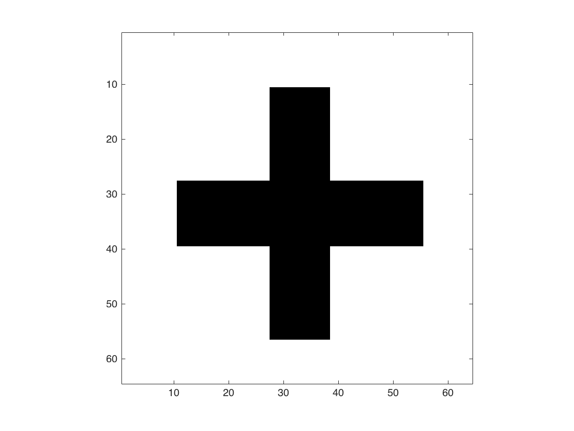
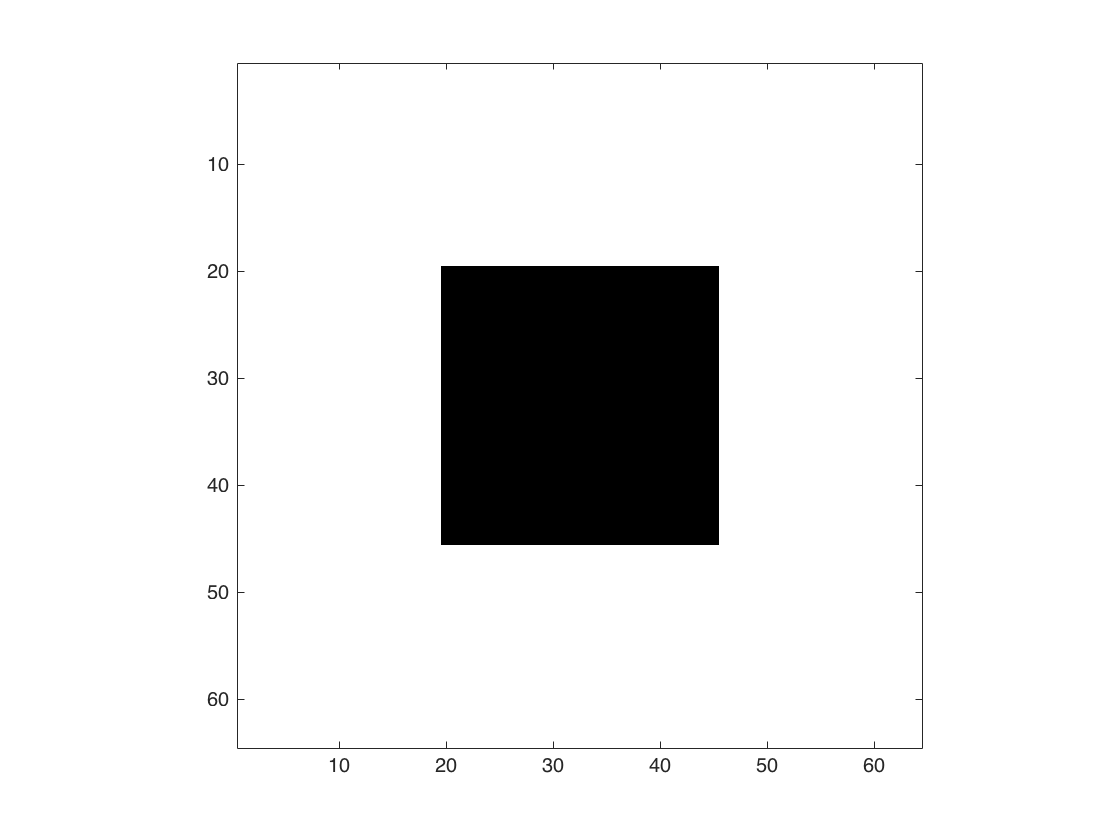
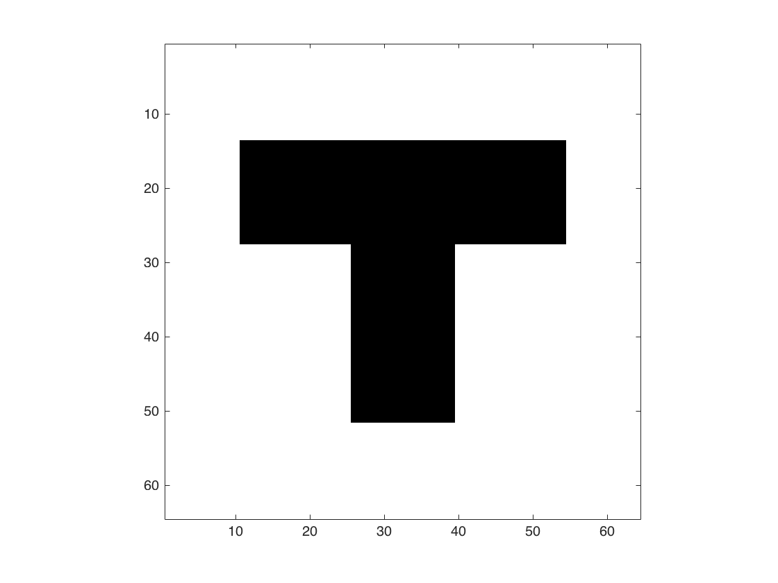
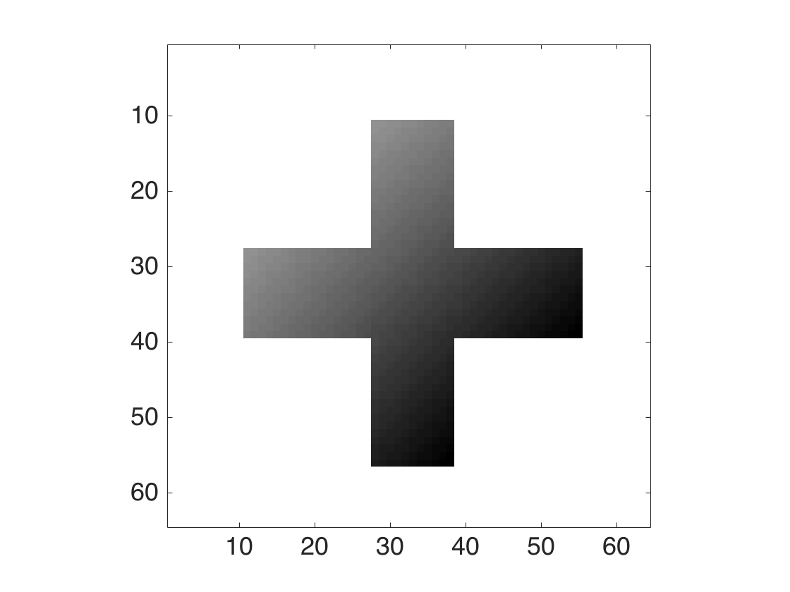
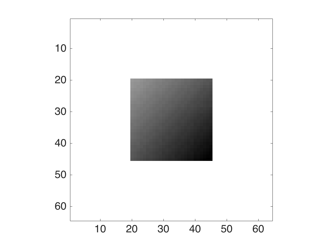
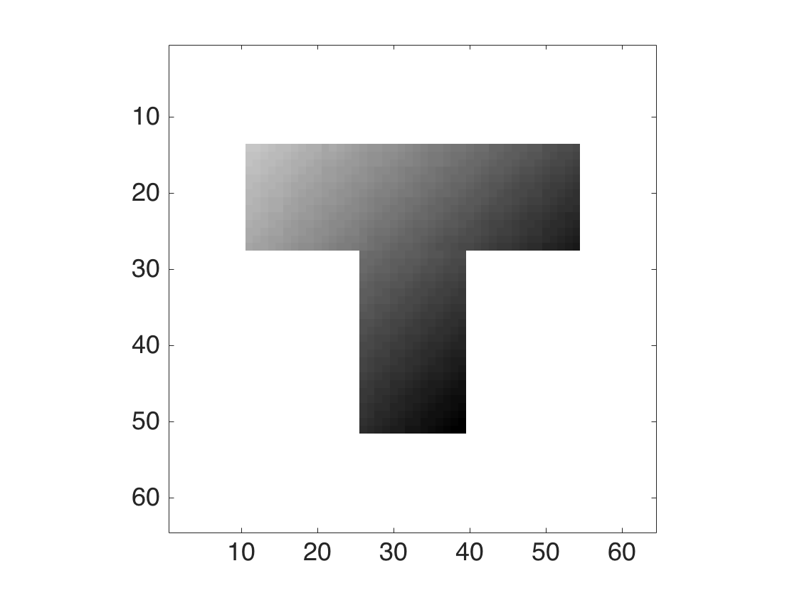
Figure 1: (a)-(c): true signals, (d)-(f): recovered signals

From the results, we can see that our method performs better than Nadaraya-Watson estimator and Lasso estimator in all cases. In addition, our method can estimate the true rank of the image accurately. We have plotted the recovered signals from one randomly selected Monte Carlo study in Figure 1(d)(e)(f), and our method manages to recover the true signals very well.

Table 1: Simulation results: mean of integrated test error and associated standard errors obtained from our method, NW estimator, and Lasso, the average selected rank and true rank are reported for three different shapes $B$. The results are based on 100 Monte Carlo replications.

Setting I	$n$	Shape	Our method	NW	Lasso	Selected rank	True rank
		Cross	4458 (0.70)	6024 (0.96)	5148 (0.81)	3.53 (0.004)	4
	200	Square	4288 (0.82)	6107 (0.99)	4875 (0.83)	2.00 (0.000)	2
		Tshape	4472 (0.76)	6094 (0.98)	5193 (0.92)	3.22 (0.006)	4
		Cross	4306 (0.41)	5009 (0.52)	4560 (0.48)	3.99 (0.000)	4
	500	Square	4186 (0.41)	4803 (0.48)	4440 (0.45)	2.01 (0.000)	2
		Tshape	4255 (0.60)	5042 (0.51)	4579 (0.49)	3.52 (0.007)	4
Setting II	$n$	Shape	Our method	NW	Lasso	Selected rank	True rank
		Cross	4656 (2.23)	6120 (3.47)	5528 (3.49)	6.64 (0.009)	4
	200	Square	4463 (2.31)	5785 (3.27)	5169 (4.72)	4.42 (0.009)	2
		Tshape	4667 (2.49)	6017 (3.65)	5591 (3.74)	6.52 (0.008)	4
		Cross	4403 (1.23)	5240 (1.96)	4769 (1.71)	6.90 (0.008)	4
	500	Square	4296 (1.10)	5036 (1.64)	4692 (1.68)	4.76 (0.000)	2
		Tshape	4404 (1.21)	5057 (1.60)	4797 (1.69)	6.75 (0.008)	4
Setting III	n	Shape	Our method	NW	Lasso	Selected rank	True rank
		Cross	4711 (0.86)	7021(1.17)	5759(1.01)	4.03 (0.002)	4
	200	Square	4518 (0.80)	6723(1.09)	5326(1.05)	2.04 (0.002)	2
		Tshape	4719 (0.83)	7137 (1.11)	5829(1.15)	4.34 (0.005)	4
		Cross	4647 (0.49)	5562 (0.62)	4843 (0.48)	4.84 (0.006)	4
	500	Square	4281 (0.42)	5506 (0.58)	4649(0.45)	2.01 (0.001)	2
		Tshape	4376 (0.45)	5620 (0.59)	4875 (0.49)	4.12 (0.002)	4
Setting IV	$n$	Shape	Our method	NW	Lasso	Selected rank	True rank
		Cross	4894 (2.58)	7164 (3.89)	5804 (4.13)	5.40 (0.008)	4
	200	Square	4642 (2.43)	6858 (3.57)	5360 (4.0)	3.14 (0.009)	2
		Tshape	4910 (2.66)	7283 (3.91)	5880 (4.36)	5.36 (0.008)	4
		Cross	4779 (1.73)	5687 (2.38)	5067 (1.86)	6.38 (0.008)	4
	500	Square	4574 (1.51)	5614 (2.22)	4815 (1.62)	4.12 (0.001)	2
		Tshape	4797 (1.55)	5745 (2.09)	5080 (4.72)	6.34 (0.008)	4

Setting II: In this setting, we consider the case where the errors $\text{vec}(E_{i})$ are correlated across different subjects $i$’s and the pixels within the same random error matrix $E_{i}$ are also correlated. Define ${\bf e}=(\text{vec}(E_{i})^{{\mathrm{\scriptscriptstyle T}}},\ldots,\text{vec}(E_{n})^{{\mathrm{\scriptscriptstyle T}}})^{{\mathrm{\scriptscriptstyle T}}}\in\mathbb{R}^{pqn}$. We assume ${\bf e}\sim N(0,\Sigma)$, where $\Sigma=\Sigma_{1}\otimes\Sigma_{2}\in\mathbb{R}^{pqn\times pqn}$. Here $\Sigma_{1}$ is a $n\times n$ matrix representing the correlation between different subjects $1\leq i\leq n$, $\Sigma_{2}$ is a $pq\times pq$ matrix representing the correlation among different pixels of the 2D image, and $\otimes$ is the Kronecker product. This decomposition of $\Sigma$ is often referred to as the separability of the covariance matrix, which was studied in the literature such as De Munck et al. (2002); Dawid (1981). For $\Sigma_{1}$, we assume it has a subject-wise 1D autoregressive structure. In particular, we set the $(i_{1},i_{2})$-th element of $\Sigma_{1}$ as $0.5^{|i_{1}-i_{2}|}$ for $1\leq i_{1},i_{2}\leq n$. For $\Sigma_{2}$, we assume it is incorporated with a pixel-wise 2D autoregressive structure. Specifically, we set the $(j_{1}+(k_{1}-1)q,j_{2}+(k_{2}-1)q)$-th element of $\Sigma_{2}$ as $0.5^{|j_{1}-j_{2}|+|k_{1}-k_{2}|}$ for $1\leq j_{1},j_{2}\leq p$ and $1\leq k_{1},k_{2}\leq q$. The average integrated test errors by three methods and the average selected rank of our method are summarized in Table 1. From the results, we can see that our methods still outperforms Nadaraya-Watson estimator and Lasso estimator in all cases. Compared with independent error case, we may over select the rank a bit, possibly due to the error correlations, however, the average integrated errors are still at the similar levels for both cases.

5.2 Multivariate predictors

Setting III: We consider shapes of the image with the same pixel value as setting I. We set the $(j,k)$-th element of the nonparametric function $g(x)_{jk}=\{\sin(2\pi\|x\|)+\cos(2\pi\|x\|)+0.5(j+k)\}*B_{jk}$, $x\in[0,1]\times[0,1]$, $1\leq j,k\leq 64$, where we consider the same three shapes of the true image $B$ and $\|x\|$ is the $l_{2}$-norm of $x$. The random error $\text{vec}(E_{i})$’s are i.i.d. $N(0,I_{pq})$. The covariates $x_{i}$ consist of a set of $\{x_{jk}\}$, $1\leq j\leq 20,1\leq k\leq 25$, that are equally spaced on $[0,1]\times[0,1]$. The sample sizes $n=200,500$ are considered, and the multivariate Gaussian kernel defined as $K(x)=\exp(-\|x\|^{2}/2)/2\pi$ is used. In each Monte Carlo simulation, we generate $n$ samples as the training set and another 500 samples as the test set. We report the average integrated test error obtained by our method, the NW estimator and Lasso estimator and the average selected rank of our method based on 100 Monte Carlo replicates in Table 1.

Setting IV: We consider same setting as Setting III except that the random error $\text{vec}(E_{i})$’s are correlated across different $i$’s and the pixels within the same random error matrix $E_{i}$ are also correlated. The random error $\text{vec}(E_{i})$’s are generated the same as Setting II. The average integrated test errors by three methods and the average selected rank of our method are summarized in Table 1. The findings in the multivariate case (Settings III and IV) are consistent with the ones in the univariate case. The simulation results in this section confirm the excellent performance of the proposed nonparametric estimation procedure.

We also conduct a sensitivity analysis to evaluate the performance of our method when the underlying true signal matrix does not satisfy the low rankness assumption. For reach of the four simulation settings, we add $.1$ to every diagonal element in $\Sigma$, the matrix of singular values obtained from the SVD for the true 2D image signal matrix $\text{E}(Y)$. The true signal matrix then has a full rank of $64$. We evaluate the performance of our proposed method and competitive methods, and summarize the estimation error in Section 8 of the Supporting information. We find that our method still has a significantly better performance than that of the NW estimator under all settings, which confirms the benefit of incorporating the matrix structure in the true signal (i.e., the true signal matrix still enjoys a ‘sparse’ structure in the sense that most singular values are not too far away from 0). Comparing to Lasso, our method has a lower estimation error under Settings I and II, but a higher error when the model becomes more complex (Settings III and IV). Given that the modeling assumption is severely violated, it is fair to conclude that our proposed method has a robust performance under the violation of the low rankness assumption.

We also implement a modified version of our method called by ESS-adjusted method, where we calculate the estimated effective sample size (ESS) based on the true distribution of residuals to replace the original definition of sample size ($npq$) in BIC calculation under simulation setting II and IV, where the generated residuals have a dependence structure. In Table 1 of the Supporting information, we find that the use of ESS indeed help improve the estimation accuracy while the use of original sample size still yields satisfactory results.

The implementation of ESS adjustment in the simulation is convenient only because we know the true distribution of the residuals. In practice, the residual distribution is usually unknown, and the ESS calculation will then require us to first fit a regression model and then estimate the covariance matrix of the matrix-valued residuals, which itself is a non-trivial problem (Zhang et al., 2020), in order to obtain an estimated ESS. With the new BIC and the selected tuning parameter, the regression estimate will likely to change as well, resulting in a new set of residuals. Therefore, this process may have to be repeated several times to achieve convergence. Developing a computationally efficient ESS adjustment will be an interesting future research direction to pursue.

6 Real data application

6.1 Application to calcium imaging data study

Calcium imaging has been used as a promising technique to monitor the dynamic activity of neuronal populations. We apply the proposed method to one-photon calcium imaging dataset collected by Ilana Witten’s lab at the Princeton Neuroscience Institute (Petersen et al., 2018). Calcium imaging is an important fluorescent microscopy technique regulating a great variety of neuronal processes simultaneously (Berridge, 1998; Andilla and Hamprecht, 2014). The calcium imaging data can be viewed as a video clip (i.e., a collection of 2D-images recorded at the same frame over a period of time) that presents the location and time of neuron firing (Apthorpe et al., 2016; Petersen et al., 2018). Each pixel in a frame is continuous-valued and larger values indicate higher fluorescent intensities caused by greater calcium concentrations. The calcium imaging video we used consists of 3000 frames of size $205\times 226$ pixels sampled at 10 Hz. An example frame randomly selected from the video is shown in Figure 3(c).

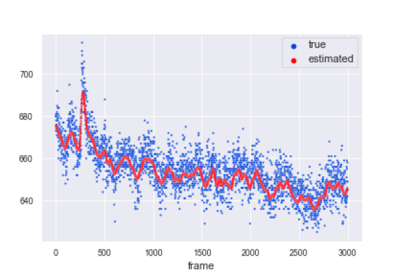
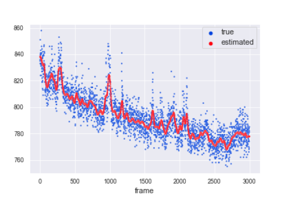
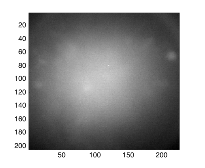
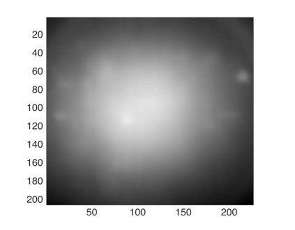
Figure 3: (a) Fitted value for a fixed voxel of coordinate (200,60) over frames (b) Fitted value for a fixed voxel of coordinate (60,180) over frames (c) Original 1500th frame (d) Estimated 1500th frame by our method. This figure appears in color in the electronic version of this article, and any mention of color refers to that version.

Figure 3(a)(b) give estimated fluorescent intensities versus true values of two randomly selected pixels across 3000 frames. The optimal bandwidth and regularization parameter are selected by the proposed BIC criteria. The average rank selected by our method is 22.34 (SE=1.34) across all frames. We also plot estimated images from a randomly selected frame by our method in Figure 3(d). From that figure, we can see that our method amplifies potential neuron signals, but also weakens those unclear and smaller neurons.

We further evaluate the prediction performance of our method by cross-validation. We compare our method with two nonparametric regression methods: Nadaraya-Watson regression and Lasso defined in (3) and (9), respectively. We also compare our method with the low-rank matrix response linear regression (L2RM) method (Kong et al., 2020). The leave-one-out cross-validation error for our method is 2.66 (SE = .63), 2.91 (SE = 1.04) for NW estimator, 2.91 (SE = 1.04) for Lasso estimator, and 5.45 (SE = 3.63) for L2RM. It is clear that our method reaches the smallest leave-one-out cross-validation error among four methods. For Lasso estimator, the selected tuning parameter is always zero, hence making the Lasso estimator equivalent to the Nadaraya-Watson estimator. This confirms that the sparsity assumption does not seem plausible for the calcium imaging application, while low rankness is a more reasonable assumption. The linear model L2RM has the highest prediction error, which validates the use of a nonparametric model for the data set.

6.2 Application to EEG data study

We also apply our method to an EEG dataset that was collected from 122 subjects by the Neurodynamics Laboratory to examine the EEG correlates of genetic predisposition to alcoholism. More details about the study can be found in Zhang et al. (1995). Among the 122 subjects, 77 were alcoholic individuals and 45 were controls. The dataset included voltage values from 64 electrodes placed on each subject’s scalps sampled at 256 Hz (3.9- msec epoch) for 1 second. Each subject was exposed to three stimuli: a single stimulus, two matched stimuli, two unmatched stimuli. For each subject, we use the average of all trials for each subject under single-stimulus condition, which results in a $256\times 64$ matrix. Among those 122 subjects, we randomly select one alcoholic individual and one control, and analyze the dynamic functional connectivity among different electrodes across time. The simplest analytical strategy to investigate dynamic functional connectivity consists in segmenting the time courses from spatial locations into a set of temporal windows, inside which their pairwise connectivity is probed. By gathering functional connectivity descriptive measures over subsequent windows, fluctuations in connectivity can be captured. The basic sliding window framework has been applied by the neuroimaging community to understand how brain dynamics that are related to our cognitive abilities (Kucyi and Davis, 2014; Madhyastha and Grabowski, 2014), is affected by brain disorders (Sakoğlu et al., 2010; Jones et al., 2012), or compares to other functional or structural brain measures (Leonardi et al., 2013; Tagliazucchi et al., 2012; Liégeois et al., 2016). More specifically, we use a moving window of size 100 to calculate a series of covariance matrices along dimension of 256, resulting 157 covariance matrices of size $64\times 64$ for each individual.

We apply the proposed method to analyze the dynamic change of covariance structures over the time in both alcoholic individual and control. In other words, the matrix responses of interest are the dynamic covariance matrices representing the dynamic functional connectivity. The optimal bandwidth and regularization parameter are selected by BIC. Figure 4 shows estimated images of 10th frame by our method for alcoholic individual and control respectively. We observe a significant structural difference in their covariance matrices. Specifically, the alcoholic individual has a more complex covariance structure than that from the control. Moreover, the average selected rank of alcoholic individual is 22.44 (SE = 0.93) compared to 6.82 (SE = 0.87) of control. This can be explained by drastic fluctuation across time in EEG signals of alcoholic individuals compared to stable variation in control. We further evaluate our method by leave-one-out cross-validation error and compare it with Nadaraya-Watson regression, Lasso and L2RM. As shown in Table 2, our method achieves the smallest leave-one-out cross-validation error among three methods. For Lasso estimator, the selected tuning parameter is always zero. In other words, the Lasso estimator is the same as the Nadaraya-Watson estimator for this data application, which implies that the low rankness assumption is a more reasonable assumption than sparsity. We also notice that linear L2RM has a much higher estimation error than the nonparametric methods. This indicates a strong nonlinear pattern in EEG signals for both alcoholic and control subjects.

Table 2: Leave-one-out cross-validation errors (SE) by three methods for EEG data

	Err - Our method	Err - NW	Err - Lasso	Err - L2RM
Alcoholic	1.05 (.008)	2.20 (.018)	2.20 (.018)	908.29 (3.97)
Control	9.57 (.391)	21.87 (.75)	21.87 (.75)	22513.17 (106.78)

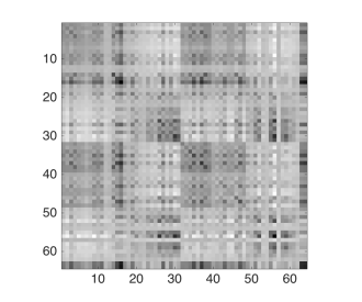
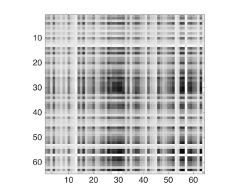
Figure 4: (a) Estimated 10th frame for alcoholic (b) Estimated 10th frame for control

7 Discussion

In this paper, we propose a novel nonparametric matrix response regression model to characterize the nonlinear association between a matrix response and scalar predictors. We introduce a low-rank nonparametric estimation procedure with a computationally efficient algorithm. The applications to the calcium imaging study and the electroencephalography study show superior performance of the proposed approach. Our method has wide applications to other modalities of imaging data as well. For example, one can model the dynamic functional connectivity matrices obtained from resting state or task-evoked fMRI time series. One can also apply our method to characterize the dynamic changes of the 2D brain surface data preprocessed from the MRI data (e.g. hippocampal morphometry surface measure studied in Li et al. (2007); Yu et al. (2020)).

One of the main merits of our method is that our nonparametric estimator has a closed-form solution, and thus makes it computationally fast when analyzing large-scale imaging data. However, there are also several drawbacks. First, our method can only deal with low dimensional covariates. When the dimension of the covariates becomes high, it suffers from the curse of dimensionality, which is a long-standing issue in nonparametric smoothing methods. Second, our method is based on the Nadaraya-Watson estimator, and therefore it may also suffer from poor bias at the boundaries of the domain. To solve this problem, one may incorporate the low-rank estimation procedure into the local linear kernel method. However, the trade-off is that it significantly increases the computational burden as one can not find a closed form solution for the estimator.

There are a number of important directions for future work. First, we model the dynamic functional connectivity as covariance matrices. One can also model them as dynamic network (Nie et al., 2017; Zhang and Cao, 2017) and consider the nonparametric regression for dynamic network. Second, one may also model the images as 2D functional data and study various models to characterize the time-dependence structures among the functional data objects (Zhang and Shao, 2015; Gao et al., 2020).

Data Availability Statement

The data that support the findings in this paper are available in Begleiter (1999) at https://archive.ics.uci.edu/ml/datasets/EEG+Database and Witten (2018) at https://ajpete.com/software/.

Supporting Information

Web Appendices, Tables, computational code, and a sample data set referenced in Sections 3,4, 5, and 6 are available with this paper at the Biometrics website on Wiley Online Library.

References

- Andilla and Hamprecht (2014) Andilla, F. D. and Hamprecht, F. A. (2014). Sparse space-time deconvolution for calcium image analysis. In Advances in Neural Information Processing Systems, pages 64–72.
- Apthorpe et al. (2016) Apthorpe, N., Riordan, A., Aguilar, R., Homann, J., Gu, Y., Tank, D., et al. (2016). Automatic neuron detection in calcium imaging data using convolutional networks. In Advances in Neural Information Processing Systems, pages 3270–3278.
- Begleiter (1999) Begleiter, H. (1999). EEG dataset. https://archive.ics.uci.edu/ml/datasets/EEG+Database (accessed 08/22/2020) .
- Berridge (1998) Berridge, M. J. (1998). Neuronal calcium signaling. Neuron 21, 13–26.
- Biswal et al. (1995) Biswal, B., Zerrin Yetkin, F., Haughton, V. M., and Hyde, J. S. (1995). Functional connectivity in the motor cortex of resting human brain using echo-planar MRI. Magnetic Resonance in Medicine 34, 537–541.
- Biswal et al. (2010) Biswal, B. B., Mennes, M., Zuo, X.-N., Gohel, S., Kelly, C., Smith, S. M., et al. (2010). Toward discovery science of human brain function. Proceedings of the National Academy of Sciences 107, 4734–4739.
- Cai et al. (2010) Cai, J.-F., Candès, E. J., and Shen, Z. (2010). A singular value thresholding algorithm for matrix completion. SIAM Journal on Optimization 20, 1956–1982.
- Calhoun and Adali (2016) Calhoun, V. D. and Adali, T. (2016). Time-varying brain connectivity in fMRI data: whole-brain data-driven approaches for capturing and characterizing dynamic states. IEEE Signal Processing Magazine 33, 52–66.
- Calhoun et al. (2014) Calhoun, V. D., Miller, R., Pearlson, G., and Adalı, T. (2014). The chronnectome: time-varying connectivity networks as the next frontier in fMRI data discovery. Neuron 84, 262–274.
- Chang et al. (2013) Chang, C., Liu, Z., Chen, M. C., Liu, X., and Duyn, J. H. (2013). EEG correlates of time-varying bold functional connectivity. NeuroImage 72, 227–236.
- Chen et al. (2013) Chen, K., Dong, H., and Chan, K.-S. (2013). Reduced rank regression via adaptive nuclear norm penalization. Biometrika 100, 901–920.
- Damaraju et al. (2014) Damaraju, E., Allen, E. A., Belger, A., Ford, J. M., McEwen, S., Mathalon, D., et al. (2014). Dynamic functional connectivity analysis reveals transient states of dysconnectivity in schizophrenia. NeuroImage: Clinical 5, 298–308.
- Dawid (1981) Dawid, A. P. (1981). Some matrix-variate distribution theory: notational considerations and a Bayesian application. Biometrika 68, 265–274.
- De Munck et al. (2002) De Munck, J. C., Huizenga, H. M., Waldorp, L. J., and Heethaar, R. (2002). Estimating stationary dipoles from MEG/EEG data contaminated with spatially and temporally correlated background noise. IEEE Transactions on Signal Processing 50, 1565–1572.
- Ding and Cook (2018) Ding, S. and Cook, D. (2018). Matrix variate regressions and envelope models. Journal of the Royal Statistical Society: Series B (Statistical Methodology) 80, 387–408.
- Engels et al. (2018) Engels, G., Vlaar, A., McCoy, B., Scherder, E., and Douw, L. (2018). Dynamic functional connectivity and symptoms of parkinson’s disease: a resting-state fmri study. Frontiers in Aging Neuroscience 10, 388.
- Fox et al. (2005) Fox, M. D., Snyder, A. Z., Vincent, J. L., Corbetta, M., Van Essen, D. C., and Raichle, M. E. (2005). The human brain is intrinsically organized into dynamic, anticorrelated functional networks. Proceedings of the National Academy of Sciences 102, 9673–9678.
- Friston (1994) Friston, K. J. (1994). Functional and effective connectivity in neuroimaging: a synthesis. Human Brain Mapping 2, 56–78.
- Gao et al. (2020) Gao, X., Shen, W., Shahbaba, B., Fortin, N., and Ombao, H. (2020). Evolutionary state-space model and its application to time-frequency analysis of local field potentials. Statistica Sinica 30, 1561–1582.
- Gao et al. (2020) Gao, X., Shen, W., Zhang, L., Hu, J., Fortin, N. J., Frostig, R. D., and Ombao, H. (2020). Regularized matrix data clustering and its application to image analysis. Biometrics .
- Grienberger and Konnerth (2012) Grienberger, C. and Konnerth, A. (2012). Imaging calcium in neurons. Neuron 73, 862–885.
- Gu et al. (2014) Gu, S., Zhang, L., Zuo, W., and Feng, X. (2014). Weighted nuclear norm minimization with application to image denoising. In Proceedings of the IEEE Conference on Computer Vision and Pattern Recognition, pages 2862–2869.
- Helmchen and Denk (2005) Helmchen, F. and Denk, W. (2005). Deep tissue two-photon microscopy. Nature Methods 2, 932.
- Horwitz (2003) Horwitz, B. (2003). The elusive concept of brain connectivity. NeuroImage 19, 466–470.
- Hu et al. (2020) Hu, W., Shen, W., Zhou, H., and Kong, D. (2020). Matrix linear discriminant analysis. Technometrics 62, 196–205.
- Jones et al. (2012) Jones, D. T., Vemuri, P., Murphy, M. C., Gunter, J. L., Senjem, M. L., Machulda, M. M., et al. (2012). Non-stationarity in the “resting brain’s” modular architecture. PLOS ONE 7, e39731.
- Kong et al. (2020) Kong, D., An, B., Zhang, J., and Zhu, H. (2020). L2RM: Low-rank linear regression models for high-dimensional matrix responses. Journal of the American Statistical Association 115, 403–424.
- Kucyi and Davis (2014) Kucyi, A. and Davis, K. D. (2014). Dynamic functional connectivity of the default mode network tracks daydreaming. NeuroImage 100, 471–480.
- Leonardi et al. (2013) Leonardi, N., Richiardi, J., Gschwind, M., Simioni, S., Annoni, J.-M., Schluep, M., et al. (2013). Principal components of functional connectivity: a new approach to study dynamic brain connectivity during rest. NeuroImage 83, 937–950.
- Li and Zhang (2017) Li, L. and Zhang, X. (2017). Parsimonious tensor response regression. Journal of the American Statistical Association 112, 1131–1146.
- Li et al. (2007) Li, S., Shi, F., Pu, F., Li, X., Jiang, T., Xie, S., and Wang, Y. (2007). Hippocampal shape analysis of alzheimer disease based on machine learning methods. American Journal of Neuroradiology 28, 1339–1345.
- Liégeois et al. (2016) Liégeois, R., Ziegler, E., Phillips, C., Geurts, P., Gómez, F., Bahri, M. A., et al. (2016). Cerebral functional connectivity periodically (de) synchronizes with anatomical constraints. Brain Structure and Function 221, 2985–2997.
- Madhyastha and Grabowski (2014) Madhyastha, T. M. and Grabowski, T. J. (2014). Age-related differences in the dynamic architecture of intrinsic networks. Brain Connectivity 4, 231–241.
- Mao et al. (2001) Mao, B.-Q., Hamzei-Sichani, F., Aronov, D., Froemke, R. C., and Yuste, R. (2001). Dynamics of spontaneous activity in neocortical slices. Neuron 32, 883–898.
- Nie et al. (2017) Nie, Y., Wang, L., and Cao, J. (2017). Estimating time-varying directed gene regulation networks. Biometrics 73, 1231–1242.
- Niu et al. (2019) Niu, H., Zhu, Z., Wang, M., Li, X., Yuan, Z., Sun, Y., et al. (2019). Abnormal dynamic functional connectivity and brain states in alzheimer’s diseases: functional near-infrared spectroscopy study. Neurophotonics 6, 025010.
- Petersen et al. (2018) Petersen, A., Simon, N., and Witten, D. (2018). Scalpel: Extracting neurons from calcium imaging data. The Annals of Applied Statistics 12, 2430.
- Pnevmatikakis et al. (2012) Pnevmatikakis, E. A., Kelleher, K., Chen, R., Saggau, P., Josic, K., and Paninski, L. (2012). Fast spatiotemporal smoothing of calcium measurements in dendritic trees. PLoS Computational Biology 8, e1002569.
- Preti et al. (2017) Preti, M. G., Bolton, T. A., and Van De Ville, D. (2017). The dynamic functional connectome: State-of-the-art and perspectives. NeuroImage 160, 41–54.
- Rahmati et al. (2016) Rahmati, V., Kirmse, K., Marković, D., Holthoff, K., and Kiebel, S. J. (2016). Inferring neuronal dynamics from calcium imaging data using biophysical models and bayesian inference. PLoS Computational Biology 12, e1004736.
- Sakoğlu et al. (2010) Sakoğlu, Ü., Pearlson, G. D., Kiehl, K. A., Wang, Y. M., Michael, A. M., and Calhoun, V. D. (2010). A method for evaluating dynamic functional network connectivity and task-modulation: application to schizophrenia. Magnetic Resonance Materials in Physics, Biology and Medicine 23, 351–366.
- Scott (2015) Scott, D. W. (2015). Multivariate density estimation: theory, practice, and visualization. John Wiley & Sons.
- Stosiek et al. (2003) Stosiek, C., Garaschuk, O., Holthoff, K., and Konnerth, A. (2003). In vivo two-photon calcium imaging of neuronal networks. Proceedings of the National Academy of Sciences 100, 7319–7324.
- Tagliazucchi et al. (2012) Tagliazucchi, E., Von Wegner, F., Morzelewski, A., Brodbeck, V., and Laufs, H. (2012). Dynamic bold functional connectivity in humans and its electrophysiological correlates. Frontiers in Human Neuroscience 6,.
- Tsien and Tsien (1990) Tsien, R. W. and Tsien, R. Y. (1990). Calcium channels, stores, and oscillations. Annual Review of Cell Biology 6, 715–760.
- Wang and Zhu (2017) Wang, X. and Zhu, H. (2017). Generalized scalar-on-image regression models via total variation. Journal of the American Statistical Association 112, 1156–1168.
- Witten (2018) Witten, I. (2018). One-photon calcium imaging dataset. https://ajpete.com/software/ (accessed 08/22/2020) .
- Yu et al. (2020) Yu, D., Wang, L., Kong, D., and Zhu, H. (2020). Beyond scalar treatment: A causal analysis of hippocampal atrophy on behavioral deficits in Alzheimer’s studies. arXiv preprint arXiv:2007.04558 .
- Zhang and Cao (2017) Zhang, J. and Cao, J. (2017). Finding common modules in a time-varying network with application to the drosophila melanogaster gene regulation network. Journal of the American Statistical Association 112, 994–1008.
- Zhang et al. (2016) Zhang, T., Shen, H., and Li, F. (2016). Linear and non-linear models for fmri time series analysis. Handbook of Neuroimaging Data Analysis page 309.
- Zhang and Li (2017) Zhang, X. and Li, L. (2017). Tensor envelope partial least-squares regression. Technometrics 59, 426–436.
- Zhang and Shao (2015) Zhang, X. and Shao, X. (2015). Two sample inference for the second-order property of temporally dependent functional data. Bernoulli 21, 909–929.
- Zhang et al. (1995) Zhang, X. L., Begleiter, H., Porjesz, B., Wang, W., and Litke, A. (1995). Event related potentials during object recognition tasks. Brain Research Bulletin 38, 531–538.
- Zhang et al. (2020) Zhang, Y., Shen, W., and Kong, D. (2020). Covariance estimation for matrix-valued data. arXiv preprint arXiv:2004.05281 .
- Zhou and Li (2014) Zhou, H. and Li, L. (2014). Regularized matrix regression. Journal of the Royal Statistical Society: Series B (Statistical Methodology) 76, 463–483.
- Zhu et al. (2019) Zhu, H., Huang, J., Deng, L., He, N., Cheng, L., Shu, P., et al. (2019). Abnormal dynamic functional connectivity associated with subcortical networks in parkinson’s disease: A temporal variability perspective. Frontiers in Neuroscience 13, 80.
- Zhu et al. (2011) Zhu, H., Kong, L., Li, R., Styner, M., Gerig, G., Lin, W., and Gilmore, J. H. (2011). FADTTS: functional analysis of diffusion tensor tract statistics. NeuroImage 56, 1412–1425.
- Zhu et al. (2012) Zhu, H., Li, R., and Kong, L. (2012). Multivariate varying coefficient model for functional responses. Annals of Statistics 40, 2634.