Game of Variable Contributions to the Common Good under Uncertainty

Abstract

We consider a stochastic game of contribution to the common good in which the players have continuous control over the degree of contribution, and we examine the gradualism arising from the free rider effect. This game belongs to the class of variable concession games which generalize wars of attrition. Previously known examples of variable concession games in the literature yield equilibria characterized by singular control strategies without any delay of concession. However, these no-delay equilibria are in contrast to mixed strategy equilibria of canonical wars of attrition in which each player delays concession by a randomized time. We find that a variable contribution game with a single state variable, which extends the Nerlove-Arrow model, possesses an equilibrium characterized by regular control strategies that result in a gradual concession. This equilibrium naturally generalizes the mixed strategy equilibria from the canonical wars of attrition. Stochasticity of the problem accentuates the qualitative difference between a singular control solution and a regular control equilibrium solution. We also find that asymmetry between the players can mitigate the inefficiency caused by the gradualism.
Keywords: Nerlove-Arrow model, war of attrition, stochastic control game, free rider problem, gradualism

1 Introduction

Many business or public policy decisions concern the free rider problem when contributing to a stock of common good. (Hardin, 1968). It is well-known that a free rider problem induces a wait and see approach of the individuals who are in a position to contribute to the common good (Tirole, 2017). The wait and see approach in turn results in underinvestment in the common good. Hence, it is important for decision makers and social planners to understand the game-theoretic implications of the free rider problem involving the common good. Industry examples of a free rider problem with the common good can be found in the context of generic advertisement for commodities. For instance, the advertising expenditures by Florida orange juice advertising programs not only benefit the Florida orange juice industry, but it also benefits non-Florida orange juice importers (Lee and Fairchild, 1988). In another example, it has been shown that a salmon promotion program conducted by Norway has benefited its international competitors, too (Kinnucan and Myrland, 2003). In these examples, the advertising expenditures of one agent contribute to the stock of the product’s overall goodwill, “which summarizes the effects of current and past advertising outlays on demand” (Nerlove and Arrow, 1962). The stock of goodwill is the common good in the context of generic advertising because it benefits other agents, even if they do not contribute to it. In this paper, we examine the game of variable contribution to the common good where the stock of common good evolves stochastically. In particular, we obtain the free rider effect on its Markov perfect equilibrium (MPE) and compare and contrast it to other games of concession. We address the question of whether the equilibrium suffers from the gradualism of the players’ contributions to the common good and, if so, whether the inefficiency arising from the gradualism can be mitigated.

One objective of the paper is to fill the gaps in the equilibrium characteristics of variable concession games in which the cost is linear in the contribution. The problem of contribution to common good belongs to the class of variable concession games in which the players can control the degree of concession. This class of games constitutes a significant generalization of the war of attrition. In the canonical war of attrition, each player can either continue the game or concede completely, and it typically yields a mixed strategy equilibrium in which the players delay their concession by a randomized time. The central question of this paper concerns the characteristics of the variable concession games. We can imagine three possibilities of equilibrium strategies: (1) singular control (lump-sum contribution) strategies without time delay, (2) singular control strategies with time delay, and (3) regular control strategies that lead to an equilibrium characterized by gradualism. In the current literature, the variable concession games thus far have resulted in type (1) equilibrium with singular control strategies of immediate lump-sum concession. Type (2), if it exists, is closest to the mixed strategy equilibrium of the war of attrition, but it has not been found in the literature or in this paper. The other natural generalization of the mixed strategy time delay equilibrium to variable concession games is type (3), which has yet to be found in the current literature on variable concession games with linear cost. Our paper shows that type (3) is found in a very simple game-theoretic and stochastic extension of the Nerlove-Arrow model of goodwill stock (Nerlove and Arrow, 1962; Sethi, 1977; Lon and Zervos, 2011).

In our model, two players are considering irreversible and costly contribution to the stock of common good. Each player can contribute any amount to the common good at any point in time, but the common good increases the flow profit to both players. The stock of common good evolves stochastically, and it tends to decline in time on average unless someone contributes to it, just as the stock of goodwill for a product depreciates in time without advertisement (Nerlove and Arrow, 1962). In this game, the strategy of each player is represented by the dynamic path of its cumulative contribution. We formulate the problem as a stochastic control game and utilize the well-established stochastic control theory. In order to find the equilibrium, we need to obtain the best responses, so we establish the verification theorem for the best response stochastic control.

This paper has three main contributions. First, we show that the model that we consider has a gradualist equilibrium characterized by regular control. This result is in contrast to the typical control solution: in a control problem with a linear cost structure, the single decision maker solution is characterized by singular control rather than regular control. Second, we find that stochasticity and asymmetry have significant impact on the equilibrium characteristics. In the deterministic game, both the singular control solution and the equilibrium solution exhibit a stable steady state so that an outsider may not be able to tell the difference between the two. In contrast, in the stochastic case, the two solutions exhibit markedly different behavior and are easier to observe in the empirical sense. We also find that asymmetry between the players destabilizes the gradualist equilibrium, and the outcome is an asymmetric equilibrium with singular control strategy adopted by at least one of the players. Hence, asymmetry can mitigate the inefficiency of the gradualist equilibrium. Third, the paper provides a mathematical framework to obtain an MPE of a stochastic game of variable concession involving both singular and regular control.

Although there are many equilibrium solution concepts, we limit our attention to MPE (Maskin and Tirole, 2001). MPE is a subgame perfect equilibrium in which the players’ actions are determined by the current value, but not by the past history, of the economically relevant state variable, and hence it is a key notion for analyzing a game.

Cooperative equilibrium concepts are beyond the scope of this paper. Coordinated plans of action do produce an efficient outcome, which will change the form of the solution; for instance, the singular control boundary will change. Although cooperation does happen between contributors to common good, it often requires prior coordination or bargaining, and we can still consider the non-cooperative MPE a baseline solution prior to coordination. For instance, in a Nash bargaining solution (Nash, 1950), the non-cooperative MPE outcome can serve as the disagreement point, and therefore, it is still a meaningful reference point.

The paper contributes to the literature on variable concession games, which an extension of a war of attrition (Maynard Smith, 1974). Typical attrition games under complete information possess mixed strategy equilibria with random time delays, both in the deterministic case (Hendricks et al., 1988) and in the stochastic case (Steg, 2015; Georgiadis et al., 2019). In contrast, the known examples of the game of variable concession exhibit singular control equilibria with no time delay. One example is Cournot competition under declining demand when the firms can reduce the production capacity at a variable cost (Ghemawat and Nalebuff, 1990). The equilibrium strategy is to immediately reduce the capacity to the myopic Cournot equilibrium level through singular control. The stochastic generalization of the Cournot model also exhibits similar characteristics (Steg, 2012).

The paper also contributes to the literature on games of contribution to public goods. Fershtman and Nitzan (1991) examine a dynamic game of voluntary contribution to public goods. In their model, players continuously contribute to the stock of public goods over time. They obtain an equilibrium using a differential game approach and demonstrate that the free riding problem is acute without commitment. Their model is similar to ours, but they model a situation with costs that grow quadratically with the rate of contribution, so it is prohibitively costly to make a lump sum contribution. Since our model allows for a lump sum contribution due to the linear cost structure, the characteristics of the equilibria are very different, and it is difficult to compare their results to ours. Battaglini et al. (2014) examine a problem of dynamic free riding in which each individual allocates its endowment between private consumption and irreversible contribution to the public good. They study the implications of the irreversibility of their model and conclude that irreversibility can alleviate inefficiency of the equilibria. It is noteworthy that the equilibrium of their model involves lump sum contribution (singular control) strategies. Ferrari et al. (2017) examine a significantly generalized model with stochasticity to obtain its equilibria and study the effect of uncertainty and irreversibility of contribution to the public good. They also obtain equilibria characterized by lump sum contribution strategies. In contrast to the literature on private consumption and contribution to the public good, our model does not incorporate consumption of the players.

Because our model assumes that the cost of contribution is linear in the magnitude of the improvement in the common good, we formulate it as a game-theoretic extension of monotone follower singular control problems with a single dimensional state variable. In a similar vein, Lon and Zervos (2011) apply singular control framework to the Nerlove-Arrow model of expenditure in the stock of goodwill. Recently, some work on game-theoretic study of singular control problems has emerged. Steg (2012) examines Cournot competition that leads to a singular control equilibrium. Kwon and Zhang (2015) examines a singular control game in the context of a market share competition in which a player’s control is to negate his opponent’s payoff. Ferrari et al. (2017) also analyze a model that incorporates game-theoretic singular control, but the model has a more complex structure as the players make consumption and contribution decisions at the same time.

The paper is organized as follows. In Section 2, we examine a game of variable contribution to the common good and show that it yields a regular control strategy equilibrium. In Section 3, we examine the impact of stochasticity and asymmetry between the players. In particular, we show that asymmetry eliminates the regular control equilibrium thereby improving the efficiency. In Section 4, we discuss several aspects of the results that are worthy of note. In Section 5, we summarize the main results and implications of the paper and provide concluding remarks.

2 Variable Contribution Game

In this section, we present a game of variable contribution to the common good that results in a regular control equilibrium. We first present the model in Section 2.1, and then we examine the single decision maker case as a benchmark in Section 2.2. We construct the verification theorem for best responses in Section 2.3 and obtain the regular control MPE in Section 2.4.

2.1 The Model

We consider a game between two players, each of whom receives a flow profit that depends on a common state variable. Either player can boost the common state variable at a cost by any amount at any point in time. The model is applicable to a number of industry examples. One example is a game between two manufacturers who share a common supplier. Each manufacturer can make a variable investment to boost the quality of the shared supplier, which in turn benefits the other manufacturer through spillover (Muthulingam and Agrawal, 2016; Kim et al., 2017). Another example is the game of irreversible and variable investment in the stock of goodwill (Nerlove and Arrow, 1962) through advertisement such as in generic advertising on commodities (Lee and Fairchild, 1988; Kinnucan and Myrland, 2003).

We let the process $Z=\{Z_{t}:t\geq 0\}$ denote the stock of common good defined in the interval $I=(a,b)\subseteq\mathbb{R}$ on a filtered probability space $(\Omega,\mathcal{F},\mathcal{F}_{t},\mathbb{P})$ that satisfies the usual condition. If $I=\mathbb{R}$, for example, it is understood that $a=-\infty$ and $b=\infty$. We assume that $Z$ satisfies the following stochastic differential equation (SDE):

$$dZ_{t}=\mu(Z_{t})dt+\sigma(Z_{t})dW_{t}+d\xi_{it}+d\xi_{jt}\;,$$

where $W=\{W_{t}:t\geq 0\}$ is a Wiener process progressively measurable with respect to $\{\mathcal{F}_{t}:t\geq 0\}$. Here $\mu(\cdot)$ is the drift term which we interpret as the time-averaged rate of change of $Z$ in the absence of control. In this paper, we assume $\mu(\cdot)<0$ to model the deterioration of the common good. The volatility $\sigma(\cdot)>0$ represents the magnitude of the white noise. The process $\xi_{i}=\{\xi_{it}:t\geq 0\}$ is a non-decreasing càdlàg (right continuous with left limits) process controlled by player $i$ adapted to $\{\mathcal{F}_{t}:t\geq 0\}$. We interpret $\xi_{it}$ as the cumulative contribution of player $i$ to $Z$ up to time $t$. Since each player $i$ controls the process $\xi_{i}$, we say that $\xi_{i}$ is player $i$’s strategy, and $\xi=(\xi_{i},\xi_{j})$ is the strategy profile. Throughout the paper, we let $\Xi_{i}$ denote the set of all possible $\mathcal{F}_{t}$-adapted control processes $\xi_{i}$.

We remark that $\xi_{i}$ is composed of a continuous process and a discontinuous process as follows:

$$\xi_{it_{2}}-\xi_{it_{1}^{-}}=\int_{t_{1}}^{t_{2}}d\xi_{it}^{c}+\sum_{t\in[t_{1},t_{2}]}\Delta\xi_{it}\>,$$

where $\xi_{i}^{c}$ is the continuous part of $\xi_{i}$, and $\Delta\xi_{it}=\xi_{it}-\xi_{it^{-}}$ is the instantaneous jump in $\xi_{i}$ at time $t$. Similarly, we can decompose the process $Z_{t}$ into a continuous part $Z_{t}^{c}$ and a discontinuous part $\Delta Z_{t}=Z_{t}-Z_{t^{-}}=\Delta\xi_{1t}+\Delta\xi_{2t}$.

Given a strategy profile $\xi$, player $i$’s payoff is given by the following function:

$$V_{i}(x;\xi)=\mathbb{E}^{x}\left[\int_{0}^{\infty}e^{-rt}\pi_{i}(Z_{t})dt-\int_{0}^{\infty}e^{-rt}k_{i}d\xi_{it}\right]\>.$$

Here $\mathbb{E}^{x}[\cdot]=\mathbb{E}[\cdot|Z_{0}=x]$ is the conditional expectation operator given the initial condition $Z_{0}=x$. The integrand $\pi_{i}(\cdot)$ is a non-decreasing function that represents the profit flow for player $i$, and $k_{i}>0$ is the cost of increasing a unit of $\xi_{i}$. Lastly, $r>0$ is the discount rate common to both players.

For the sake of analytical tractability, we make a number of assumptions below that are standard in the stochastic control literature. We first make some assumptions regarding $\mu(\cdot)$ and $\sigma(\cdot)$. Let $X=\{X_{t}\,:\,t\geq 0\}$ denote the uncontrolled process which satisfies $dX_{t}=\mu(X_{t})dt+\sigma(X_{t})dW_{t}$.

Assumption 1

(i) $\mu(\cdot)$ and $\sigma(\cdot)$ are Lipschitz continuous functions satisfying $|\mu(x)|+|\sigma(x)|\leq\delta(1+|x|)$ for some constant $\delta>0$.

(ii) $\{e^{-r\tau}(X_{t})^{-}:\text{$\tau\ $}\text{is a stopping time},\;\tau<\infty\}$ is uniformly integrable for any initial value $X_{0}=x$. Furthermore, $\lim_{t\rightarrow\infty}\mathbb{E}^{x}[e^{-rt}(X_{t})^{-}]=0$.

Assumption 1 (i) implies that the uncontrolled process $X$ has a unique strong solution to the SDE. It also implies that $\sigma(\cdot)$ is locally bounded; this will be useful when we apply Dynkin’s formula to the payoff function because the stochastic integral involving $\sigma(Z_{t})dW_{t}$ is a local martingale which possesses convenient properties (Chapter IV, Revuz and Yor, 1999). Assumption 1 (ii) ensures that the limiting behaviors of the process $X$ are well-defined so that we can construct a verification theorem in Section 2.3.

Below we let $C(I)$ denote the set of continuous functions defined on $I$.

Assumption 2

$\pi_{i}(\cdot)\in C(I)$ is strictly increasing and bounded from above, i.e., $\lim_{x\rightarrow b}\pi_{i}(x)<\pi_{M}$ for some positive constant $\pi_{M}$. Furthermore, it satisfies the absolute integrability condition $\mathbb{E}^{x}\left[\int_{0}^{\infty}\left|e^{-rt}\pi_{i}(X_{t})\right|dt\right]<\infty$ for the uncontrolled process $X$.

Assumption 2 ensures that the payoff $V_{i}(x;\xi)$ is well-defined and that the function

$$(R\pi_{i})(x):=\mathbb{E}^{x}\left[\int_{0}^{\infty}e^{-rt}\pi_{i}(X_{t}^{x})dt\right]$$ (2.1)

exists. The function $(R\pi_{i})(\cdot)$ has the meaning of the payoff from perpetually keeping an uncontrolled process $X$. Later we establish that $(R\pi_{i})(\cdot)$ is an element of the payoff function.

Next, we define the $r$-excessive characteristic operator (Alvarez, 2003):

$$\mathcal{A}:=\frac{1}{2}\sigma(x)^{2}\partial_{x}^{2}+\mu(x)\partial_{x}-r\>.$$ (2.2)

We let $\psi(\cdot)$ and $\phi(\cdot)$ respectively denote two linearly independent increasing and decreasing fundamental solutions to the differential equation $\mathcal{A}\psi(x)=\mathcal{A}\phi(x)=0$ (Borodin and Salminen, 1996; Alvarez, 2003). We remark that $(R\pi_{i})(\cdot)$ satisfies the differential equation $\mathcal{A}(R\pi_{i})(x)+\pi_{i}(x)=0$ according to the optimal stopping theory.

We also define the following functions

$$q_{i}(x) =\pi_{i}(x)+\mathcal{A}k_{i}x=\pi_{i}(x)+[\mu(x)-rx]k_{i}\;,$$ (2.3)

$$(Rq_{i})(x) =\mathbb{E}^{x}\left[\int_{0}^{\infty}e^{-rt}q_{i}(X_{t})dt\right]\>,$$

and assume the following properties of $(R\pi_{i})(\cdot)$ and $q_{i}(\cdot)$:

Assumption 3

(i) $(R\pi_{i})(\cdot)$ satisfies $\lim_{x\rightarrow a}(R\pi_{i})(x)<0$ and $\lim_{x\rightarrow a}(R\pi_{i})(x)/\phi(x)=0$. (ii) There exists some $x_{i}^{*}\in I$ such that $q_{i}(x)$ is strictly increasing for $x<x^{*}$ and strictly decreasing for $x>x^{*}$. (iii) $\lim_{x\rightarrow a}q(x)=-\infty$, $\lim_{x\rightarrow a}q(x)\psi^{\prime}(x)\exp\left(\int_{0}^{x}\frac{2\mu(y)}{\sigma^{2}(y)}dy\right)=0$, $\lim_{x\rightarrow b}q(x)\phi^{\prime}(x)\exp\left(\int_{0}^{x}\frac{2\mu(y)}{\sigma^{2}(y)}dy\right)=0$, and $\lim_{x\rightarrow b}(Rq)^{\prime}(x)/\phi^{\prime}(x)>0$.

Assumption 3 serves as the sufficient condition for the unique optimal control solution to exist for the model examined in Section 2.2. Specifically, in the single decision maker’s problem, the assumptions drive a solution with a singular control region of the form $(a,\theta)$ for some threshold $\theta$. Assumption 3 (i) ensures that the flow profit function $\pi_{i}(\cdot)$ is negative and well-behaved near $a$. To gain an intuitive understanding of the assumptions regarding $q_{i}(\cdot)$, we consider a special case of $\mu(x)=\mu$, in which case $q_{i}^{\prime}(x)=\pi_{i}^{\prime}(x)-rk_{i}$. Then Assumption 3 (ii) implies that $\pi_{i}^{\prime}(x)>rk_{i}$ for $x<x_{i}^{*}$ and $\pi_{i}^{\prime}(x)<rk_{i}$ for $x>x_{i}^{*}$. This implies that it is optimal to boost $\xi_{i}$ if and only if $x<x_{i}^{*}$. Thus, the players have incentive to boost $\xi_{i}$ only if $X_{t}$ falls below a threshold. Assumption 3 (iii) ensures that a unique threshold for boosting $\xi_{i}$ exists for the model examined in Section 2.2.

2.2 Benchmark: Single Decision Maker Problem

In this subsection, we review the single decision maker problem as a benchmark and provide the optimal solution. This class of problems is extensively examined in the literature (Alvarez, 2001; Øksendal and Sulem, 2005; Lon and Zervos, 2011), but we reproduce it here because its solution will be utilized in the equilibrium solution of the game in the remainder of the paper.

Since there is only one decision maker, we drop the player index $i$ for convenience throughout Section 2.2. The value function associated with a control policy $\xi=\{\xi_{t}:t\geq 0\}$ is given by

$$V(x;\xi)=\mathbb{E}^{x}\left[\int_{0}^{\infty}e^{-rt}\pi(Z_{t})dt-\int_{0}^{\infty}e^{-rt}kd\xi_{t}\right]\>.$$

The objective of the decision maker is to maximize $V(\cdot;\xi)$ with respect to $\xi$. This class of problems is known as the singular stochastic control monotone follower problems.

We first provide the sufficient condition (the optimality condition) for the optimal control solution. We let $C^{n}(I)$ denote the set of functions defined on $I$ that are $n$ times continuously differentiable. Suppose that $V(\cdot)\in C^{2}(I)$ satisfies the following conditions: (i) $\mathcal{A}V(x)+\pi(x)\leq 0$ and $V^{\prime}(x)-k\leq 0$ for all $x\in I$, and (ii) $[\mathcal{A}V(x)+\pi(x)][V^{\prime}(x)-k]=0$ for all $x\in I$. Then $V(x)$ coincides with the optimal solution $\sup_{\xi\in\Xi}V(x;\xi)$. The proof of this sufficient condition is provided, for example, by Øksendal and Sulem (2005) and Lon and Zervos (2011), and so we will not reproduce it here.

Lemma 1

Under Assumptions 1–3, there exist a threshold $\theta\in I$ and a coefficient $A$ such that the optimal solution $V(\cdot)\in C^{2}(I)$ is given as follows:

$$V(x)=\begin{cases}k(x-\theta)+V(\theta)&\text{for}\;x<\theta\\ (R\pi)(x)+A\phi(x)&\text{for}\;x\geq\theta\end{cases}\>.$$ (2.4)

Next, we provide the intuition behind the solution through a numerical example.

Example 1: We consider a problem of constant $\mu(x)=\mu<0$ and $\sigma(x)=\sigma>0$ and the flow profit $\pi(x)=1-\exp(\nu x)$ with $\nu<0$ that satisfies $\frac{1}{2}\sigma^{2}\nu^{2}+\mu\nu-r<0$. Then it is straightforward to verify that $\phi(x)=\exp(\gamma_{-}x)$ and $\psi(x)=\exp(\gamma_{+}x)$ where

$$\gamma_{\pm}=\frac{1}{\sigma^{2}}(-\mu\pm\sqrt{\mu^{2}+2r\sigma^{2}})\>,$$

and

$$(R\pi)(x) =\frac{1}{r}-\frac{\exp(\nu x)}{\beta}\>,$$

$$\text{where }\quad\beta =r-\mu\nu-\frac{1}{2}\sigma^{2}\nu^{2}\>.$$

Assumptions 1–3 are satisfied in this example so that Lemma 1 applies. Furthermore, the optimal threshold $\theta$ and the coefficient are given by

$$\theta =\frac{1}{\nu}\ln\frac{k\beta\gamma_{-}}{\nu(\nu-\gamma_{-})}\;,$$

$$A =\frac{k-(R\pi)^{\prime}(\theta)}{\phi^{\prime}(\theta)}\>.$$

For the numerical illustration in Fig. 1, we set $\mu=-1$, $\sigma=r=k=1$. In this case, $\theta=-4.3605$ is the optimal threshold. See Fig. 1 for a simulated sample path of $Z$ and $\xi$ and the optimal value function $V(x)$.

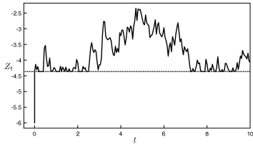
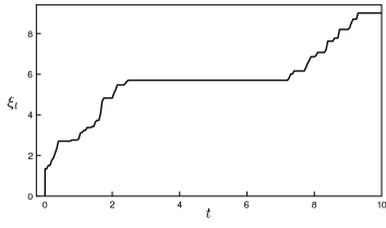
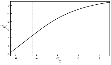
Figure 1: Single decision maker solution. The dotted lines indicate the threshold $\theta$.

The optimal policy associated with the value function (2.4) is a singular control policy: to boost $Z_{t}$ instantaneously up to $\theta$ whenever $Z_{t}$ falls below $\theta$. If the initial value $Z_{0}$ is below $\theta$, then $Z_{t}$ discontinuously jumps to $\theta$ at time $0$, after which $Z_{t}$ is continuous. The threshold $\theta$ functions as a reflecting boundary as shown in Fig. 1. In the region below $\theta$, the value function is linear in $x$ with the slope $k$, as illustrated in the figure as well as expressed in (2.4). This is because $(a,\theta)$ is the singular control region in which it costs exactly $k$ to boost $Z$ by a unit.

2.3 Verification Theorem for Best Responses

Next, we return to the game-theoretic model introduced in the beginning of the section. Our goal is to construct the verification theorem for best responses, which will then be used to construct MPEs in the remainder of the paper.

In a conventional solution to the singular control problem as in Section 2.2, the optimal control process is decomposed as $d\xi_{it}=d\xi_{it}^{l}+\Delta\xi_{it}$ where $\Delta\xi_{it}=\xi_{it}-\xi_{it^{-}}$ represents the discontinuous evolution of the process $\xi_{i}$ while $\xi_{it}^{l}$ is a continuous process like a local time (Protter, 2003). The process $\xi_{it}^{l}$ is not absolutely continuous with respect to Lebesgue measure and cannot be represented as an integral $\int_{0}^{t}u_{is}ds$ for any process $u_{i}=\{u_{it}:t\geq 0\}$ (Karatzas, 1983); for example, the sample path of $\xi$ in Figure 1 does not possess well-defined time derivatives when $\xi_{t}$ increases in time. Both components $\xi_{it}^{l}$ and $\Delta\xi_{it}$ constitute the singular part of $\xi_{it}$. In general, however, a control process must also encompass a regular control process as follows:

$$d\xi_{it}=u_{it}dt+d\xi_{it}^{l}+\Delta\xi_{it}\;,$$

where $u_{it}\geq 0$ is a process adapted to $(\mathcal{F}_{t})$.

To apply the conventional stochastic control theory, we need to define the feasible space of $u_{i}$. More specifically, in order for the SDE $dZ_{t}=\mu(Z_{t})dt+\sigma(Z_{t})dW_{t}+\sum_{i=1}^{2}d\xi_{it}$ to have a unique strong solution, we need to limit $u_{i}$ within the class of $u_{i}(t,x)$ that satisfies the two following conditions: (1) $u_{i}(t,x)$ is Lipschitz continuous in $x$, and (2) $|u_{i}(t,x)|\leq\delta(1+|x|)$ for some constant $\delta$. Let $\mathcal{U}$ be the set of functions $u:(0,\infty)\times I\rightarrow\mathbb{R}$ that satisfy these two conditions. Then we let $\Sigma_{i}$ denote the set of $\mathcal{F}_{t}$-adapted processes $\xi_{it}$ that satisfy $d\xi_{it}=u_{i}(t,Z_{t})dt+d\xi_{it}^{l}+\Delta\xi_{it}$ for some $u_{i}\in\mathcal{U}$. We remark that if $\text{$\xi$}_{i}\in\Sigma_{i}$ then the SDE of $Z$

$$dZ_{t}=[\mu(Z_{t})+\sum_{i=1}^{2}u_{i}(t,Z_{t})]dt+\sigma(Z_{t})dW_{t}+\sum_{i=1}^{2}(d\xi_{it}^{l}+\Delta\xi_{it})$$

satisfies the sufficient condition for possessing a unique strong solution because $u_{i}\in\mathcal{U}$. Note also that $\Sigma_{i}$ is a proper subset of the feasible strategy space $\Xi_{i}$, which is the set of all possible $\mathcal{F}_{t}$-adapted control processes $\xi_{it}$.

Let $\mathcal{M}_{i}$ be the set of player $i$’s Markov control strategies $\xi_{i}$ which depend only on the current value of $Z_{t}$. It means that $\xi_{it}$ satisfies $d\xi_{it}=u_{i}(Z_{t})dt+d\xi_{it}^{l}+\Delta\xi_{it}$ where the singular control region is given as a subset of $I$. For instance, if the singular control region of player $i$ is $[\alpha,\beta]$, then whenever $Z_{t^{-}}\in[\alpha,\beta]$, $\xi$ undergoes a jump $\Delta\xi_{it}=\beta-Z_{t^{-}}$, i.e., player $i$ boosts $Z$ up to $\beta$. Furthermore, $d\xi_{it}^{l}>0$ only when $Z_{t}$ hits $\beta$. By definition, an MPE is a subgame perfect equilibrium $\xi=(\xi_{i},\xi_{j})$ that belongs to $\mathcal{M}_{i}\times\mathcal{M}_{j}$.

For the purpose of obtaining MPE $\xi\in\mathcal{M}_{i}\times\mathcal{M}_{j}$ we can safely focus on obtaining the best response strategies $\xi_{i}^{\prime}\in\Xi_{i}$ in response to the opponent’s Markov strategy $\xi_{j}\in\mathcal{M}_{j}$, i.e., to obtain $\xi_{i}\in\Xi_{i}$ such that $V_{i}(x;\xi_{i},\xi_{j})=\sup_{\xi_{i}^{\prime}\in\Xi_{i}}V_{i}(x;\xi_{i}^{\prime},\xi_{j})$. If the best response $\xi_{i}$ happens to belong to $\mathcal{M}_{i}$, then $\xi=(\xi_{i},\xi_{j})$ is an MPE. Note that we do not, however, look for $\xi_{i}\in\mathcal{M}_{i}$ such that $V_{i}(x;\xi_{i},\xi_{j})=\sup_{\xi_{i}^{\prime}\in\mathcal{M}_{i}}V_{i}(x;\xi_{i}^{\prime},\xi_{j})$; because $\mathcal{M}_{i}\subset\Xi_{i}$, there may be another $\xi_{i}^{\prime}\in\Xi_{i}$ such that $V_{i}(x;\xi_{i}^{\prime},\xi_{j})>V_{i}(x;\xi_{i},\xi_{j})$, in which case $(\xi_{i},\xi_{j})$ is not a Nash equilibrium.

Since we assume a Markov control process $\xi_{j}\in\mathcal{M}_{j}$, we can partition the interval $I$ into regions of discontinuous $\xi_{jt}$ and continuous $\xi_{jt}$. Let $C_{j}$ denote the open subset of $I$ in which $\xi_{jt}$ evolves continuously and non-singularly in time, and let $D_{j}=I\backslash C_{j}$ denote the singular control region where $d\xi_{jt}^{c}>0$ or $\Delta\xi_{jt}>0$.

Now we provide sufficient conditions for the best response to $\xi_{j}$.

Theorem 1

Suppose Assumptions 1–3 hold. Assume player $j$’s Markov strategy $\xi_{j}\in\mathcal{M}_{j}\cap\Sigma_{j}$ that satisfies $d\xi_{jt}=u_{j}(Z_{t})dt+d\xi_{jt}^{l}+\Delta\xi_{jt}$ for some function $u_{j}(\cdot)\geq 0$. Suppose that there exist a function $U(\cdot)$ on $I$ and some Markov strategy $\xi_{i}^{*}\in\mathcal{M}_{i}\cap\Sigma_{i}$ that satisfy the SDE

$$d\xi_{it}^{*}=u_{i}^{*}(Z_{t})dt+d\xi_{it}^{*l}+\Delta\xi_{it}^{*}\>$$ (2.5)

for some $u_{i}^{*}(\cdot)\geq 0$ and the following conditions:

(i) $U(\cdot)\in C^{2}(C_{j})\cap C(I)$, and $U(\cdot)$ is non-decreasing and bounded from above. Furthermore, $U^{\prime}(x)=0$ in the interior of $D_{j}$, and $U^{\prime}(Z_{t})d\xi_{jt}^{l}=0$ for all $t$, where $Z$ is the state process that evolves under the strategy profile $(\xi_{i}^{*},\xi_{j})$.

(ii) There is a function $\tilde{U}(x)\in C^{2}(I)$ such that $\tilde{U}(x)=U(x)$ for all $x\in C_{j}$ and $\tilde{U}^{\prime}(x)$ is bounded for $x\in D_{j}$.

(iii) $\max\{\mathcal{A}U(x)+\pi_{i}(x)+u_{j}(x)U^{\prime}(x)+v_{i}U^{\prime}(x)-v_{i}k_{i},U^{\prime}(x)-k_{i}\}\leq 0$ for all $x\in C_{j}$ and any arbitrary $v_{i}\geq 0$.

(iv) Let $D_{i}=\{x\in I:\Delta\xi_{it}^{*}>0\;\text{whenever}\>x=Z_{t^{-}}\}\cap C_{j}$ be player $i$’s singular control region within $C_{j}$ and $C_{i}=\{x\in I:\Delta\xi_{it}^{*}=0\;\text{whenever}\>x=Z_{t^{-}}\}\cap C_{j}$. Then $\mathcal{A}U(x)+\pi_{i}(x)+u_{j}(x)U^{\prime}(x)+u_{i}^{*}(x)U^{\prime}(x)-u_{i}^{*}(x)k_{i}=0$ for all $x\in C_{i}$ and $U^{\prime}(x)=k_{i}$ for all $x\in D_{i}$.

Then $\xi_{i}^{*}$ is the best response to $\xi_{j}$ amongst all control processes that belong to $\Sigma_{i}$, i.e., $V_{i}(x;\xi_{i}^{*},\xi_{j})=\sup_{\xi_{i}\in\Sigma_{i}}V_{i}(x;\xi_{i},\xi_{j})$.

Remark: Strictly speaking, Theorem 1 does not give sufficient conditions for the best response among the whole strategy space $\Xi_{i}$, but it gives sufficient conditions for the best response among the limited space $\Sigma_{i}$. However, the strategy profiles that we obtain in Theorem 2 and Proposition 1 are proper MPE. This result is obtained because even though Theorem 1 is used to obtain $(\xi_{1},\xi_{2})\in\Sigma_{1}\times\Sigma_{2}$ that satisfies $V_{i}(x;\xi_{i},\xi_{j})=\sup_{\xi_{i}^{\prime}\in\Sigma_{i}}V_{i}(x;\xi_{i}^{\prime},\xi_{j})$ for both $i=1,2$, we can show that

$$V_{i}(x;\xi_{i},\xi_{j})=\sup_{\xi_{i}^{\prime}\in\Xi_{i}}V_{i}(x;\xi_{i}^{\prime},\xi_{j})\;,$$

by the optimality condition for singular control given in Section 2.2. The same is true if $i$ and $j$ are interchanged. Therefore, $(\xi_{1},\xi_{2})$ is a proper MPE. The detail is provided in the proof of Theorem 2.

2.4 Regular Control Strategy Equilibrium

Next, we construct a regular control MPE. We define a regular control MPE as one with control strategies of the following form for both players $i=1,2$:

$$d\xi_{it}=u_{i}(Z_{t})dt\;,$$

where $\xi_{i}\in\Sigma_{i}$. In this subsection, we assume that the two players are symmetric, i.e., $\pi_{i}=\pi_{j}=\pi$ and $k_{i}=k_{j}=k$.

Theorem 2

Suppose Assumptions 1–3 hold. Let $V(\cdot)$ denote the solution (2.4) to the single decision maker problem. Also define a symmetric strategy profile $\xi=(\xi_{1},\xi_{2})$ with the regular control process $d\xi_{it}=u(Z_{t})dt$, where

$$u(x)=\begin{cases}-\frac{1}{k}\left(\mathcal{A}V(x)+\pi(x)\right)&\text{for}\;x<\theta\\ 0&\text{for}\;x\geq\theta\end{cases}\>.$$ (2.6)

Lastly, suppose $u(\cdot)\in\mathcal{U}$. Then $\xi$ is an MPE with a symmetric payoff $V_{i}(x;\xi)=V_{j}(x;\xi)=V(x)$.

Theorem 2 obtains an MPE completely characterized by regular control. Intuitively, both players exert gradual control $u(\cdot)$ if and only if $Z$ is sufficiently low (less than $\theta$). The regular control MPE is reminiscent of the mixed strategy delay equilibrium of the canonical war of attrition in which both players gradually concede in the probabilistic sense through a Poisson process. Thus, we may consider the regular control strategy equilibrium a generalization of the mixed strategy delay equilibrium.

One notable characteristic of the regular control MPE is that the threshold of the control region $\theta$ is identical to the threshold of singular control region in the single decision maker solution. It implies that the free rider effect does not shift the control threshold; instead, it drives gradualism.

Example 2: We now consider the game-theoretic extension of Example 1. For analytical tractability, the profit flow $\pi(\cdot)$ is modified as follows:

$$\pi(x)=\begin{cases}1-\exp(\nu x)&\text{for}\;x\geq x_{c}\\ \pi(x_{c})+(x-x_{c})\rho&\text{for}\;x<x_{c}\end{cases}\>,$$

where $\rho>rk$ and $x_{c}<\theta$ are parameters that we specify below. The form of $\pi(\cdot)$ is modified so that $|\pi(x)|$ does not grow faster than $|x|$ for sufficiently large $|x|$. The modification is necessary to ensure that $u_{i}(x)$ in equilibrium does not grow faster than $|x|$ for large $|x|$, preserving the well-known sufficient conditions for existence and uniqueness of the strong solution to SDE of $Z$.

In this case, the function $(R\pi)(x)$ has a more complicated form. Define

$$f_{1}(x) =\frac{1}{r}-\frac{\exp(\nu x)}{\beta}\>,$$

$$f_{2}(x) =\frac{\rho\mu}{r^{2}}+\frac{\pi(x_{c})}{r}+\frac{\rho}{r}(x-x_{c})\>,$$

so that $\mathcal{A}f_{1}(x)+\pi(x)=0$ for $x>x_{c}$ and $\mathcal{A}f_{2}(x)+\pi(x)=0$ for $x<x_{c}$. Then

$$(R\pi)(x)=\begin{cases}f_{1}(x)+c_{1}\phi(x)&\text{for }\>x\geq x_{c}\\ f_{2}(x)+c_{2}\psi(x)&\text{for }\>x<x_{c}\end{cases}\,,$$

where $c_{1}$ and $c_{2}$ are chosen so that $(R\pi)(x)$ is continuous and differentiable at $x=x_{c}$. Note that this modification of $\pi(\cdot)$ does not alter the single decision maker solution of Section 2.2 if $x_{c}$ is sufficiently low (lower than $\theta$ and $x^{*}$) and if $\rho>rk$ so that Assumption 3 is satisfied.

From (2.6), we have

$$u(x)=\begin{cases}0&\text{for }\>x\geq\theta\\ -\frac{\mathcal{A}V(x)+\pi(x)}{k}=-\mu+\frac{r}{k}V(\theta)+r(x-\theta)-\frac{1}{k}\pi(x)&\text{for}\>x<\theta\end{cases}\>.$$ (2.7)

Note that $|u(x)|<\delta(1+|x|)$ for some constant $\delta$, so the unique strong solution to the SDE for $Z$ exists.

Figure 2 illustrates a simulated sample path of $Z$ and $\xi_{i}$ and the rate of contribution $u(\cdot)$ as a function of $Z$ where $\rho=2$ and $x_{c}=-10$ and the other model parameters are set as in Figure 1 including $\theta=-4.3605$. Note that $Z$ freely fluctuates below $\theta$ in the regular control equilibrium. In contrast, $Z$ in the single decision maker’s solution shown in Figure 1 never falls below $\theta$ because it is subject to singular control at $\theta$. The sample path of $\xi_{it}=\int_{0}^{t}u(Z_{s})ds$ is smooth and differentiable with respect to time in the regular control equilibrium, in contrast to the sample path of $\xi$ in Figure 1. The rate $u(\cdot)$ gradually grows as $Z$ decreases; this is because the players have stronger incentive to control $Z$ for lower values of $Z$.

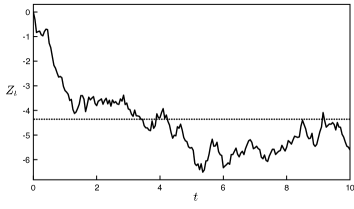
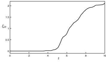
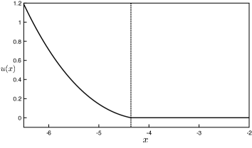
Figure 2: Symmetric regular control equilibrium. The dotted lines indicate the threshold $\theta$.

Remark: The MPE obtained in Theorem 2 exists as long as the solution shown in Lemma 1 exists. Hence, Assumptions 1–3 do not need to hold as long as the single decision maker control problem yields a single-threshold singular control solution.

3 Impact of Stochasticity and Asymmetry

In this section, we examine the implications of stochasticity and asymmetry on the regular control equilibrium that we obtain in Section 2.4. This is an important inquiry because most realistic situations often possess stochastic state variables and heterogeneity among the players. We first examine the case of deterministic $Z$ in Section 3.1 and contrast its equilibrium to that of the stochastic game. We find that the contrast between a single decision maker solution and an equilibrium is starker in the stochastic case. Then we examine an asymmetric game in Section 3.2 and find that a regular control MPE does not exist in an asymmetric game. Instead, asymmetry leads to asymmetric equilibria with singular control strategies.

3.1 Deterministic Game

To examine the impact of stochasticity, we will simply discuss the deterministic case of Example 2 and contrast it to the stochastic case.

Example 3: We revisit the model of Example 2 and set $\sigma=0$ and $x_{c}=-\infty$. Then the characteristic operator

$$\mathcal{A}=\mu\partial_{z}-r$$

is a first-order differential operator, and there is only one fundamental solution $\phi(x)=\exp(rx/\mu)$ that satisfies $\mathcal{A}\phi(x)=0$. Furthermore,

$$(R\pi)(x)=\frac{1}{r}-\frac{\exp(\nu x)}{r-\mu\nu}\>,$$

where we assume $\mu\nu<r$. The critical threshold of control is given by

$$\theta=\frac{1}{\nu}\ln\frac{kr}{|\nu|}\;.$$

As in Example 2, $u(\cdot)$ is given by (2.7). It is straightforward to verify that $\lim_{x\uparrow\theta}u(x)=0$, $\lim_{x\uparrow\theta}u^{\prime}(x)=0$ and that $u^{\prime\prime}(x)>0$ for all $x<\theta$, which implies that $u^{\prime}(x)<0$ for all $x<\theta$. Furthermore, there exists $\eta<\theta$ at which $\mu+2u(\eta)=0$ so that $dZ_{t}/dt<0$ for $Z_{t}>\eta$ and $dZ_{t}/dt>0$ for $Z_{t}<\eta$.

Lastly, we can show that $Z_{t}$ asymptotically approaches $\eta$ if $Z_{0}\neq\eta$. Define $y_{t}=Z_{t}-\eta$. For $y_{t}$ sufficiently close to 0, we have

$$\frac{dy_{t}}{dt} =\mu+2u(y_{t}+\eta)=\mu+2u(\eta)+2u^{\prime}(\eta)y_{t}+O(y_{t}^{2})$$

$$=2u^{\prime}(\eta)y_{t}+O(y_{t}^{2})\>,$$

where we used the fact that $\mu+2u(\eta)=0$ in the last equality. Recall that $u^{\prime}(\eta)<0$; thus, $|y_{t}|=|y_{0}|\exp[2u^{\prime}(\eta)t+O(y_{t})]$ for large $t$, which implies $\lim_{t\rightarrow\infty}y_{t}=0$. Hence, $\eta$ is the steady state of $Z$. Figure 3 illustrates $Z_{t}$ as a function of $t$ in the equilibrium where $\theta=-4.0132$ and $\eta=-5.68646$.

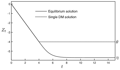
Figure 3: Deterministic solutions.

In the deterministic case of the single decision maker problem, $Z_{t}$ follows the horizontal line $z=\theta$ as soon as $Z_{t}$ hits $\theta$. Thus, $\theta$ is the steady state of the single decision maker solution. Hence, in the deterministic model, the behavior of $Z_{t}$ exhibits very little qualitative difference between the single decision maker solution and the equilibrium of the game. In particular, an outside observer will not be able to tell the difference between the two solutions except that the steady state values differ. The difference in the steady state value of $Z$ can be simply attributed to the free rider effect: the players are less willing to contribute to the common good, so the steady state is lower.

In contrast, in the presence of stochasticity ($\sigma>0$), the behavior of $Z_{t}$ is markedly different as illustrated in Figures 1 and 2: in the single decision maker’s case, $Z_{t}$ is reflected off of the threshold $\theta$, whereas in the equilibrium of the game, $Z_{t}$ can assume any value although it tends to fluctuate around $\theta$. We conclude that stochasticity induces qualitatively different behaviors between the two solutions and hence renders the regular control equilibrium observable to an outsider.

3.2 Asymmetric Game

Next, we examine the impact of asymmetry between the two players. We first show that a regular control MPE is absent in an asymmetric game in Section 3.2.1, and then we construct the simplest class of asymmetric equilibria in Section 3.2.2 and demonstrate that they exhibit the key characteristics of a singular control solution.

3.2.1 Absence of a Regular Control MPE

Suppose that $\theta_{i}\neq\theta_{j}$ because of asymmetry ($k_{i}\neq k_{j}$ and/or $\pi_{i}\neq\pi_{j}$), where $\theta_{i}$ is the unique solution to the equation

$$\frac{k_{i}-(R\pi_{i})^{\prime}(\theta_{i})}{\phi^{\prime}(\theta_{i})}=-\frac{(R\pi_{i})^{\prime\prime}(\theta_{i})}{\phi^{\prime\prime}(\theta_{i})}\>\>.$$

For analytical tractability, we make the following additional assumption:

Assumption 1

$\mu^{\prime}(x)+\pi^{\prime}(x)-rk\neq 0$ almost everywhere $x\in I$.

Assumption 1 ensures that $\mu(x)+\pi(x)-rk$ is never constant within any given non-empty interval. It gives a non-trivial structure to the Hamilton-Jacobi-Bellman (HJB) equation of the payoff function.

The following theorem establishes that there is no payoff function $V_{i}(\cdot;\xi)\in C^{2}(I)$ associated with a regular control MPE.

Theorem 1

If $\theta_{i}\neq\theta_{j}$, then there is no regular control MPE $\xi=(\xi_{i},\xi_{j})\in\Sigma_{i}\times\Sigma_{j}$ such that $V_{i}(\cdot;\xi)\in C^{2}(I)$ for $i=1,2$.

The implication of Theorem 1 is that an MPE of an asymmetric game must involve singular control. Hence, the natural next step is to explore the form of such a singular control MPE in an asymmetric game, which is the goal of Section 3.2.2.

Remark 1: Strictly speaking, Theorem 1 does not necessarily preclude the possibility of an equilibrium with payoffs $V_{i}(\cdot;\xi)$ that do not belong to $C^{2}(I)$ such as a general viscosity solution. In this paper, we limit ourselves to equilibria that produce classic solutions only and defer the possibility of an equilibrium with non-$C^{2}(I)$ viscosity solutions to future endeavors. We also remark that we do not attempt to exclude the possibility of an equilibrium $\xi$ that does not belong to $\Sigma_{i}\times\Sigma_{j}$. This possibility is beyond the scope of the paper because of the issue of the existence of the unique solution to the SDE for $Z_{t}$; this is a common restriction in stochastic control theory (Øksendal and Sulem, 2005).

Remark 2: Even in an asymmetric game, it is possible to have some combinations of $k_{i}$ and $\pi_{i}(\cdot)$ such that $\theta_{1}=\theta_{2}$. In this case, a regular control MPE is possible because Theorem 2 is applicable.

As a corollary, we can also exclude the possibility of an MPE in which there is a common regular control region $(\alpha,\beta)$ for some $\alpha>a$ and a no-control region $[\beta,b)$. (We remark that the proof of Theorem 1 establishes that the regular control regions of the two players must coincide.) We remain agnostic about what happens in the region $(a,\alpha]$, however, except that $(a,\alpha]$ should contain singular control regions $D_{1}$ and $D_{2}$ if they exist. Again, we focus on an MPE with classical solutions, i.e., $V_{i}(\cdot;\xi)\in C^{2}(I\backslash D_{j})$.

Corollary 1

There is no MPE $\xi\in\Sigma_{i}\times\Sigma_{j}$ such that $V_{i}(\cdot;\xi)\in C^{2}(I\backslash D_{j})$ with a common regular control region $(\alpha,\beta)$ for some $\alpha>a$ and a no-control region $[\beta,b)$.

Its proof essentially follows that of Theorem 1, so it is omitted.

3.2.2 Non-regular Control Asymmetric MPE

By virtue of Theorem 1, an asymmetric game allows no regular control MPE, so any MPE must involve some singular control by at least one player. Furthermore, Corollary 1 implies that the only possible equilibria are the ones with a singular control region $[\alpha,\beta]$ of one player and a no-control region $(\beta,b)$. Our goal is to present the simplest class of such equilibria and compare its characteristics to those of the regular control MPE. Although our main focus is on strictly asymmetric games, we will keep our discourse general and implicitly include the case of a symmetric game.

As a candidate for an asymmetric MPE, we consider a strategy profile $\xi$ in which player 1 exerts singular control in the interval $[\theta^{\prime},\theta_{1}]$ and regular control in $(a,\theta^{\prime})$ for some $\theta^{\prime}<\theta_{1}$ while player 2 exerts regular control in $(a,\theta^{\prime})$. Furthermore, we define the regular control rate functions

$$u_{1}(x) =\begin{cases}-\frac{1}{k_{2}}[\mathcal{A}U_{2}(x)+\pi_{2}(x)]&\text{for}\>x<\theta^{\prime}\>,\\ 0&\text{otherwise}\end{cases}\>,$$ (3.1)

$$u_{2}(x) =\begin{cases}-\frac{1}{k_{1}}[\mathcal{A}U_{1}(x)+\pi_{1}(x)]&\text{for}\>x<\theta^{\prime}\>,\\ 0&\text{otherwise}\end{cases}\>,$$ (3.2)

where $U_{1}(\cdot)$, $U_{2}(\cdot)$ are given by

$$U_{1}(x) =V_{1}(x)\;,$$

$$U_{2}(x) =\begin{cases}B\phi(x)+(R\pi_{2})(x)&x\geq\theta_{1}\\ U_{2}(\theta_{1})&x\in(\theta^{\prime},\theta_{1})\\ U_{2}(\theta_{1})+(x-\theta^{\prime})k_{2}&x\leq\theta^{\prime}\end{cases}\>,$$

Here $V_{1}(\cdot)$ denotes the solution to the single decision maker problem given by (2.4) where $k$, $\theta$ and $\pi$ are respectively replaced by $k_{1}$, $\theta_{1}$ and $\pi_{1}$, and

$$B =-\frac{(R\pi_{2})^{\prime}(\theta_{1})}{\phi^{\prime}(\theta_{1})}\;,$$ (3.3)

$$U_{2}(\theta_{1}) =B\phi(\theta_{1})+(R\pi_{2})(\theta_{1})\>.$$

Note that the functions $U_{1}(\cdot)$, $U_{2}(\cdot)$ are actually the payoff functions associated with the proposed strategy profile $\xi$. In the region $(\theta_{1},b)$, both $U_{1}(\cdot)$ and $U_{2}(\cdot)$ assume the form of continuation region without control. In player 1’s singular control region $[\theta^{\prime},\theta_{1}]$, we have $U_{1}^{\prime}(x)=k_{1}$ because player 1 expends the cost of singular control while $U_{2}^{\prime}(x)=0$ because player 2 does not expend any cost in this region. In the common regular control region $(a,\theta^{\prime})$, both players expend cost in such a way that $U_{i}^{\prime}(x)=k_{i}$.

By Theorem 1, to confirm that the strategy profile $\xi$ is an MPE, we only need to verify the following sufficient conditions:

$$U_{2}^{\prime}(x) \leq k_{2}\>\forall x\in I\backslash\{\theta_{1},\theta^{\prime}\},$$ (3.4)

$$\mathcal{A}U_{2}(x)+\pi_{2}(x) \leq 0\;\forall x\in I\backslash\{\theta_{1},\theta^{\prime}\},$$ (3.5)

$$u_{1}(\cdot)\in\mathcal{U}\,,\> u_{2}(\cdot)\in\mathcal{U}\quad.$$ (3.6)

Proposition 1

Suppose that Assumptions 1–3 hold and (3.4)-(3.6) are satisfied. Then the strategy profile $\xi$ is an MPE with the payoff functions given by $V_{1}(x;\xi)=U_{1}(x)$ and $V_{2}(x;\xi)=U_{2}(x)$.

Example 4: Recall Example 2 and set $\mu=-1$, $\sigma=r=k_{1}=k_{2}=1$, $\rho=2$, and $x_{c}=-10$ just as in Figure 2. Then $\theta=-4.3605$ is the boundary of the control region. Here we can construct an asymmetric equilibrium as in Proposition 1 because we can verify that any choice of $\theta^{\prime}<\theta_{1}=\theta$ satisfies conditions (3.4) and (3.5). Hence, there is a continuum of asymmetric equilibria parameterized by $\theta^{\prime}\in(-\infty,\theta_{1})$. Figure 4 illustrates a numerical example of the case $\theta^{\prime}=-6$. Note that even if we set $k_{1}<k_{2}$, the qualitative features of this asymmetric equilibrium continue to hold.

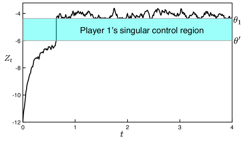
Figure 4: Sample path of $Z_{t}$ in an asymmetric equilibrium.

In particular, Figure 4 illustrates the case when $Z_{0}<\theta^{\prime}$. Before $Z_{t}$ hits $\theta^{\prime}$ for the first time, $Z_{t}$ is subject to regular control of both players. Upon reaching $\theta^{\prime}$, $Z_{t}$ is subject to singular control by player 1 and is boosted up to $\theta_{1}$. Once $Z_{t}$ enters the region $[\theta_{1},\infty)$, the threshold $\theta_{1}$ takes the role of a reflecting boundary for $Z_{t}$ because of player 1’s singular control strategy. If $Z_{t}\in[\theta_{1},\infty)$, the equilibrium reduces to the single decision maker solution.

As illustrated by the example, asymmetric non-regular equilibria exist even for the symmetric game where $k_{1}=k_{2}$ and $\pi_{1}=\pi_{2}$. However, if the two players are identical to each other, the players are likely to be drawn to the symmetric equilibrium. For instance, suppose that the equilibrium shown in Figure 4 is the outcome of the symmetric game. Then eventually player 1 ends up being the only one contributing to the common good every time $Z_{t}$ hits $\theta$, so he will feel that the current equilibrium is unfair to him. Consequently, he will likely attempt to switch to a more equitable equilibrium. Thus, the symmetric regular MPE is the likely focal point equilibrium (Fudenberg and Tirole, 1991). In contrast, in an asymmetric game in which the two players have unequal thresholds $\theta_{i}\neq\theta_{j}$, the only possible equilibrium is an asymmetric non-regular control one by virtue of Theorem 1.

One interesting question regards which player exerts singular control. In the numerical example above, we can fix $k_{1}=1$ and vary the value of $k_{2}$ and see how that affects the equilibrium. It can be numerically verified that the MPE of Proposition 1 exists as long as $k_{2}\geq 0.5383$. If $k_{2}$ is less than the critical value 0.5383, then (3.4) is violated, so the MPE is not possible. Intuitively, if $k_{2}$ is sufficiently low, then player 2 has strong incentive to exert singular control, and knowing this, player 1 would never exert singular control. In this case, the only equilibrium is the one in which player 2 exerts singular control. Thus, sufficiently high asymmetry induces the more efficient player to exert singular control in an equilibrium. If the asymmetry is modest, then either player can be the one who exerts singular control.

In summary, the MPE obtained by Proposition 1 is the simplest form of asymmetric equilibria. In these equilibria, $Z_{t}$ eventually ends up in the region $[\theta_{1},b)$ and subject to the reflecting boundary at $\theta_{1}$. Thus, in the long run, $Z_{t}$ is subject to the singular control policy of player 1 just as in the single decision maker’s case, and it is not plagued by the gradualism of the regular control MPE of Section 2.4. Therefore, we conclude that asymmetry reduces inefficiency.

4 Discussions

4.1 Dimensionality of the State Variable

In contrast to the singular control equilibria obtained in, for example, Ghemawat and Nalebuff (1990), Steg (2012), Battaglini et al. (2014), Ferrari et al. (2017), and Appendix B, a regular control equilibrium arises in our model. We speculate that we obtain a contrasting result because of the difference in the dimensionality of the state variable. In the model that we study, the state variable $Z_{t}$ is one-dimensional; the control variables $\xi_{it}$ and $\xi_{jt}$ only add to $Z_{t}$, so they are not independent state variables that stand alone. In contrast, in the examples from the literature as well as the R&D spillover game analyzed in Appendix B, the state variables are multidimensional because the players’ control variables are decoupled from the state variable. For instance, in the R&D game of Appendix B, the state variable is two-dimensional: $(\lambda_{1t},\lambda_{2t})$, where $\lambda_{it}$ is the current level of R&D effort of firm $i$. Consequently, the possibility of a subgame with $\lambda_{1t}\neq\lambda_{2t}$ is allowed, so the state variable is allowed to be asymmetric between the two players. However, as shown by Section 3.2.2, the regular control equilibrium of Theorem 2 hinges on the symmetry of the state variable between the two players so that they share the common regular control region (see the proof of Theorem 2). Thus, we anticipate that the emergence of a regular control equilibrium is driven by the single-dimensionality of the state variable.

4.2 N-Player Game

We can straightforwardly generalize Theorem 2 to an $N$-player game for $N>2$ by constructing a symmetric regular control equilibrium. We first define $u^{N}(\cdot)$ as follows:

$$u^{N}(x)=\begin{cases}-\frac{1}{k(N-1)}\left(\mathcal{A}V(x)+\pi(x)\right)&\text{for}\;x<\theta\\ 0&\text{for}\;x\geq\theta\end{cases}\>,$$

where $V(\cdot)$ is given by (2.4). Then it can be verified that a strategy profile $\xi$ in which each player $i$ exerts a regular control of $d\xi_{it}=u^{N}(Z_{t})dt$ constitutes a MPE. This is because the HJB equation (condition (iii) of Theorem 1) for each player’s payoff function continues to be satisfied when all $N-1$ opponents exert the regular control of $u^{N}(Z_{t})dt$.

4.3 Relation to Mixed Strategy Equilibrium of War of Attrition

There exists a close analogy between the regular control equilibrium obtained in Theorem 2 and the mixed strategy equilibrium of a war of attrition. In the mixed strategy equilibrium of the canonical war of attrition, each player has control over the hazard rate of exit, which is analogous to the rate of regular control in our model. Similarly, a pure strategy concession (a deterministic concession) in a war of attrition is analogous to the singular control strategy in our model.

The analogy between the two equilibrium solutions goes even further with the impact of asymmetry. In a stochastic extension of a war of attrition game, the mixed strategy MPEs disappear when the players’s reward from concession is asymmetric (Georgiadis et al., 2019). This is analogous to our result that a completely regular control MPE disappears when the players are asymmetric.

5 Conclusions

We examine a stochastic game of variable contribution as a generalization of a war of attrition. In particular, we analyze a stochastic game-theoretic extension of the Nerlove-Arrow model, which possesses a novel MPE characterized by regular control. This finding is in contrast to the singular control equilibria possessed by variable concession games with multidimensional state variables. In the examples of singular control equilibria obtained in the literature, the free rider effect manifests in the value of the threshold of the control region, but the action of concession is immediate and not plagued by delay or gradualism. In contrast, the variable contribution game analyzed in Section 2 possesses a regular control equilibrium in which the free rider effect manifests in the gradualism of the players’ actions.

We find that it is important to understand the effect of stochasticity on the game. The state variable $Z$ exhibits qualitatively different behavior under a regular control MPE from that of a single decision maker solution. However, the difference almost disappears if the state variable is deterministic. We conclude that stochasticity renders the gradual MPE observable to an outsider.

We also examine the impact of asymmetry between the players and find that the regular control MPE is not possible under asymmetry. The implication of this finding is that the problem of inefficiency arising from the gradual regular control MPE is mitigated by asymmetry between the players. From a social planner’s perspective, this result suggests that heterogeneity between agents should be cultivated or encouraged when there is a free rider problem with the agents’ contributions to the common good.

The results and their implications of this paper warrant some related future research endeavors. First, it will be interesting to study multidimensional variable concession problems and see if they have gradual regular control MPE even though we speculate that they do not. Second, it will be fruitful to examine an extension of our model in which the players have private types and asymmetric information regarding the cost of contribution. In this case, there is inherent asymmetry between any two players, so the regular control equilibrium may exist only under very stringent conditions. Lastly, just as Wang (2009) finds empirical evidence of a delay in action in a war of attrition, it might be possible to find empirical evidence of gradualism in a regular control equilibrium for a contribution game with a free rider problem such as in generic advertising or investment in public goods.

Appendix A Mathematical Proofs

Proof of Lemma 1: Because the first and second derivatives of $V(\cdot)$ are continuous at $\theta$, the coefficient $A$ and the threshold $\theta$ must satisfy $k=(R\pi)^{\prime}(\theta)+A\phi^{\prime}(\theta)$ and $0=(R\pi)^{\prime\prime}(\theta)+A\phi^{\prime\prime}(\theta)$. The simultaneous equations are solved if we can find $\theta$ that satisfies

$$\frac{k-(R\pi)^{\prime}(\theta)}{\phi^{\prime}(\theta)}=-\frac{(R\pi)^{\prime\prime}(\theta)}{\phi^{\prime\prime}(\theta)}\>.$$ (A.1)

Below we show that there is a unique value of $\theta$ that satisfies this condition and that the resulting solution $V(\cdot)$ satisfies the optimality conditions for singular stochastic control.

As a first step, we show that the function $F(x):=(k-(R\pi)^{\prime}(x))/\phi^{\prime}(x)$ achieves a unique global maximum at $x=\theta\in I$. If this holds, then it is straightforward to verify that (A.1) is satisfied. Note that $(Rq)^{\prime}(x)=(R\pi)^{\prime}(x)-k$ from the definition of $q$ in (2.3) without the player index $i$, so $F(x)=-(Rq)^{\prime}(x)/\phi^{\prime}(x)$. From the theory of diffusive processes (Borodin and Salminen, 1996; Alvarez and Lempa, 2008), it is well-known that

$$(Rq)(x)=B^{-1}\left[\phi(x)\int_{a}^{x}\psi(y)q(y)m^{\prime}(y)dt+\psi(x)\int_{x}^{b}\phi(y)q(y)m^{\prime}(y)dt\right]\>,$$

where

$$B =\frac{1}{S^{\prime}(x)}[\psi^{\prime}(x)\phi(x)-\phi^{\prime}(x)\psi(x)]\;,$$

$$m^{\prime}(x) =\frac{2}{\sigma^{2}(x)S^{\prime}(x)}\quad,$$

$$S^{\prime}(x) =\exp\left(-\int_{0}^{x}\frac{2\mu(y)}{\sigma^{2}(y)}dy\right)\;.$$

Thus, we have

$$\frac{dF(x)}{dx} =-\frac{2S^{\prime}(x)}{\sigma^{2}(x)[\phi^{\prime}(x)]^{2}}L(x)\>,$$ (A.2)

$$\text{where}\;L(x) =-\frac{q(x)\phi^{\prime}(x)}{S^{\prime}(x)}-r\int_{x}^{b}\phi(y)q(y)m^{\prime}(y)dy\>.-x$$ (A.3)

By the definitions of $m^{\prime}(\cdot)$ and $S^{\prime}(\cdot)$, we can derive the equality $d(\phi^{\prime}(x)/S^{\prime}(x))/dx=r\phi(x)m^{\prime}(x)$ by some algebra, from which we obtain

$$\frac{dL(x)}{dx}=-q^{\prime}(x)\frac{\phi^{\prime}(x)}{S^{\prime}(x)}\>.$$

By Assumption 3 (ii), $q^{\prime}(x)>0$ for $x\in(a,x^{*})$ and $q^{\prime}(x)<0$ for $(x^{*},b)$, we have $dL(x)/dx>0$ for $x\in(a,x^{*})$ and $dL(x)/dx<0$ for $x\in(x^{*},b)$. From $\lim_{x\rightarrow a}\phi^{\prime}(x)/S^{\prime}(x)=-\infty$ (p. 19 of Borodin and Salminen (1996)) and $\lim_{x\rightarrow a}q(x)=-\infty$ from Assumption 3 (iii), we have for $y$ sufficiently close to $a$,

$$L(y)-\lim_{x\rightarrow a}L(x)=\lim_{x\rightarrow a}\int_{x}^{y}\frac{dL(u)}{du}du=\lim_{x\rightarrow a}\int_{x}^{y}[-q^{\prime}(u)]\frac{\phi^{\prime}(u)}{S^{\prime}(u)}du>\frac{\phi^{\prime}(y)}{S^{\prime}(y)}\lim_{x\rightarrow a}\int_{x}^{y}[-q^{\prime}(u)]du=\infty\>,$$

so that $\lim_{x\rightarrow a}L(x)=-\infty$. Furthermore, because $\lim_{x\rightarrow b}q(x)\phi^{\prime}(x)/S^{\prime}(x)=0$ from Assumption 3 (iii), we also have $\lim_{x\rightarrow b}L(x)=0$ by the expression (A.3). From the continuity of $L(\cdot)$ and the sign change of $dL(x)/dx$, it follows that $L(\theta)=0$ for some unique point $\theta\in(a,x^{*})$. Since $L(\cdot)$ is monotonically increasing in the interval $(a,x^{*})$, $L(\cdot)$ turns from negative to positive at $\theta$. Combined with the behavior of $L(x)$ in the limits $x\rightarrow a,b$, we conclude that $L(x)$ is negative in the interval $(a,\theta)$ and positive in the interval $(\theta,b)$. From (A.2), we also conclude that $F(x)$ attains its global maximum at this unique point $\theta$. Thus, (A.1) is also satisfied, which makes $V(\cdot)\in C^{2}(I)$ if $A=F(\theta)$.

The next step is to prove that $V(\cdot)$ satisfies the sufficient conditions (i) and (ii) of the optimality.

(i) First, we show that $\mathcal{A}V(x)+\pi(x)\leq 0$ and $V^{\prime}(x)-k\leq 0$ for all $x\in I$. For $x>\theta$, the form of $V(\cdot)$ guarantees the condition $\mathcal{A}V(x)+\pi(x)=0$. Furthermore, because $F(x)<F(\theta)=A$ for all $x>\theta$, we have $(k-(R\pi)^{\prime}(x))/\phi^{\prime}(x)<A$, from which we obtain

$$V^{\prime}(x)=A\phi^{\prime}(x)+(R\pi)^{\prime}(x)<k$$

for all $x>\theta$.

For $x<\theta$, we have $V^{\prime}(x)=k$ by the form of $V(\cdot)$. Also note that $V^{\prime\prime}(\theta)=0$, $V^{\prime}(\theta)=k$ and $\mathcal{A}V(x)+\pi(x)=0$ for $x>\theta$ so that

$$\lim_{x\downarrow\theta}\mathcal{A}V(x)+\pi(x)=\mu(\theta)k-rV(\theta)+\pi(\theta)=0\>.$$

For any $x<\theta$, we have

$$\mathcal{A}V(x)+\pi(x)-[\lim_{y\downarrow\theta}\mathcal{A}V(y)+\pi(y)] =\mu(x)k-rV(x)+\pi(x)-[\mu(\theta)k-rV(\theta)+\pi(\theta)]$$

$$=q(x)-q(\theta)<0$$

where the inequality is from the fact that $q(\cdot)$ increases in the interval $(a,\theta)$. Thus, $\mathcal{A}V(x)+\pi(x)<0$ for $x<\theta$.

(ii) We just showed that $\mathcal{A}V(x)+\pi(x)=0$ for $x\geq\theta$ and $V^{\prime}(x)-k=0$ for $x\leq\theta$.  

Proof of Theorem 1: To prove the theorem, it is sufficient to show that $U(x)=V_{i}(x;\xi_{i}^{*},\xi_{j})\geq V_{i}(x;\xi_{i},\xi_{j})$ for any arbitrary strategy $\xi_{i}$ of player $i$ that satisfies $d\xi_{it}=u_{i}(t,Z_{t})+d\xi_{it}^{c}+\Delta\xi_{it}$. First, it is straightforward to verify that if $\xi_{i}^{*}$ is the best response, player $i$ should not expend any cost to control $Z$ within $D_{j}$ because player $j$ is already doing so in that region. Thus, one necessary condition for the payoff function of the best response is $U^{\prime}(x)=0$ in the interior of $D_{j}$.

We consider an arbitrary strategy $\xi_{i}$ of player $i$ that satisfies $d\xi_{it}=u_{i}(t,Z_{t})dt+d\xi_{it}^{c}+\Delta\xi_{it}$ for some arbitrary $u_{i}(\cdot)\in\mathcal{U}$. Let $Z$ be the state process dictated by the given strategy profile $(\xi_{i},\xi_{j})$.

By conditions (i) and (iii), $U^{\prime}(\cdot)$ is a bounded function. Furthermore, due to Assumption 1 (i), $e^{-rs}\sigma(Z_{s})\tilde{U}^{\prime}(Z_{s})$ is locally bounded. Hence, the process $M_{t}:=\int_{0}^{t}e^{-rs}\sigma(Z_{s})\tilde{U}^{\prime}(Z_{s})dW_{s}$ is a continuous local martingale. By the definition of a continuous local martingale (Karatzas and Shreve, 1998), there exists a non-decreasing sequence $\{\tau_{n}\}_{n=1}^{\infty}$ of stopping times of $\{\mathcal{F}_{t}\}_{t>0}$ such that $\lim_{n\rightarrow\infty}\tau_{n}=\infty$ a.s. and $\{M_{\tau_{n}\wedge t}:t\in[0,\infty)\}$ is a martingale for each $n$. We first consider any $x\in C_{j}$ as the initial point of $Z$. By the generalized Itô’s formula, we have

$$e^{-r\tau_{n}\wedge t}\tilde{U}(Z_{\tau_{n}\wedge t})= \tilde{U}(x)+\int_{0}^{\tau_{n}\wedge t}e^{-rs}\mathcal{A}\tilde{U}(Z_{s})ds$$

$$+\int_{0}^{\tau_{n}\wedge t}e^{-rs}\tilde{U}^{\prime}(Z_{s})[u_{i}(t,Z_{s})ds+u_{j}(Z_{s})ds+\sum_{l=1}^{2}d\xi_{ls}^{c}]$$

$$+\sum_{0\leq s\leq\tau_{n}\wedge t}e^{-rs}[\tilde{U}(Z_{s})-\tilde{U}(Z_{s^{-}})]+M_{\tau_{n}\wedge t}\>.$$

Taking the expectation of both sides and rearranging terms, we obtain

$$\tilde{U}(x)= \mathbb{E}^{x}[e^{-r\tau_{n}\wedge t}\tilde{U}(Z_{\tau_{n}\wedge t})]-\mathbb{E}^{x}\left[\int_{0}^{\tau_{n}\wedge t}e^{-rs}(\mathcal{A}\tilde{U}(Z_{s})+\tilde{U}^{\prime}(Z_{s})u_{j}(Z_{s})+\tilde{U}^{\prime}(Z_{s})u_{i}(s,Z_{s}))ds\right]$$

$$-\mathbb{E}^{x}\left[\int_{0}^{\tau_{n}\wedge t}e^{-rs}\tilde{U}^{\prime}(Z_{s})\sum_{l=1}^{2}d\xi_{ls}^{c}+\sum_{0\leq s\leq\tau_{n}\wedge t}e^{-rs}[\tilde{U}(Z_{s})-\tilde{U}(Z_{s^{-}})]\right]\>.$$ (A.4)

Here we use the fact that $\mathbb{E}^{x}[M_{\tau_{n}\wedge t}]=0$ because $M_{\tau_{n}\wedge t}$ is a martingale.

Next, we re-express (A.4) as an inequality involving $U(\cdot)$ and $\xi_{i}$ alone. Recall that $\tilde{U}(x)=U(x)$ whenever $x\in C_{j}$, so $\tilde{U}(Z_{t})=U(Z_{t})$ whenever $Z_{t}$ is continuous in time. Thus, if $Z_{s}\in C_{j}$,

$$\mathcal{A}\tilde{U}(Z_{s})+\tilde{U}^{\prime}(Z_{s})(u_{i}(t,Z_{s})+u_{j}(Z_{s}))=\mathcal{A}U(Z_{s})+U^{\prime}(Z_{s})(u_{i}(t,Z_{s})+u_{j}(Z_{s}))\,.$$

We also note that $\tilde{U}^{\prime}(Z_{s})d\xi_{js}^{c}=0$ for all $s$ from condition (i) since $d\xi_{js}^{c}=0$ if $Z_{s}\in D_{j}$ and $\tilde{U}^{\prime}(Z_{s})=U^{\prime}(Z_{s})$ if $Z_{s}\in C_{j}$. Also note that the process $Z_{t}$ spends zero time within $D_{j}$, so $\tilde{U}(Z_{s})-\tilde{U}(Z_{s^{-}})=U(Z_{s})-U(Z_{s^{-}})$ for all $s>0$. Then we can re-express (A.4) as the following equality:

$$U(x)= \mathbb{E}^{x}[e^{-r\tau_{n}\wedge t}U(Z_{\tau_{n}\wedge t})]-\mathbb{E}^{x}\left[\int_{0}^{\tau_{n}\wedge t}e^{-rs}(\mathcal{A}U(Z_{s})+U^{\prime}(Z_{s})u_{j}(Z_{s})+U^{\prime}(Z_{s})u_{i}(s,Z_{s}))ds\right]$$

$$-\mathbb{E}^{x}\left[\int_{0}^{\tau_{n}\wedge t}e^{-rs}U^{\prime}(Z_{s})\sum_{l=1}^{2}d\xi_{ls}^{c}+\sum_{0\leq s\leq\tau_{n}\wedge t}e^{-rs}[U(Z_{s})-U(Z_{s^{-}})]\right]\>.$$ (A.5)

We note that

$$\mathcal{A}U(Z_{s})+U^{\prime}(Z_{s})(u_{i}(t,Z_{s})+u_{j}(Z_{s}))\leq k_{i}u_{i}(t,Z_{s})-\pi_{i}(Z_{s})$$

because of condition (iii). Regarding player $j$’s singular control, we have $U(Z_{s^{-}}+\Delta\xi_{js})-U(Z_{s^{-}})=0$ for any $\Delta\xi_{js}>0$ because of condition (i) that $U^{\prime}(x)=0$ for all $x$ within the interior of $D_{j}$. Lastly, we note that $U^{\prime}(Z_{s})\sum_{l=1}^{2}d\xi_{ls}^{c}\leq k_{i}d\xi_{is}^{c}$ because $U^{\prime}(x)\leq k_{i}$ from condition (iii) and $U^{\prime}(Z_{s})d\xi_{js}^{c}=0$ from condition (i), and $U(Z_{s^{-}}+\Delta\xi_{is})-U(Z_{s^{-}})\leq k_{i}\Delta\xi_{is}$ from $U^{\prime}(x)\leq k_{i}$. Combining all these facts, we obtain

$$U(x)\geq \mathbb{E}^{x}[e^{-r\tau_{n}\wedge t}U(Z_{\tau_{n}\wedge t})]+\mathbb{E}^{x}[\int_{0}^{\tau_{n}\wedge t}e^{-rs}(\pi_{i}(Z_{s})-k_{i}u_{i}(t,Z_{s}))ds]$$

$$-k_{i}\mathbb{E}^{x}[\int_{0}^{\tau_{n}\wedge t}e^{-rs}d\xi_{is}^{c}+\sum_{0\leq s\leq\tau_{n}\wedge t}e^{-rs}\Delta\xi_{is}]\;.$$

Since $U(\cdot)$ is non-decreasing and $U^{\prime}(x)\leq k_{i}$, we have $(U(Z_{t}))^{-}\leq k_{i}(Z_{t})^{-}+C_{0}$ for some $C_{0}>0$. Furthermore, in comparison to the uncontrolled process $X_{t}$, we have $Z_{t}\geq X_{t}$ for any control strategies taken by the players because the controls $\xi_{i}$ and $\xi_{j}$ always boost $Z_{t}$. It follows that $(Z_{t})^{-}\leq(X_{t})^{-}$ for all $t\geq 0$ if $X_{0}=Z_{0}$. By virtue of Assumption 1 (ii), $\{e^{-r\tau}(U(Z_{\tau}))^{-}:\tau>0\;\text{stopping time}\}$ is uniformly integrable under any control strategy profile $(\xi_{i},\xi_{j})$. Thus, we have

$$\liminf_{n\rightarrow\infty}\mathbb{E}^{x}[e^{-r\tau_{n}\wedge t}U(Z_{\tau_{n}\wedge t})]=\mathbb{E}^{x}[\liminf_{n\rightarrow\infty}e^{-r\tau_{n}\wedge t}U(Z_{\tau_{n}\wedge t})]=E^{x}[e^{-rt}U(Z_{t})]\>.$$

From Fatou’s lemma, we have

$$U(x)\geq \liminf_{n\rightarrow\infty}\mathbb{E}^{x}[e^{-r\tau_{n}\wedge t}U(Z_{\tau_{n}\wedge t})]+\liminf_{n\rightarrow\infty}\mathbb{E}^{x}\left[\int_{0}^{\tau_{n}\wedge t}e^{-rs}(\pi_{i}(Z_{s})-k_{i}u_{i}(t,Z_{s}))ds\right]$$

$$-k_{i}\liminf_{n\rightarrow\infty}\mathbb{E}^{x}[\int_{0}^{\tau_{n}\wedge t}e^{-rs}d\xi_{is}^{c}+\sum_{0\leq s\leq\tau_{n}\wedge t}e^{-rs}\Delta\xi_{is}]$$

$$\geq E^{x}[e^{-rt}U(Z_{t})]+\mathbb{E}^{x}[\int_{0}^{t}e^{-rs}(\pi_{i}(Z_{s})-k_{i}u_{i}(t,Z_{s}))ds]$$

$$-k_{i}\mathbb{E}^{x}[\int_{0}^{t}e^{-rs}d\xi_{is}^{c}+\sum_{0\leq s\leq t}e^{-rs}\Delta\xi_{is}]\;.$$

We note that $U(Z_{t})\leq M$ for some $M>0$ because it is bounded from above. Furthermore, because $U^{\prime}(\cdot)$ is bounded from above by $k_{i}$ by condition (iii), we have $(U(Z_{t}))^{-}\leq k_{i}(Z_{t})^{-}+C_{0}$ for some constant $C_{0}>0$. Recall that $(Z_{t})^{-}\leq(X_{t})^{-}$ for the uncontrolled process $X_{t}$ and that $\lim_{t\rightarrow\infty}\mathbb{E}^{x}[e^{-rt}(X_{t})^{-}]=0$ by Assumption 1. Therefore, $\lim_{t\rightarrow\infty}E^{x}[e^{-rt}U(Z_{t})]=0$ is also satisfied, and so we obtain

$$U(x) \geq\mathbb{E}^{x}[\int_{0}^{\infty}e^{-rs}(\pi_{i}(Z_{s})-k_{i}u_{i}(t,Z_{s}))ds]-k_{i}\int_{0}^{\infty}e^{-rs}d\xi_{is}^{c}-k_{i}\sum_{0\leq s<\infty}e^{-rs}\Delta\xi_{is}]$$

$$=V_{i}(x;\xi_{i},\xi_{j})\quad.$$

Since $\xi_{i}$ is an arbitrary strategy of player $i$ that satisfies $d\xi_{it}=u_{i}(t,Z_{t})+d\xi_{it}^{c}+\Delta\xi_{it}$, we have proved that $U(x)$ dominates all payoff functions that belong to the set $\{V_{i}(x;\xi_{i},\xi_{j}):\xi_{i}\in\Sigma_{i}\}$.

Lastly, we consider $Z$ subject to the strategy profile $(\xi_{i}^{*},\xi_{j})$. Note that $\{e^{-r\tau}U(Z_{\tau}):\tau>0\;\text{stopping time}\}$ is uniformly integrable because $U(\cdot)$ is bounded from above and $\{e^{-r\tau}(U(Z_{\tau}))^{-}:\tau>0\;\text{stopping time}\}$ is uniformly integrable. By condition (iv), it is straightforward to verify that all the weak inequalities above can be exactly replaced by equalities if $\xi_{i}$ above is replaced by $\xi_{i}^{*}$. Therefore, $\xi_{i}^{*}$ is the best response among $\Sigma_{i}$ against $\xi_{j}$, and $U(\cdot)$ is the best payoff function of player $i$ within the set $\{V_{i}(x;\xi_{i},\xi_{j}):\xi_{i}\in\Sigma_{i}\}$.  

Proof of Theorem 2: As a first step, we verify that $V(x)$ in (2.4) and $\xi$ given by the proposition satisfy the conditions (i)–(iv) of Theorem 1.

(i) Note that $C_{i}=C_{j}=I$, and $V(\cdot)\in C^{2}(I)$ and that $V(\cdot)$ is non-decreasing. Thus, condition (i) is satisfied. Condition (ii) is not applicable because $D_{1}=D_{2}=\emptyset$.

(iii) and (iv) For $x>\theta$, we have $V^{\prime}(x)\leq k$ by the definition of $V(\cdot)$, and $\mathcal{A}V(x)+\pi(x)=0$, so condition (iii) is satisfied. For $x\leq\theta$, we have $V^{\prime}(x)=k$ and

$$\mathcal{A}V(x)+\pi(x)+u(x)V^{\prime}(x)+v(U^{\prime}(x)-k)=0$$

for any arbitrary $v$ by the definition of $u(\cdot)$. Thus, condition (iii) is also satisfied for $x\leq\theta$. Because $D_{1}=D_{2}=\emptyset$, it also follows that condition (iv) is satisfied.

Thus, we have proved that $\xi=(\xi_{i},\xi_{j})$ is a strategy profile that belongs to $\Sigma=\Sigma_{i}\times\Sigma_{j}$ and that $V_{i}(x;\xi)=\sup_{\zeta_{i}\in\Sigma_{i}}V_{i}(x;\zeta_{i},\xi_{j})=V(x)$ for both $i=1,2$. This does not necessarily mean that $\xi$ is a Nash equilibrium. More precisely, we need to prove that $\xi_{i}$ is the best response among $\Xi_{i}$. To prove it, we only need to show that $V(x)=\sup_{\zeta_{i}\in\Xi_{i}}V_{i}(x;\zeta_{i},\xi_{j})$, i.e., that $V(\cdot)$ is player $i$’s optimal value function given $\xi_{j}$. We do so by showing that there exists a singular control strategy $\xi_{i}^{*}\in\Xi_{i}$ such that $V(x)=V_{i}(x;\xi_{i}^{*},\xi_{j})$ and that $V(\cdot)$ satisfies the optimality conditions for player $i$ given in Section 2.2.

Given $\xi_{j}$, the SDE of $Z$ and its $r$-excessive characteristic operator are given by

$$dZ_{t} =[\mu(Z_{t})+u_{j}(Z_{t})]dt+\sigma(Z_{t})dW_{t}\>,$$

$$\mathcal{A}_{\xi_{j}} =\frac{1}{2}\sigma(x)^{2}\partial_{x}^{2}+[\mu(x)+u_{j}(x)]\partial_{x}-r\>.$$

Consider $\xi_{i}^{*}$ with a singular control region $D_{i}=(a,\theta]$, which is consistent with the fact that $V^{\prime}(x)=k$ for all $x\in D_{i}$. First, note that $\mathcal{A}_{\xi_{j}}V(x)+\pi(x)=0$ and $V^{\prime}(x)\leq k$ for all $x\in I$. Second, it follows that $[\mathcal{A}_{\xi_{j}}V(x)+\pi(x)][V^{\prime}(x)-k]=0$ for all $x\in I$. Thus, all the conditions of the optimality are satisfied, and we conclude that $V(x)=\sup_{\zeta_{i}\in\Xi_{i}}V_{i}(x;\zeta_{i},\xi_{j})$.  

Proof of Theorem 1: Assume that there exists a regular control MPE with a payoff function $V_{i}(\cdot;\xi)\in C^{2}(I)$. To prove Theorem 1, we establish the following two statements: (i) The control regions of both players must coincide. (ii) Player $i$’s control region must be $(a,\theta_{i})$. Given (i) and (ii), because of the assumption $\theta_{i}\neq\theta_{j}$, we arrive at a contradiction and hence prove the theorem.

Below we employ Theorem 11.2.1 of Øksendal (2003) to prove (i) and (ii). For the theorem to be applicable, a few conditions have to be satisfied. First, $V_{i}(\cdot;\xi)\in C^{2}(I)$ has to be satisfied, which is assume above. Second, we need to have $|\mathcal{A}V_{i}(x;\xi)|<\infty$ $\forall x\in I$, which is satisfied because of Assumption 1. Lastly, we need to have $|[u_{i}(x)+u_{j}(x)]V_{i}^{\prime}(x;\xi)|<\infty$ $\forall x\in I$, which is satisfied because we limit $\xi$ to $\Sigma_{i}\times\Sigma_{j}$. Thus, Theorem 11.2.1 of Øksendal (2003) is applicable.

(i) We first prove that the regular control regions $E_{i}=\{x\in I:u_{i}(x)>0\}$ of both players must coincide, i.e., $E_{1}=E_{2}$. Suppose that there exists a non-empty open set $F_{i}\subset E_{i}\backslash E_{j}$ such that $u_{i}(x)>0$ but $u_{j}(x)=0$ whenever $x\in F_{i}$. Note that $V_{i}^{\prime}(x;\xi)\leq k_{i}$; if there exists an interval in which $V_{i}^{\prime}(x;\xi)>k_{i}$, then it behooves player $i$ to adopt a singular control strategy in this interval, which contradicts the assumption that the equilibrium is characterized only by regular control strategies. By Theorem 11.2.1 of Øksendal (2003), $V_{i}(x;\xi)$ must satisfy the following HJB equation in $F_{i}$:

$$\mathcal{A}V_{i}(x;\xi)+\pi_{i}(x)+u_{i}(x)[V_{i}^{\prime}(x;\xi)-k_{i}]=0$$

such that $u_{i}(x)>0$ only if $V_{i}^{\prime}(x;\xi)=k_{i}$. Here we used the fact that $u_{j}(x)=0$ in $F_{i}$. By the assumption that $u_{i}(x)>0$ for all $x\in F_{i}$, $V_{i}(x;\xi)=v_{0}+k_{i}x$ for some constant $v_{0}$. Then the solution to

$$\mathcal{A}V_{i}(x;\xi)+\pi_{i}(x)=\mu(x)k_{i}-r[v_{0}+k_{i}x]+\pi_{i}(x)=0$$

cannot be a non-empty open interval according to Assumption 1. Thus, the necessary HJB condition cannot be satisfied in $F_{i}$. It follows that a non-empty open set $F_{i}\subset E_{i}\backslash E_{j}$ cannot exist for either $i$. Because $u_{i}(\cdot)$ is Lipschitz continuous, it implies $E_{i}=E_{j}$. For convenience, we let $E=E_{i}=E_{j}$ denote the common regular control region for the remainder of this proof.

(ii) By Theorem 11.2.1 of Øksendal (2003), $V_{i}(\cdot;\xi)$ must satisfy

$$\mathcal{A}V_{i}(z;\xi)+\pi_{i}(z)+u_{j}(z)\partial_{z}V_{i}(z;\xi)+u_{i}(z)[\partial_{z}V_{i}(z;\xi)-k_{i}]=0\>,$$ (A.6)

where $u_{i}(x)>0$, $V_{i}^{\prime}(x;\xi)=k_{i}$ and $u_{j}(x)>0$ must be satisfied only if $x\in E$, and $u_{i}(x)=u_{j}(x)=0$ and $V_{i}^{\prime}(x;\xi)<k_{i}$ must be satisfied for $x\not\in E$. Furthermore, since $u_{j}(x)>0$ for $x\in E$, in order for (A.6) to hold, $\mathcal{A}V_{i}(x;\xi)+\pi_{i}(x)<0$ needs to be satisfied for $x\in E$. In summary, the most salient necessary conditions are $[\mathcal{A}V_{i}(x;\xi)+\pi_{i}(x)][V_{i}^{\prime}(x;\xi)-k_{i}]=0$, $\mathcal{A}V_{i}(x;\xi)+\pi_{i}(x)\leq 0$, and $V_{i}^{\prime}(x;\xi)\leq k_{i}$. These conditions exactly coincide with the optimality conditions for a single decision maker singular stochastic control problem given in Section 2.2. By virtue of Lemma 1, there is a unique function $V_{i}^{*}(\cdot)$ given by (2.4) where $\theta$ and $\pi$ are replaced by $\theta_{1}$ and $\pi_{1}$ that satisfies these necessary conditions. Based on the form of $V_{i}^{*}(\cdot)$ given by (2.4), the regular control region is $E_{i}=(a,\theta_{i})$.

From (ii), we conclude that the equilibrium is characterized by the player’s control region $E_{i}=(a,\theta_{i})$ and $E_{j}=(a,\theta_{j})$. However, as established by (i), the two control regions must coincide ($E_{i}=E_{j}$), which is not possible if $\theta_{i}\neq\theta_{j}$. Therefore, there is no regular control strategy equilibrium with associated payoff functions $V_{i}(\cdot;\xi)\in C^{2}(I)$.  

Proof of Proposition 1: Note that $\xi_{1}$ continuously evolves in $C_{1}=(a,\theta^{\prime})\cup(\theta,b)$ and $\xi_{2}$ continuously evolves in $C_{2}=I$ according to the strategy profile $\xi$. To prove the proposition, it is sufficient to verify that $U_{1}(\cdot)$ and $U_{2}(\cdot)$ with the strategy profile $\xi$ satisfy all the conditions of Theorem 1. The complete proof exactly parallels that of Theorem 2.

We first assume $\xi_{2}$ and examine $U_{1}(\cdot)$. First, it is straightforward to verify that $U_{1}(\cdot)$ satisfies conditions (i) and (ii) of Theorem 1 because $C_{2}=I$. Hence, we only need to verify (iii) and (iv). Because of the forms of $u_{1}(\cdot)$ and $u_{2}(\cdot)$ given in (3.1) and (3.2), we have $\mathcal{A}U_{1}(x)+\pi_{1}(x)+u_{2}(x)U_{1}^{\prime}(x)=0$ for all $x<\theta^{\prime}$. We also have $U_{1}^{\prime}(x)\leq k_{1}$ for all and $x\in I$, and, in particular, $U_{1}^{\prime}(x)=k_{1}$ for all $x<\theta_{1}$. Hence, conditions (iii) and (iv) are satisfied.

Next, we verify that $U_{2}(\cdot)$ given $\xi_{1}$ satisfies the conditions (i)-(iv) of Theorem 1.

(i) Note that $D_{1}=[\theta^{\prime},\theta_{1}]$ and that $U_{2}(\cdot)$ is constant in $D_{1}$. Furthermore, by the definition of $B$ in (3.3), we have $\lim_{x\downarrow\theta_{1}}U_{2}^{\prime}(x)=0$. Note that, by the nature of a singular control, $\xi_{1t}^{l}$ evolves only at the right-most boundary of the singular control region $D_{1}$. This implies that $U_{2}^{\prime}(Z_{t})=0$ whenever $d\xi_{1t}^{l}>0$ so that $U_{2}^{\prime}(Z_{t})d\xi_{1t}^{l}=0$. Hence, (i) is satisfied.

(ii) The first derivative of $U_{2}(\cdot)$ is discontinuous (not defined) at $x=\theta^{\prime}$, and its second derivative is in general not defined at $x=\theta_{1}$. However, given the first and second derivatives of $U_{2}(\cdot)$ near $\theta^{\prime}$ and $\theta_{1}$, it is always possible to construct a function $\tilde{U}_{2}(\cdot)\in C^{2}(I)$ such that $\tilde{U}_{2}(x)=U(x)$ for all $x\in C_{1}=(a,\theta^{\prime})\cup(\theta_{1},b)$ as long as $\theta^{\prime}<\theta_{1}$.

(iii) For $x>\theta_{1}$, we have $\mathcal{A}U_{2}(x)+\pi_{2}(x)=0$ by the form of $U_{2}(\cdot)$, and $U_{2}^{\prime}(x)\leq k_{2}$ is satisfied so that $v_{2}[U_{2}^{\prime}(x)-k_{2}]\leq 0$ for any $v_{2}\geq 0$. Hence, condition (iii) is satisfied for $(\theta_{1},b)$. For all $x<\theta^{\prime}$, we have $\mathcal{A}U_{2}(x)+\pi_{2}(x)+u_{1}(x)k_{2}=0$ by the form of $u_{1}(\cdot)$, and $U_{2}^{\prime}(x)=k_{2}$. Thus, condition (iii) is satisfied for all $x\in C_{1}$. Furthermore, it is straightforward to verify (iv) from the forms of $u_{i}(\cdot)$.  

Appendix B R&D Game with Spillover

An example of variable contribution games is an R&D game with spillover, which often occurs in high-tech industries. The technological advances made by one firm most often spill over to another firm through various means such as reverse engineering, leakage of information due to geographic proximity, etc.

We consider two firms engaging in R&D to develop a new technology. For simplicity, we assume that the outcome of one firm’s successful completion of R&D completely spills over to the other. We also assume that the two firms are not in direct competition with each other because they are in two separate markets although they use the same technology. This model is an extension of an attrition game: each firm would rather that its opponent conducts the R&D. Thus, the R&D effort is subject to a free rider problem. Unlike the canonical attrition game, the two firms’ levels of R&D effort are the state variables.

Let $R$ denote the reward to each firm from the new technology, irrespective of which firm develops it, and let $\lambda_{it}\geq 0$ denote the effort level of firm $i\in\{1,2\}$ at time $t$. The completion time of firm $i$’s R&D is an exponential random variable with the instantaneous arrival rate of $\lambda_{it}$. Hence, by the property of a Poisson process, the instantaneous arrival rate of the first completion of R&D is given by $\lambda_{1t}+\lambda_{2t}$. We model the cost of maintaining the effort level of $\lambda_{it}$ as $c\lambda_{it}^{2}/2$ per unit time. Furthermore, in order to increase the effort level by $\Delta\lambda_{it}>0$, firm $i$ has to spend $k\Delta\lambda_{it}$ for some $k>0$. Each firm $i$ can increase $\lambda_{it}$ by any amount at any time but can never decrease it.

Let $(\lambda_{it})_{t\geq 0}$ denote the non-decreasing process of the effort level of firm $i$, and let $\hat{T}_{i}$ denote the random completion time of firm $i$’s R&D given the process $(\lambda_{it})_{t\geq 0}$. Given the strategy profile $\Lambda=((\lambda_{it})_{t\geq 0},(\lambda_{jt})_{t\geq 0})$, firm $i$’s payoff at $t=0$ is given by

$$V_{i}(\Lambda)=\mathbb{E}\left[\int_{0}^{\hat{T}_{1}\wedge\hat{T}_{2}}e^{-rt}(-\frac{c}{2}\lambda_{it}^{2})dt+e^{-r\hat{T}_{1}\wedge\hat{T}_{2}}R-\int_{0}^{\hat{T}_{1}\wedge\hat{T}_{2}}e^{-rt}kd\lambda_{it}\right]\>.$$ (B.1)

The goal of this section is to demonstrate the existence of a subgame perfect equilibrium characterized by singular control strategies. Hence, we focus on a symmetric equilibrium in which the firms immediately boost $\lambda_{it}$ to the equilibrium level. In particular, we show that there exists a symmetric subgame perfect equilibrium in which both firms immediately set their effort level at a unique value $\lambda^{*}$ given by

$$\lambda^{*}=\frac{r}{8k+3c}\left[-(4k+c)r+\sqrt{(4k+c)^{2}+2(R/r-k)(8k+3c)}\right]\>,$$ (B.2)

and maintain it until the end of the game. We can verify that this is an equilibrium by the first-order optimality condition for each player’s best response. Here we assume that the reward is sufficiently large so that

$$(4k+c)^{2}+2(R/r-k)(8k+3c)>0\>.$$

Proposition 1

Suppose that the initial effort levels are given by $\lambda_{i0}<\lambda^{*}$ and $\lambda_{j0}<\lambda^{*}$. Then there exists a subgame perfect equilibrium in which both firms boost their effort levels up to $\lambda^{*}$ at time zero.

Proof: Suppose that firm 2’s strategy is to boost the effort level to a level $\lambda_{2}$ at time zero and keep it at this level until the end of the game. Our goal is to obtain the best response of firm 1. Let $\lambda_{1,0}$ denote the initial effort level of firm 1. Given firm 2’s strategy, firm 1’s best response should be to similarly boost the effort level to some value $\lambda$ and keep it until the end of the game because of the Markov property of the Poisson process.

As a first step, we compute the following:

$$\mathbb{E}[\exp(-r\hat{T}_{1}\wedge\hat{T}_{2})]= \int_{0}^{\infty}\lambda_{2}e^{-\lambda_{2}t_{2}}dt_{2}\int_{0}^{t_{2}}\lambda e^{-\lambda t_{1}}dt_{1}e^{-rt_{1}}$$

$$+\int_{0}^{\infty}\lambda e^{-\lambda t_{1}}dt_{1}\int_{0}^{t_{1}}\lambda_{2}e^{-\lambda_{2}t_{2}}dt_{2}e^{-rt_{2}}$$

$$= \frac{\lambda+\lambda_{2}}{r+\lambda+\lambda_{2}}\>.$$

From () we obtain

$$V_{1}(\Lambda)=-\frac{c}{2r}\lambda^{2}+(R+\frac{c}{2r}\lambda^{2})\frac{\lambda+\lambda_{2}}{r+\lambda+\lambda_{2}}-k(\lambda-\lambda_{1,0})\>.$$

It follows that the first derivative is

$$\frac{\partial V_{1}(\Lambda)}{\partial\lambda} =\frac{\frac{c}{2}\lambda^{2}+Rr-c\lambda(r+\lambda+\lambda_{2})}{(r+\lambda+\lambda_{2})^{2}}-k$$

$$=\frac{Rr-c\lambda(r+\lambda/2+\lambda_{2})-k(r+\lambda+\lambda_{2})^{2}}{(r+\lambda+\lambda_{2})^{2}}\>.$$

Note that the numerator of the second line is a concave function of $\lambda$, so the maximum value of $V_{1}(\Lambda)$ is achieved by a unique value of $\lambda$ that satisfies the first-order condition $\partial V_{1}(\Lambda)/\partial\lambda=0$. Assuming a symmetric equilibrium with $\lambda=\lambda_{2}$ that solves the first order equation $\partial V_{i}(\Lambda)/\partial\lambda=0$, we obtain $\lambda=\lambda^{*}$ given by (B.2). Therefore, immediately boosting the effort level to $\lambda^{*}$ is the best response to firm 2’s strategy of $\lambda_{2}=\lambda^{*}$. Since the firms are symmetric, the same is true for firm 2. We conclude that the given strategy profile is a subgame perfect equilibrium.  

Even though the game is an extension of an attrition game, the equilibrium obtained above is characterized by an immediate lump sum (singular) control rather than a mutual delay of action or gradualism. Intuitively, the emergence of a singular control equilibrium is due to the players’ ability to control its states (level of effort). In contrast to canonical attrition games that allow for only binary actions, the players of a variable concession game can control their degree of concession immediately by a modest amount, so they do not need to delay their concession.

References

- Alvarez and Lempa (2008) Alvarez, L., J. Lempa. 2008. On the optimal stochastic impulse control of linear diffusions. SIAM Journal on Control and Optimization 47(2) 703–732.
- Alvarez (2001) Alvarez, L. H. R. 2001. Singular stochastic control, linear diffusions, and optimal stopping: A class of solvable problems. SIAM Journal on Control and Optimization 39(6) 1697–1710.
- Alvarez (2003) Alvarez, L. H. R. 2003. On the properties of r-excessive mappings for a class of diffusions. The Annals of Applied Probability 13 1517–1533.
- Battaglini et al. (2014) Battaglini, M., S. Nunnari, T. R. Palfrey. 2014. Dynamic free riding with irreversible investments. The American Economic Review 104(9) 2858–2871.
- Borodin and Salminen (1996) Borodin, A., P. Salminen. 1996. Handbook of Brownian motion - Facts and Formulae. Birkhauser, Basel.
- Ferrari et al. (2017) Ferrari, G., F. Riedel, J.-H. Steg. 2017. Continuous-time public good contribution under uncertainty: A stochastic control approach. Applied Mathematics & Optimization 75(3) 429–470.
- Fershtman and Nitzan (1991) Fershtman, C., S. Nitzan. 1991. Dynamic voluntary provision of public goods. European Economic Review 35(5) 1057 – 1067.
- Fudenberg and Tirole (1991) Fudenberg, D., J. Tirole. 1991. Game Theory. The MIT Press, Cambridge, MA.
- Georgiadis et al. (2019) Georgiadis, G., Y. Kim, H. D. Kwon. 2019. Equilibrium selection in the war of attrition under complete information. SSRN https://ssrn.com/abstract=3353450 .
- Ghemawat and Nalebuff (1990) Ghemawat, P., B. Nalebuff. 1990. The devolution of declining industries. The Quarterly Journal of Economics 105(1) 167–186.
- Hardin (1968) Hardin, G. 1968. The tragedy of the commons. Science 162(3859) 1243–1248.
- Hendricks et al. (1988) Hendricks, K., A. Weiss, C. Wilson. 1988. The war of attrition in continuous time with complete information. International Economic Review 29(4) 663–680.
- Karatzas (1983) Karatzas, I. 1983. A class of singular stochastic control problems. Advances in Applied Probability 15(2) 225–254.
- Karatzas and Shreve (1998) Karatzas, I., S. E. Shreve. 1998. Brownian Motion and Stochastic Calculus. 2nd ed. Springer, New York.
- Kim et al. (2017) Kim, Y., H. D. Kwon, A. Agrawal. 2017. Strategic investment in shared suppliers with quality deterioration. UIUC Working Paper .
- Kinnucan and Myrland (2003) Kinnucan, H. W., Ã. Myrland. 2003. Free-rider effects of generic advertising: The case of salmon. Agribusiness 19(3) 315–324.
- Kwon and Zhang (2015) Kwon, H. D., H. Zhang. 2015. Game of singular stochastic control and strategic exit. Mathematics of Operations Research 40(4) 869–887.
- Lee and Fairchild (1988) Lee, J.-Y., G. F. Fairchild. 1988. Commodity advertising, imports and the free rider problem. Journal of Food Distribution Research 19(Number 2) 36–42.
- Lon and Zervos (2011) Lon, P. C., M. Zervos. 2011. A model for optimally advertising and launching a product. Mathematics of Operations Research 36(2) 363–376.
- Maskin and Tirole (2001) Maskin, E., J. Tirole. 2001. Markov perfect equilibrium: I. Observable actions. Journal of Economic Theory 100(2) 191 – 219.
- Maynard Smith (1974) Maynard Smith, J. 1974. Theory of games and the evolution of animal conflicts. Journal of Theoretical Biology 47 209–221.
- Muthulingam and Agrawal (2016) Muthulingam, S., A. Agrawal. 2016. Does quality knowledge spillover at shared suppliers? an empirical investigation. Manufacturing & Service Operations Management 18(4) 525–544.
- Nash (1950) Nash, J. F. 1950. The bargaining problem. Econometrica 18(2) 155–162.
- Nerlove and Arrow (1962) Nerlove, M., K. J. Arrow. 1962. Optimal advertising policy under dynamic conditions. Economica 29(114) 129–142.
- Øksendal (2003) Øksendal, B. 2003. Stochastic Differential Equations: An Introduction with Applications. 6th ed. Springer, Berlin.
- Øksendal and Sulem (2005) Øksendal, B., A. Sulem. 2005. Applied Stochastic Control of Jump Diffusions. 2nd ed. Springer, Berlin.
- Protter (2003) Protter, P. E. 2003. Stochastic integration and differential equations. Springer-Verlag, Berlin.
- Revuz and Yor (1999) Revuz, D., M. Yor. 1999. Continuous martingales and Brownian motion, vol. 293. 3rd ed. Springer-Verlag, Berlin.
- Sethi (1977) Sethi, S. P. 1977. Dynamic optimal control models in advertising: a survey. SIAM Review 19(4) 685–725.
- Steg (2012) Steg, J.-H. 2012. Irreversible investment in oligopoly. Finance and Stochastics 16(2) 207–224.
- Steg (2015) Steg, J.-H. 2015. Symmetric equilibria in stochastic timing games. Center for Mathematical Economics Working Papers (543).
- Tirole (2017) Tirole, J. 2017. Economics for the Common Good. Princeton University Press, Princeton.
- Wang (2009) Wang, Z. 2009. (Mixed) strategy in oligopoly pricing: Evidence from gasoline price cycles before and under a timing regulation. Journal of Political Economy 117(6) 987–1030.