The phase diagram of a two-dimensional dirty tilted Dirac semimetal

Abstract

We investigate the effects of quenched disorder on a non-interacting tilted Dirac semimetal in two dimensions. Depending on the magnitude of the tilting parameter, the system can have either Fermi points (type-I) or Fermi lines (type-II). In general, there are three different types of disorders for Dirac fermions in two dimensions, namely, the random scalar potential, the random vector potentials along and perpendicular to the tilting direction, and the random mass. We study the effects of weak disorder in terms of the renormalization group, which is performed by integrating out the modes with large energies, instead of large momenta. Since the parametrization of the low-energy degrees of freedom depends on the structure of the Fermi surface, the resulting one-loop renormalization-group equations depend on the type of tilted Dirac fermions. Whenever the disorder is a marginal perturbation, we examine its role on low-energy physics by a mean-field approximation of the replica field theory or the first-order Born approximation. Based on our analysis, we suggest the phase diagrams of a two-dimensional tilted Dirac fermion in the presence of different types of disorder.

I Introduction

The nodal semimetals, including the Dirac and the Weyl fermions, in solid-state materials have attracted intense theoretical and experimental interests in recent yearsVafek ; Wehling . On account of the linear quasiparticle dispersion, which results in a vanishing density of states (DOS) at the Fermi level, and the non-trivial topological properties, these materials exhibit many interesting phenomena that are different from the ordinary metals described by the Fermi-liquid (FL) theory. Examples of two-dimensional ($2$D) Dirac semimetals (DSMs) include the grapheneCastroNeto ; Peres ; Kotov and the surface states of a three-dimensional ($3$D) topological insulatorHasan ; XLQi . Very recently, the Weyl semimetals (WSMs) have also been detected experimentally in the non-centrosymmetric but time-reversal preserving materials, such as TaAs, NbAs, TaP, and NbPCShekhar ; BQLv ; SYXu ; BLv ; LYang ; SYXu2 ; NXu .

Due to the lack of a fundamental Lorentz symmetry, the spectra of DSMs (WSMs) realized in solid-state materials do not have to be isotropic. In particular, they can be tiltedAASoluyanov . Depending on the magnitude of the tilting angle, there are two types of DSMs (WSMs). For type-I DSMs (WSMs), the Dirac (Weyl) cone is only moderately tilted such that they still have a point-like Fermi surface at the Dirac (Weyl) node. When the tilting angle is large enough, the electron and hole Fermi surfaces can coexist with the band-touching Dirac/Weyl nodes. This leads to a new kind of materials, which are commonly referred to as type-II DSMs (WSMs)AASoluyanov . In three dimensions, the tilted Weyl cones were proposed to be realized in a material WTe₂AASoluyanov , a spin-orbit coupled fermionic superfluid with the Fulde-Ferrell ground stateXu1 , or a cold-atom optical latticeXu2 . On the other hand, in two dimensions, the tilted Dirac cones were proposed to be realized in a mechanically deformed graphene and the organic compound $\alpha$-(BEDT-TTF)₂I₃Katayama ; Kobayashi ; MOGoerbig . Recently, type-II Dirac fermions are experimentally discovered in two materials: PdTe₂HJNoh ; FCFei and PtTe₂MZYan .

Since the disorder is ubiquitous in condensed-matter systems, its role on the nodal semimetals is an interesting topic from both the theoretical and experimental perspectives. For the non-tilting case, in a pioneering workFradkin , Fradkin showed that unlike the usual FL, a $3$D DSM is stable against the presence of a weak random scalar potential. When the disorder strength is beyond some critical value, there is a quantum phase transition (QPT) which separates the DSM from a diffusive metal (DM) with a non-zero DOS at the Fermi level. In two dimensions, the system behaves more like an ordinary disordered FL. That is, the ground state is always localized so that the system is an insulator.

The effects of a random scalar potential on the type-I WSM have been studied in Refs. Trescher, and Sikkenk, . The results are similar to those of the untilted case. That is, the semimetallic phase remains stable for weak disorder. However, the presence of tilt decreases the region occupied by the semimetallic phase due to the reduction of the critical disorder strength for the QPT to the DM. In the mean time, the disorder increases effective tilt of the quasiparticle excitations in the semimetallic phase.

In the present paper, we would like to study the ground state of a non-interacting $2$D tilted Dirac fermions in the presence of quenched disorder. We adopt the renormalization-group (RG) method which is performed by integrating out disorder at each order in the perturbation theory. It is known from the study of the FL theory that the RG transformation must scale toward the Fermi surface, instead of the origin in the momentum spaceShankar . In the previous study of the Coulomb interaction effects on the tilted Dirac fermionsYWLEE , we have employed a regularization scheme in which the modes with large energies, not the large momenta, are integrated out. For type-I Dirac fermions, this method yields the same results as those by integrating out the modes with large momenta. This is because the Fermi surface is point-like so that large momenta imply large energies. For type-II Dirac fermions, however, this scheme is necessary since the Fermi surface becomes extended.

For $2$D Dirac fermions, there are three types of disorder: the random scalar potential (RSP), the random vector potentials along and perpendicular to the tilting direction (referred to as the $x$-RVP and $y$-RVP, respectively), and the random mass (RM)Ludwig . For type-I DSMs, the effects of all three types of disorder have been examined in Ref. ZKYang, by an RG analysis of a replica field theory. Although we have performed the RG transformations on different objects and adopted different regularization schemes (and thus the resulting RG equations may be distinct), the RG flows of various types of disorder strengths in type-I DSMs are similar. However, the interpertation of the resulting ground state is distinct in some situations (see below). On the other hand, the effects of quenched disorder on type-II DSMs has not been studied before. Our main findings are summarized in Figs. 5, 8, 10, and Table 1. We describe them briefly in the following.

(i) For the weak RSP or $x$-RVP, the fermion-disorder coupling flows to strong disorder strength at low energies for both types of Dirac fermions. We assert that the corresponding ground states are insulating for both cases. The phase diagram is shown in Fig. 5. For type-I DSMs, our result is in contrast with the previous workZKYang , where it was claimed, based on the analysis of the fermion spectrum of the kinetic energy part of the renormalized Hamiltonian, that the ground state should be a DM with a bulk Fermi arc. In our opinion, this claim can be made only when the fermion-disorder strength is marginal or irrelevant.

(ii) For the weak $y$-RVP, the fermion-disorder coupling in type-I Dirac fermions is marginal and the resulting ground state is a semimetal (SM) with dynamical critical exponent $z>1$. These results are consistent with those of Ref. ZKYang, . However, we further perform a replica mean-field analysis to study the effects of the marginal fermion-disorder coupling, which shows that there is a critical disorder strength, beyond which, we obtain a solution corresponding to the DM. It follows from the general consideration on the fluctuation effects around the mean-field solution, which are described by a $2$D generalized nonlinear $\sigma$ modelHikami , we assert that this DM is unstable toward an insulating state. Thus, there are two phases for the type-I DSM: the SM at weak disorder and the insulating phase beyond the critical disorder strength. Since the critical disorder strength is a decreasing function of the tilting angle, the SM is, in fact, fragile at moderate magnitude of the tilting angle.

For type-II Dirac fermions, the fermion-disorder coupling flows to strong disorder strength at low energies. Hence, we expect that the resulting ground state is insulating. By combining these results, the phase diagram in the presence of weak $y$-RVP is shown in Fig. 8.

(iii) Finally, for the weak RM, the fermion-disorder coupling in the type-I DSM is marginally irrelevant. Moreover, the effective tilt is suppressed at low energies so that the ground state is an untilted DSM. These are identical to the results of Ref. ZKYang, .

On the other hand, for type-II Dirac fermions, the fermion-disorder coupling is marginal and the dynamical critical exponent $z>1$. By calculating the fermion self-energy within the first-order Born approximation, we find that the quasiparticles acquire a non-zero mean-free time. This suggests that this state is a DM. Based on the conventional wisdomHikami ; Abrahams , this DM is unstable in the presence of arbitrarily weak disorder and the ground state is insulating.

Since in the presence of weak RM, the ground state of type-I Dirac fermions is an untilted DSM and the type-II Dirac fermion is in an insulating phase, we expect that there is a DSM-Insulator transition upon varying the tilting angle for a fixed disorder strength. The schematic phase diagram at weak disorder is shown in Fig. 10.

The organization of the rest of the paper is as follows. The model is defined and discussed in Sec. II. We present the one-loop RG equations and its implications in Secs. III, IV, and V for the RSP (and $x$-RVP), $y$-RVP, and RM, respectively. The last section is devoted to conclusive discussions. The derivation of the one-loop RG equations are put in the appendix.

II The model

We first introduce the minimal model of a disordered tilted DSM whose Hamiltonian is given by $H=H_{0}+H_{\mbox{dis}}$ where

$$H_{0}=\sum_{\xi,\sigma,\bm{p}}\tilde{\psi}^{\dagger}_{\xi\sigma}(\bm{p})(\xi wv_{1}p_{1}+\xi v_{1}p_{1}\sigma_{1}+v_{2}p_{2}\sigma_{2})\tilde{\psi}_{\xi\sigma}(\bm{p})\ ,$$ (1)

describes a non-interacting tilted DSMMOGoerbig . Here $\xi=\pm 1$ denote the valley degeneracy, $\sigma=\pm 1$ account for the spin degeneracy, and $\sigma_{1,2,3}$ are the Pauli matrices describing the conduction-valence band degrees of freedom. The fermionic fields $\tilde{\psi}_{\xi\sigma}(\bm{p})$ and $\tilde{\psi}^{\dagger}_{\xi\sigma}(\bm{p})$ obey the canonical anticommutation relations. Without loss of generality, we take the velocities $v_{1},v_{2}>0$. The dimensionless quantity $w$ is called the tilting parameter. The Dirac cone is tilted along the $x$-axis when $w\neq 0$. $|w|<1$ and $|w|>1$ correspond to the type-I and type-II DSM, respectively. We notice that $H_{0}$ is invariant against the particle-hole (PH) transformation

$$\tilde{\psi}_{\xi\sigma}(\bm{p})\rightarrow\sigma_{1}\tilde{\psi}^{*}_{\xi\sigma}(-\bm{p})\ ,$$ (2)

when the chemical potential $\mu=0$. This PH symmetry forbids terms like $\tilde{\psi}_{\xi\sigma}^{\dagger}\tilde{\psi}_{\xi\sigma}$ or $\tilde{\psi}_{\xi\sigma}^{\dagger}\sigma_{1/2}\tilde{\psi}_{\xi\sigma}$.

The spectrum of $H_{0}$ is

$$\epsilon_{\pm}(\bm{p})=\xi wv_{1}p_{1}\pm\sqrt{v_{1}^{2}p_{1}^{2}+v_{2}^{2}p_{2}^{2}}\ ,$$ (3)

for each valley. Here we have set the energy of the Dirac point to be zero. When $\mu=0$, the Fermi surface for type-I Dirac fermions consists of a single point for each valley, while it consists of two straight lines:

$$\tilde{p}_{2}=\pm\tilde{w}\tilde{p}_{1}\ ,$$ (4)

for type-II Dirac fermions, where $\tilde{p}_{a}=v_{a}p_{a}$ with $a=1,2$ and $\tilde{w}=\sqrt{w^{2}-1}$. One may regard each line as a branch of the Fermi surface, and thus the $+$ and $-$ signs are the labels of the branches. The Fermi-surface topology changes from $|w|<1$ to $|w|>1$. $|w|=1$ corresponds to the Lifshitz transition point at which the Fermi surface reduces to a single line, given by $p_{2}=0$ for the present model.

The Hamiltonian $H_{\mbox{dis}}$, describing the coupling between the Dirac fermions and a random field $A(\bm{r})$, is of the form

$$H_{\mbox{dis}}=-\!\sum_{\xi,\sigma}\!\!\int\!d^{2}x\psi_{\xi\sigma}^{\dagger}\Gamma\psi_{\xi\sigma}A(\bm{r})\ ,$$ (5)

where $\psi_{\xi\sigma}(\bm{r})$ is the inverse Fourier transform of $\tilde{\psi}_{\xi\sigma}(\bm{p})$. The random field $A(\bm{r})$ is nonuniform and random in space, but constant in time. Thus, it mixes up the momenta but not the frequencies. We further assume that it is a quenched, Gaussian white-noise field with the correlation functions:

$$\langle A(\bm{r})\rangle=0\ ,~{}~{}\langle A(\bm{r}_{1})A(\bm{r}_{2})\rangle=\Delta\delta(\bm{r}_{1}-\bm{r}_{2})\ .$$ (6)

and the variance $\Delta$ is chosen to be dimensionless.

In two dimensions, there are three types of disorderLudwig , corresponding to $\Gamma=u_{0}\sigma_{0}$, $\Gamma=u_{1,2}\sigma_{1,2}$, and $\Gamma=u_{3}\sigma_{3}$, provided that the random field does not mix the Dirac fermions with different spins and valley indices, where $\sigma_{0}$ is the $2\times 2$ unit matrix and $u_{i}$ with $i=0,1,2,3$ measures the strength of the single-impurity potential of the corresponding type of disorder. Since we have chosen $\Delta$ to be dimensionless, $u_{i}$ has the dimension of speed. $\Gamma=u_{0}\sigma_{0}$, $\Gamma=u_{1}\sigma_{1}$, $\Gamma=u_{2}\sigma_{2}$, and $\Gamma=u_{3}\sigma_{3}$ describe the RSP, the $x$-RVP, the $y$-RVP, and the RM, respectively. For the $2$D materials like graphene, the RSP can be produced by adsorbed atoms and vacancies, the RVP comes from the spatial distortion of the $2$D sheet by ripplesCastroNeto ; Peres ; Mucciolo and the RM can be introdcued by the underlying substrateChampel . Although the RSP and RVP break the PH symmetry for a given impurity configuration, they preserve this symmetry on average.

We will see later that within our model, the RSP and the $x$-RVP will mix at the one-loop order as long as $w\neq 0$. (That is, the RSP and the RVP in the tilting direction will generate each other under the RG transformations.) Thus, the two types of disorder must be considered together. On the other hand, the $y$-RVP and the RM can exist on its own without generating other types of disorder. Therefore, we will study the effects of each of them separately.

The other effect arising from a non-zero tilting parameter $w$ is that the term $\psi^{\dagger}_{\xi\sigma}\sigma_{1}\partial_{\tau}\psi_{\xi\sigma}$ will be generatedSikkenk ; ZKYang . Thus, the working action $S$ in the imaginary-time formulation can be written as

$$S=\!\sum_{\xi,\sigma}\!\!\int\!d\tau d^{2}x(\mathcal{L}_{0}+\mathcal{L}_{i})\ ,$$ (7)

where

$$\mathcal{L}_{0}=\psi^{\dagger}_{\xi\sigma}[(1+\lambda\sigma_{1})\partial_{\tau}-i\xi v_{1}(w+\sigma_{1})\partial_{1}-iv_{2}\sigma_{2}\partial_{2}]\psi_{\xi\sigma}\ ,$$ (8)

describes the non-interacting tilted Dirac fermions and $\mathcal{L}_{i}$ is the coupling to the random field. For the RSP or $x$-RVP

$$\mathcal{L}_{i}=-\psi_{\xi\sigma}^{\dagger}\Gamma\psi_{\xi\sigma}A(\bm{r})\ ,$$ (9)

with $\Gamma=u_{0}\sigma_{0}+u_{1}\sigma_{1}$, and

$$\mathcal{L}_{i}=-u_{j}\psi_{\xi\sigma}^{\dagger}\sigma_{j}\psi_{\xi\sigma}A(\bm{r})\ ,$$ (10)

for the $y$-RVP ($j=2$) and the RM ($j=3$).

In the following, we would like to study the effects of $\mathcal{L}_{i}$ on the system with the help of the RG. Instead of integrating out the random field $A$ to obtain a replica field theory, we will integrate out the disorder at each order in the perturbation theory. This provides us some technical advantages.

To properly perform the RG transformations such that they scale toward the Fermi surface, we parametrize the low-energy degrees of freedom by their energies and an additional dimensionless parameter. Given an energy $E$, the equal-energy curve is $\epsilon_{\pm}(\bm{p})=E$. For type-I Dirac fermions ($|w|<1$), this equal-energy curve is an ellipse and can be parametrized as

$$\tilde{p}_{1} = -\frac{\xi w}{1-w^{2}}E+\frac{|E|}{1-w^{2}}\cos{\theta}\ ,$$

$$\tilde{p}_{2} = \frac{|E|}{\sqrt{1-w^{2}}}\sin{\theta}\ ,$$ (11)

where $0\leq\theta<2\pi$. On the other hand, for type-II Dirac fermions ($|w|>1$), this equal-energy curve is a hyperbola and can be parametrized as

$$\tilde{p}_{1} = \frac{\xi w}{w^{2}-1}E\pm\frac{|E|}{w^{2}-1}\cosh{\theta}\ ,$$

$$\tilde{p}_{2} = \frac{|E|}{\sqrt{w^{2}-1}}\sinh{\theta}\ ,$$ (12)

where $-\infty<\theta<+\infty$. The $+$ and $-$ signs correspond to the right and the left branches of the hyperbola, respectively.

To proceed, we separate the fermion fields $\psi_{\xi\sigma}$ into the slow and fast modes. The slow modes $\psi_{\xi\sigma<}$ and the fast modes $\psi_{\xi\sigma>}$ contain excitations in the energy range $|E|<\Lambda/s$ and the energy shell $\Lambda/s<|E|<\Lambda$, respectively, where $\Lambda$ is the UV cutoff in energies and $s=e^{l}>1$. By integrating out the fast modes of fermion fields to the one-loop order, we obtain an effective action of the slow modes. We then rescale the variables and fields by

$$E\rightarrow e^{-l}E\ ,~{}\theta\rightarrow\theta\ ,~{}\tau\rightarrow e^{zl}\tau\ ,$$

$$\psi_{\xi\sigma<}\rightarrow Z_{\psi}^{-1/2}\psi_{\xi\sigma}\ ,~{}A\rightarrow e^{-l}A\ ,$$ (13)

to bring the term $\psi^{\dagger}_{\xi\sigma<}\partial_{\tau}\psi_{\xi\sigma<}$ in the action back to the original form. In this way, we obtain a set of one-loop RG equations for the parameters in the action $S$. We will list the one-loop RG equations for each type of disorder in the following sections, and leave the details of their derivation to the appendix.

III The RSP and $x$-RVP

III.1 Type-I DSMs

We first consider the RSP and $x$-RVP. For type-I Dirac fermions, the renormalized parameters are given by

$$w^{\prime}\!\! = \!\!w\ ,$$

$$\frac{v_{1,2}^{\prime}}{v_{1,2}}\!\! = \!\!1+\!\left[z-1-\frac{\Delta(1-w\lambda)(u_{0}^{2}+u_{1}^{2}-2wu_{0}u_{1})}{2\pi v_{1}v_{2}(1-w^{2})^{3/2}}\right]\!l$$

$$\!\!+O(l^{2})\ ,$$

$$\lambda^{\prime}\!\! = \!\!\lambda-\frac{\Delta[(w+\lambda)(u_{0}^{2}+u_{1}^{2})-2(1+w\lambda)u_{0}u_{1}]}{2\pi v_{1}v_{2}(1-w^{2})^{3/2}}$$

$$\times(1-w\lambda)l+O(l^{2})\ ,$$

$$u_{0}^{\prime}\!\! = \!\!u_{0}+\!\left[z-1-\frac{\Delta(1-w\lambda)(u_{0}^{2}+u_{1}^{2}-2wu_{0}u_{1})}{2\pi v_{1}v_{2}(1-w^{2})^{3/2}}\right]\!u_{0}l$$

$$\!\!+\frac{\Delta[u_{0}^{3}-wu_{1}^{3}-3wu_{0}^{2}u_{1}+(1+2w^{2})u_{1}^{2}u_{0}]}{2\pi v_{1}v_{2}(1-w^{2})^{3/2}}l$$

$$\!\!+O(l^{2})\ ,$$

$$u_{1}^{\prime}\!\! = \!\!u_{1}+\!\left[z-1-\frac{\Delta(1-w\lambda)(u_{0}^{2}+u_{1}^{2}-2wu_{0}u_{1})}{2\pi v_{1}v_{2}(1-w^{2})^{3/2}}\right]\!u_{1}l$$

$$\!\!-\frac{\Delta[wu_{0}^{3}-w^{2}u_{1}^{3}+3wu_{1}^{2}u_{0}-(2+w^{2})u_{0}^{2}u_{1}]}{2\pi v_{1}v_{2}(1-w^{2})^{3/2}}l$$

$$\!\!+O(l^{2})\ .$$

If we choose $v_{1,2}$ to be RG invariants, then we have

$$z=1+\frac{\Delta(1-w\lambda)(u_{0}^{2}+u_{1}^{2}-2wu_{0}u_{1})}{2\pi v_{1}v_{2}(1-w^{2})^{3/2}}\ ,$$ (14)

which leads to

$$\lambda^{\prime} = \lambda-\frac{\Delta[(w+\lambda)(u_{0}^{2}+u_{1}^{2})-2(1+w\lambda)u_{0}u_{1}]}{2\pi v^{2}(1-w^{2})^{3/2}}$$

$$\times(1-w\lambda)l+O(l^{2})\ ,$$

$$u_{0}^{\prime} = u_{0}+\frac{\Delta[u_{0}^{3}-wu_{1}^{3}-3wu_{0}^{2}u_{1}+(1+2w^{2})u_{1}^{2}u_{0}]}{2\pi v^{2}(1-w^{2})^{3/2}}l$$

$$+O(l^{2})\ ,$$

$$u_{1}^{\prime} = u_{1}-\frac{\Delta[wu_{0}^{3}-w^{2}u_{1}^{3}+3wu_{1}^{2}u_{0}-(2+w^{2})u_{0}^{2}u_{1}]}{2\pi v^{2}(1-w^{2})^{3/2}}l$$

$$+O(l^{2})\ .$$

For simplicity, we have set $v_{1}=v_{2}=v$. Consequently, we get the one-loop RG equations for $\lambda$, $u_{1}$, and $u_{2}$

$$\frac{d\lambda_{l}}{dl} = [2(1+w\lambda_{l})\gamma_{0l}\gamma_{1l}-(w+\lambda_{l})(\gamma_{0l}^{2}+\gamma_{1l}^{2})]$$ (15)

$$\times(1-w\lambda_{l})\ ,$$

and

$$\frac{d\gamma_{0l}}{dl}\!\! = \!\!(\gamma_{0l}-w\gamma_{1l})(\gamma_{0l}^{2}-2w\gamma_{0l}\gamma_{1l}+\gamma_{1l}^{2})\ ,$$ (16)

$$\frac{d\gamma_{1l}}{dl}\!\! = \!\!-(\gamma_{0l}-w\gamma_{1l})(w\gamma_{0l}^{2}-2\gamma_{0l}\gamma_{1l}+w\gamma_{1l}^{2})\ ,~{}~{}~{}~{}~{}~{}$$ (17)

where the quantities with subscript $l$ refer to those at the scale $l$, the ones without the subscript refer to the bare values ($l=0$), and

$$\gamma_{0(1)l}=\sqrt{\frac{\Delta}{2\pi(1-w^{2})^{3/2}}}\frac{u_{0(1)l}}{v}$$

are the dimensionless fermion-disorder couplings.

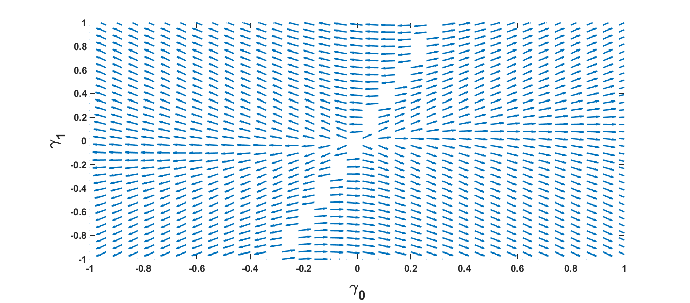
Figure 1: The RG flow of $\gamma_{0l}$ and $\gamma_{1l}$ for type-I DSMs with $w=0.3$. The fixed line $\gamma_{0}=w\gamma_{1}$ is IR unstable.

The typical RG flow of $\gamma_{0l}$ and $\gamma_{1l}$ is depicted in Fig. 1. Equations (16) and (17) have a fixed line $\gamma_{0}=w\gamma_{1}$. The RSP and $x$-RVP correspond to the lines with $\gamma_{1}=0$ and $\gamma_{0}=0$, respectively. The RG flow for the RSP and $x$-RVP are described in the followingfoot1 .

We first consider the RSP, i.e., $\gamma_{1}=0$. If we start with $\gamma_{0}>0$ and $\gamma_{1}=0$, then for $w>0$, $\gamma_{0l}$ will increase and $\gamma_{1l}$ will decrease with increasing $l$. Hence, at low energies, we get $\gamma_{0l}\rightarrow+\infty$ and $\gamma_{1l}\rightarrow-\infty$. On the other hand, if we start with $\gamma_{0}<0$ and $\gamma_{1}=0$, then for $w>0$, $\gamma_{0l}$ will decrease and $\gamma_{1l}$ will increase with increasing $l$. Hence, at low energies, we get $\gamma_{0l}\rightarrow-\infty$ and $\gamma_{1l}\rightarrow+\infty$. This means that the type-I DSM is unstable in the presence of weak RSP. Since the disorder strength becomes strong at low energies, we expect that the resulting ground state is insulating.

Next, we consider the $x$-RVP, i.e., $\gamma_{0}=0$. If we start with $\gamma_{0}=0$ and $\gamma_{1}>0$, then for $w>0$, $\gamma_{0l}$ will decrease and $\gamma_{1l}$ will increase with increasing $l$. Hence, at low energies, we get $\gamma_{0l}\rightarrow-\infty$ and $\gamma_{1l}\rightarrow+\infty$. On the other hand, if we start with $\gamma_{0}=0$ and $\gamma_{1}<0$, then for $w>0$, $\gamma_{0l}$ will increase and $\gamma_{1l}$ will decrease with increasing $l$. Hence, at low energies, we get $\gamma_{0l}\rightarrow+\infty$ and $\gamma_{1l}\rightarrow-\infty$. This means that the type-I DSM is unstable in the presence of weak $x$-RVP. Since the disorder strength becomes strong at low energies, we expect that the resulting ground state is also insulating.

The RG flow of $\lambda_{l}$ in the presence of the RSP, with various values of $\gamma_{0}$, is shown in Fig. 2. We see that $\lambda_{l}\rightarrow-\eta_{w}$ at some critical value $l_{c}$ where one of $\gamma_{0l}$ and $\gamma_{1l}$ becomes divergent. For given $w$, the value of $l_{c}$ decreases with the increasing value of $\gamma_{0}$. The situation is similar for the $x$-RVP.

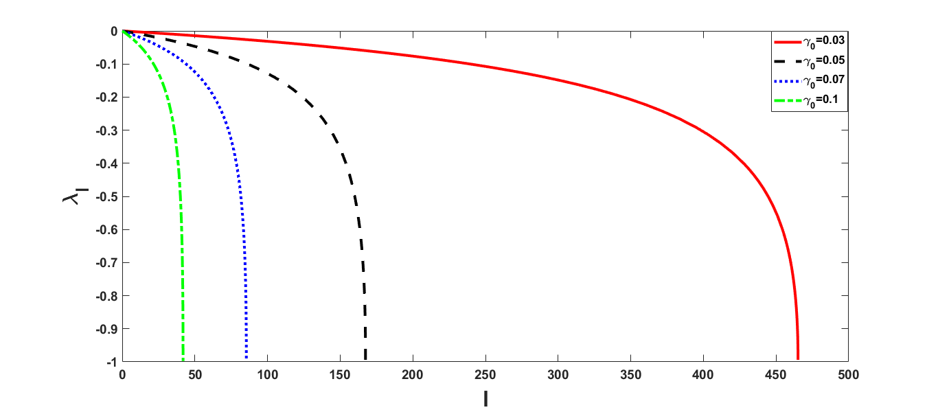
Figure 2: The RG flow of $\lambda_{l}$ for a type-I DSM in the presence of RSP ($\gamma_{1}=0=\lambda$) with $w=0.3$ and various bare values of $\gamma_{0l}$. The flow of $\lambda_{l}$ stops when one of $\gamma_{0l}$ and $\gamma_{1l}$ becomes divergent.

Although our RG scheme is different from that adopted in Ref. ZKYang, , the RG flows of the fermion-disorder couplings $\gamma_{0l}$, $\gamma_{1l}$ and the parameter $\lambda_{l}$ are similar. However, our interpretation of the resulting physics is distinct from that in Ref. ZKYang, . There, the authors consider only the kinetic energy part of the renormalized Hamiltonian and claim that the resulting phase is a DM with a bulk Fermi arc. In our opinion, this is justified only when the fermion-disorder couplings are marginal or irrelevant. Then, they can be regarded as perturbations and the kinetic energy part of the renormalized Hamiltonian dominates the low-energy physics. In the present case, the fermion-disorder couplings are relevant operators, exhibiting runaway RG flows, so that the low-energy physics is dominated by these terms. When the disorder potential becomes strong, we expect that the electrons are localized at the minia of the potential and the system is an insulator.

III.2 Type-II DSMs

Next, we consider the type-II DSMs. Similar to type-I DSMs, we find that $w^{\prime}=w$ to the one-loop order. Moreover, we choose the value of $z$ to be

$$z=1+\frac{\Delta(w-\lambda)[w(u_{0}^{2}+u_{1}^{2})-2u_{0}u_{1}]}{2\pi^{2}v_{1}v_{2}|w|(w^{2}-1)}\ ,$$ (18)

so that both $v_{1}$ and $v_{2}$ are RG invariants. Thus, we may set $v_{1}=v_{2}=v$ for simplicity. Accordingly, the one-loop RG equations for $\lambda$, $u_{1}$, and $u_{2}$ are

$$\frac{d\lambda_{l}}{dl}=(\lambda_{l}-w)[(1+w\lambda_{l})(\gamma_{0l}^{2}+\gamma_{1l}^{2})-2(w+\lambda_{l})\gamma_{0l}\gamma_{1l}]\ ,$$ (19)

and

$$\frac{d\gamma_{0l}}{dl} = (w\gamma_{0l}-\gamma_{1l})(w\gamma_{0l}^{2}-2\gamma_{0l}\gamma_{1l}+w\gamma_{1l}^{2})\ ,~{}~{}~{}~{}~{}~{}$$ (20)

$$\frac{d\gamma_{1l}}{dl} = -(w\gamma_{0l}-\gamma_{1l})(\gamma_{0l}^{2}-2w\gamma_{0l}\gamma_{1l}+\gamma_{1l}^{2})\ ,$$ (21)

where

$$\gamma_{0((1)l}=\sqrt{\frac{\Delta}{2\pi^{2}|w|(w^{2}-1)}}\frac{u_{0(1)l}}{v}\ .$$

Equations (20) and (21) have a fixed line $w\gamma_{0}=\gamma_{1}$. The typical RG flow of $\gamma_{0l}$ and $\gamma_{1l}$ is depicted in Fig. 3. We notice that the qualitative behaviors of the RG flow for $\gamma_{0l}$ and $\gamma_{1l}$ are similar for both types of DSMs. As a result, similar to type-I DSMs, the ground state is an insulator for type-II DSMs in the presence of weak RSP or $x$-RVP.

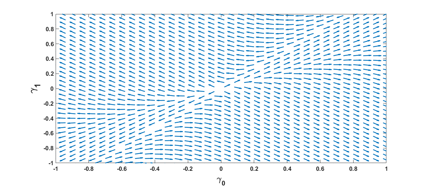
Figure 3: The RG flow of $\gamma_{0l}$ and $\gamma_{1l}$ for type-II DSMs with $w=1.3$. Notice the fixed line at $w\gamma_{0}=\gamma_{1}$.

The RG flow of $\lambda_{l}$ in the presence of the RSP, with various values of $\gamma_{0}$, is shown in Fig. 4. The qualitative behavior is similar to type-I DSMs. $\lambda_{l}\rightarrow-\eta_{w}$ at some critical value $l_{c}$ where one of $\gamma_{0l}$ and $\gamma_{1l}$ becomes divergent. For given $w$, the value of $l_{c}$ decreases with the increasing value of $\gamma_{0}$. The case with the $x$-RVP is similar. The only difference between type-I and type-II DSMs is that $l_{c}$ is smaller for the latter with the same value of $\gamma_{0}$.

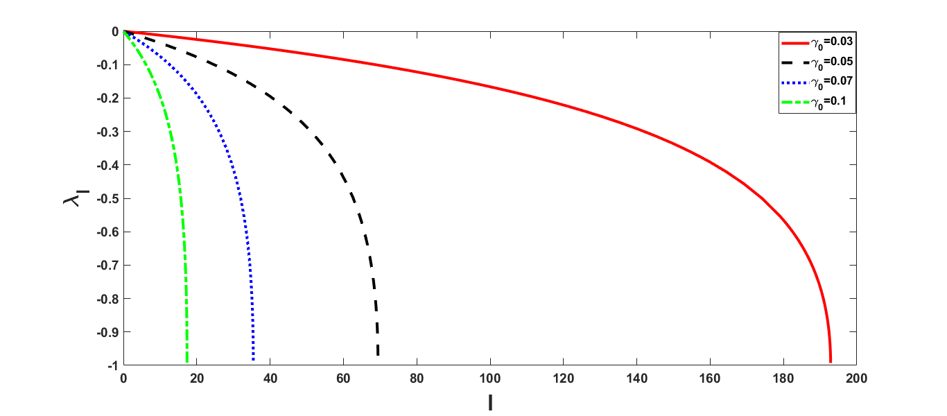
Figure 4: The RG flow of $\lambda_{l}$ for a type-II DSM in the presence of RSP ($\gamma_{1}=0=\lambda$) with $w=1.3$ and various bare values of $\gamma_{0l}$. The flow of $\lambda_{l}$ stops when one of $\gamma_{0l}$ and $\gamma_{1l}$ becomes divergent.

From the above analysis, we expect that the behaviors of the system at finite disorder strength in the regions with $|w|<1$ and $|w|>1$ are qualitatively similar to each other. That is, in the presence of the RSP or $x$-RVP, there is no phase transition from $|w|<1$ to $|w|>1$, and the ground state is an insulator. A schematic phase diagram in the presence of the RSP or $x$-RVP is shown in Fig. 5.

Figure 5: The phase diagram of a non-interacting tilted DSM in the presence of RSP or $x$-RVP. $\gamma$ and $w$ are the (dimensionless) disorder strength and the tilting parameter, respectively. I denotes the insulator. Point A located at $|w|=1$ and $\gamma=0$ is the Lifshitz transition point, separating the type-I and type-II DSMs in the absence of disorder.

IV The $y$-RVP

IV.1 Type-I DSMs

Next, we consider the $y$-RVP. For type-I DSMs, we find that $w^{\prime}=w$ to the one-loop order. If we choose

$$z=1+\frac{\Delta u_{2}^{2}}{2\pi v_{1}v_{2}(1-w^{2})^{3/2}}(1-w\lambda)\ ,$$ (22)

then $v_{1}$, $v_{2}$, and $u_{2}$ are all marginal at the one-loop order. On the other hand, the one-loop RG equation for $\lambda$ is

$$\frac{d\lambda_{l}}{dl}=\frac{\Delta u_{2}^{2}}{2\pi v_{1}v_{2}(1-w^{2})^{3/2}}(1-w\lambda_{l})(w-\lambda_{l})\ .$$ (23)

The solution of Eq. (23) with the initial value $\lambda=0$ is given by

$$\frac{\lambda_{l}-w}{\lambda_{l}-1/w}=w^{2}\exp{\!\left[-\frac{\Delta u_{2}^{2}l}{2\pi v_{1}v_{2}\sqrt{1-w^{2}}}\right]}.$$ (24)

At low energies, i.e., $l\rightarrow+\infty$, we get $\lambda_{*}=\lambda_{+\infty}=w$foot2 . Inserting this value of $\lambda_{l}$ into Eq. (22), we get a non-universal dynamical exponent $z$ given by $z=1+\eta$, where

$$\eta=\frac{\Delta u_{2}^{2}}{2\pi v_{1}v_{2}\sqrt{1-w^{2}}}\ .$$ (25)

A non-zero value of $\lambda_{*}$ will affect the dispersion relation of quasiparticles, which is determined by the poles of the single-particle propagator on the complex frequency plane with the replacement

$$v_{1(2)}\rightarrow v_{1(2)}\!\left[\frac{p}{k_{0}}\right]^{\!\eta},$$

where $p=|\bm{p}|$, $k_{0}\sim 1/a_{0}$, and $a_{0}$ is the lattce spacing. As a result, the dispersion relation of the quasiparticles is given by

$$E_{\pm}(\bm{p})=\pm\!\left(\frac{p}{k_{0}}\right)^{\!\eta}\!\sqrt{v_{1}^{2}p_{1}^{2}+\frac{v_{2}^{2}}{1-w^{2}}p_{2}^{2}}\ .$$ (26)

To sum up, in the presence of weak $y$-RVP, the system is a SM with $z>1$ and the fermion-disorder coupling is marginal.

For a SM, various physical quantities will exhibit power-law temperature dependence at low temperatures. This has been discussed in Ref. ZKYang, , and we will not duplicate it here. Instead, we ask the question. Will this SM be stable against the presence of a marginal fermion-disorder coupling? As is well known, the disorder potential is a marginal perturbation to the FL, and a $2$D FL is unstable toward an insulator even in the presence of an arbitrarily weak disorder potentialAbrahams . To answer this question, we employ the replica trick to map the renormalized action into a replica field theory and then perform a mean-field analysis.

The disorder-averaged replicated partition function $\mathcal{Z}$ in the imaginary-time formulation is given byFinkelshtein ; Belitz ; Altland

$$\mathcal{Z}=\!\int\!D[A]P[A]\!\int\!D[\chi]D[\bar{\chi}]e^{-S_{0}-S_{i}}\ ,$$

where

$$S_{0} = \!\sum_{a=1}^{M}\!\sum_{\xi,n}\!\int\!d^{2}x\bar{\chi}_{\xi na}[-i\omega_{n}(1+w\sigma_{1})+\hat{h}_{\xi}]\chi_{\xi na}$$

$$= \!\sum_{\xi,n}\!\int\!d^{2}x\bar{\psi}_{\xi n}[-i\omega_{n}(1+w\sigma_{1})+\hat{h}_{\xi}]\otimes I_{M}\psi_{\xi n}\ ,$$

$$S_{i} = -u_{2}\!\sum_{a=1}^{M}\!\sum_{\xi,n}\!\int\!d^{2}x\bar{\chi}_{\xi na}\sigma_{2}\chi_{\xi na}A$$

$$= -u_{2}\!\sum_{\xi,n}\!\int\!d^{2}x\bar{\psi}_{\xi n}\sigma_{2}\otimes I_{M}\psi_{\xi n}A\ ,$$

and

$$P[A]=\exp{\!\left(-\frac{1}{2\Delta}\!\int\!d^{2}xA^{2}\right)}.$$

In the above, $\omega_{n}=(2n+1)\pi T$, $a$ is the replica index, $I_{M}$ is the unit matrix of dimension $M$ in the replica space, $\psi_{\xi n}=[\chi_{\xi n1},\cdots,\chi_{\xi nM}]^{t}$, $\bar{\psi}_{\xi n}=[\bar{\chi}_{\xi n1},\cdots,\bar{\chi}_{\xi nM}]$, and

$$\hat{h}_{\xi}=v\!\left(\frac{p}{k_{0}}\right)^{\!\eta}\![\xi(w+\sigma_{1})p_{1}+\sigma_{2}p_{2}]\ ,$$

in the momentum space. For simplicity, we have set $v_{1}=v=v_{2}$ and dropped out the spin index $\sigma$. By integrating out the random field $A(\bm{r})$, $\mathcal{Z}$ can be written as

$$\mathcal{Z}=\!\int\!\!D[\chi]D[\bar{\chi}]\exp{\!\left[-S_{0}+\frac{g_{2}^{2}}{2}\!\!\int\!\!d^{2}x(\bar{\Psi}\Gamma\Psi)^{2}\right]},$$

where $g_{2}=\sqrt{\Delta u_{2}^{2}}$, $\Psi=[\Psi_{1},\Psi_{-1}]^{t}$, $\bar{\Psi}=[\bar{\Psi}_{1},\bar{\Psi}_{-1}]$, $\Gamma_{mn;\xi\xi^{\prime}}^{ab}=\delta_{mn}\delta_{ab}\delta_{\xi\xi^{\prime}}\sigma_{2}$, and

$$\Psi_{\xi} = [\cdots,\psi_{\xi 1},\psi_{\xi 0},\psi_{\xi-1},\cdots]^{t}\ ,$$

$$\bar{\Psi}_{\xi} = [\cdots,\bar{\psi}_{\xi 1},\bar{\psi}_{\xi 0},\bar{\psi}_{\xi-1},\cdots]\ .$$

To proceed, we make a Hubbard-Stratonovich transformation on the four-fermion coupling arising from the integration over the random field:

$$\!\!\exp{\!\left[\frac{g_{2}^{2}}{2}\!\!\int\!\!d^{2}x(\bar{\Psi}\Gamma\Psi)^{2}\right]}$$

$$\!\!=\!\int\!\!D[Q]\exp{\!\left\{-\!\int\!\!d^{2}x\!\left[\frac{1}{2}\mbox{tr}Q^{2}-ig_{2}\bar{\Psi}Q\Gamma\Psi\right]\!\right\}},$$

where $Q^{\dagger}=Q$. If we put an UV cutoff on the frequencies, i.e., $-R\leq n<R$ or $|\omega_{n}|\leq(2R-1)\pi T$, then the symmetry group in the absence of the frequency term is U($2RM$). Under the U($2RM$) transformation,

$$\Psi_{\xi}\rightarrow U\Psi_{\xi}\ ,~{}~{}\bar{\Psi}_{\xi}\rightarrow\bar{\Psi}_{\xi}U^{\dagger}\ ,$$ (27)

the $Q$ field transforms as

$$Q_{\xi\xi^{\prime}}\rightarrow UQ_{\xi\xi^{\prime}}U^{\dagger}\ .$$ (28)

By integrating out the fermion fields, $\mathcal{Z}$ can be written as

$$\mathcal{Z}=\!\int\!\!D[Q]e^{-I[Q]}\ ,$$ (29)

where

$$I[Q] = -\mbox{tr}\ln{\!\left[i\hat{\omega}(1+w\sigma_{1})-\hat{h}+ig_{2}Q\Gamma\right]}$$ (30)

$$+\frac{1}{2}\!\int\!\!d^{2}x\mbox{tr}Q^{2}.$$

In Eq. (30), $\hat{\omega}_{mn;\xi\xi^{\prime}}^{ab}=\omega_{n}\delta_{mn}\delta_{ab}\delta_{\xi\xi^{\prime}}$ and $\hat{h}_{mn;\xi\xi^{\prime}}^{ab}=\hat{h}_{\xi}\delta_{mn}\delta_{ab}\delta_{\xi\xi^{\prime}}$.

We assume that the path integral is dominated by configurations of the $Q$ field close to the homogeneous solution $Q_{0}$ of the saddle-point equation $\delta I[Q]/\delta Q=0$. It is given by

$$Q_{0}=ig_{2}\!\int\!\frac{d^{2}p}{(2\pi)^{2}}\mbox{tr}[\Gamma\hat{G}(i\omega_{n},\bm{p})]\ ,$$ (31)

where the trace is taken over the spinor space which describes the conduction-valence band degrees of freedom and

$$\hat{G}^{-1}(i\omega_{n},\bm{p})=i\hat{\omega}(1+w\sigma_{1})-\hat{h}+ig_{2}Q_{0}\Gamma\ .$$ (32)

To solve Eq. (31), we try the ansatz $g_{2}Q_{\xi\xi^{\prime}}=\alpha_{\xi}\Lambda\delta_{\xi\xi^{\prime}}$, where $\Lambda_{mn}^{ab}=s_{n}\delta_{mn}\delta_{ab}$, $s_{n}=\mbox{sgn}(\omega_{n})$, and $\alpha_{\xi}$ is a real constant which may depend on the valley index $\xi$. Then, $\alpha_{\xi}$ satisfies the equation

$$\alpha_{\xi} = \!\int_{|p_{i}|<k_{0}}\!\frac{d^{2}p}{(2\pi)^{2}}\frac{2ig_{2}^{2}/v^{2}[i\alpha_{\xi}-s_{n}v(p/k_{0})^{\eta}p_{2}]}{(1-w^{2})(p/k_{0})^{2\eta}p_{1}^{2}+[(p/k_{0})^{\eta}p_{2}-is_{n}\alpha_{\xi}/v]^{2}}$$

$$= \!\int_{|p_{i}|<k_{0}}\!\frac{d^{2}p}{(2\pi)^{2}}\frac{2ig_{2}^{2}/v^{2}[i\alpha_{\xi}-v(p/k_{0})^{\eta}p_{2}]}{(1-w^{2})(p/k_{0})^{2\eta}p_{1}^{2}+[(p/k_{0})^{\eta}p_{2}-i\alpha_{\xi}/v]^{2}}\ .$$

In the above, we have taken the limit $\omega_{n}\rightarrow 0$. Moreover, we have changed the variable $s_{n}p_{2}\rightarrow s_{n}p_{2}$. The momentum integral is divergent, and an UV cutoff $k_{0}$ in momenta is introduced. We notice that this equation has real solutions. Furthermore, $\alpha_{\xi}$ is independent of $\xi$, and thus we will set $\alpha_{\xi}\rightarrow\alpha$. Defining the dimensionless quantity $\tilde{\alpha}=\alpha/(vk_{0})$, the above equation becomes

$$\tilde{\alpha}=\!\int_{\mathcal{D}}\!\frac{d^{2}x}{(2\pi)^{2}}\frac{2ig_{2}^{2}/v^{2}(i\tilde{\alpha}-r^{\eta}x_{2})}{(1-w^{2})r^{2\eta}x_{1}^{2}+(r^{\eta}x_{2}-i\tilde{\alpha})^{2}}\ ,$$ (33)

where $r=\sqrt{x_{1}^{2}+x_{2}^{2}}$ and $\mathcal{D}=\{(x_{1},x_{2})||x_{1}|,|x_{2}|\leq 1\}$. Equation (33) has a trivial solution $\tilde{\alpha}=0$. We would like to search for a non-trivial real solution if it exists. It is clear that if $\tilde{\alpha}$ is a solution of Eq. (33), then $-\tilde{\alpha}$ is also a solution. Without loss of generality, we take $\tilde{\alpha}\geq 0$.

To find a non-trivial real solution of Eq. (33), we add the complex conjugate of this equation to itself, yielding

$$\tilde{\alpha}=\!\int_{\mathcal{D}}\!\frac{d^{2}x}{(2\pi)^{2}}\frac{2g_{2}^{2}/v^{2}\tilde{\alpha}[r^{2\eta}x_{2}^{2}+\tilde{\alpha}^{2}-(1-w^{2})r^{2\eta}x_{1}^{2}]}{[(1-w^{2})r^{2\eta}x_{1}^{2}+r^{2\eta}x_{2}^{2}-\tilde{\alpha}^{2}]^{2}+4r^{2\eta}x_{2}^{2}\tilde{\alpha}^{2}}\ .$$

Now the right hand side of this equation becomes real. Therefore, a non-trivial solution satisfies this equation

$$1=\frac{4t}{\pi}\!\int^{1}_{0}\!\!dx_{1}dx_{2}\frac{r^{2\eta}x_{2}^{2}+\tilde{\alpha}^{2}-(1-w^{2})r^{2\eta}x_{1}^{2}}{[(1-w^{2})r^{2\eta}x_{1}^{2}+r^{2\eta}x_{2}^{2}-\tilde{\alpha}^{2}]^{2}+4r^{2\eta}x_{2}^{2}\tilde{\alpha}^{2}}\ ,$$ (34)

where $t=g_{2}^{2}/(2\pi v^{2})$ measures the disorder strength and $\eta=t/\sqrt{1-w^{2}}$. Since $vk_{0}$ can be regarded as the largest energy scale in this problem, we must have $\tilde{\alpha}<1$.

Figure 6: The behavior of $I(s)$ in the range $0\leq s\leq 1$ for different values of $t$ with $|w|=0.3$, where $s=\tilde{\alpha}^{2}$. For reference, $I(s)=1$ is indicated by the dotted line.

We shall solve Eq. (34) graphically. Let us define the right hand side of Eq. (34) as a function of $s=\tilde{\alpha}^{2}$:

$$\!\!I(s)$$

$$\!\!=\!\!\int^{1}_{0}\!\!dx_{1}dx_{2}\frac{(4t/\pi)[s+r^{2\eta}x_{2}^{2}-(1-w^{2})r^{2\eta}x_{1}^{2}]}{[(1-w^{2})r^{2\eta}x_{1}^{2}+r^{2\eta}x_{2}^{2}-s]^{2}+4sr^{2\eta}x_{2}^{2}}\ .$$

Figure 6 shows the function $I(s)$ in the range $0\leq s\leq 1$ for different values of $t$ with $|w|=0.3$. We see that for given $|w|$, there exists a critical value $t_{c}(|w|)$ such that we get a nontrivial solution of $\tilde{\alpha}$ when $t>t_{c}(|w|)$. On the other hand, there is only a trivial solution $\tilde{\alpha}=0$ when $t<t_{c}(|w|)$. Moreover, for a fixed value of $|w|$, the nontrivial solution $\tilde{\alpha}$, if it exists, is an increasing function of $t$.

The mean-field solution with $\tilde{\alpha}\neq 0$ has a nonvanishing spectral density at the Fermi level, and thus corresponds to the DM phase. Since the U($2RM$) symmetry is broken down to U($RM$)$\times$U($RM$) when $\tilde{\alpha}\neq 0$, there will be Goldstone modes according to the Goldstone theorem. The DM phase is stable only when it survives the fluctuations of these Goldstone modes. The latter is described by a certain type of generalized non-linear $\sigma$ models. The RG analysis of the generalized non-linear $\sigma$ model indicates that the DM phase in $d=2$ is unstable toward an insulatorHikami . On the other hand, the mean-field solution with $\tilde{\alpha}=0$ corresponds to the SM phase with $z>1$. It is stable against small fluctuations around the mean-field state due to the vanishing DOS at the Fermi level. Hence, we claim that the SM phase with $z>1$ is stable against the weak $y$-RVP when $t<t_{c}(|w|)$.

For given $|w|$, the critical value $t_{c}(|w|)$ is determined by setting $\tilde{\alpha}=0$ in Eq. (34), yielding

$$1=\frac{4t}{\pi}\!\int^{1}_{0}\!\!dx_{1}dx_{2}\frac{r^{2\eta}x_{2}^{2}-(1-w^{2})r^{2\eta}x_{1}^{2}}{[(1-w^{2})r^{2\eta}x_{1}^{2}+r^{2\eta}x_{2}^{2}]^{2}}\ .$$ (35)

Equation (35) can be solved numerically, and the result is shown in Fig. 7. We see that $t_{c}$ is a monotonously decreasing function of $|w|$. Moreover, $t_{c}\rightarrow 0$ as $|w|\rightarrow 1$.

Figure 7: The critical (dimensionless) disorder strength $t_{c}$ as a function of $|w|$ in the range $0\leq|w|<1$.

IV.2 Type-II DSMs

Now we consider the type-II DSMs. To the one-loop order, we find that $w^{\prime}=w$. It we choose $z$ to be

$$z=1+\frac{\Delta u_{2}^{2}w(w-\lambda)}{2\pi^{2}v_{1}v_{2}|w|(w^{2}-1)}w(w-\lambda)\ ,$$ (36)

then both $v_{1}$ and $v_{2}$ are RG invariants, and

$$\lambda^{\prime} = \lambda+\frac{\Delta u_{2}^{2}(1-w\lambda)(w-\lambda)}{2\pi^{2}v_{1}v_{2}|w|(w^{2}-1)}l+O(\lambda^{2})\ ,$$

$$u_{2}^{\prime} = u_{2}+\frac{\Delta u_{2}^{3}}{2\pi^{2}v_{1}v_{2}|w|}l+O(\lambda^{2})\ .$$

As a result, $w$ and $v_{1,2}$ are marginal to the one-loop order. On the other hand, the one-loop RG equations for $\lambda$ and $u_{2}$ are

$$\frac{d\lambda_{l}}{dl} = \frac{\gamma_{2l}(1-w\lambda)(w-\lambda)}{2(w^{2}-1)}\ ,$$ (37)

$$\frac{d\gamma_{2l}}{dl} = \gamma_{2l}^{2}\ ,$$ (38)

where $\gamma_{2l}=\frac{\Delta}{|w|\pi^{2}}(u_{2l}/v)^{2}$ and for simplicity, we have set $v_{1}=v=v_{2}$. From Eq. (38), we see that the $u_{2}$ term is a relevant perturbation. That is, the pure type-II DSM is unstable in the presence of weak $y$-RVP, and the ground state is supposed to be an insulator. This is in contrast with type-I DSMs in the presence of weak $y$-RVP. Consequently, we expect the occurrence of a QPT upon varying the value of $|w|$ for a given disorder strength. A schematic phase diagram in the presence of $y$-RVP is shown in Fig. 8. The phase boundary between the SM and insulator is obtained from Fig. 7. According to the mean-field theory, the SM-insulator transition is continuous.

Figure 8: The schematic phase diagram of a non-interacting tilted DSM in the presence of $y$-RVP. $\gamma$ and $w$ are the (dimensionless) disorder strength and the tilting parameter, respectively. Point A located at $|w|=1$ and $\gamma=0$ is the Lifshitz transition point, separating the type-I and type-II DSMs in the absence of disorder.

V The RM

V.1 Type-I DSMs

Finally, we consider the RM. To the one-loop order, we find that $w^{\prime}=w$. If we choose $z$ to be

$$z=1+\frac{\Delta u_{3}^{2}}{2\pi v_{1}v_{2}(1-w^{2})^{3/2}}(1-w\lambda)\ ,$$ (39)

then both $v_{1}$ and $v_{2}$ are RG invariants, and

$$\lambda^{\prime} = \lambda+\frac{\Delta u_{3}^{2}}{2\pi v^{2}(1-w^{2})^{3/2}}(1-w\lambda)(w-\lambda)l$$

$$+O(l^{2})\ ,$$

$$u_{3}^{\prime} = u_{3}-\frac{\Delta u_{3}^{3}}{2\pi v^{2}\sqrt{1-w^{2}}}l+O(l^{2})\ .$$

In the last two equations, we have set $v_{1}=v_{2}=v$ for simplicity. Hence, the one-loop RG equations for $\lambda$ and $u_{3}$ are given by

$$\frac{d\lambda_{l}}{dl}=\frac{\Delta u_{3}^{2}}{2\pi v^{2}(1-w^{2})^{3/2}}(1-w\lambda_{l})(w-\lambda_{l})\ ,$$ (40)

and

$$\frac{du_{3l}}{dl}=-\frac{\Delta u_{3l}^{3}}{2\pi v^{2}\sqrt{1-w^{2}}}\ ,$$ (41)

respectively. Equation (41) has only one fixed point $u_{3}=0$, with $z=1$. Since the right hand side in Eq. (41) is negative, this fixed point is IR stable. In other words, the RM term is marginally irrelevant at weak disorder. Consequently, the type-I DSM is stable against the weak RM disorder.

To determine the fate of $\lambda_{l}$, we have to solve Eqs. (40) and (41). By introducing the dimensionless coupling $\gamma_{3l}=\frac{\Delta}{\pi\sqrt{1-w^{2}}}(u_{3l}/v)^{2}$, the solution with the bare value $\lambda=0$ is

$$\frac{\lambda_{l}-w}{\lambda_{l}-1/w}=\frac{w^{2}}{\sqrt{1+\gamma_{3}l}}\ .$$ (42)

From Eq. (42), we find that $\lambda_{*}=\lambda_{+\infty}=w$. Using this value of $\lambda_{l}$, the dispersion relation of quasiparticles near the Dirac point is given by

$$E_{\pm}(\bm{p})=\pm\sqrt{v_{1}^{2}p_{1}^{2}+\frac{v_{2}^{2}}{1-w^{2}}p_{2}^{2}}\ .$$ (43)

We see that the quasiparticles can be described by the Dirac fermions with an untilted and anisotropic Dirac cone. This is consistent with Ref. ZKYang, .

To sum up, the ground state at $|w|<1$ in the presence of a weak RM disorder is an untilted DSM with an anisotropic Dirac cone. Since the fermion-disorder coupling is marginally irrelevant, the physical quantities may acquire logarithmic temperature dependence at low temperatures.

V.2 Type-II DSMs

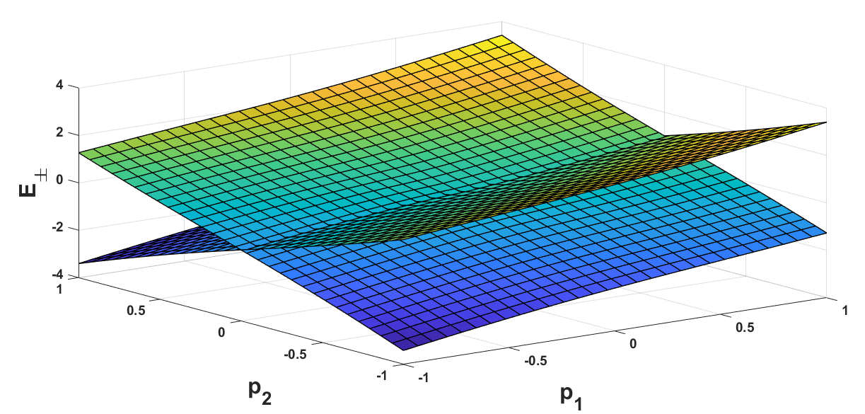
Figure 9: The dispersion relations $E_{\pm}(\bm{p})$ of quasiparticles around a Dirac node with the valley index $\xi=1$ in a type-II DSM in the presence of RM, with $w=1.1$ and $z=1.2$. $E_{\pm}(\bm{p})$ are measured in units of $|w|vk_{0}$ and the momentum $\bm{p}$ is measured in units of $k_{0}$. For simplicity, we have set $v_{1}=v=v_{2}$.

Now we consider type-II DSMs. To the one-loop order, we find that $w^{\prime}=w$. If we choose $z$ to be

$$z=1+\frac{\Delta u_{3}^{2}w(w-\lambda)}{2\pi^{2}v_{1}v_{2}|w|(w^{2}-1)}\ ,$$ (44)

then we get $v_{1,2}^{\prime}=v_{1,2}$, $u_{3}^{\prime}=u_{3}$, and

$$\lambda^{\prime}=\lambda+\frac{\Delta u_{3}^{2}(1-w\lambda)(w-\lambda)}{2\pi^{2}v_{1}v_{2}|w|(w^{2}-1)}l+O(\lambda^{2})\ .$$

As a result, $w$, $v_{1,2}$, and $u_{3}$ are all marginal to the one-loop order. On the other hand, the one-loop RG equation for $\lambda$ is

$$\frac{d\lambda_{l}}{dl}=\frac{\Delta u_{3}^{2}(1-w\lambda)(w-\lambda)}{2\pi^{2}v_{1}v_{2}|w|(w^{2}-1)}\ .$$ (45)

The solution of Eq. (45) with the initial value $\lambda=0$ is

$$\frac{\lambda_{l}-1/w}{\lambda_{l}-w}=\frac{1}{w^{2}}\exp{\!\left(-\frac{\Delta u_{3}^{2}l}{2\pi^{2}v_{1}v_{2}|w|}\right)}.$$ (46)

Hence, we get $\lambda_{*}=\lambda_{+\infty}=1/w$. Inserting this value of $\lambda_{l}$ into Eq. (44), we obtain the dynamical exponent $z=1+\eta$, where

$$\eta=\frac{\Delta u_{3}^{2}}{2\pi^{2}v_{1}v_{2}|w|}\ .$$ (47)

For $\lambda=\lambda_{*}$, the dispersion relation of quasiparticles is

$$E_{\pm}(\bm{p})=w\!\left(\frac{p}{k_{0}}\right)^{\!\eta}\!\!\left(\xi v_{1}p_{1}\pm\frac{v_{2}}{\sqrt{w^{2}-1}}p_{2}\right),$$ (48)

and $k_{0}\sim 1/a_{0}$. A typical form of $E_{\pm}(\bm{p})$ is plotted in Fig. 9. We see that the quasiparticles at low energies are not described by the Dirac fermions anymore. However, it is still a FL with an open Fermi surface given by

$$p_{2}=\pm\xi\sqrt{w^{2}-1}(v_{1}/v_{2})p_{1}\ ,$$ (49)

which consists of two straight lines for each valley.

To determine the fate of this FL in the presence of a weak marginal fermion-disorder coupling, we determine the physical properties in terms of the perturbation theory. This is valid when the disorder strength is weak since the fermion-disorder coupling is marginal. In particular, we calculate the one-loop fermion self-energy:

$$\Sigma_{\xi\sigma}(ip_{0}) = -\Delta u_{3}^{2}\!\int\!\!\frac{d^{2}p}{(2\pi)^{2}}\frac{ip_{0}-\xi wv(p/k_{0})^{\eta}p_{1}}{[p_{0}+i\xi wv(p/k_{0})^{\eta}p_{1}]^{2}+[-ip_{0}/w+\xi v(p/k_{0})^{\eta}p_{1}]^{2}+v^{2}(p/k_{0})^{2\eta}p^{2}_{2}}$$

$$-\Delta u_{3}^{2}\sigma_{1}\!\int\!\!\frac{d^{2}p}{(2\pi)^{2}}\frac{ip_{0}/w-\xi v(p/k_{0})^{\eta}p_{1}}{[p_{0}+i\xi wv(p/k_{0})^{\eta}p_{1}]^{2}+[-ip_{0}/w+\xi v(p/k_{0})^{\eta}p_{1}]^{2}+v^{2}(p/k_{0})^{2\eta}p^{2}_{2}}\ .$$

By analytic continuation $ip_{0}\rightarrow p_{0}+i0^{+}$, the retarded slef-energy $\Sigma^{r}_{\xi\sigma}(p_{0})$ is given by

$$\Sigma^{r}_{\xi\sigma}(p_{0}) = \frac{\Delta u_{3}^{2}k_{0}}{8\pi^{2}v(1-1/w^{2})}\!\left(1+\frac{\sigma_{1}}{w}\right)\!\!\int\!\!d^{2}x\frac{1}{\tilde{p}_{0}-\xi wr^{\eta}x_{1}-\sqrt{\frac{w^{2}}{w^{2}-1}}r^{\eta}x_{2}+i0^{+}}$$

$$+\frac{\Delta u_{3}^{2}k_{0}}{8\pi^{2}v(1-1/w^{2})}\!\left(1+\frac{\sigma_{1}}{w}\right)\!\!\int\!\!d^{2}x\frac{1}{\tilde{p}_{0}-\xi wr^{\eta}x_{1}+\sqrt{\frac{w^{2}}{w^{2}-1}}r^{\eta}x_{2}+i0^{+}}\ ,$$

where $x_{i}=p_{i}/k_{0}$ with $i=1,2$, $r=\sqrt{x_{1}^{2}+x_{2}^{2}}$, and $\tilde{p}_{0}=p_{/}(vk_{0})$. For simplicity, we have set $v_{1}=v=v_{2}$. As a result, its imaginary part is of the form

$$\mbox{Im}\Sigma^{r}_{\xi\sigma}(p_{0}) = -\frac{\Delta u_{3}^{2}k_{0}}{8\pi v(1-1/w^{2})}\!\left(1+\frac{\sigma_{1}}{w}\right)\!\!\int\!\!d^{2}x\delta\!\left(\tilde{p}_{0}-\xi wr^{\eta}x_{1}-\sqrt{\frac{w^{2}}{w^{2}-1}}r^{\eta}x_{2}\right)$$

$$-\frac{\Delta u_{3}^{2}k_{0}}{8\pi v(1-1/w^{2})}\!\left(1+\frac{\sigma_{1}}{w}\right)\!\!\int\!\!d^{2}x\delta\!\left(\tilde{p}_{0}-\xi wr^{\eta}x_{1}+\sqrt{\frac{w^{2}}{w^{2}-1}}r^{\eta}x_{2}\right).$$

Setting $\tilde{p}_{0}=0$, we find that

$$\mbox{Im}\Sigma^{r}_{\xi\sigma}(0) = -\frac{\Delta u_{3}^{2}k_{0}|w|}{8\pi v(w^{2}-1)}\!\left(1+\frac{\sigma_{1}}{w}\right)\!\!\int\!\!d^{2}x\frac{1}{r^{\eta}}\delta\!\left(x_{1}+\frac{\eta_{w}\xi}{\sqrt{w^{2}-1}}x_{2}\right)$$

$$-\frac{\Delta u_{3}^{2}k_{0}|w|}{8\pi v(w^{2}-1)}\!\left(1+\frac{\sigma_{1}}{w}\right)\!\!\int\!\!d^{2}x\frac{1}{r^{\eta}}\delta\!\left(x_{1}-\frac{\eta_{w}\xi}{\sqrt{w^{2}-1}}x_{2}\right)$$

$$= -\frac{\Delta u_{3}^{2}k_{0}|w|^{1-\eta}}{2\pi v(w^{2}-1)^{1-\eta/2}}\!\left(1+\frac{\sigma_{1}}{w}\right)\!\!\int^{+\infty}_{0}\!\frac{dx_{2}}{x_{2}^{\eta}}\ .$$

Since $\eta<1$ for the weak disorder strength, the integral is UV divergent. We have to cut it off at a scale $D/(vk_{0})$ where $D=O(vk_{0})$ is the band width. Without loss of generality, we choose $D=vk_{0}$. (A different choice of the ratio $D/(vk_{0})$ corresponds to the redefinition of the bare value $u_{3}^{2}$.) Thus, we have

$$\mbox{Im}\Sigma^{r}_{\xi\sigma}(0) = -\frac{\Delta u_{3}^{2}k_{0}|w|^{1-\eta}}{2\pi v(w^{2}-1)^{1-\eta/2}}\!\left(1+\frac{\sigma_{1}}{w}\right)\!\!\int^{1}_{0}\!\frac{dx_{2}}{x_{2}^{\eta}}$$

$$= -\frac{\Delta u_{3}^{2}k_{0}|w|^{1-\eta}}{2\pi v(1-\eta)(w^{2}-1)^{1-\eta/2}}\!\left(1+\frac{\sigma_{1}}{w}\right).$$

This result implies that to the one-loop order, the single-particle Green function for quasiparticles at low frequencies and small momenta is of the form

$$G_{\xi}^{-1}(P) = \!\left(1+\frac{\sigma_{1}}{w}\right)\!\!\left[-ip_{0}+\xi v\!\left(\frac{p}{k_{0}}\right)^{\!\eta}\!p_{1}-\frac{\mbox{sgn}(p_{0})}{2\tau}\right]$$ (50)

$$+v\!\left(\frac{p}{k_{0}}\right)^{\!\eta}\!p_{2}\sigma_{2}\ ,$$

in the imaginary-time formulation, where the mean free time $\tau$ is given by

$$\frac{1}{\tau}=\frac{\Delta u_{3}^{2}k_{0}|w|^{1-\eta}}{\pi v(1-\eta)(w^{2}-1)^{1-\eta/2}}\ .$$ (51)

Since the quasiparticles acquire a nonzero mean free time, the system is a DM at weak disorder strength. According to the scaling theory of localizationAbrahams , a DM phase in $d=2$ is unstable in the presence of weak disorder and turns into an insulator. Alternatively, we can investigate the role of the marginal fermion-disorder coupling by a replica mean-field theory, similar to what we have done for type-I DSMs in the presence of $y$-RVP. The above perturbative calculation suggests that the mean-field equation always has a non-zero solution such that the quasiparticles acquire a nonvanishing mean free time. The fluctuations around this broken-symmetry solution are described by a generalized nonlinear $\sigma$ model. In two dimensions, the nonlinear $\sigma$ model has only one phase – the disordered phase, corresponding to the insulator within the present context. In any case, we reach the conclusion that the ground state is insulating for $|w|>1$.

Since the system with $|w|<1$ is an untilted DSM at weak disorder strength and insulating when $|w|>1$, we conclude that there is a QPT from $|w|<1$ to $|w|>1$ for a given disorder strength in the presence of weak RM. The resulting schematic phase diagram is shown in Fig. 10. In fact, as we approach the phase boundary between the DSM and the insulating phase from the side of the DSM, the component of the velocity perpendicular to the tilting direction (the $y$-direction in the present setup) becomes singular at the phase boundary. On the other hand, if we approach the phase boundary from the side of the insulator, we find that $1/\tau\rightarrow+\infty$ at the phase boundary. All these imply that the quantum fluctuations are strong around the line $|w|=1$ and the starting point we have adopted, i.e., starting from either $|w|<1$ or $|w|>1$ may not be appropriate. As a result, Fig. 10 is just schematic, and the exact location of the phase boundary may not be a straight line. Moreover, other phases may exist close to the $|w|=1$ line.

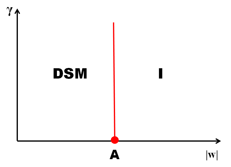
Figure 10: The schematic phase diagram of a non-interacting tilted DSM in the presence of weak RM. $\gamma$ and $w$ are the (dimensionless) disorder strength and the tilting parameter, respectively. Point A located at $|w|=1$ and $\gamma=0$ is the Lifshitz transition point, separating the type-I and type-II DSMs in the absence of disorder. The phase boundary between the DSM and insulating phase is schematic. When the disorder strength is further increased, the DSM will turn into an insulator.

VI Conclusions and discussions

We study the effects of various types of quenched disorder on the non-interacting tilted Dirac fermions in two dimensions with the help of the perturbative RG. Since the RG transformations must scale to the Fermi surface, we parametrize the low-energy degrees of freedom according to their energies so that we can integrate out the modes with large energies properly. When the Fermi surface is point-like, the results are consistent with those by integrating out the modes with large momenta. On the other hand, the answers may be different when the Fermi surface is extended. Although we focus on the $2$D tilted DSMs, it is straightforward ro extend our method to the tilted WSMs in three dimensions.

The relevancy of various fermion-disorder couplings under the RG transformations in both types of DSMs to the one-loop order is summarized in Table 1. Whenever the fermion-disorder coupling is relevant, we extrapolate our one-loop RG equations to the strong disorder regime and claim that the resulting phase is an insulator. When the fermion-disorder coupling is marginal, we examine its role by using either the mean-field approximation of a replica field theory or the first-order Born approximation. If the fermion-disorder coupling is irrelevant, then this phase is stable against the presence of weak disorder.

When $w\neq 0$, the RSP and the $x$-RVP will generate each other under the RG transformations even if one of the bare value is zero. Hence, we must consider them together when calculating the RG equations. In the presence of the RSP or the $x$-RVP, we find that both types of DSMs become insulators even at weak disorder strength because the corresponding fermion-disorder coupling flows to strong disorder regime.

disorder	type-I	type-II
RSP	relevant	relevant
$x$-RVP	relevant	relevant
$y$-RVP	marginal	relevant
RM	irrelevant	marginal

Table 1: The relevancy of various fermion-disorder couplings under the RG transformations in both types of DSMs to the one-loop order.

For the $y$-RVP, we find that the system at $|w|<1$ is a SM characterized by a non-universal dynamical exponent $z>1$. This SM is fragile since it becomes an insulator at a moderate strength of disorder. Especially, the critical disorder strength vanishes as $|w|\rightarrow 1$. On the other hand, the system is insulating at $|w|>1$. Thus, we expect that there is a SM-insulator transition upon varying $|w|$ for a given disorder strength, which is continuous according to our replica mean-field theory. The calculations of the critical exponents associated with this transition are beyond the scope of the present work.

For the weak RM, the system at $|w|<1$ is an untilted DSM with an anisotropic Dirac cone. On the other hand, it is an insulator when $|w|>1$. Thus, we expect that there is a DSM-insulator transition upon varying $|w|$ for a given disorder strength. The determination of the nature of this transition is beyond the scope of the present work. Moreover, on account of the strong fluctuations close to the $|w|=1$ line, our approach which starts from either side may fail, and there can exist other phases near the $|w|=1$ line.

For type-I DSMs, the effects of the quenched disorder have been studied with a different type of RG schemeZKYang . For the $y$-RVP and RM, the phases we find at the weak disorder are identical to the ones in Ref. ZKYang, . For the former, we indicate that the SM may be unstable upon increasing the disorder strength, which has not been examined in Ref. ZKYang, . We further determine the critical disorder strength beyond which the SM becomes unstable toward an insulator. The main difference between our work and Ref. ZKYang, lies on the nature of the ground state of type-I DSMs in the presence of RSP or $x$-RVP. According to Ref. ZKYang, , the ground state is a DM with a bulk Fermi arc. This DM cannot be stable since the fermion-disorder coupling flows to the strong disorder regime at low energies. One possibility in the strong disorder regime is an insulating phase due to the random potential scattering.

Further studies, maybe numerics, are warranted to justify the phase diagrams we have obtained in this work. In particular, the nature of the DSM-insulator transition and the phases close to the transition line in the presence of a weak RM are open questions. Since electrons carry electric charges, the long-range Coulomb interaction is always present. It is interesting to investigate how the electron-electron interactions affect the phase diagrams. For type-I DSMs, this question has been studied in Ref. ZKYang, . For type-II DSMs, however, this question remains unanswered.

Appendix A Derivation of the one-loop RG equations

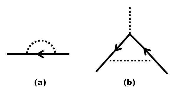
Figure 11: The one-loop correction to the self-energy of Dirac fermions (a) and the fermion-disorder coupling (b). The solid and the dashed lines correspond to the fermion propagator and the disorder potential, respectively.

Here we present the details of the derivation of the one-loop RG equations. To properly integrate out the modes with large energies, we have parametrized the low-energy degrees of freedom according to their energies, as shown in Eqs (11) and (12) for type-I and type-II DSMs, respectively. In terms of them, we write the involved momentum integrals as

$$\!\int\!d^{2}\tilde{p}\!\! = \!\!\frac{1}{2}\!\int^{\Lambda}_{0}\!\frac{EdE}{(1-w^{2})^{3/2}}\!\int^{2\pi}_{0}\!\!d\theta(1-\xi w\cos{\theta})$$ (52)

$$\!\!+\frac{1}{2}\!\int_{-\Lambda}^{0}\!\frac{|E|dE}{(1-w^{2})^{3/2}}\!\int^{2\pi}_{0}\!\!d\theta(1+\xi w\cos{\theta}),~{}~{}~{}~{}~{}~{}~{}~{}$$

for type-I Dirac fermions, and

$$\!\int\!d^{2}\tilde{p} = \frac{|w|}{2}\!\int^{\Lambda}_{0}\!\frac{EdE}{(w^{2}-1)^{3/2}}\!\left[\!\int^{+\infty}_{-\infty}\!d\theta(\cosh{\theta}+\xi/w)\right.$$ (53)

$$+\!\left.\!\int^{+\infty}_{-\infty}\!d\theta(\cosh{\theta}-\xi/w)\right]$$

$$+\frac{|w|}{2}\!\int_{-\Lambda}^{0}\!\frac{|E|dE}{(w^{2}-1)^{3/2}}\!\left[\!\int^{+\infty}_{-\infty}\!d\theta(\cosh{\theta}-\xi/w)\right.$$

$$+\!\left.\!\int^{+\infty}_{-\infty}\!d\theta(\cosh{\theta}+\xi/w)\right],$$

for type-II Dirac fermions, where $\tilde{p}_{i}=v_{i}p_{i}$ with $i=1,2$ and $\Lambda$ is the UV cutoff in energies. In Eq. (53), the first and the second $\theta$ integrals for given $E$ correspond to the integrations over the right and the left branches of the hyperbola, respectively. In fact, it suffices to consider the integrals over $E>0$ or $E<0$ since the involved two bands have been taken into account by the Pauli matrices. However, this regularization breaks the PH symmetry of $H_{0}$ at $\mu=0$. Hence, we define the momentum integrals by Eqs. (52) or (53). This accounts for the prefactor $1/2$.

There are only two diagrams which contribute to the one-loop RG equations, i.e., the self-energy of Dirac fermions and the vertex correction to the fermion-disorder coupling, as illustrated in Fig. 11. We discuss them separately in the following.

The one-loop self-energy of Dirac fermions is given by

$$\Sigma_{\xi\sigma}(K)=-\frac{1}{2v_{1}v_{2}}\Delta\cdot 2\cdot\!\int_{\mathcal{D}}\!\frac{d^{2}\tilde{p}}{(2\pi)^{2}}\Gamma G_{\xi}^{(0)}(ik_{0},\bm{p})\Gamma$$

$$=-\frac{\Delta}{v_{1}v_{2}}\!\int_{\mathcal{D}}\!\frac{d^{2}\tilde{p}}{(2\pi)^{2}}\frac{(ik_{0}-\xi w\tilde{p}_{1})\Gamma^{2}}{(k_{0}+i\xi w\tilde{p}_{1})^{2}+(-i\lambda k_{0}+\xi\tilde{p}_{1})^{2}+\tilde{p}^{2}_{2}}-\frac{\Delta}{v_{1}v_{2}}\!\int_{\mathcal{D}}\!\frac{d^{2}\tilde{p}}{(2\pi)^{2}}\frac{\Gamma[(-i\lambda k_{0}+\xi\tilde{p}_{1})\sigma_{1}+\tilde{p}_{2}\sigma_{2}]\Gamma}{(k_{0}+i\xi w\tilde{p}_{1})^{2}+(-i\lambda k_{0}+\xi\tilde{p}_{1})^{2}+\tilde{p}^{2}_{2}}$$

$$=-\frac{\Delta}{v_{1}v_{2}}\!\int_{\mathcal{D}}\!\frac{d^{2}\tilde{p}}{(2\pi)^{2}}\frac{(ik_{0}-\xi w\tilde{p}_{1})\Gamma^{2}}{(k_{0}+i\xi w\tilde{p}_{1})^{2}+(-i\lambda k_{0}+\xi\tilde{p}_{1})^{2}+\tilde{p}^{2}_{2}}-\frac{\Delta}{v_{1}v_{2}}\!\int_{\mathcal{D}}\!\frac{d^{2}\tilde{p}}{(2\pi)^{2}}\frac{(-i\lambda k_{0}+\xi\tilde{p}_{1})\Gamma\sigma_{1}\Gamma}{(k_{0}+i\xi w\tilde{p}_{1})^{2}+(-i\lambda k_{0}+\xi\tilde{p}_{1})^{2}+\tilde{p}^{2}_{2}}\ .$$

where $k_{0}$ and $\bm{k}$ are, respectively, the external frequency and the external momentum, $\mathcal{D}$ denotes the energy shell in the range $\Lambda/s<|E|<\Lambda$, and

$$G_{\xi}^{(0)}(ip_{0},\bm{p})=\frac{1}{-ip_{0}+\xi w\tilde{p}_{1}+(-i\lambda p_{0}+\xi\tilde{p}_{1})\sigma_{1}+\tilde{p}_{2}\sigma_{2}}\ .$$

We will take $l\rightarrow 0$ at the end of calculations. The last equality follows from the facts that $\mathcal{D}$ is symmetric under the reflection $\tilde{p}_{2}\rightarrow-\tilde{p}_{2}$. We see that $\Sigma_{\xi\sigma}(K)$ depends only on $k_{0}$ to the one-loop order, and we will denote it by $\Sigma_{\xi\sigma}(ik_{0})$. By performing the derivative expansion, we have for the RSP or $x$-RVP

$$\Sigma_{\xi\sigma}(ik_{0})\!\! = \!\!-\frac{\Delta}{v_{1}v_{2}}ik_{0}I_{1}(u_{0}^{2}+u_{1}^{2}-2\lambda u_{0}u_{1}-\sigma_{1}[\lambda(u_{0}^{2}+u_{1}^{2})-2u_{0}u_{1}])$$

$$+\frac{\Delta}{v_{1}v_{2}}\xi I_{2}[w(u_{0}^{2}+u_{1}^{2})-2u_{0}u_{1}-\sigma_{1}(u_{0}^{2}+u_{1}^{2}-2wu_{0}u_{1})]$$

$$-\frac{\Delta}{v_{1}v_{2}}2(w-\lambda)ik_{0}I_{3}[w(u_{0}^{2}+u_{1}^{2})-2u_{0}u_{1}-\sigma_{1}(u_{0}^{2}+u_{1}^{2}-2wu_{0}u_{1})]+O(k_{0}^{2})\ ,$$

and for the $y$-RVP or RM,

$$\Sigma_{\xi\sigma}(ik_{0})=-\frac{\Delta u^{2}_{2/3}}{v_{1}v_{2}}[ik_{0}(1+\lambda\sigma_{1})I_{1}-\xi(w+\sigma_{1})I_{2}+2(w-\lambda)ik_{0}(w+\sigma_{1})I_{3}]+O(k_{0}^{2})\ ,$$

where

$$I_{1} = \!\int_{\mathcal{D}}\!\frac{d^{2}\tilde{p}}{(2\pi)^{2}}\frac{1}{(1-w^{2})\tilde{p}^{2}_{1}+\tilde{p}^{2}_{2}}\ ,$$

$$I_{2} = \!\int_{\mathcal{D}}\!\frac{d^{2}\tilde{p}}{(2\pi)^{2}}\frac{\tilde{p}_{1}}{(1-w^{2})\tilde{p}^{2}_{1}+\tilde{p}^{2}_{2}}\ ,$$

$$I_{3} = \!\int_{\mathcal{D}}\!\frac{d^{2}\tilde{p}}{(2\pi)^{2}}\frac{\tilde{p}_{1}^{2}}{[(1-w^{2})\tilde{p}^{2}_{1}+\tilde{p}^{2}_{2}]^{2}}\ .$$

The one-loop correction $\delta S_{\Gamma}$ to the fermion-disorder coupling is given by

$$\delta S_{\Gamma}$$

$$=-\frac{\Delta}{v_{1}v_{2}}\!\int_{\mathcal{D}}\!\frac{d^{2}\tilde{p}}{(2\pi)^{2}}\Gamma G_{\xi}^{(0)}(ik_{0},\bm{p}+\bm{k})\Gamma G_{\xi}^{(0)}(ik_{0},\bm{p})\Gamma$$

$$=-\frac{\Delta}{v_{1}v_{2}}\!\int_{\mathcal{D}}\!\frac{d^{2}\tilde{p}}{(2\pi)^{2}}\Gamma G_{\xi}^{(0)}(0,\bm{p})\Gamma G_{\xi}^{(0)}(0,\bm{p})\Gamma+\cdots\ ,$$

where $\cdots$ denotes the higher-order terms in powers of $\bm{k}$ and $k_{0}$, which will be ignored hereafter. For the RSP or $x$-RVP, we have

$$\delta S_{\Gamma} = -\frac{\Delta u_{0}^{3}}{v_{1}v_{2}}(I_{1}+2w^{2}I_{3}-2wI_{3}\sigma_{1})$$

$$+\frac{\Delta u_{1}^{3}}{v_{1}v_{2}}[2wI_{3}+(I_{1}-2I_{3})\sigma_{1}]$$

$$+\frac{\Delta u^{2}_{0}u_{1}}{v_{1}v_{2}}[2wI_{3}+(I_{1}-2I_{3})\sigma_{1}]$$

$$-\frac{2\Delta u_{0}^{2}u_{1}}{v_{1}v_{2}}[-2wI_{3}+(I_{1}+2w^{2}I_{3})\sigma_{1}]$$

$$-\frac{\Delta u^{2}_{1}u_{0}}{v_{1}v_{2}}(I_{1}+2w^{2}I_{3}-2wI_{3}\sigma_{1})$$

$$+\frac{2\Delta u^{2}_{1}u_{0}}{v_{1}v_{2}}(I_{1}-2I_{3}+2wI_{3}\sigma_{1})\ .$$

For the $y$-RVP and the RM, we find that

$$\delta S_{\Gamma}=\frac{\Delta u_{2}^{3}}{v_{1}v_{2}}\sigma_{2}(I_{1}-2I_{4})\ ,$$

and

$$\delta S_{\Gamma}=\frac{\Delta u_{3}^{3}}{v_{1}v_{2}}\sigma_{3}I_{1}\ ,$$

respectively, where

$$I_{4}=\!\int_{\mathcal{D}}\!\frac{d^{2}\tilde{p}}{(2\pi)^{2}}\frac{\tilde{p}_{2}^{2}}{[(1-w^{2})\tilde{p}^{2}_{1}+\tilde{p}^{2}_{2}]^{2}}\ .$$

The rest of the task is to calculate the four integrals $I_{1},\cdots,I_{4}$. The answers depend on the type of Dirac fermions. We will calculate them separately in the following.

A.1 Type-I DSMs

We first consider type-I DSMs. In this case, we have

$$I_{1} = \frac{l}{8\pi^{2}\sqrt{1-w^{2}}}[F_{1}(\xi,w)+F_{1}(-\xi,w)]\ ,$$

$$I_{2} = \frac{l\Lambda}{8\pi^{2}(1-w^{2})^{3/2}}[F_{2}(\xi,w)+F_{2}(-\xi,w)]+O(l^{2})\ ,$$

$$I_{3} = \frac{l}{8\pi^{2}(1-w^{2})^{3/2}}[F_{3}(\xi,w)+F_{3}(-\xi,w)]\ ,$$

$$I_{4} = \frac{l}{8\pi^{2}\sqrt{1-w^{2}}}[F_{4}(\xi,w)+F_{4}(-\xi,w)]\ ,$$

where

$$F_{1}(\xi,w) = \!\int^{2\pi}_{0}\!d\theta\frac{1-\xi w\cos{\theta}}{w^{2}-2\xi w\cos{\theta}+1}$$

$$= 2\pi\ ,$$

$$F_{2}(\xi,w) = \!\int^{2\pi}_{0}\!d\theta\frac{(-\xi w+\cos{\theta})(1-\xi w\cos{\theta})}{w^{2}-2\xi w\cos{\theta}+1}$$

$$= -\pi\xi w\ ,$$

$$F_{3}(\xi,w) = \!\int^{2\pi}_{0}\!d\theta\frac{(-\xi w+\cos{\theta})^{2}(1-\xi w\cos{\theta})}{(w^{2}-2\xi w\cos{\theta}+1)^{2}}$$

$$= \pi\ ,$$

$$F_{4}(\xi,w) = \!\int^{2\pi}_{0}\!d\theta\frac{\sin^{2}{\theta}(1-\xi w\cos{\theta})}{(w^{2}-2\xi w\cos{\theta}+1)^{2}}$$

$$= \pi\ .$$

Consequently, we get

$$I_{1} = \frac{l}{2\pi\sqrt{1-w^{2}}}\ ,$$

$$I_{2} = 0\ ,$$

$$I_{3} = \frac{l}{4\pi(1-w^{2})^{3/2}}\ ,$$

$$I_{4} = \frac{l}{4\pi\sqrt{1-w^{2}}}\ .$$

For the RSP or $x$-RVP, we find that $\Sigma_{\xi\sigma}(i\omega)=(-i\omega)(\Sigma_{0}\sigma_{0}+\Sigma_{1}\sigma_{1})$, where

$$\Sigma_{0} = \frac{\Delta(1-w\lambda)}{2\pi v_{1}v_{2}(1-w^{2})^{3/2}}(u_{0}^{2}+u_{1}^{2}-2wu_{0}u_{1})l\ ,$$

$$\Sigma_{1} = -\frac{\Delta(1-w\lambda)}{2\pi v_{1}v_{2}(1-w^{2})^{3/2}}[w(u_{0}^{2}+u_{1}^{2})-2u_{0}u_{1}]l\ ,$$

and $\delta S_{\Gamma}=V_{0}\sigma_{0}+V_{1}\sigma_{1}$, where

$$V_{0} = -\frac{\Delta[u_{0}^{3}-wu_{1}^{3}-3wu_{0}^{2}u_{1}+(1+2w^{2})u_{1}^{2}u_{0}]}{2\pi v_{1}v_{2}(1-w^{2})^{3/2}}l\ ,$$

$$V_{1} = \frac{\Delta[wu_{0}^{3}-w^{2}u_{1}^{3}+3wu_{1}^{2}u_{0}-(2+w^{2})u_{0}^{2}u_{1}]}{2\pi v_{1}v_{2}(1-w^{2})^{3/2}}l\ .$$

Consequently, the Lagrangian density for the slow modes to the one-loop order is of the form

$$\mathcal{L} = \!\sum_{\xi,\sigma}\psi^{\dagger}_{\xi\sigma<}[(1+\Sigma_{0})+(\lambda+\Sigma_{1})\sigma_{1}]\partial_{\tau}\psi_{\xi\sigma<}$$

$$-\!\sum_{\xi,\sigma}\psi^{\dagger}_{\xi\sigma<}[i\xi v_{1}(w+\sigma_{1})\partial_{1}+iv_{2}\sigma_{2}\partial_{2}]\psi_{\xi\sigma<}$$

$$-\!\sum_{j=0,1}(u_{j}-V_{j})\!\sum_{\xi,\sigma}\psi_{\xi\sigma<}^{\dagger}\sigma_{j}\psi_{\xi\sigma<}A(\bm{r})\ .$$

We rescale the variables and fields according to Eq. 13 to bring the term $\psi^{\dagger}_{\xi\sigma<}\partial_{\tau}\psi_{\xi\sigma<}$ back to the original form. Then, we have

$$Z_{\psi}=e^{2l}(1+\Sigma_{0})\ ,$$ (54)

and the Lagrangian density becomes

$$\mathcal{L}\!\! = \!\!\!\sum_{\xi,\sigma}\psi^{\dagger}_{\xi\sigma}[1+(\lambda+\Sigma_{1})(1+\Sigma_{0})^{-1}\sigma_{1}]\partial_{\tau}\psi_{\xi\sigma}$$

$$\!\!-Z_{\psi}^{-1}e^{(z+1)l}\!\sum_{\xi,\sigma}\psi^{\dagger}_{\xi\sigma}[i\xi v_{1}(w+\sigma_{1})\partial_{1}+iv_{2}\sigma_{2}\partial_{2}]\psi_{\xi\sigma}$$

$$\!\!-Z_{\psi}^{-1}e^{(z+1)l}\!\sum_{j=0,1}(u_{j}-V_{j})\!\sum_{\xi,\sigma}\psi_{\xi\sigma}^{\dagger}\sigma_{j}\psi_{\xi\sigma}A(\bm{r})\ .$$

Therefore, the renormalized parameters are given by

$$(wv_{1})^{\prime} = Z_{\psi}^{-1}e^{(z+1)l}wv_{1}\ ,$$

$$v_{1,2}^{\prime} = Z_{\psi}^{-1}e^{(z+1)l}v_{1,2}\ ,$$

$$\lambda^{\prime} = (\lambda+\Sigma_{1})(1+\Sigma_{0})^{-1}\ ,$$

$$u_{0,1}^{\prime} = Z_{\psi}^{-1}e^{(z+1)l}(u_{0,1}-V_{0,1})\ ,$$

which give the equations in the main text.

For the $y$-RVP,

$$\Sigma_{0} = \frac{\Delta u_{2}^{2}}{2\pi v_{1}v_{2}(1-w^{2})^{3/2}}(1-w\lambda)l\ ,$$

$$\Sigma_{1} = \frac{\Delta u_{2}^{2}}{2\pi v_{1}v_{2}(1-w^{2})^{3/2}}w(1-w\lambda)l\ ,$$

and $\delta S_{\Gamma}=0$. On the other hand, for the RM,

$$\Sigma_{0} = \frac{\Delta u_{3}^{2}}{2\pi v_{1}v_{2}(1-w^{2})^{3/2}}(1-w\lambda)l\ ,$$

$$\Sigma_{1} = \frac{\Delta u_{3}^{2}}{2\pi v_{1}v_{2}(1-w^{2})^{3/2}}w(1-w\lambda)l\ ,$$

and $\delta S_{\Gamma}=V_{3}\sigma_{3}$, where

$$V_{3}=\frac{\Delta u_{3}^{3}}{2\pi v_{1}v_{2}\sqrt{1-w^{2}}}l\ .$$

By rescaling the variables and fields according to Eq. 13, we obtained the one-loop RG equations in the main text.

A.2 Type-II DSMs

Next, we consider type-II DSMs. In this case, we have

$$I_{1} = -\frac{1}{8\pi^{2}}\!\int^{\Lambda}_{\Lambda/s}\!\frac{dE/E}{\sqrt{w^{2}-1}}[K_{1}(\xi,w)+K_{1}(-\xi,w)]$$

$$-\frac{1}{8\pi^{2}}\!\int_{-\Lambda}^{-\Lambda/s}\!\frac{dE/|E|}{\sqrt{w^{2}-1}}[K_{1}(\xi,w)+K_{1}(-\xi,w)]\ ,$$

$$I_{2} = -\frac{1}{8\pi^{2}}\!\int^{\Lambda}_{\Lambda/s}\!\frac{dE}{(w^{2}-1)^{3/2}}[K_{2}(\xi,w)-K_{2}(-\xi,w)]$$

$$-\frac{1}{8\pi^{2}}\!\int_{-\Lambda}^{-\Lambda/s}\!\frac{dE}{(w^{2}-1)^{3/2}}[K_{2}(-\xi,w)-K_{2}(\xi,w)]$$

$$= 0\ ,$$

$$I_{3} = \frac{1}{8\pi^{2}}\!\int^{\Lambda}_{\Lambda/s}\!\frac{dE/E}{(w^{2}-1)^{3/2}}[K_{3}(\xi,w)+K_{3}(-\xi,w)]$$

$$+\frac{1}{8\pi^{2}}\!\int_{-\Lambda}^{-\Lambda/s}\!\frac{dE/|E|}{(w^{2}-1)^{3/2}}[K_{3}(\xi,w)+K_{3}(-\xi,w)]\ ,$$

$$I_{4} = \frac{1}{8\pi^{2}}\!\int^{\Lambda}_{\Lambda/s}\!\frac{dE/E}{\sqrt{w^{2}-1}}[K_{4}(\xi,w)+K_{4}(-\xi,w)]$$

$$+\frac{1}{8\pi^{2}}\!\int_{-\Lambda}^{-\Lambda/s}\!\frac{dE/|E|}{\sqrt{w^{2}-1}}[K_{4}(\xi,w)+K_{4}(-\xi,w)]\ ,$$

where

$$K_{1}(\xi,w) = \!\int^{+\infty}_{-\infty}\!d\theta\frac{|w|(\cosh{\theta}+\xi/w)}{w^{2}+2\xi w\cosh{\theta}+1}\ ,$$

$$K_{2}(\xi,w) = \!\int^{+\infty}_{-\infty}\!d\theta\frac{|w|(\xi w+\cosh{\theta})(\cosh{\theta}+\xi/w)}{w^{2}+2\xi w\cosh{\theta}+1}\ ,$$

$$K_{3}(\xi,w) = \!\int^{+\infty}_{-\infty}\!d\theta\frac{|w|(\xi w+\cosh{\theta})^{2}(\cosh{\theta}+\xi/w)}{(w^{2}+2\xi w\cosh{\theta}+1)^{2}}\ ,$$

$$K_{4}(\xi,w) = \!\int^{+\infty}_{-\infty}\!d\theta\frac{|w|\sinh^{2}{\theta}(\cosh{\theta}+\xi/w)}{(w^{2}+2\xi w\cos{\theta}+1)^{2}}\ .$$

We notice that the integrals in $K_{1}$, $K_{3}$, and $K_{4}$ are UV divergent. By introducing the UV cutoff in $\theta$, denoted by $\theta_{\Lambda}$, we obtain

$$K_{1}(\xi,w)=\eta_{w}\xi(\theta_{\Lambda}-\ln{|w|})\ ,$$

$$K_{3}(\xi,w)\approx\frac{e^{\theta_{\Lambda}}}{4|w|}=K_{4}(\xi,w)\ .$$

Since $K_{1}$ is an odd function of $\xi$, we get $I_{1}=0$.

This UV arises from the linear approximation we have made in the Hamiltonian. In real crystal, the size of the open Fermi surface in type-II DSMs is restricted by that of the first BZ. Hence, the value of $\theta_{\Lambda}$ is determined by the size of the first BZ. Suppose that the maximum value of $|p_{2}|$ is $\pi/a_{0}$ where $a_{0}$ is the lattice spacing at the scale $l$. Using the parametrization for $\tilde{p}_{2}$, we find that for given $E$

$$\frac{|E|}{\sqrt{w^{2}-1}}\frac{e^{\theta_{\Lambda}}}{2}\approx\frac{v_{2}\pi}{a_{0}}\equiv D\ ,$$

leading to

$$e^{\theta_{\Lambda}}\approx\frac{2\sqrt{w^{2}-1}D}{|E|}\ .$$

Consequently, we get

$$I_{3} = \frac{Dl}{4\pi^{2}\Lambda|w|(w^{2}-1)}\ ,$$

$$I_{4} = \frac{Dl}{4\pi^{2}\Lambda|w|}\ .$$

In general, $\Lambda=O(D)$ at the energy scale $\Lambda$. Without loss of generality, we set $\Lambda=D$ and we get

$$I_{3}=\frac{l}{4\pi^{2}|w|(w^{2}-1)}\ ,~{}~{}I_{4}=\frac{l}{4\pi^{2}|w|}\ .$$

The choice of the ratio $D/\Lambda$ is arbitrary. But it will not affect the low-energy physics. Different choices correspond to different bare values of fermion-disorder couplings.

For the RSP or $x$-RVP, we find that $\Sigma_{\xi\sigma}(i\omega)=(-i\omega)(\Sigma_{0}\sigma_{0}+\Sigma_{1}\sigma_{1})$, where

$$\Sigma_{0} = \frac{\Delta(w-\lambda)[w(u_{0}^{2}+u_{1}^{2})-2u_{0}u_{1}]}{2\pi^{2}v_{1}v_{2}|w|(w^{2}-1)}l\ ,$$

$$\Sigma_{1} = -\frac{\Delta(w-\lambda)(u_{0}^{2}+u_{1}^{2}-2wu_{0}u_{1})}{2\pi^{2}v_{1}v_{2}|w|(w^{2}-1)}l\ ,$$

and $\delta S_{\Gamma}=V_{0}\sigma_{0}+V_{1}\sigma_{1}$, where

$$V_{0} = -\frac{\Delta[w^{2}u_{0}^{3}-wu_{1}^{3}-3wu_{0}^{2}u_{1}+(w^{2}+2)u_{1}^{2}u_{0}]}{2\pi^{2}v_{1}v_{2}|w|(w^{2}-1)}l$$

$$V_{1} = \frac{\Delta[wu_{0}^{3}-u_{1}^{3}+3wu_{1}^{2}u_{0}-(1+2w^{2})u_{0}^{2}u_{1}]}{2\pi^{2}v_{1}v_{2}|w|(w^{2}-1)}l\ .$$

For the $y$-RVP, we have

$$\Sigma_{0} = \frac{\Delta u_{2}^{2}}{2\pi^{2}v_{1}v_{2}|w|(w^{2}-1)}w(w-\lambda)l\ ,$$

$$\Sigma_{1} = \frac{\Delta u_{2}^{2}}{2\pi^{2}v_{1}v_{2}|w|(w^{2}-1)}(w-\lambda)l\ ,$$

and $\delta S_{\Gamma}=V_{2}\sigma_{2}$, where

$$V_{2} = -\frac{\Delta u_{2}^{3}}{4\pi^{2}v_{1}v_{2}|w|}l\ .$$

Finally, for the RM,

$$\Sigma_{0} = \frac{\Delta u_{3}^{2}}{2\pi^{2}v_{1}v_{2}|w|(w^{2}-1)}w(w-\lambda)l\ ,$$

$$\Sigma_{1} = \frac{\Delta u_{3}^{2}}{2\pi^{2}v_{1}v_{2}|w|(w^{2}-1)}(w-\lambda)l\ ,$$

and $\delta S_{\Gamma}=0$. With the similar procedure, we obtain the one-loop RG equations in the main text.

References

- (1) O. Vafek and A. Vishwanath, Annu. Rev. Condens. Matter Phys. 5, 83 (2014).
- (2) T.O. Wehling, A.M. Black-Schaffer, and A.V. Balatsky, Adv. Phys. 63, 1 (2014).
- (3) A.H. Castro Neto, F. Guinea, N.M. Peres, K.S. Novoselov, and A.K. Geim, Rev. Mod. Phys. 81, 109 (2009).
- (4) N.M.R. Peres, Rev. Mod. Phys. 82, 2673 (2010).
- (5) V.N. Kotov, B. Uchoa, V.M. Pereira, F. Guinea, and A.H. Castro Neto, Rev. Mod. Phys. 84, 1067 (2012).
- (6) M.Z. Hasan and C.L. Kane, Rev. Mode. Phys. 82, 3045 (2010).
- (7) X.L. Qi and S.C. Zhang, Rev. Mod. Phys. 83, 1057 (2011).
- (8) C. Shekhar, A.K. Nayak, Y. Sun, M. Schmidt, M. Nicklas, I. Leermakers, U. Zeitler, Y. Skourski, J. Wosnitza, Z.K. Liu, Y.L. Chen, W. Schnelle, H. Borrmann, Y.R. Grin, C. Felser, and B.H. Yan, Nat. Phys. 11, 645 (2015).
- (9) B.Q. Lv, H.M. Weng, B.B. Fu, X.P. Wang, H. Miao, J. Ma, P. Richard, X.C. Huang, L.X. Zhao, G.F. Chen, Z. Fang, X. Dai, T. Qian, and H. Ding, Phys. Rev. X 5, 031013 (2015).
- (10) S.Y. Xu, I. Belopolski, N. Alidoust, M. Neupane, G. Bian, C.L. Zhang, R. Sankar, G.Q. Chang, Z.J. Yuan, C.C. Lee, S.M. Huang, H. Zheng, J. Ma, D.S. Sanchez, B.K. Wang, A. Bansil, F.C. Chou, P.P. Shibayev, H. Lin, S. Jia, and M.Z. Hasan, Science 349, 613 (2015).
- (11) B.Q. Lv, N. Xu, H.M. Weng, J.Z. Ma, P. Richard, X.C. Huang, L.X. Zhao, G.F. Chen, C.E. Matt, F. Bisti, V.N. Strocov, J. Mesot, Z. Fang, X. Dai, T. Qian, M. Shi, and H. Ding, Nat. Phys. 11, 724 (2015).
- (12) L.X. Yang, Z.K. Liu, Y. Sun, H. Peng, H.F. Yang, T. Zhang, B. Zhou, Y. Zhang, Y.F. Guo, M. Rahn, D. Prabhakaran, Z. Hussain, S.K. Mo, C. Felser, B. Yan, and Y.L. Chen, Nat. Phys. 11, 728 (2015).
- (13) S.Y. Xu, N. Alidoust, I. Belopolski, Z.J. Yuan, G. Bian, T.R. Chang, H. Zheng, V.N. Strocov, D.S. Sanchez, G.Q. Chang, C.L. Zhang, D.X. Mou, Y. Wu, L.N. Huang, C.C. Lee, S.M. Huang, B.K. Wang, A. Bansil, H.T. Jeng, T. Neupert, A. Kaminski, H. Lin, S. Jia, and M.Z. Hasan, Nat. Phys. 11, 748 (2015).
- (14) N. Xu, H.M. Weng, B.Q. Lv, C.E. Matt, J. Park, F. Bisti, V.N. Strocov, D. Gawryluk, E. Pomjakushina, K. Conder, N.C. Plumb, M. Radovic, G. Aútes, O.V. Yazyev, Z. Fang, X. Dai, T. Qian, J. Mesot, H. Ding, and M. Shi, Nat. Commun. 7, 11006 (2016).
- (15) A.A. Soluyanov, D. Gresch, Z.J. Wang, Q.S. Wu, M. Troyer, X. Dai, and B.A. Bernevig, Nature 527, 495 (2015).
- (16) Y. Xu, F. Zhang, and C. Zhang, Phys. Rev. Lett. 115, 265304 (2015).
- (17) Y. Xu and L.-M. Duan, Phys. Rev. A 94, 053619 (2016).
- (18) S. Katayama, A. Kobayashi, and and Y. Suzumura, J. Phys. Soc. Jpn 75, 054705 (2006).
- (19) A. Kobayashi, S. Katayama, Y. Suzumura, and H. Fukuyama, J. Phys. Soc. Jpn. 76, 034711 (2007).
- (20) M.O. Goerbig, J.-N. Fuchs, G. Montambaux, and F. Piéchon, Phys. Rev. B 78, 045415 (2008).
- (21) H.J. Noh, J. Jeong, E.J. Cho, K. Kim, B.I. Min, and B.G. Park, Phys. Rev. Lett. 119, 016401 (2017).
- (22) F.C. Fei, X.Y. Bo, R. Wang, B. Wu, J. Jiang, D.Z. Fu, M. Gao, H. Zheng, Y.L. Chen, X.F. Wang, H.J. Bu, F.Q. Song, X.G. Wang, B.G. Wang, and G.H. Wang, Phys. Rev. B 96, 041201(R) (2017).
- (23) M.Z. Yan, H.Q. Huang, K.N. Zhang, E. Wang, W. Yao, K. Deng, G.L. Wan, H.Y. Zhang, M. Arita, H.T. Yang, Z. Sun, H. Yao, Y. Wu, S.S. Fan, W.H. Duan, and S.Y. Zhou, Nat. Commun. 8, 257 (2017).
- (24) E. Fradkin, Phys. Rev. B 33, 3263 (1986).
- (25) M. Trescher, B. Sbierski, P.W. Brouwer, and E.J. Bergholtz, Phys. Rev. B 95, 045139 (2017).
- (26) T.S. Sikkenk and L. Fritz, Phys. Rev. B 96, 155121 (2017).
- (27) R. Shankar, Rev. Mod. Phys. 66, 129 (1994).
- (28) Y.W. Lee and Y.L. Lee, Phys. Rev. B 97, 035141 (2018).
- (29) A.W.W. Ludwig, M.P.A. Fisher, R. Shankar, and G. Grinstein, Phys. Rev. B 50, 7526 (1994).
- (30) Z.K. Yang, J.R. Wang, and G.Z. Liu, Phys. Rev. B 98 195123 (2018).
- (31) S. Hikami, Phys. Rev. B 24, 2671 (1981).
- (32) E. Abrahams, P.W. Anderson, D.C. Licciardello, and T.V. Ramakrishnan, Phys. Rev. Lett. 42, 673 (1979).
- (33) E.R. Mucciolo and Lewenkopf, J. Phys. Consens. Matter 22, 273201 (2010).
- (34) T. Champel and S. Florens, Phys. Rev. B 82, 045421 (2010).
- (35) By setting , we find that when and when . This implies that we can treat the RSP and the -RVP separately for untilted DSMs. Moreover, for untilted DSMs, the RSP is a relevant perturbation, while the -RVP is a marginal perturbation. This is identical to the previous results in Ref. Ludwig, . For the untilted DSM, when either or . Thus, it is not necessary to include the term .
- (36) In fact, there is another solution for Eq. (24): . However, this solution cannot be reached for the initial value .
- (37) A.M. Finkelshtein, JETP57, 97 (1983).
- (38) D. Belitz and T.R. Kirkpatrick, Rev. Mod. Phys. 66, 261 (1994).
- (39) A. Altland and B.D. Simons, Condensed Matter Field Theory 2nd edition (Cambridge University Press, Cambridge, 2010).