Adaptive Ensemble Learning of Spatiotemporal Processes with Calibrated Predictive Uncertainty:
A Bayesian Nonparametric Approach

Abstract

Ensemble learning is a mainstay in modern data science practice. Conventional ensemble algorithms assign to base models a set of deterministic, constant model weights that (1) do not fully account for individual models’ varying accuracy across data subgroups, nor (2) provide uncertainty estimates for the ensemble prediction. These shortcomings can yield predictions that are precise but biased, which can negatively impact the performance of the algorithm in real-word applications. In this work, we present an adaptive, probabilistic approach to ensemble learning using a transformed Gaussian process as a prior for the ensemble weights. Given input features, our method optimally combines base models based on their predictive accuracy in the feature space, and provides interpretable estimates of the uncertainty associated with both model selection, as reflected by the ensemble weights, and the overall ensemble predictions. Furthermore, to ensure that this quantification of the model uncertainty is accurate, we propose additional machinery to non-parametrically model the ensemble’s predictive cumulative density function (CDF) so that it is consistent with the empirical distribution of the data. We apply the proposed method to data simulated from a nonlinear regression model, and to generate a spatial prediction model and associated prediction uncertainties for fine particle levels in eastern Massachusetts, USA.

Keywords:

Ensemble learning; Uncertainty calibration; Gaussian process; Spatiotemporal modeling; Air pollution;

1 Introduction

Conventional ensemble algorithms assign to base models a set of deterministic, constant model weights. This modeling framework does not account for situations in which the relative ability of the individual models to capture different aspects of the data-generation mechanism varies across subsets of the data. It also typically does not quantify uncertainty associated either with model weighting or for the ensemble predictions. One scientific area in which both objectives are important is the field of ambient air pollution spatio-temporal predictive modeling. In this context, interest focuses both on identification of which types of prediction models, each depending on different types of model inputs, yield the best predictions of ambient air quality in different environments, such as rural versus urban settings, different seasons, weather patterns, or even at different levels of pollution. Second, measures of prediction uncertainty across space and time are critical both in guiding placement of new air pollution monitors and for propagation of uncertainty through to health effect estimates in epidemiological analyses that use ambient air pollution predictions as exposure measures in health effects models.

In this and many other scientific settings, for an ensemble method to be accurate and informative, it is crucial for the method to exhibit adaptivity, i.e. it has the ability to combine individual model predictions differently according their predictive performance across different subgroups of data. Second, it is essential that the model yield calibrated estimates of uncertainty, in the sense that the ensemble model’s predictive distribution should be consistent with the data’s empirical distribution (Gneiting et al., 2007). While model ensembles have been developed to improve model-specific air pollution predictions, to our knowledge, no method to date has integrated spatio-temporal weighing of the various components, i.e. has assigned larger weights at each space and time point to the component with the highest accuracy. Importantly, no method has provided comprehensive characterization of the spatiotemporally varying uncertainty in the predictions.

One common approach to constructing a probablistic ensemble is Bayesian model averaging (BMA) (Hoeting et al., 1999; Raftery et al., 2005). BMA assumes all individual predictions are probablistic, each with predictive probability density function (pdf), and assumes the true data generating pdf is a weighted average of these individual, model-specific pdfs. BMA performs estimation and inference based on the Kullback-Leibler (KL) divergence between the model and the data-generating distribution. That is, it estimates the ensemble weights through either maximizing or sampling from the log posterior likelihood (Walker, 2013). In the ideal scenario in which the true data generating model is a member of collection of the individual candidate models, known as the $\Msc$-closed assumption, BMA enjoys an optimal theoretical guarantee in that it produces risk-minimizing prediction and well-calibrated predictive intervals (Raftery et al., 2003).

However, in many scenarios, the individual model predictions are deterministic and the $\Msc$-closed assumption does not hold, rendering the direct application of BMA in this setting difficult both in theory and in practice. To be more specific, the main challenges are three-fold. On the data level, predictions from the individual models are often deterministic, generated from a machine learner or other non-stochastic algorithm. As a result, practitioners are burdened with the task of assigning a postulated probablistic structure to the predictions of each individual model, risking the misspecification of these predictive distributions. Secondly, on the modelling level, BMA assumes that the true observations lie strictly within the convex combination of the individual model predictions. Consequently, if there exists systematic biases that are common among individual candidate models (e.g. due to measurement error in shared data sources), the BMA predictions will be biased as well and therefore result in bias in the systematic component of the overall ensemble. Finally, for inference, it is in general difficult to specify the likelihood functions exactly correctly for the complex heterogeneous data-generation mechanisms, which can lead to misspecification of the random component of a given set of ensemble’s predictions. Specfically, construction of a Bayesian ensemble based on the KL divergence between model and data is known to lack robustness, especially in the presence of outliers (Clydec and Iversen, 2013; Walker, 2013; Jewson et al., 2018). Prior work has noted that this lack of robustness can yield bias in the random component of the ensemble model, in the form of overestimation the posterior predictive variance (Hoeting et al., 1999; Thomas et al., 2007).

In an effort to address the above shortcomings, and also to provide applied researchers a practical ensemble method with a guarantee of unbiasedness in both prediction and in uncertainty quantification, in this work we present a principled Bayesian approach to ensemble learning that jointly estimates the model’s mean and random components in a robust, nonparametric manner. Rather than relying on the $\Msc$-closed assumption as in the classical Bayesian ensembling paradigm, our design principle is to acknowledge the fact that it is difficult to specify the correct model in practice. We therefore take a hypothetico-deductive approach (Gelman and Shalizi, 2013) in the sense that we (1) first specify a Bayesian nonparametric model that gives rise to a large hypothesis space for the model’s mean and random components and then (2) deduce the "optimal" posterior estimates from this hypothesis space by performing targeted inference with respect to the operating characteristics that are the most important to the practitioner (in our case, the predictive accuracy and the coverage probability of the credible interval). Specifically, in a spatial air pollution application, for the systematic component we model the ensemble weights as a spatially dependent random measure that combines models adaptively in space, coupled with a residual process that mitigates the systematic bias shared among the base models, thereby achieving spatiotemporal adaptivity in prediction. For the random component, we model predictive distribution function (CDF) of the ensemble nonparametrically as a random function, and draw on the latest results on the Bayesian general divergence principle (Ghosh and Basu, 2016; Bissiri et al., 2016; Nakagawa and Hashimoto, 2018; Jewson et al., 2018) to design an inference procedure such that the posterior predictive CDF is consistent with the data’s empirical distribution in an $L_{2}$ sense, thereby achieving calibrated uncertainty quantification. Overall, our model can be understood as a Bayesian nonparametric analogy to the generalized linear model (GLM), in that the empirical distribution of the data is connected to model’s systematic component through a nonparametric "link function".

The remainder of the paper is structured as follows. Section 2 presents our proposed probabilistic ensemble model and discusses the role that each model component plays for prediction and for uncertainty quantification. Section 3 develops a theoretically grounded inference procedure that updates the model posterior with respect to a carefully designed divergence measure, such that the posterior estimates produce calibrated uncertainty while preserving predictive accuracy. In Section 4, we empirically investigate the finite-sample operating characteristics of our method and compare its performance with that of the traditional ensembling methods, and in Section 5 we apply our method to integrate multiple spatial prediction models for $PM_{2.5}$ levels in Eastern Massachusetts, USA. We conclude with a short discussion.

2 Model

Our model is best understood as a Bayesian nonparametric analogy to GLM. Given observation $\{\bx,y\}$ and a set of base models $\Fsc=\{\hat{f}_{k}\}_{k=1}^{K}$, we first model the systematic component with an Bayesian nonparametric ensemble model with a predictive CDF $F_{0}(Y|\bX=\bx)$, and then model the random component by estimating a nonparametric link function $G:[0,1]\rightarrow[0,1]$ that maps the systematic component CDF $F_{0}(Y|\bX=\bx)$ to the empirical CDF $\Fbb(Y|\bX=\bx)$:

Random Component $$\;\;y|\bX=\bx \sim\quad \Fbb(Y=y|\bX=\bx)$$

Link Function $$\Fbb(Y|\bX=\bx)\; =\; G\Big{[}F_{0}(Y|\bX=\bx)\Big{]}$$

Systematic Component $$\quad Y =\; \sum_{k=1}^{K}\hat{f}_{k}(\bx)\bmu(\hat{f}_{k},\bx)+\bepsilon(\bx)+\boldmath{\eta}.$$

The model parameters $G$ (link function), $\bmu$ (ensemble weights) and $\bepsilon$ (residual process) are random functions from suitable Bayesian nonparametric priors, and $\eta$ (observational noise) follows standard Gaussian prior $N(0,\sigma^{2})$. This model is fully nonparametric in the sense that we do not assume $\Fbb$ follows a parametrized distribution family, but instead model it nonparametrically using $G$. In following two subsections, we discuss in detail the models for the adaptive spatiotemporal ensemble (i.e. the systematic component) and the model for the nonparametric link function (i.e. the random component).

2.1 Systematic Component: Adaptive Spatiotemporal Ensemble

To comprehensively characterize all sources of information present in $y$, the systematic component consists of the ensemble of the determinsitic individual predictions $\Fsc=\{\hat{f}_{k}\}_{k=1}^{K}$, the spatiotemporally heterogenous residual process $\bepsilon$, and also the homogenous noise $\mathbb{\eta}$:

$$Y =\sum_{k=1}^{K}\hat{f}_{k}(\bx)\bmu(\hat{f}_{k},\bx)+\bepsilon(\bx)+\mathbb{\eta},$$ (1)

$$\bmu\sim \;\mbox{Tailfree}(\Gsc,\lambda,k_{\mu}),\quad\bepsilon\sim GP(0,k_{\epsilon}),\quad\mathbb{\eta}\sim N(0,\sigma^{2}).$$

Here $\bmu:\Fsc\times\Xsc\rightarrow[0,1]$ is a random measure that controls the contribution of each individual base model $\hat{f}_{k}$ to the overall ensemble, depending on the location in the feature space $\bx\in\Xsc$, and $\bepsilon$ is a flexible Gaussian process that captures the systematic bias shared by the base prediction functions. Specifically, we model $\bmu$ as the multivariate logistic transformation of $K$ independent Gaussian processes corresponding to each $\hat{f}_{k}$:

$$\bmu(\hat{f}_{k},\bx) =\frac{exp\big{(}g_{k}(\bx)/\lambda\big{)}}{\sum_{k^{\prime}=1}^{K}exp\big{(}g_{k}(\bx)/\lambda\big{)}},\qquad\{g_{k}\}_{k=1}^{K}\stackrel{{\scriptstyle iid}}{{\sim}}GP(\bzero,k_{\mu}),$$

where $\lambda$ is the temperature parameter that controls the sparsity in model selection among individual models. Denoting the collection of Gaussian processes $\{g_{k}\}_{k=1}^{K}$ as $\Gsc$, we have specified a dependent tail-free process (DTFP) prior (Jara and Hanson, 2011) for the ensemble weights, which we denote as $\bmu\sim\mbox{Tailfree}(\Gsc,\lambda,k_{\mu})$. See Figure 1 for an overall graphic summary of the systematic component model.

From the perspective of uncertainty quantification (Walker et al., 2003), the posterior uncertainty in $\bmu$, $\bepsilon$ and $\mathbb{\eta}$ each play distinct role in the decomposition of the overall uncertainty. Specifically, variations in $\bmu$ and $\bepsilon$ represents the epistemic uncertainty (Kiureghian and Ditlevsen, 2009), i.e. uncertainty in our knowledge about the data-generation mechanism that in principle could be learned with infinite data, but does not in practice due to limited sample size. In our model, the epistemic uncertainty can be further decomposed into that in model combination and that in prediction. Specifically, the posterior uncertainty in $\bmu(\hat{f}_{k},\bx)$ reflects uncertainty in model combination. It describes the model’s uncertainty in finding the optimal combination of the base models to generate a prediction $\sum_{k=1}^{K}\hat{f}_{k}(\bx)\bmu(\hat{f}_{k},\bx)$. It is expected be high when model predictions disagree and there are few observations to justify confident selection. On the other hand, the posterior uncertainty in $\bepsilon(\bx)$ reflects uncertainty in prediction, which describes the ensemble’s additional uncertainty in whether the combined predictor (i.e. the $\sum_{k=1}^{K}\hat{f}_{k}(\bx)\bmu(\hat{f}_{k},\bx)$) indeed sufficiently describes the outcome. Finally, $\mathbb{\eta}$ represents the aleatoric uncertainty (Kiureghian and Ditlevsen, 2009) which reflects the inherent stochasticity in the observation that cannot be mitigated even with unlimited data.

In practice, to guarantee a proper rate of posterior convergence, it is important for the model hyperparameters $\lambda$, $\sigma^{2}$ and the kernel parameters for $k_{\mu}$ and $k_{\epsilon}$ to be selected adaptively. In general, we recommend learning them either through an empirical Bayes procedure (Carlin et al., 2000) or through suitable hierarchical prior (e.g. Inverse Gamma for $\lambda$ and $\sigma^{2}$) (Vaart and Zanten, 2009), both of which have a theoretical guarantee in consistency in the frequentist coverage of the posterior credible intervals (Szabó et al., 2015; Donnet et al., 2018; Sniekers and Vaart, 2015).

2.2 Random Component: Monotonic Gaussian Process

Although flexible in its mean specification, the model in (1) is in fact parametric in its distribution assumption for the systematic component (i.e. it is a composition of (transformed) Gaussian distributions conditional on $\bx$), and contains hyperparameters that need to be set carefully to guarantee reasonable finite-sample performance. Unfortunately, in air pollution modeling, observations can exhibit heavy tails and are sparse in space and time, presenting challenges in both distribution assumption and in hyperparameter selection. In this setting, the posterior predictive distribution from (1) alone may not be sufficient in capturing the empirical distribution of the data, causing biased estimates of the random component, and consequently, leading to improper uncertainty quantification (e.g. the frequentist coverage probability of the predictive credible intervals).

To this end, we propose additional machinery to calibrate the model’s random component so the model’s predictive CDF is consistent with that of the empirical data. Specifically, we augment the ensemble model with a flexible "link function" $G:[0,1]\rightarrow[0,1]$ so it maps the systematic component’s predictive CDF $F_{0}(Y|\bX)$ to the empirical CDF $\Fbb(Y|\bX)$, i.e. a quantile-to-quantile regression model $\Fbb(Y|\bX)=G\Big{[}F_{0}(Y|\bX)\Big{]}$ for model and empirical CDFs evaluated over the observations $\{y_{i},\bx_{i}\}_{i=1}^{N}$.

To select a model for $G$ that is suitable for our modeling framework, we notice that $G$ should not only satisfy the mathematical constraints for a mapping between two continous CDFs (i.e. $G$ should be smooth and monotonic), but also be sufficiently expressive so it is able to capture a wide variety of different types of systematic discrepancies between the model and the empirical CDF. To this end, the traditional calibration techniques, including the logistic (Smola et al., 2000), beta (Kull et al., 2017) and isotonic regression (Zadrozny and Elkan, 2002), are either restrictive in their functional forms, or are prone to overfit in small samples due to lack of smoothness, or are difficult to be incorporated into the Bayesian framework. In this work, we consider modeling $G$ using the monotonic Gaussian process, i.e. Gaussian process with non-negativity constraints on the derivatives, so the posterior estimates for $G$ is flexible and at the same time respect the mathematical constraints in smoothness and monotonicity.

Briefly, assuming modeling $G\sim GP(0,k(\bz,\bz^{\prime}))$ with the data pair $\{y,\bz\}$ and denote $g=\frac{\partial}{\partial\bz}G$ the derivative of $G$, a monotonic Gaussian process (Riihimäki and Vehtari, 2010; Lorenzi and Filippone, 2018) imposes the monotonicity constraint $\Csc=\{G|g\geq 0\}$ onto $G$ by explicitly modeling the joint posterior $P(G,g|y,\bz,\Csc)$ as:

$$P(G,g|\Csc,y,\bz)\propto P(y|G,\bz)P(\Csc|g)P(G,g).$$ (2)

Here $P(y|G,\bz)$ is the likelihood function for $y|G(\bz)$. $P(\Csc|g)$ is the likelihood for the non-negativity constraint $\Csc$ that assigns near zero probability to the negative $g$’s. In this work, we consider $P(\Csc|g)\propto Probit\big{(}g\big{)}$. Finally, $P(G,g)$ is the joint prior for the Gaussian process $f$ and its derivative $g$. Specifically, since differentiation is a linear operator, for $G(\bz)\sim GP(0,k(\bz,\bz^{\prime}))$, the derivative $g(\bz)\sim GP(0,\deriv{\bz\partial\bz^{\prime}}k(\bz,\bz^{\prime}))$ is again a Gaussian process. Therefore, conditional on $\bz$, $(G,g)$ is jointly multivariate Gaussian and the $P(G,g)$ takes the form (Rasmussen and Williams, 2006):

$$\begin{bmatrix}G(\bz)\\ g(\bz)\end{bmatrix}\sim GP\Bigg{(}\begin{bmatrix}0\\ 0\end{bmatrix},\begin{bmatrix}k(\bz,\bz^{\prime})&\partial_{\bz^{\prime}}k(\bz,\bz^{\prime})\\ \partial_{\bz}k(\bz,\bz^{\prime})&\partial_{\bz}\partial_{\bz^{\prime}}k(\bz,\bz^{\prime})\\ \end{bmatrix}\Bigg{)}.$$

In this work, we use the Gaussian radial basis functions (RBF) for $k(\bz,\bz^{\prime})=exp\Big{(}-\frac{1}{l}||\bz-\bz^{\prime}||_{2}^{2}\Big{)}$ to the induce smoothness in $G$, with the length-scale parameter $l$ selected adaptively through an empirical Bayes procedure (Sniekers and Vaart, 2015).

3 Inference

Having specified a Bayesian nonparametric model that is flexible in both its mean and random components, in this section, we study how to perform targeted inference to optimize model’s quality in calibration, so the posterior achieves proper quantification in predictive uncertainty.

Formally, calibration (Gneiting et al., 2007) refers to the statistical consistency between the model’s predictive CDF $F(Y|\bx)$ and the data’s empirical CDF $\Fbb(Y|\bX)$, which forms the sufficient condition for the predictive credible intervals to achieve correct empricial coverage (i.e. correct uncertainty quantification). In calibration, a model’s quality is quantified by the $L_{2}$ distance between $F(Y|\bX)$ and $\Fbb(Y|\bX)$, i.e. the Cramér-von Mises (CvM) distance:

$$CvM(F,\Fbb)=\int_{\Ysc\times\Xsc}\big{[}F(Y|\bX)-\Fbb(Y|\bX)\big{]}^{2}d\Fbb(Y,\bX).$$

In addition to being a measure of model calibration, the CvM distance is known to be a more robust divergence measure between statistical distributions when compared to the KL divergence $KL(F,\Fbb)=\int_{\Ysc\times\Xsc}\big{[}log\,d\Fbb(Y|\bX)-logf(Y|\bX)\big{]}d\Fbb(Y,\bX)$ (Millar, 1981; Selten, 1998). This is because the CvM distance focuses on capturing the majority mass of the empirical distribution, while the KL focuses more on capturing the tail of the data distribution, since for KL assigning zero weight to any observation in the tail will incur infinite penalty in its $-logf(y|\bx)$ term. Therefore in the presence of outliers or model misspecification, inference with respect to KL tend to lead to overestimation in model uncertainty (Basu et al., 2011).

Consequently, in order to achieve robust and calibrated inference without sacrificing the decision-theoretic optimality of the classical KL framework (Bissiri et al., 2016), we propose performing model inference with respect to a composite divergence $l$ that is consisted of both KL and CvM. Denoting $\Theta=\big{\{}\Gsc,\bepsilon,\lambda,\sigma\big{\}}$ the collection of model parameters in the systematic component, and $G$ the model parameter in the random component, we define this composite divergence as :

$$l(Y|\bX,\Theta,G) =KL(Y|\bX,\Theta,G)+CvM(Y|\bX,\Theta,G).$$ (3)

Notice we have rewritten $KL(F,\Fbb)$ and $CvM(F,\Fbb)$ into $KL(Y|bX,\Theta,G)$ and $CvM(yY|bX,\Theta,G)$ respectively so the notations are consistent with that in the conventional Bayesian analysis. Indeed, since both KL and CvM are valid statistical distances, $l$ is a proper divergence measure between $F$ and $\Fbb$. Furthermore, $l$ in the form of (3) are known to be strictly proper in the sense that it is uniquely minimized by the data-generating distribution (Gneiting and Raftery, 2007), and the minimizer of $l$ is closely related to the Probably Approximately Correct (PAC) Bayes solution for learning the true $\Fbb$ (Bissiri et al., 2016). Finally, since the KL divergence corresponds to the log likelihood, (3) can also be interpreted as a regularized likelihood with a penality term with respect to model’s calibration quality.

3.1 Calibrated Bayesian Inference through General Divergence

We now consider how to perform Bayesian inference with respect to $l(y|\bx,\Theta,G)$ in practice. Given an observation pair $\{y_{i},\bx_{i}\}$, the KL and the CvM distances are estimated as (Gneiting and Raftery, 2007):

$$\widehat{KL}(y_{i}|\bx_{i},G,\Theta) =-log\,f(y_{i}|\bx_{i},G,\Theta),$$

$$\widehat{CvM}(y_{i}|\bx_{i},G,\Theta) =\int_{\Ysc}\big{[}F(y|\bx_{i},G)-\Ibb(y_{i}<y|\bx_{i})\big{]}^{2}dy\approx\frac{1}{M}\sum_{j=1}^{M}\big{[}F(y_{j}|\bx_{i},G)-\Ibb(y_{i}<y_{j}|\bx_{i})\big{]}^{2}.$$

where $F(y|\bx_{i},G)=G\circ F_{0}(Y=y|\bX=\bx_{i})$ and $f(y_{i}|\bx_{i},G,\Theta)=\frac{\partial}{\partial Y}F(Y|\bx_{i},G,\Theta)\Big{|}_{Y=y_{i}}$ are the CDF and the PDF for our model (see Section 2,) and $\{y_{j}\}_{j=1}^{M}$ are numeric values chosen by user to approximate the integration in Cramér-von Mises distance. Consequently, we can empirically estimate the composite divergence in (3) as:

$$\hat{l}(y_{i}|\bx_{i},\Theta,G)=\widehat{KL}(y_{i}|\bx_{i},G,\Theta)+\widehat{CvM}(y_{i}|\bx_{i},G,\Theta).$$ (4)

To perform principled inference with respect to the composite divergence $l(y_{i}|\bx_{i},\Theta,G)$, Bissiri et al. (2016) showed that the optimal Bayesian update rule for the joint distribution of $(G,\Theta)$ is:

$$P(G,\Theta|\{y_{i},\bx_{i}\}) \propto exp\Big{(}-\hat{l}(y_{i}|\bx_{i},\Theta,G)\Big{)}P(G,\Theta),$$ (5)

Notice that the posterior in (5) is not an approximation, neither is it a pseudo-posterior, but rather a valid representation of model uncertainty in choosing the optimal parameters $\{\Theta,G\}$ that minimize the global risk (3) in finite data, i.e. the inference is optimal in the decision-theoretic sense. Additionally, the update rule (5) is principled in that it is coherent (i.e. the ordering in the data $\{y_{i},\bx_{i}\}_{i=1}^{N}$ does not impact the conclusion about the posterior) and consistent (i.e. the posterior asymptotically converges to the global minimizer of (3)). We refer readers to Bissiri et al. (2016) for full detail.

For the inference procedure with respect to the calibrated divergence $\hat{l}$ to be effective in practice, two issues must be handled. The first issue concerns computation tractability, i.e. how to perform efficient update in (5) when $\hat{l}$ involves a composite, analytically intractable model CDF $F(y|\bx)=G\circ F_{0}(y|\bx)$? The second issue concerns predictive performance: When compared to the classical KL-only inference, will the calibrated inference improves model calibration but sacrifices predictive accuracy? In the next subsection, we handle both issues by proposing an efficient Gibbs algorithm with theoretical guarantee in predictive accuracy. Briefly, the algorithm decouples the inference for the random component and for the sysmatic component into two conditional sub-problems, with each sub-problem being solvable using established computation routines. We then show that the proposed algorithm preserves model’s predictive accuracy across the Gibbs steps.

3.2 A Gibbs Algorithm

We derive the Gibbs algorithm by first deriving the exact expression of the composition divergence function $\hat{l}$ in our model. Recall that the model’s predictive CDF is:

$$F(Y|\bX,G)=G\Big{[}F_{0}(Y|\bX)\Big{]}.$$ (6)

Differentiating both sides with respect to $Y$, we obtain the model’s predictive probability density function:

$$f(Y|\bX,G) =g\Big{[}F_{0}(Y|\bX)\Big{]}*f_{0}(Y|\bX)=\int\Big{[}g\big{[}F_{0}(Y|\bX)\big{]}*f_{0}(Y|\bX,\Theta)\Big{]}dP(\Theta),$$

and the likelihood function:

$$f(Y|\bX,G,\Theta) =g\big{[}F_{0}(Y|\bX)\big{]}*f_{0}(Y|\bX,\Theta).$$ (7)

Combing (6) and (7), we can express $\hat{l}$ in (4) evaluated at a data pair $\{y_{i},\bx_{i}\}$ as:

$$\hat{l}(y_{i}|\bx_{i},G,\Theta) =\widehat{KL}(y_{i}|\bx_{i},G,\Theta)+\widehat{CvM}(y_{i}|\bx_{i},G,\Theta)$$ (8)

$$=-log\,f(y_{i}|\bx_{i},G,\Theta)+\frac{1}{M}\sum_{j=1}^{M}\big{[}F(y_{j}|\bx_{i},G)-\Ibb(y_{i}<y_{j}|\bx_{i})\big{]}^{2}$$

$$=\bigg{\{}-log\,f_{0}(y_{i}|\bx_{i},\Theta)\bigg{\}}+\bigg{\{}\frac{1}{M}\sum_{j=1}^{M}\Big{[}G[F_{0}(y|\bx_{i})]-\Ibb(y_{i}<y_{j}|\bx_{i})\Big{]}^{2}-log\,g\big{[}F_{0}(y|\bx_{i})\big{]}\bigg{\}}.$$

As shown, $\hat{l}$ is decomposed into two components: the log likelihood of the systematic component which depends only on $\Theta$ (the first bracket), and a "penalized" Gaussian likelihood which depends only on $G$ and its derivatives (the second bracket). Consequently, the Gibbs algorithm proceeds by iteratively updating $\Theta$ and $G$ with respect to the two components. Specifically, we perform Gibbs steps as below:

1. The Ensemble Step: Update $\Theta$
   Estimate $P(\Theta|\{y_{i},\bx_{i}\})$ by performing Bayesian update with respect to the first component in $\hat{l}$ (i.e. the log posterior likelihood for the systematic component). Notice this is the same as performing standard Bayesian inference with the systematic-component-only model:

   $$P(\Theta|\{y_{i},\bx_{i}\})\propto\; P(\Theta) *f_{0}(y_{i}|\bx_{i},\Theta).$$ (9)

   After (9), we also compute the predictive CDFs $F_{0}(Y|\bX=\bx_{i})=\int F_{0}(Y|\bX=\bx_{i},\Theta)dP(\Theta|\{y_{i},\bx_{i}\})$ through Monte Carlo integration.

2. The Calibration Step: Update $G|\Theta$
   Using the estimated predictive CDFs $F_{0}(y|\bx_{i})$ from the ensemble step, we estimate $P(G|\Theta,\{y_{i},\bx_{i}\})$ by performing monotonic Gaussian process regression $\Ibb(y_{i}<y_{j}|\bx_{i})=G\Big{[}F_{0}(y_{j}|\bx_{i})\Big{]}$, using the second component in $\hat{l}$ (8) (i.e. the "penalized" Gaussian likelihood) as the model model likelihood:

   $$P(G|\Theta,\{y_{i},\bx_{i}\}) \propto\; P(G,g)P(\Csc|g)*P(y_{i}|G,\bx_{i})\qquad\mbox{where}$$

   $$P(y_{i}|G,\bx_{i}) =\; exp\bigg{(}-\frac{1}{M}\sum_{j=1}^{M}\Big{[}G[F_{0}(y_{j}|\bx_{i})]-\Ibb(y_{i}<y_{j}|\bx_{i})\Big{]}^{2}+log\,g\big{[}F_{0}(y_{i}|\bx_{i})\big{]}\bigg{)}.$$ (10)

Since the model likelihood in the first step (i.e. the ensemble step) does not involve $G$, the algorithm has converged after the calibration step. There exists alternative formulation of $\hat{l}$ that allows further updates in $\bTheta|G$, which we will pursue in the future work.

As shown, the posterior updates in both steps are formulated as standard Bayesian inference problems which can be solved using algorithms designed for KL-based inference. Depending on the computational budget and the requirement on inference quality, practitioner may choose either the Hamiltonian Monte Carlo (Neal, 2012) or variational Bayes procedures with variational families that are suitable for Gaussian processes (e.g. Titsias (2009)). In Appendix C, we develop a variational Bayes algorithm that allows scalable inference (i.e. near linear time complexity) without sacrificing the quality in uncertainty quantification by using a de-coupled representation of the sparse Gaussian process(Cheng and Boots, 2017) as the variational family.

Theoretical Support: Calibration preserves Accuracy

Recall that our method targets at producing both calibrated uncertainty and accurate prediction, and we see that in the Gibbs algorithm introduced above the model’s calibration quality is improved by updating model posterior with respect to the Cramér-von Mises distance. However, it remains to be answered that whether such improvement in calibration came at the price of sacrificing model’s practical utility in predictive accuracy. To this end, we show in Theorem 3.1 that in fact calibration preserves accuracy, i.e., compared to the uncalibrated model (i.e. the model estimated only using the ensemble step), the calibrated model’s excess error in predictive accuracy is bounded and asymptotically approaches zero. Or put it loosely, in reasonably large sample, the calibrated model cannot have worse predictive accuracy (or, can only have better predictive accuracy) when compared to the uncalibrated model.

Theorem 3.1 (Calibration Preserves Accuracy).

Denote $F_{0}\in\Fsc$ the uncalibrated predictive CDF, and $F=G\circ F_{0}\in\Fsc$ the calibrated predictive CDF. Given observations $\{y_{i},\bx_{i}\}_{i=1}^{N}$, we denote:

1. $\bbL(Y,F)=\frac{1}{N}\sum_{i=1}^{N}L(y_{i},F(Y|\bX=\bx_{i}))$ with respect to a accuracy measure function $L:\Ysc\times\Fsc\rightarrow$ that is bounded and proper, i.e.:

   1. Bounded: There exists positive constant $B<\infty$ such that $L(y,F)<B\quad\forall y\in\Ysc,F\in\Fsc$. Furthermore, for $F,F^{\prime}\in\Fsc$ such that $\int_{\Ysc}\Big{|}F(t)-F^{\prime}(t)\Big{|}dt<\epsilon$, we have:

      $$\int_{\Ysc}\Big{|}L(y,F^{\prime})-L(y,F)\Big{|}dy<B\epsilon.$$

   2. Proper: $\bbL(Y,F)$ is minimized by the true CDF $\Fbb$, i.e. $\bbL(Y,\Fbb)\leq\bbL(Y,F)\quad\forall F\in\Fsc$.

2. $\bbC(Y,\hat{F})$ the empirical calibration loss defined as:

   $$\bbC(Y,\hat{F}) =\int_{\Ysc}\frac{1}{N}\sum_{i=1}^{n}\Big{|}\bbI(y_{i}<t|\bx_{i})-F(t|\bx_{i})\Big{|}dt$$

Furthermore, we assume that $\hat{F}$ is $\epsilon_{n}$-calibrated (Abernethy et al., 2011), i.e. $\underset{n\rightarrow\infty}{limsup}\;\bbC(Y,\hat{F})\leq\epsilon_{n}$ for some $\epsilon_{n}>0$.

Then the excess error of the calibrated CDF $\hat{F}$ with respect to the uncalibrated CDF $\hat{F}_{0}$ in terms of $\bbL$ is bounded by $\bbC$, i.e.

$$\bbL(Y,\hat{F})-\bbL(Y,\hat{F}_{0})\leq 2B*\bbC(Y,\hat{F})+(B+1)*\epsilon_{n}$$

Morever, since $\hat{F}$ is $\epsilon_{n}$-calibrated:

$$\underset{n\rightarrow\infty}{limsup}\Big{[}\bbL(Y,\hat{F})-\bbL(Y,\hat{F}_{0})\Big{]}\leq(3B+1)*\epsilon_{n}$$ (11)

We defer the formal proof to Appendix B. Our proof technique is an adaptation of the game-theoretic analysis of internal regret from the setting of online sequential classification (Cesa-Bianchi and Lugosi, 2006; Kuleshov and Ermon, 2017), and does not assume independence between the observations.

Notice that Theorem 3.1 is applicable to most of the standard measures for predictive accuracy, e.g. root mean squared error (RMSE). This is because for suitably standardized $\{y_{i}\}_{i=1}^{N}$, RMSE is always bounded and proper (Gneiting and Raftery, 2007). Additionally, we observe in (11) that calibration models with faster convergence rate (i.e. smaller $\epsilon_{n}$) tend to result in better performance in prediction (in the sense that the excess error is small). To this end, we remind readers that the the nonparametric calibration procedure we developed in Section 2.2 converges in the optimal, "almost parametric" rate of $\epsilon_{n}=O(\frac{log\,n}{n})$ (Vaart and Zanten, 2011), leading to good finite-sample performance in preserving predictive accuracy.

4 Simulation Studies

4.1 Nonlinear function approximation

Experiment Setup

We first investigate the model’s behavior in prediction and uncertainty quantification on a 1-D nonlinear regression task. We compare the performance of our method with five other commonly used ensemble algorithms: (1) avg is the averaging ensemble that simply average over base model predictions, (2) cv-stack is the stacked generalization method (Breiman, 1996) that aggregates model using simplex weight by minimizing their combined cross-validation errors. (3) lnr-stack and (4) nlr-stack are the linear and the nonlinear stacking methods that train a linear regression model or an additive B-spline regression (Wahba, 1990) using the base-model predictions as features, and finally (5) gam is the generalized additive ensemble (Xiao et al., 2018) that linearly combines the base-model prediction, and uses an extra smoothing spline term to mitigate any systematic bias. While avg and cv-stack produce only deterministic predictions, lnr-stack, nlr-stack and gam provide predictive distributions for the outcome.

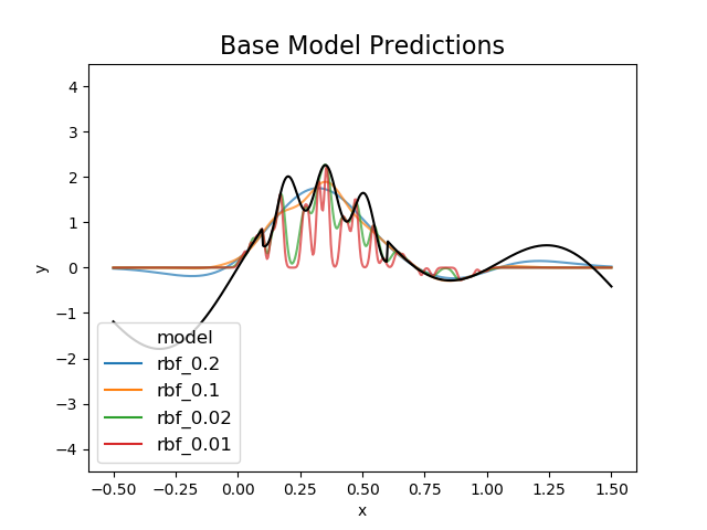
Figure 2: Data generation function and the deterministic predictions from base models in the 1D experiment. Black Line: data-generation function. Colored Line: Base model predictions.

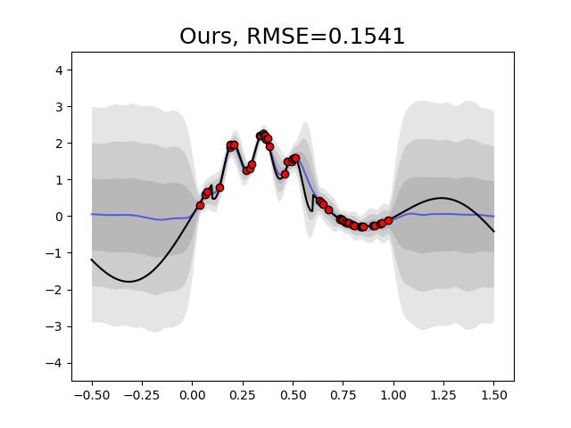
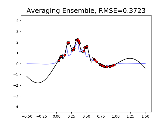
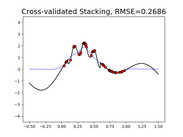
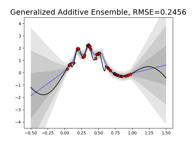
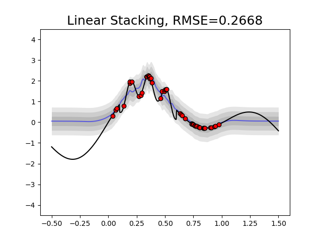
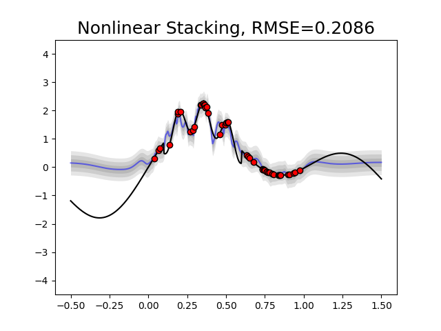
Figure 3: Comparison in prediction and uncertainty quantification of different ensemble methods. The grey bands indicating models’ $68\%$, $95\%$ and $99\%$ predictive interval.

To prepare base models in the ensemble, we randomly generate 20 data points $x_{i}\sim Uniform(0,1)$, and generate $y_{i}=f(x_{i}+\epsilon_{i})$, where $\epsilon_{i}\stackrel{{\scriptstyle i.i.d.}}{{\sim}}N(0,0.01)$ and the data-generating function $f(x)=f_{\mbox{\tiny\tt slow}}(x)+f_{\mbox{\tiny\tt fast}}(x)$ is the composition of a smooth, slow-varying global function $f_{\mbox{\tiny\tt slow}}(x)=x+sin(4*x)+sin(13*x)$ on $x\in(-0.5,1.5)$, and a fast-varying, local function $f_{\mbox{\tiny\tt fast}}(x)=0.5*sin(40*x)$ on $x\in(0.1,0.6)$ (black lines in Figure 3). We train four different kernel regression models on separetely generated datasets, using Radial Basis Function (RBF) kernel with two groups of length-scale parameters ${\tt smooth}=\{0.2,0.1\}$ and ${\tt complex}=\{0.02,0.01\}$ to represent two groups of models with different smoothness assumptions, resulting in $\Fsc=\{\hat{f}_{k}\}_{k=1}^{4}$. As shown in Figure 2, no base model can predict the ground truth universally well across $x\in(0,1)$. We then train all the ensemble methods on a holdout dataset of 20 data points generated using the same mechanism. For our model, we use RBF kernel for both $\bmu$ and $\bepsilon$, where we put prior $LogNormal(-1.,1.)$ on the RBF’s length-scale parameters so they are estimated automatically through the inference procedure. The spline hyperparameters for nlr-stack and gam are selected using random grid search over $10^{3}$ candidates based on model’s cross-validation error.

After training, we evaluate each model’s RMSE on a validation dataset of 500 data points spaced evenly between $x\in(0,1)$. We repeat above training and evaluation procedure 100 times on randomly generated holdout datasets, and report the mean and standard deviation of the validation RMSE in Table 1. We also visualize the models’ behavior in prediction of one such training-evaluation instance in Figure 3.

Performance in Prediction and in Uncertainty Quatification

As shown, comparing the mean prediction (blue line), avg, cv-stack and lnr-stack produce either overly complex or overly smooth fits, due to assigning constant weights to the base models. On the other hand, nlr-stack and gam produce closer fit to the data-generation mechanism. But they tend to overfit the observations in the holdout dataset, producing either unnecessary local fluctuations (nlr-stack), or extrapolating improperly in regions outside $x\in(0,1)$ (gam), resulting in higher validation RMSE compared to that of our model. In comparison, our model produces smooth fit that closely matches the data-generation mechanism where holdout observation is available or the model agreement is high, and produces smooth interpolation with high uncertainty in regions with few holdout observations and model agreement is low (e.g. $x\in(0.5,0.75)$), indicating proper quantification of uncertainty. Examining the predictive intervals of other ensemble methods, we find that these intervals tend to vary less flexibly within the range of $x\in(0,1)$, sometimes failing to reflect the increased uncertainty in regions where the data is sparse and the model agreement is low, and resulting in overly narrow confidence intervals (e.g. gam in $x\in(0.5,0.75)$).

We also quantitatively assessed gam, lnr-stack, nlr-stack and our model’s quality in uncertainty quantification (in terms of the true coverage probability of the $p\%$ predictive intervals for $p\in(0,1]$). In order to assess the effect of the calibrated inference on the model quality in uncertainty quatification, we compare two versions of our model estimated with nd without the CvM distance in inference objective. The result is visualized in Figure A.1, where the x-axis is the nomial coverage probability of model’s predictive interval (in percentage), and the y-axis is the actual coverage probability of model’s predictive interval. Ideally, the coverage curve should align with the black line. For a given coverage percentage, curve below black line indicates underestimated uncertainty (i.e. overly narrow predictive interval), and curve above the black line indicates over-estimated uncertainty (i.e. unnecessarily wide predictive interval). Compared to other ensemble methods, the nominal coverage of our model’s predictive intervals are shown to be closer to their true coverage, and visible improvement can be observed for the model estimated with the CvM distance included in the inference objective.

5 Application: Spatial integration of air pollution predictions in Eastern Massachusetts

In air pollution exposure assessment, many research groups are developing distinct spatio-temporal models (exposure models) to predict ambient air pollution exposures of study participants even in areas where air pollution monitors are sparse. Depending on the prediction model and the inputs, model predictions from different models differ across space and time (Figure 4). However, information on prediction uncertainty is generally unavailable, leading to difficulties in exposure assessment for downstream health effect investigations. Here we use our ensemble method to aggregate the spatio-temporal predictions of three state-of-the-art PM_2.5 exposure models ((Kloog et al., 2014; Di et al., 2016; van Donkelaar et al., 2015) in Figure 4) to produce a single set of spatio-temporal exposure estimates, along with information on predictive uncertainty for these estimates, in Eastern Massachusetts. We implement our ensemble framework on the base models’ out-of-sample prediction for 43 monitors across the greater Boston area for 2011. We used RBF kernels for the ensemble weights $\bmu$, and the Ornstein–Uhlenbeck process kernel for the residual process, following standard practice in spatial modelling literature (Wispelaere, 1984). The length-scale parameters for both kernels are selected through the empirical Bayes procedure. Table 2 reports the leave-one-out RMSE for each of the competing ensemble approaches considered in the simulation study (Section 4), and Figure 5 visualizes the model’s posterior predictions and uncertainty estimates (posterior predictive variance) across the study region, where black circles indicating the locations of the air pollution monitors. As shown, we observed elevated uncertainty southwest of the City of Boston (where the base models disagree) and regions farther away from metropolitan area (where the monitors are sparse), reflecting uncertainty in model combination and in prediction that is consistent with the empirical evidence (also see Figure A.3).

6 Conclusion

In this work, we have presented a principled Bayesian nonparametric approach for combining deterministic model predictions to achieve both spatiotemporally adaptive aggregation, and calibrated uncertainty quantification. Acknowledging challenges in the setting of spatiotemporal prediction for environmental exposures, we took an hypothetico-deductive approach (Gelman and Shalizi, 2013) toward Bayesian modeling. Specifically, we constructed a fully nonparametric model that is flexible both in its systematic component and in its random components, with the systematic component being adaptive in space and time and adopting clear decomposition in different sources of model uncertainty, and the random component being flexible yet respecting proper mathematical constraints. To target the model posterior toward the operating characteristics of interest, we designed a decision-theoretic inference procedure that orients model toward calibration (i.e. consistency between model predictive CDF and the empirical CDF of the data), and proposed an efficient Gibbs algorithm with theoretical guarantee in predictive accuracy. To illustrate the practical effectiveness of our approach, we compared both numerically and visually the performance of our method with that of the classical ensemble methods that are used in machine learning and in environmental modeling, and illustrated clear improvement in both out-of-sample predictive accuracy and in uncertainty quantification. Finally, we applied our method to the real-world task of aggregating air pollution exposure assessment models in greater Boston arae. Our result outperformed that of the previous ensemble approaches in out-of-sample predictive accuracy, and have produced uncertainty quantification in model selection and in prediction that was consistent with empirical evidence.

There are several future directions that we would like to pursue. On the theoretical side, we would like to investigate our model’s behavior in posterior concentration in the Bernstein-von Mises sense (Szabó et al., 2015), and study how such behavior is impacted by the choices of the kernel family and the inference algorithm, and whether the contraction rate is improved by the calibration procedure. On the modeling side, we would like to extend our model to incorporate additional land-use features into the ensemble weights and the residual process, and to model the multivariate outcome of air pollution mixture by aggregating single-exposure models for different pollutant outcomes. On the inference side, we would like to study how to extend our divergence-based inference procedure for additional calibration criteria, such as requiring the spatiotemporal prediction to be sufficiently accurate simultaneously on multiple time scales (e.g. daily, monthly, etc). Finally, on the application side, we would like to extend our method to aggregate air pollution exposure models on the national scale, and study through an counterfactual lense how to use the model’s posterior uncertainty to inform environmental policy makers in the optimal placement air pollution monitors.

Tables and Figures

Model	Ours	avg	cv-stack
Validation RMSE	$0.1531\pm 0.017$	$0.3723\pm 0.028$	$0.2686\pm 0.014$
Model	gam	lnr-stack	nlr-stack
Validation RMSE	$0.2463\pm 0.018$	$0.2623\pm 0.011$	$0.2086\pm 0.012$

Table 1: Mean and Standard Deviation for validation RMSE in 1-D regression task
avg: Averaging Ensemble. cv-stack: Cross-validated Stacking.
gam: Generalized Additive Ensemble. lnr-stack: Linear Stacking. nlr-stack: Nonlinear Stacking.

Model	Ours	avg	cv-stack
loo RMSE	$0.7580\pm 0.0883$	$1.6768\pm 0.124$	$1.5437\pm 0.1275$
Model	gam	lnr-stack	nlr-stack
loo RMSE	$1.0771\pm 0.1566$	$1.1626\pm 0.1421$	$1.2327\pm 0.1265$

Table 2: Mean and Standard Deviation for leave-one-out RMSE for annual $PM_{2.5}$ prediction.
avg: Averaging Ensemble. cv-stack: Cross-validated Stacking.
gam: Generalized Additive Ensemble. lnr-stack: Linear Stacking. nlr-stack: Nonlinear Stacking.

Figure 1: Graphical representation of the proposed model.

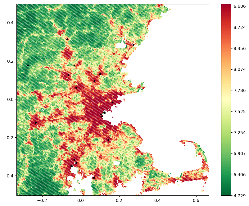
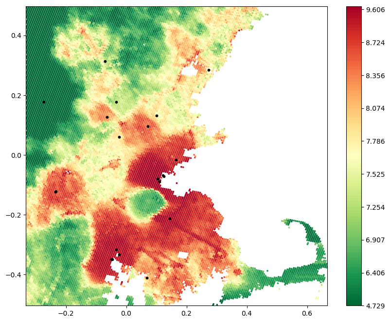
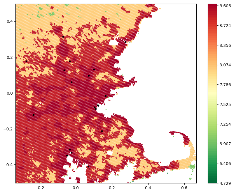
Figure 4: Visualization of annual average PM 2.5 predictions from base air pollution models from greater Boston area in year 2011. (Left) (Kloog et al., 2014); (Middle) (Di et al., 2016); (Right) van Donkelaar et al. (2015)

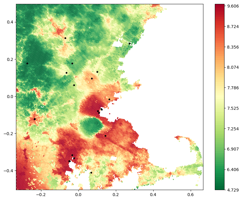
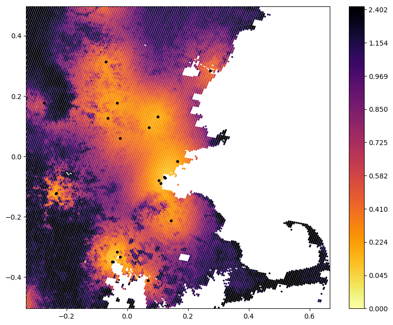
Figure 5: Posterior predictive mean (left) and uncertainty (standard deviation) (right) for annual $PM_{2.5}$ in greater Boston area during year 2011. All unit in $\mu g/m^{3}$. Black Dots: Locations of the air pollution monitors.

Appendix A Additional Figures

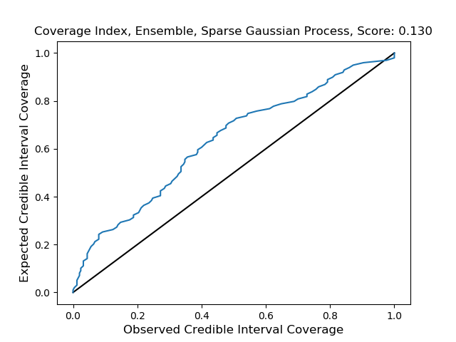
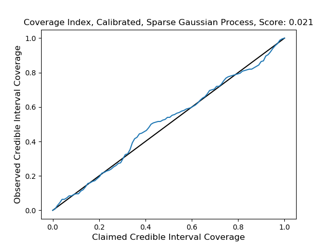
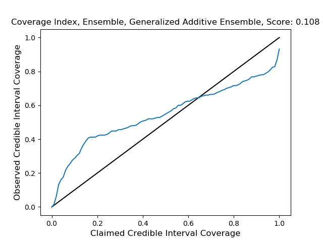
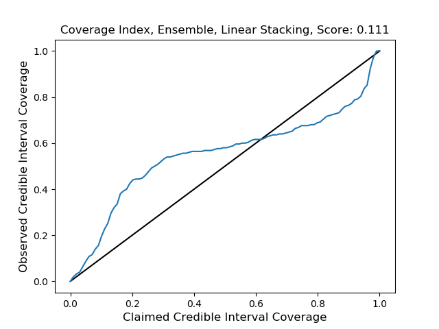
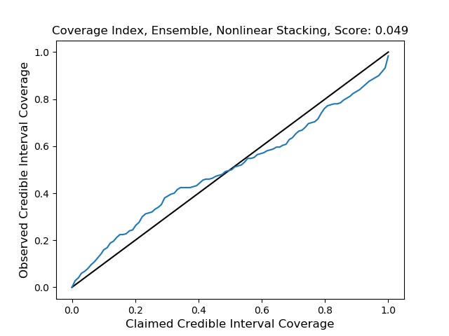
Figure A.1: Comparison in coverage probability of model’s predictive interval of different ensemble methods.
Top Left: Our model, with KL-only VI objective, Top Right Our model with KL+CvM VI objective. Bottom: (from left to right) gam, lnr-stacking and nlr-stacking.

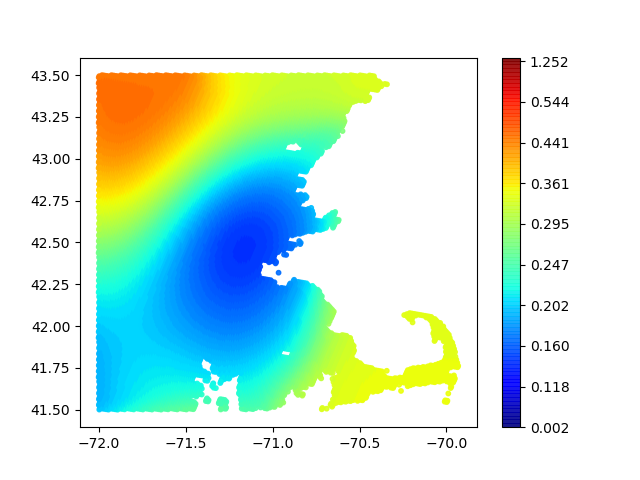
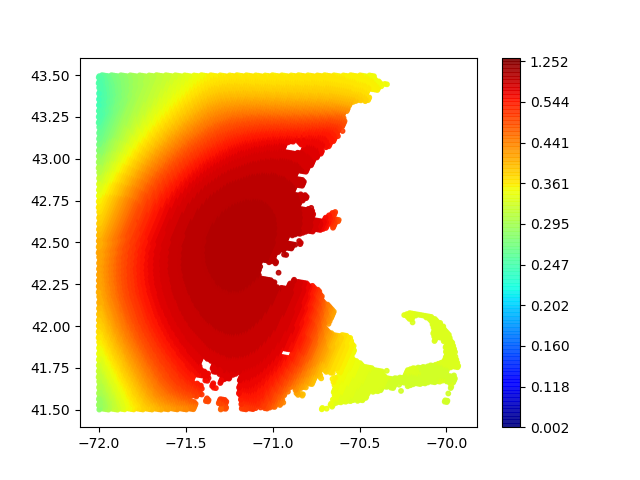
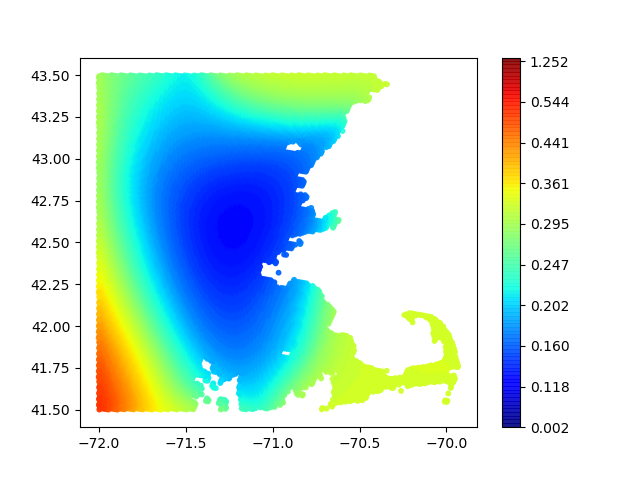
Figure A.2: Adaptive ensemble weight. (Top) Base model predictions and (Bottom) the posterior mean of the ensemble weight Gaussian Process corresponding to each model.

(a) Overall Uncertainty

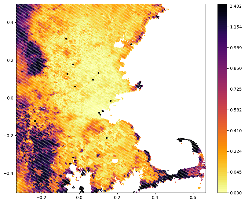
(b) Ensemble Uncertainty

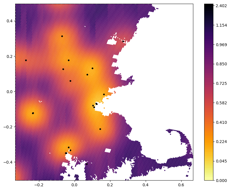
(c) Prediction Uncertainty

Figure A.3: Uncertainty decomposition. Posterior predictive uncertainties (variance) in the full model, the original ensemble model, and the residual process.

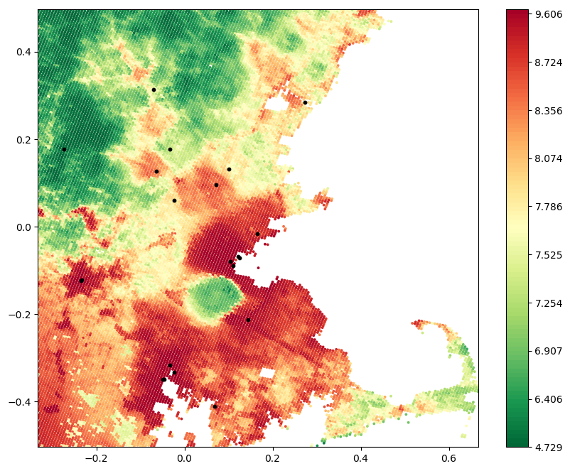
(a) Posterior Mean, Original Ensemble

(b) Posterior Mean, Full Model

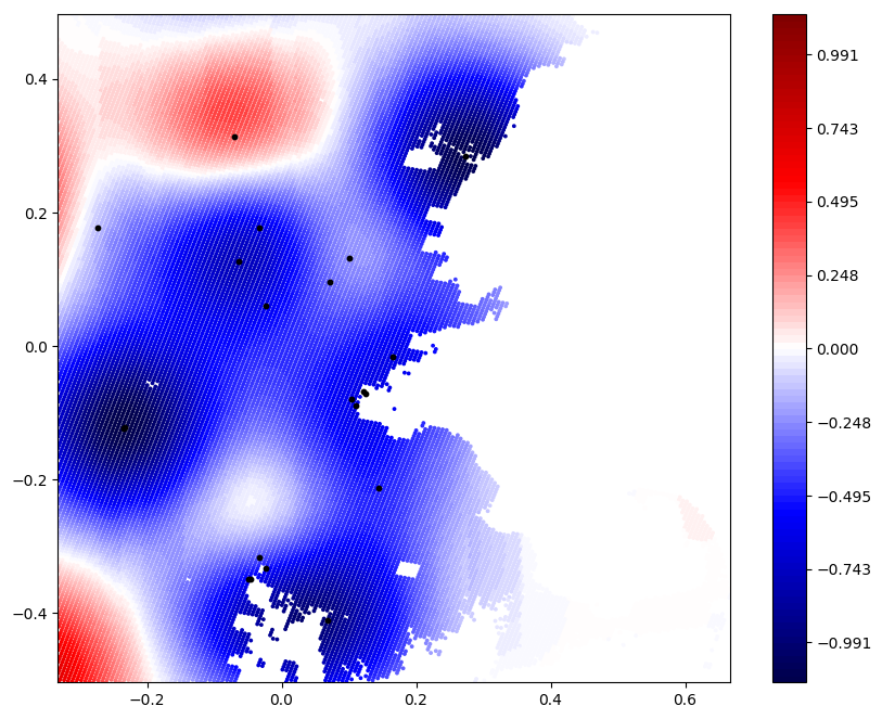
(c) Posterior Mean, Residual Process

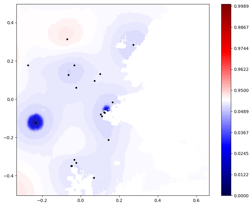
(d) Posterior Confidence in Systematic Bias

Figure A.4: Effect of residual process on model prediction and uncertainty quantification.
First Row: (a)-(b) Posterior predictive mean in the original ensemble (without residual process), and in the full model (with residual process); Second Row: (c) Posterior mean in the residual process, and (d) residual process’s posterior confidence in the systematic bias in original ensemble, i.e. $P(|D_{\delta}(y|\bx)|>0)$

Appendix B Proof for Theorem 3.1

Proof.

For $Y,\bX\sim\Fbb(Y,\bX)$, denote $l(Y,F)(t)=L(Y,F(t|\bX))$ the accuracy measure that involves the observation $Y$ and the corresponding predictive CDF $F(Y|\bX)$ evaluated at $t\in\Ysc$. For an observed data pair $\{y_{i},\bx_{i}\}$, denote the corresponding empirical version of $l$ as $l_{i}(Y,F)(t)=L(y_{i},F(t|\bx_{i}))$. Also denote $F_{i}(t)=F(t|\bX=\bx_{i})$.

We notice below facts:

1. $l(Y,F)(t)$ is bounded by $B$, therefore for any predictive CDFs $F,F^{\prime}\in\Fsc$, we always have:

   $$l(Y,F)(t)-l_{i}(Y,F^{\prime})(t)\leq B$$

2. Since $l(Y,F)(t)$ is proper in the sense that this loss is minimized by the true model parameters, then for $Y\sim\Fbb$:

   $$\Fbb(t)\in\underset{F\in\Fsc}{argmin}\;E_{Y\sim\Fbb}\Big{(}l(Y,F)(t)\Big{)}$$

3. $\bbI\Big{(}\hat{F}_{i}(t)=p_{i}\Big{)}=\bbI\Big{(}\hat{F}_{i}(t)=p_{i},y_{i}<t\Big{)}+\bbI\Big{(}\hat{F}_{i}(t)=p_{i},y_{i}>t\Big{)}$.
   Furthermore,

   $$\bbI\Big{(}\hat{F}_{i}(t)=p_{i},y_{i}<t\Big{)} =\bbI\Big{(}\hat{F}_{i}(t)=p_{i}\Big{)}*\Big{(}\bbI\big{(}y_{i}<t|\hat{F}_{i}(t)=p_{i}\big{)}-p_{i}\Big{)}+\bbI\Big{(}\hat{F}_{i}(t)=p_{i}\Big{)}*p_{i}$$

   $$\bbI\Big{(}\hat{F}_{i}(t)=p_{i},y_{i}>t\Big{)} =\bbI\Big{(}\hat{F}_{i}(t)=p_{i}\Big{)}*\Big{(}p_{i}-\bbI\big{(}y_{i}<t|\hat{F}_{i}(t)=p_{i}\big{)}\Big{)}+\bbI\Big{(}\hat{F}_{i}(t)=p_{i}\Big{)}*\Big{(}1-p_{i}\Big{)}$$

   which implies:

   $$\bbI\Big{(}\hat{F}_{i}(t)=p_{i}\Big{)}\leq 2*\bbI\Big{(}\hat{F}_{i}(t)=p_{i}\Big{)}*\Big{|}\bbI\big{(}y_{i}<t|\hat{F}_{i}(t)=p_{i}\big{)}-p\Big{|}+\bbI\Big{(}\hat{F}_{i}(t)=p_{i}\Big{)}*p_{i}(t)$$

   where $p_{i}(t)=p_{i}$ if $y_{i}<t$ and $p_{i}(t)=1-p_{i}$ otherwise.

Combining above facts, we have:

$$\bbL(Y,\hat{F})(t)-\bbL(Y,\hat{F}_{0})(t) =\frac{1}{N}\sum_{i=1}^{N}\Big{(}l_{i}(Y,\hat{F})(t)-l_{i}(Y,\hat{F}_{0})(t)\Big{)}*\bbI(\hat{F}_{i}(t)=p_{i})$$

$$\leq 2\frac{1}{N}\sum_{i=1}^{N}\underline{\Big{(}l_{i}(Y,\hat{F})(t)-l_{i}(Y,\hat{F}_{0})(t)\Big{)}}*\Big{|}\bbI\big{(}y_{i}<t|\hat{F}_{i}(t)=p_{i}\big{)}-p_{i}\Big{|}*\bbI(\hat{F}_{i}(t)=p_{i})+$$

$$\qquad\frac{1}{N}\sum_{i=1}^{N}\Big{(}l_{i}(Y,\hat{F})(t)-l_{i}(Y,\hat{F}_{0})(t)\Big{)}*p_{i}(t)*\bbI(\hat{F}_{i}(t)=p_{i})$$

$$\leq 2B*\bigg{\{}\frac{1}{N}\sum_{i=1}^{N}\Big{|}\bbI\big{(}y_{i}<t|\hat{F}_{i}(t)=p_{i}\big{)}-p_{i}\Big{|}*\bbI(\hat{F}_{i}(t)=p_{i})\bigg{\}}\;+$$

$$\qquad\bigg{\{}\frac{1}{N}\sum_{i=1}^{N}\Big{(}l_{i}(Y,\hat{F})(t)-l_{i}(Y,\hat{F}_{0})(t)\Big{)}*p_{i}(t)*\bbI(\hat{F}_{i}(t)=p_{i})\bigg{\}}$$ (12)

Here the first inequality uses Fact 3. The second inequality uses Fact 1 on the underlined component.

We now consider the two expressions in curly brackets in (12). Notice the first expression corresponds to an "unintegrated" version of calibration loss:

$$\frac{1}{N}\sum_{i=1}^{N}\Big{|}\bbI\big{(}y_{i}<t|\hat{F}_{i}(t)=p_{i}\big{)}-p_{i}\Big{|}*\bbI(\hat{F}_{i}(t)=p_{i}) =\frac{1}{N}\sum_{i=1}^{N}\Big{|}\bbI\big{(}y_{i}<t|\bx_{i}\big{)}-\hat{F}_{i}(t)\Big{|}=\bbC(Y,\hat{F})(t),$$ (13)

and the second expression can be written as:

$$\quad\frac{1}{N}\sum_{i=1}^{N}\Big{(}l_{i}(Y,\hat{F})(t)-l_{i}(Y,\hat{F}_{0})(t)\Big{)}*p_{i}(t)*\bbI(\hat{F}_{i}(t)=p_{i})$$

$$=\frac{1}{N}\bigg{[}\sum_{y_{i}<t}\Big{(}l_{i}(Y,\hat{F})(t)-l_{i}(Y,\hat{F}_{0})(t)\Big{)}*\hat{F}_{i}(t)+\sum_{y_{i}\geq t}\Big{(}l_{i}(Y,\hat{F})(t)-l_{i}(Y,\hat{F}_{0})(t)\Big{)}*(1-\hat{F}_{i}(t))\bigg{]}$$

$$\leq\frac{1}{N}\bigg{[}\sum_{y_{i}<t}\Big{(}l_{i}(Y,\hat{F})(t)-l_{i}(Y,\hat{F}_{0})(t)\Big{)}*\bbI\big{(}y_{i}<t|\bx_{i}\big{)}+\sum_{y_{i}\geq t}\Big{(}l_{i}(Y,\hat{F})(t)-l_{i}(Y,\hat{F}_{0})(t)\Big{)}*\bbI\big{(}y_{i}>t|\bx_{i}\big{)}\bigg{]}+\epsilon_{n}$$

$$=\mathbb{E}\Big{(}l(Y,\hat{F})(t)-l(Y,\hat{F}_{0})(t)\Big{)}+\epsilon_{n}$$

$$\leq\mathbb{E}\Big{(}l(Y,\Fbb)(t)-l(Y,\hat{F}_{0})(t)\Big{)}+(B+1)\epsilon_{n}$$

$$\leq(B+1)\epsilon_{n}$$ (14)

where the first inequality follows since $\hat{F}$ is $\epsilon_{n}$-calibrated, the second inequality follows since $l$ is a bounded loss, and the last inequality follows since $l$ is a proper loss.

Now replace the two expressions within brackets in (12) with (13) and (14), we have:

$$\bbL(Y,\hat{F})(t)-\bbL(Y,\hat{F}_{0})(t) \leq 2B*\bbC(Y,\hat{F})(t)+(B+1)\epsilon_{n}$$

Intergrating both sides of above equation with respect to $t\in\Ysc$, we have:

$$\bbL(Y,\hat{F})-\bbL(Y,\hat{F}_{0})\leq 2B*\bbC(Y,\hat{F})+(B+1)\epsilon_{n}$$

∎

Appendix C Variational Inference

In general, Variational inference (VI) scales up Bayesian inference by casting posterior estimation as an optimization problem. Briefly, denoting $\btheta$ as the collection of model parameters, VI aim to approximate the target posterior $P(\bz|\{\bx_{i},y_{i}\})$ using a variational distribution $Q_{\btheta}(\bz)$ by minimizing the distance between $P$ and $Q$ with respect to certain variational inference objective $\Lsc(P,Q_{\btheta}|\{\bx_{i},y_{i}\})$ with respect to the variational parameters $\btheta$. However, since in (3) our target divergence of interest is a general divergence measure, the standard expression for the varitional inference objective known as the evidence lower bound (ELBO) (Blei et al., 2016) no longer applies since it is designed for KL divergence. Consequently, in the next two subsections, we first derive the objective function for the variational inference with respect to the general divergence measure $\hat{l}$ in (3) from the first principle, and then discuss suitable choices for the variational family $Q_{\btheta}(\bz)$ in order to achieve accurate quantification of posterior uncertainty.

C.1 Variational Objective for General Divergence

Recall that the posterior update rule for a general divergence measure is written as:

$$P(\bz|\{\bx_{i},y_{i}\}) \propto exp\Big{(}-\hat{l}(y_{i}|\bx_{i},\bz)\Big{)}P(\bz),$$

and the goal of variational inference is to find $Q_{\btheta}(\bz)$ that is closest to the $P(\bz|\{y_{i},\bx_{i}\})$ in terms of the KL divergence:

$$KL\Big{(}Q_{\btheta}(\bz),P(\bz|\{\bx_{i},y_{i}\})\Big{)} =E\Big{(}log\,Q_{\btheta}(\bz)\Big{)}-E\Big{(}log\,P(\bz|\{\bx_{i},y_{i}\})\Big{)}$$

$$=E\Big{(}log\,Q_{\btheta}(\bz)\Big{)}+E\Big{(}\hat{l}(y_{i}|\bx_{i},\bz)\Big{)}-E\Big{(}log\,P(\bz)\Big{)}+C,$$

$$=E\Big{(}\hat{l}(y_{i}|\bx_{i},\bz)\Big{)}+KL\Big{(}Q_{\btheta}(\bz),P(\bz)\Big{)}+C$$

where all expectations are taken over $Q_{\btheta}(\bz)$, and $C=\int_{\bz}exp\Big{(}-\hat{l}(y_{i}|\bx_{i},\bz)\Big{)}P(\bz)d\bz$ is a positive constant term that does not depend on $\bz$. Consequently, we can minimize $KL\Big{(}Q_{\btheta}(\bz),P(\bz|\{\bx_{i},y_{i}\})\Big{)}$ by minimizing below objective function:

$$\Lsc(P,Q_{\btheta}|\{\bx_{i},y_{i}\}) =E\Big{(}\hat{l}(y_{i}|\bx_{i},\bz)\Big{)}+KL\Big{(}Q_{\btheta}(\bz),P(\bz)\Big{)},$$

i.e. the evidence lower bound (ELBO) (Blei et al., 2016) for general divergence measure $\hat{l}(y_{i}|\bx_{i},\bz)$.

To obtain the expression of $\Lsc(P,Q_{\btheta}|\{\bx_{i},y_{i}\})$ for our model, we denote $\bz=\{\bTheta,G\}$ and plug in the expression of $\hat{l}(y_{i}|\bx_{i},\bz)$ from (4):

$$\Lsc(P,Q_{\btheta}|\{\bx_{i},y_{i}\})= E\Big{(}-log\,f(y_{i}|\bx_{i},\bz)\Big{)}+\frac{1}{M}\sum_{j=1}^{M}E\Big{(}\big{[}F(y_{j}|\bx_{i},\bz)-\Ibb(y_{i}<y_{j}|\bx_{i})\big{]}^{2}\Big{)}+$$ (15)

$$KL\Big{(}Q_{\btheta}(\bz),P(\bz)\Big{)},$$ (16)

where all expectations are taken over $Q_{\btheta}(\bz)$. As shown, this inference objective is structured as a regularized loss that orients the variational distribution $Q_{\btheta}(\bz)$ toward both model goodness-of-fit (the first term) and calibration (the second term), while at the same time constraints the $Q_{\btheta}(\bz)$ to be not too far from model prior $P(\bz)$ (the third term). Finally, estimation proceeds by minimizing above inference objective with respect to the variational parameter $\btheta$ using gradient descent, i.e.

$$\btheta^{*} =\underset{\btheta}{argmin}\quad\Lsc(P,Q_{\btheta}|\{\bx_{i},y_{i}\}),$$

and the gradient can be computed using the standard score gradient methods (paisley_variational_2012-1).

C.2 Variational Family

Due to our focus on reliable uncertainty quantification, we find the naive mean-field approximation with fully-factored Gaussians tend to under-estimate predictive uncertainty, and produces non-smooth predictions that overfits the observation. Consequently in this work, we consider an structured variational family known as sparse Gaussian process (SGP) (Titsias, 2009). Specifically, we factor the variational family into independent groups of Gaussian processes $\{\bepsilon,\Gsc\}$ and variance/temperature parameters $\{\sigma,\lambda\}$ as

$$Q_{\btheta}(\bz)=\Big{[}Q_{\btheta_{\epsilon}}(\bepsilon)*\prod_{g\in\Gsc}Q_{\btheta_{g}}(g)\Big{]}*\Big{[}Q_{\btheta_{\sigma}}(\sigma)*Q_{\btheta_{\lambda}}(\lambda)\Big{]},$$

where we model $q(\sigma)$ and $q(\lambda)$’s using fully factored log normal distributions, and model $q(\bepsilon)$ and $q(g)$’s using the SGP, i.e. for a Gaussian process $\bG$ evaluated over $N$ data points $\bX=\{\bx_{i}\}_{i=1}^{N}$, we assume it is stochastically dependent on a smaller (or sparser) Gaussian process $\bG_{0}$ evaluated at a smaller set of $M$ inducing points $\bZ=\{\bz_{j}\}_{j=1}^{M}$ such that

$$P(\bG,\bG_{0})=P(\bG|\bG_{0})P(\bG_{0}).$$

In sparse Gaussian process, the variational family $Q_{\btheta_{G}}(\bG,\bG_{0})$ for this joint distribution $P(\bG,\bG_{0})$ is

$$Q_{\btheta_{G}}(\bG,\bG_{0})=P(\bG|\bG_{0})Q_{\btheta_{G}}(\bG_{0}),\qquad\mbox{where}\qquad Q_{\btheta_{G}}(\bG_{0})=N(\bm,\bS),$$

with variational parameters $\btheta_{G}=\{\bm_{M\times 1},\bS_{M\times M}\}$. Consequently, the variational family $Q_{\btheta_{G}}(\bG)$ for $P(\bG)$ can be obtained in closed form by marginalizing out $\bG_{0}$. Specifically, since $\bG,\bG_{0}$ conditional on observations are jointly Gaussian, the marginalized expression for $Q_{\btheta_{G}}(\bG)$ adopts a closed form (Rasmussen and Williams, 2006):

$$Q_{\btheta_{G}}(\bG) =N(\bG|\bmu,\bSigma)$$ (17)

$$\bmu =\bK_{\bX\bZ}\bK_{\bZ\bZ}^{-1}\bm$$

$$\bSigma =\bK_{\bX\bX}-\bK_{\bX\bZ}\bK_{\bZ\bZ}^{-1}(\bK_{\bZ\bZ}-\bS)\bK_{\bZ\bZ}^{-1}\bK_{\bX\bZ}^{T}.$$

The computation complexity for sparse Gaussian process is $O(NM+M^{3})$ for $N$ data points and $M$ inducing points. Here the expensive cubic complexity $M^{3}$ is caused by the need of inverting the $M\times M$ matrix $\bK_{\bZ\bZ}$. Consequently, the choice of the number of inducing points results in a trade-off between inference quality and computation complexity, as the increased number of inducing points will result in better approximation of the Gaussian process posterior, but at the same time cause cubic increase in computation time.

To tackle this problem, in our implementation we adopt the de-coupled version of sparse Gaussian process (18) known as de-coupled Gaussian process (DGP) (Cheng and Boots, 2017). Derived by treating Gaussian process as a Gaussian measure with its mean and covariance operator defined using different basis functions, DGP use different inducing points to approximate $\mu$ and $\bSigma$, i.e. select $M_{m}$ inducing points $\bZ_{m}=\{\bz_{m,i}\}_{i=1}^{M_{m}}$ for the variational mean $\bm_{M_{m}\times 1}$, and a separate, smaller set of $M_{S}$ inducing points $\bZ_{S}=\{\bz_{S,i}\}_{i=1}^{M_{S}}$ for the variational covariance $\bS_{M_{S}\times M_{S}}$. Consequently, through suitable simplication, the variational family is reduced to:

$$Q_{\btheta_{G}}(\bG) =N(\bG|\bmu,\bSigma)$$ (18)

$$\bmu =\bK_{\bX\bZ_{m}}\bm,\qquad\bSigma=\bK_{\bX\bX}-\bK_{\bX\bZ_{S}}(\bK_{\bZ_{S}\bZ_{S}}^{-1}+\bS)^{-1}\bK_{\bX\bZ_{S}}^{T}.$$

with the computation complexity reduced to $O(NM_{m}+NM_{S}+M_{S}^{3})$. Therefore one can dramatically improve the model’s approximation quality by increase $M_{m}$ which induces only linear increase in computation complexity.

References

- Abernethy et al. (2011) Abernethy, J., Bartlett, P. L., and Hazan, E. (2011). Blackwell Approachability and No-Regret Learning are Equivalent. In Proceedings of the 24th Annual Conference on Learning Theory, pages 27–46.
- Basu et al. (2011) Basu, A., Shioya, H., Park, C., Shioya, H., and Park, C. (2011). Statistical Inference : The Minimum Distance Approach. Chapman and Hall/CRC.
- Bissiri et al. (2016) Bissiri, P. G., Holmes, C. C., and Walker, S. G. (2016). A general framework for updating belief distributions. Journal of the Royal Statistical Society: Series B (Statistical Methodology) 78, 1103–1130.
- Blei et al. (2016) Blei, D. M., Kucukelbir, A., and McAuliffe, J. D. (2016). Variational Inference: A Review for Statisticians. arXiv:1601.00670 [cs, stat] arXiv: 1601.00670.
- Breiman (1996) Breiman, L. (1996). Stacked regressions. Machine Learning 24, 49–64.
- Carlin et al. (2000) Carlin, B. P., Louis, T. A., and Carlin, B. (2000). Bayes and Empirical Bayes Methods for Data Analysis, Second Edition. Chapman and Hall/CRC, Boca Raton, 2 edition edition.
- Cesa-Bianchi and Lugosi (2006) Cesa-Bianchi, N. and Lugosi, G. (2006). Prediction, Learning, and Games. Cambridge University Press, Cambridge ; New York.
- Cheng and Boots (2017) Cheng, C.-A. and Boots, B. (2017). Variational Inference for Gaussian Process Models with Linear Complexity. In Guyon, I., Luxburg, U. V., Bengio, S., Wallach, H., Fergus, R., Vishwanathan, S., and Garnett, R., editors, Advances in Neural Information Processing Systems 30, pages 5184–5194. Curran Associates, Inc.
- Clydec and Iversen (2013) Clydec, M. and Iversen, E. S. (2013). Bayesian model averaging in the M-open framework. Oxford University Press.
- Di et al. (2016) Di, Q., Koutrakis, P., and Schwartz, J. (2016). A hybrid prediction model for PM2.5 mass and components using a chemical transport model and land use regression. Atmospheric Environment 131, 390–399.
- Donnet et al. (2018) Donnet, S., Rivoirard, V., Rousseau, J., and Scricciolo, C. (2018). Posterior concentration rates for empirical Bayes procedures with applications to Dirichlet process mixtures. Bernoulli 24, 231–256.
- Gelman and Shalizi (2013) Gelman, A. and Shalizi, C. R. (2013). Philosophy and the practice of Bayesian statistics. British Journal of Mathematical and Statistical Psychology 66, 8–38.
- Ghosh and Basu (2016) Ghosh, A. and Basu, A. (2016). Robust Bayes estimation using the density power divergence. Annals of the Institute of Statistical Mathematics 68, 413–437.
- Gneiting et al. (2007) Gneiting, T., Balabdaoui, F., and Raftery, A. E. (2007). Probabilistic forecasts, calibration and sharpness. Journal of the Royal Statistical Society: Series B (Statistical Methodology) 69, 243–268.
- Gneiting and Raftery (2007) Gneiting, T. and Raftery, A. E. (2007). Strictly Proper Scoring Rules, Prediction, and Estimation. Journal of the American Statistical Association 102, 359–378.
- Hoeting et al. (1999) Hoeting, J. A., Madigan, D., Raftery, A. E., and Volinsky, C. T. (1999). Bayesian model averaging: a tutorial (with comments by M. Clyde, David Draper and E. I. George, and a rejoinder by the authors. Statistical Science 14, 382–417.
- Jara and Hanson (2011) Jara, A. and Hanson, T. E. (2011). A class of mixtures of dependent tail-free processes. Biometrika 98, 553–566.
- Jewson et al. (2018) Jewson, J., Smith, J. Q., and Holmes, C. (2018). Principles of Bayesian Inference using General Divergence Criteria. Entropy 20, 442. arXiv: 1802.09411.
- Kiureghian and Ditlevsen (2009) Kiureghian, A. D. and Ditlevsen, O. (2009). Aleatory or epistemic? Does it matter? Structural Safety 31, 105–112.
- Kloog et al. (2014) Kloog, I., Chudnovsky, A. A., Just, A. C., Nordio, F., Koutrakis, P., Coull, B. A., Lyapustin, A., Wang, Y., and Schwartz, J. (2014). A new hybrid spatio-temporal model for estimating daily multi-year PM2.5 concentrations across northeastern USA using high resolution aerosol optical depth data. Atmospheric Environment 95, 581–590.
- Kuleshov and Ermon (2017) Kuleshov, V. and Ermon, S. (2017). Estimating Uncertainty Online Against an Adversary. In Proceedings of the Thirty-first AAAI Conference on Artificial Intelligence.
- Kull et al. (2017) Kull, M., Filho, T. S., and Flach, P. (2017). Beta calibration: a well-founded and easily implemented improvement on logistic calibration for binary classifiers. In Artificial Intelligence and Statistics, pages 623–631.
- Lorenzi and Filippone (2018) Lorenzi, M. and Filippone, M. (2018). Constraining the Dynamics of Deep Probabilistic Models. arXiv:1802.05680 [stat] arXiv: 1802.05680.
- Millar (1981) Millar, P. W. (1981). Robust estimation via minimum distance methods. Zeitschrift für Wahrscheinlichkeitstheorie und Verwandte Gebiete 55, 73–89.
- Nakagawa and Hashimoto (2018) Nakagawa, T. and Hashimoto, S. (2018). Robust Bayesian inference via Gamma Divergence. Communications in Statistics - Theory and Methods page 19.
- Neal (2012) Neal, R. M. (2012). MCMC using Hamiltonian dynamics. arXiv:1206.1901 [physics, stat] arXiv: 1206.1901.
- Raftery et al. (2005) Raftery, A. E., Gneiting, T., Balabdaoui, F., and Polakowski, M. (2005). Using Bayesian Model Averaging to Calibrate Forecast Ensembles. Monthly Weather Review 133, 1155–1174.
- Raftery et al. (2003) Raftery, A. E., Zheng, Y., We, N., Clyde, M., Hoeting, J., and Madigan, D. (2003). Long Run Performance of Bayesian Model Averaging.
- Rasmussen and Williams (2006) Rasmussen, C. E. and Williams, C. K. I. (2006). Gaussian Processes for Machine Learning. University Press Group Limited. Google-Books-ID: vWtwQgAACAAJ.
- Riihimäki and Vehtari (2010) Riihimäki, J. and Vehtari, A. (2010). Gaussian processes with monotonicity information. In Proceedings of the Thirteenth International Conference on Artificial Intelligence and Statistics, pages 645–652.
- Selten (1998) Selten, R. (1998). Axiomatic Characterization of the Quadratic Scoring Rule. Experimental Economics 1, 43–61.
- Smola et al. (2000) Smola, A. J., Bartlett, P. J., Schuurmans, D., and Schölkopf, B. (2000). Advances in Large Margin Classifiers. MIT Press. Google-Books-ID: gOXI3fO3VUwC.
- Sniekers and Vaart (2015) Sniekers, S. and Vaart, A. v. d. (2015). Adaptive Bayesian credible sets in regression with a Gaussian process prior. Electronic Journal of Statistics 9, 2475–2527.
- Szabó et al. (2015) Szabó, B., van der Vaart, A. W., and van Zanten, J. H. (2015). Frequentist coverage of adaptive nonparametric Bayesian credible sets. The Annals of Statistics 43, 1391–1428. arXiv: 1310.4489.
- Thomas et al. (2007) Thomas, D. C., Jerrett, M., Kuenzli, N., Louis, T. A., Dominici, F., Zeger, S., Schwarz, J., Burnett, R. T., Krewski, D., and Bates, D. (2007). Bayesian Model Averaging in Time-Series Studies of Air Pollution and Mortality. Journal of Toxicology and Environmental Health, Part A 70, 311–315.
- Titsias (2009) Titsias, M. (2009). Variational Learning of Inducing Variables in Sparse Gaussian Processes. In Artificial Intelligence and Statistics, pages 567–574.
- Vaart and Zanten (2011) Vaart, A. v. d. and Zanten, H. v. (2011). Information Rates of Nonparametric Gaussian Process Methods. Journal of Machine Learning Research 12, 2095–2119.
- Vaart and Zanten (2009) Vaart, A. W. v. d. and Zanten, J. H. v. (2009). Adaptive Bayesian estimation using a Gaussian random field with inverse Gamma bandwidth. The Annals of Statistics 37, 2655–2675.
- van Donkelaar et al. (2015) van Donkelaar, A., Martin, R. V., Spurr, R. J. D., and Burnett, R. T. (2015). High-Resolution Satellite-Derived PM2.5 from Optimal Estimation and Geographically Weighted Regression over North America. Environmental Science & Technology 49, 10482–10491.
- Wahba (1990) Wahba, G. (1990). Spline Models for Observational Data. SIAM. Google-Books-ID: ScRQJEETs0EC.
- Walker (2013) Walker, S. G. (2013). Bayesian inference with misspecified models. Journal of Statistical Planning and Inference 143, 1621–1633.
- Walker et al. (2003) Walker, W. E., Harremoës, P., Rotmans, J., Van der Sluijs, J. P., Van Asselt, M. B. A., Janssen, P., and Krayer von Krauss, M. P. (2003). Defining Uncertainty: A Conceptual Basis for Uncertainty Management in Model-Based Decision Support. Integrated Assessment, 4, 2003 .
- Wispelaere (1984) Wispelaere, C. D. (1984). Air Pollution Modeling and Its Application III. Nato Challenges of Modern Society. Springer US.
- Xiao et al. (2018) Xiao, Q., Chang, H. H., Geng, G., and Liu, Y. (2018). An ensemble machine-learning model to predict historical PM2.5 concentrations in China from satellite data. Environmental Science & Technology .
- Zadrozny and Elkan (2002) Zadrozny, B. and Elkan, C. (2002). Transforming Classifier Scores into Accurate Multiclass Probability Estimates. In Proceedings of the Eighth ACM SIGKDD International Conference on Knowledge Discovery and Data Mining, KDD ’02, pages 694–699, New York, NY, USA. ACM.