On an inverse source problem for the full radiative transfer equation with incomplete data

Abstract

A new numerical method to solve an inverse source problem for the radiative transfer equation involving the absorption and scattering terms, with incomplete data, is proposed. No restrictive assumption on those absorption and scattering coefficients is imposed. The original inverse source problem is reduced to boundary value problem for a system of coupled partial differential equations of the first order. The unknown source function is not a part of this system. Next, we write this system in the fully discrete form of finite differences. That discrete problem is solved via the quasi-reversibility method. We prove the existence and uniqueness of the regularized solution. Especially, we prove the convergence of regularized solutions to the exact one as the noise level in the data tends to zero via a new discrete Carleman estimate. Numerical simulations demonstrate good performance of this method even when the data is highly noisy.

35R30

1 Introduction

The stationary radiative transfer equation (RTE) is commonly used in optics, tomography, astrophysics, atmospheric science and remote sensing to describe the propagation of the radiation field in media with absorbing, emitting and scattering radiation. A significant number of studies is dedicated to the recovery of the parameters of the observed objects from the measured data; i.e., to the solutions of the inverse source problems (ISOPs) [1, 24] and coefficient inverse problems (CIPs) [2, 33]. A number of inverse problems may be formulated, depending on the object’s parameters of one’s interest.

The first reconstruction formula for the problem of the attenuated tomography was obtained by Novikov [31]. We also refer to [3, 12, 29] for reconstruction formulae and as well as to [10, 29] for numerical results for the attenuated tomography with complete data and with the scattering phase function $K\equiv 0$. Uniqueness and stability results for similar ISOPs with complete data were obtained in [3, 34]. It was assumed in [3] that $\left|K\right|$ is sufficiently small. The assumption of [34] is that functions $\sigma$ and $K$ belong to certain dense sets of some function spaces. The scattering phase function $K$ is involved in RTE as the kernel of a certain integral operator, the attenuation coefficient is $\sigma=\mu_{a}+\mu_{s}$, where $\mu_{a}$ and $\mu_{s}$ are the absorption and scattering coefficients respectively, see Section 2.

In this paper, we propose a new numerical approach for the ISOP with limited angle data for the stationary RTE and prove its convergence. This is the first publication, in which a rigorously derived numerical method for the ISOP for the RTE does not use any restrictive assumptions neither on $\mu_{a},$ nor on $\mu_{s},$ nor on $K$, except the smoothness and the requirement that functions $\mu_{a}$ and $\mu_{s}$ are compactly supported. Also, for the first time, a discrete Carleman estimate is applied here for the convergence analysis of an inverse problem. We note that discrete Carleman estimates are very rare, unlike the continuous ones. In addition, we prove the Lipschitz stability and uniqueness for our statement of the ISOP.

Our method is based on the solution of an overdetermined boundary value problem for a linear system of coupled integro-differential equations, in which the unknown source function is not present. The solution of this problem directly yields the solution of the desired ISOP. A similar idea was recently used in [23]. However, unlike the current paper, a quite restrictive condition $\sigma\equiv K\equiv 0$ is imposed in [23]. The ISOP for the RTE with limited angle data has many applications in optical imaging and tomography, such as bioluminescence tomography [13] and X-ray computerized tomography [27, 28].

The idea of our numerical method has roots in the Bukhgeim-Klibanov method (BK) [9]. BK was originally proposed in 1981 only for proofs of global uniqueness and stability results for CIPs for PDEs, rather than for numerical methods. BK is based on Carleman estimates. Since the current paper is not a survey of BK, we refer here only to a few publications about BK [5, 6, 15, 16, 17] and references cited therein. Currently, the idea of BK is extensively used for constructions of globally convergent numerical methods for CIPs for PDEs, see, e.g. [4, 18, 21, 22].

The second important element of our numerical method is the new orthonormal basis in the space $L^{2}\left(a,b\right),\left(a,b\right)\subset\mathbb{R}$, which was recently introduced in [20]. This basis has proven to be effective for numerical studies [21, 22, 23]. We use a truncated Fourier series with respect to this basis. We estimate an optimal number of terms of this series numerically and assume that this approximation still satisfies the RTE, i.e. we work with an approximate mathematical model, also, see Remark 4 at the end of Section 5.

We solve the above mentioned overdetermined boundary value problem by the quasi-reversibility method (QRM), which is known to be effective to solve overdetermined boundary value problems. We consider a fully discrete form of our system, which is similar to what we use in the numerical tests. Next, we establish a new discrete Carleman estimate and use it to prove uniqueness and existence of the regularized solution for the QRM in the fully discrete form, in which partial derivatives with respect to spatial variables are written via finite differences. This Carleman estimate is also used to establish the convergence rate of regularized solutions. Finally, we conduct numerical testing for several different regimes of absorption and scattering to show the method’s potential for solving problems in real-world tomography.

The QRM was originally introduced by Lattes and Lions in 1969 [25]. We also refer to, e.g. [7, 8, 12, 23] for this method. The second author has shown in the survey paper [19] that as long as a proper Carleman estimate for an ill-posed problem for a linear PDE is available, the convergent QRM can be constructed for this problem.

For brevity, we consider in this paper only the 2D case. The considerations in the 3D case are similar. We state both forward and inverse problems in Section 2. In Section 3 we derive the above mentioned over-determined boundary value problem for a system of coupled partial differential equations of the first order. To solve this problem, we apply the QRM by stating a Minimization Problem. In Section 4 we introduce the fully discrete version of the quasi-reversibility method to solve that problem. Next, we derive a new discrete Carleman estimate. This estimate is used in Section 5 to prove the existence and uniqueness of the minimizer of the QRM and also to establish the convergence rate of the minimizers to the exact solution as the level of noise in the measured data tends to zero. Section 6 is devoted to numerical studies. Everywhere below we work only with real-valued functions.

2 Statements of Forward and Inverse Problems

Let $\mathbf{x}=(x,y)$ denote an arbitrary point in $\mathbb{R}^{2}$. Let $a,b,d$ and $R$ be the positive numbers, where $1<a<b$ and $d\geq R$. Define the rectangular domain $\Omega\subset\mathbb{R}^{2}$ (Figure 1) as

(1) $$\Omega=\{(x,y):-R<x<R,a<y<b\}.$$

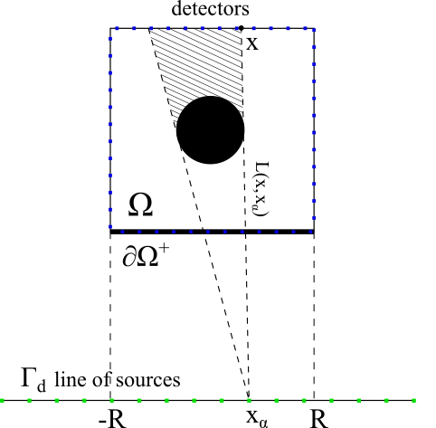
(a) The source/detector configuration of the problem in the case when the source located at $\mathbf{x}_{\alpha}$ with $\left|\mathbf{x}_{\alpha}\right|<R.$

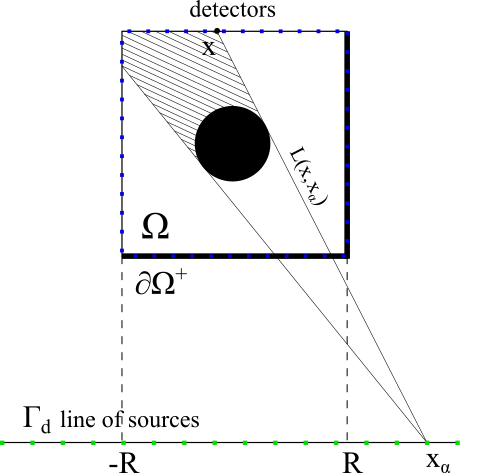
(b) The source/detector configuration of the problem in the case when the source located at $\mathbf{x}_{\alpha}$ with $\left|\mathbf{x}_{\alpha}\right|>R.$

Figure 1: A schematic diagram of measurements for the 2D case. $L(\mathbf{x},\mathbf{x}_{\alpha})$ is a straight line, connecting the detector $\mathbf{x}$ with the source $\mathbf{x}_{\alpha}$.

Let $\Gamma_{d}$ be the line with external sources

(2) $$\Gamma_{d}=\{\mathbf{x}_{\alpha}=(\alpha,0):\alpha\in[-d,d]\}.$$

Let $u(\mathbf{x},\alpha)$ denotes the steady-state radiance at the point $\mathbf{x}$ generated by the external source located at $\mathbf{x}_{\alpha}=(\alpha,0)\in\Gamma_{d}$. Then, the function $u(\mathbf{x},\alpha)$ satisfies the following radiative transfer equation, see, e.g. [11]

(3) $$\nu(\mathbf{x},\alpha)\cdot\nabla_{\mathbf{x}}u(\mathbf{x},\alpha)+(\mu_{a}(\mathbf{x})+\mu_{s}(\mathbf{x}))u(\mathbf{x},\alpha)\\ =\mu_{s}(\mathbf{x})\int_{\Gamma_{d}}K(\mathbf{x},\alpha,\beta)u(\mathbf{x},\beta)d\beta+f(\mathbf{x})\quad\mbox{for all }\mathbf{x}\in\Omega.$$

In the equation above, the function $f(\mathbf{x})\in L^{2}(\mathbb{R}^{2})$ is called the source function while the functions $\mu_{a}(\mathbf{x})$, $\mu_{s}(\mathbf{x})\in C^{1}\left(\mathbb{R}^{2}\right)$ denote the absorption and scattering coefficients respectively. We assume that

(4) $$\mu_{a}(\mathbf{x})=\mu_{s}(\mathbf{x})=f\left(\mathbf{x}\right)=0\quad\mbox{for all }\mathbf{x}\in\mathbb{\mathbb{R}}^{2}\setminus\Omega.$$

The function $K(\mathbf{x},\alpha,\beta)\in C^{1}(\mathbb{R}^{2}\times[-d,d]^{2})$ represents the so-called “scattering phase function”. Scattering phase function is the probability density of a particle scattering from $\nu(\mathbf{x},\beta)$-direction into $\nu(\mathbf{x},\alpha)$-direction. As the probability density, $K(\mathbf{x},\alpha,\beta)$ possesses the following properties, discussed in detail in [11]

(5) $$K(\mathbf{x},\alpha,\beta)\geq 0,\quad\int_{\Gamma_{d}}\int_{\Gamma_{d}}K(\mathbf{x},\alpha,\beta)d\alpha d\beta=1.$$

Finally, $\nu(\mathbf{x},\alpha)$ is the $\mathbb{R}^{2}-$vector, showing the direction of particles propagating from the external source located at $\mathbf{x}_{\alpha}=(\alpha,0)$ to $\mathbf{x,}$

(6) $$\nu(\mathbf{x},\alpha)=\left(\frac{x-\alpha}{|\mathbf{x}-\mathbf{x}_{\alpha}|},\frac{y}{|\mathbf{x}-\mathbf{x}_{\alpha}|}\right),\quad x\in[-R,R],\quad y\in[a,b],\quad\alpha\in[-d,d].$$

For a fixed $\alpha$, let

$$\partial\Omega^{+}=\left\{\mathbf{x}\in\partial\Omega:\nu(\mathbf{x},\alpha)\cdot\mathbf{n}(\mathbf{x})\leq 0\right\},$$

where $\mathbf{n}(\mathbf{x})$ is the unit outward normal vector at $\partial\Omega$ at point $\mathbf{x}$. Assuming that all functions in equation (3), except ${u(\mathbf{x},\alpha)},$ are known in $\Omega$, we formulate the following forward problem.

Problem 2.1 (Forward Problem).

For each $\alpha\in\left[-d,d\right],$ find the function ${u(\mathbf{x},\alpha)},$ satisfying equation (3) in the domain $\Omega$ as well as the following boundary condition

(7) $$u(\mathbf{x},\alpha)=0\quad\mbox{for all }\mathbf{x}\in\partial\Omega^{+}.$$

In Appendix we prove existence and uniqueness of the solution of the boundary value problem (3), (7) and; moreover, discuss a numerical method to solve it. Conversely, assume now that the function $f(\mathbf{x})$ is unknown and the information of $u(\mathbf{x},\alpha)$ on $\partial\Omega$ is known. The main goal of this paper is to numerically solve the following inverse source problem:

Problem 2.2 (Inverse Source Problem).

Assume that equation (3) and conditions (4), (5) hold. Also, let the vector $\nu(\mathbf{x},\alpha)$ in (3) has the form (6). Reconstruct the function $f(\mathbf{x}),$ $\mathbf{x}\in\Omega,$ given the following boundary data

(8) $$F(\mathbf{x},\alpha)=u(\mathbf{x},\alpha),\quad\mbox{for all }\mathbf{x}\in\partial\Omega,\alpha\in[-d,d],$$

where ${u(\mathbf{x},\alpha)}$ is the solution of Problem 7 and

(9) $$F(\mathbf{x},\alpha)=0\text{ }\textit{for}\text{ }\mathbf{x}\in\partial\Omega^{+}.$$

Remark 2.1.

In the particular case when $\mu_{a}(\mathbf{x})\equiv\mu_{s}(\mathbf{x},\alpha)\equiv 0,$ this Inverse Source Problem is exactly the problem of X-ray tomography with incomplete data, which was considered in [23]. However, the main focus of this paper is to develop a numerical method for this problem allowing the presence of $\mu_{a},\mu_{s},K$. Especially, no technical condition is imposed on these interesting terms.

3 Numerical Method for the Inverse Source Problem

3.1 An orthonormal basis in $L^{2}(-d,d)$

First, we recall a special orthonormal basis in the space $L^{2}(-d,d)$, which was introduced in [20]. For $\alpha\in[-d,d]$ consider the set of linearly independent functions $\left\{\alpha^{n-1}e^{\alpha}\right\}_{n=1}^{\infty}$. These functions form a complete set in $L^{2}(-d,d)$. Applying the classical Gram-Schmidt orthonormalization procedure to this set, we obtain the orthonormal basis $\{\Psi_{n}(\alpha)\}_{n=1}^{\infty}$ in $L^{2}(-d,d)$. This basis has the following properties [20]:

1. The functions $\Psi_{n}\in C^{1}[-d,d]$ and $\Psi_{n}^{\prime\textparagraph}\left(\alpha\right)$ is not identically $0$, $\text{for all }\\ n=1,2,\dots$

2. $a_{nn}=1\text{ and }a_{mn}=0\text{ for all }m,n=1,2,\dots$ such that $n<m,$ where

   $$a_{mn}=\int_{-d}^{d}\Psi_{n}^{\prime}(\alpha),\Psi_{m}(\alpha)d\alpha==\left\{\begin{array}[]{ll}1&\mbox{if }m=m=n,\\ 0&\mbox{if }m>n.m>n.\end{array}\right.$$

Item 2 implies that the matrix

(10) $$M_{N}=(a_{mn})_{m,n=1}^{N}$$

is invertible for all $N=1,2,\dots.$

Hence, the function $u(\mathbf{x},\alpha)$ can be written as the following Fourier series converging in $L^{2}(-d,d)$ for every point $\mathbf{x}\in\overline{\Omega}$

$$u(\mathbf{x},\alpha)=\sum_{n=1}^{\infty}u_{n}(\mathbf{x})\Psi_{n}(\alpha)\quad\mbox{for all }\alpha\in[-d,d]$$

where

$$u_{n}(\mathbf{x})=\int_{-d}^{d}u(\mathbf{x},\alpha)\Psi_{n}(\alpha)d\alpha.$$

We approximate the function $u(\mathbf{x},\alpha)$ via the truncated Fourier series, and the same for $u_{\alpha}(\mathbf{x},\alpha),$

(11) $$u(\mathbf{x},\alpha) \approx\sum_{n=1}^{N}u_{n}(\mathbf{x})\Psi_{n}(\alpha),\quad\mathbf{x}\in\overline{\Omega},\quad\alpha\in[-d,d],$$

(12) $$u_{\alpha}(\mathbf{x},\alpha) \approx\sum_{n=1}^{N}u_{n}(\mathbf{x})\Psi_{n}^{\prime}(\alpha),\quad\mathbf{x}\in\overline{\Omega},\quad\alpha\in[-d,d].$$

where $N\geq 1$ is a certain integer, which is chosen numerically. We assume that the truncated series (11) satisfies equation (3). In addition, we assume that both sides of the equation resulting after the substitution of (11) in (3) can be differentiated with respect to the parameter $\alpha$ as in (12). These assumptions form our approximate mathematical model mentioned in Section 1.

3.2 A coupled system of first-order differential equations

Just as in the first step of the above mentioned BK method [9], we eliminate the unknown source function $f(\mathbf{x})$ from equation (3) via the differentiation of that equation with respect to the parameter $\alpha$ from which $f(\mathbf{x})$ does not depend. We obtain

(13) $$\nu(x,y,\alpha)\cdot\nabla u_{\alpha}-\frac{y^{2}}{|\mathbf{x}-\mathbf{x}_{\alpha}|^{3}}u_{x}+\frac{(x-\alpha)y}{|\mathbf{x}-\mathbf{x}_{\alpha}|^{3}}u_{y}+(\mu_{a}+\mu_{s})\left(\mathbf{x}\right)u_{\alpha}\\ -\mu_{s}(\mathbf{x})\int_{\Gamma_{d}}K_{\alpha}(\mathbf{x},\alpha,\beta)u(\mathbf{x},\beta)d\beta=0$$

for all $\mathbf{x}=(x,y)\in\Omega.$ Multiplying equation (13) by $|\mathbf{x}-\mathbf{x}_{\alpha}|/y$, we obtain

(14) $$\begin{split}&u_{y,\alpha}+\frac{x-\alpha}{y}u_{x,\alpha}+\frac{y}{|\mathbf{x}-\mathbf{x}_{\alpha}|^{2}}u_{x}+\frac{(x-\alpha)}{|\mathbf{x}-\mathbf{x}_{\alpha}|^{2}}u_{y}+\\ &+\frac{|\mathbf{x}-\mathbf{x}_{\alpha}|}{y}\left[(\mu_{a}+\mu_{s})\left(\mathbf{x}\right)u_{\alpha}-\mu_{s}(\mathbf{x})\int_{\Gamma_{d}}K_{\alpha}(\mathbf{x},\alpha,\beta)u(\mathbf{x},\beta)d\beta\right]=0.\end{split}$$

Substituting representations (11) and (12) into equation (14), multiplying the resulting equation by functions $\Psi_{m}(\alpha),$ for each $m\in\{1,2,\dots,N\}$ we obtain

(15) $$\sum_{n=1}^{N}\frac{\partial u_{n}}{\partial y}\Psi_{n}^{\prime}(\alpha)\Psi_{m}(\alpha)+\frac{x-\alpha}{y}\sum_{n=1}^{N}\frac{\partial u_{n}}{\partial x}\Psi_{n}^{\prime}(\alpha)\Psi_{m}(\alpha)\\ +\frac{y}{|\mathbf{x}-\mathbf{x}_{\alpha}|^{2}}\sum_{n=1}^{N}\frac{\partial u_{n}}{\partial x}\Psi_{n}(\alpha)\Psi_{m}(\alpha)+\frac{(x-\alpha)}{|\mathbf{x}-\mathbf{x}_{\alpha}|^{2}}\sum_{n=1}^{N}\frac{\partial u_{n}}{\partial y}\Psi_{n}(\alpha)\Psi_{m}(\alpha)\\ +\frac{|\mathbf{x}-\mathbf{x}_{\alpha}|}{y}\Psi_{m}(\alpha)\sum_{n=1}^{N}\left[(\mu_{a}+\mu_{s})\left(\mathbf{x}\right)u_{n}\Psi_{n}^{\prime}(\alpha)\right]\\ -\frac{|\mathbf{x}-\mathbf{x}_{\alpha}|}{y}\Psi_{m}(\alpha)\sum_{n=1}^{N}\left[\mu_{s}(\mathbf{x})\int_{\Gamma_{d}}K_{\alpha}(\mathbf{x},\alpha,\beta)u_{n}(\mathbf{x})\Psi_{n}\left(\beta\right)d\beta\right]=0.$$

Integrate equation (15) with respect to $\alpha\in(-d,d).$ Recalling the definition of the matrix $M_{N}$ in (10), we obtain

(16) $$M_{N}U_{y}=\mathbf{A}U_{y}+\mathbf{B}U_{x}+\mathbf{C}U,\quad U(\mathbf{x})=(u_{1}(\mathbf{x}),\dots,u_{N}(\mathbf{x}))^{T},$$

Here A,B and C are $N\times N$ matrices with the following entries:

(17) $$(\mathbf{A})_{mn} =\int_{\Gamma_{d}}\frac{(x-\alpha)}{|\mathbf{x}-\mathbf{x}_{\alpha}|^{2}}\Psi_{n}(\alpha)\Psi_{m}(\alpha)d\alpha,$$

(18) $$(\mathbf{B})_{mn} =\int_{\Gamma_{d}}\left[\frac{x-\alpha}{y}\Psi_{n}^{\prime}(\alpha)\Psi_{m}(\alpha)+\frac{y}{|\mathbf{x}-\mathbf{x}_{\alpha}|^{2}}\Psi_{n}(\alpha)\Psi_{m}(\alpha)\right]d\alpha,$$

(19) $$\begin{split}(\mathbf{C})_{mn}&=\int_{\Gamma_{d}}\frac{|\mathbf{x}-\mathbf{x}_{\alpha}|}{y}(\mu_{a}+\mu_{s})\left(\mathbf{x}\right)\Psi_{n}^{\prime}(\alpha)\Psi_{m}(\alpha)d\alpha\\ &-\int_{\Gamma_{d}}\frac{|\mathbf{x}-\mathbf{x}_{\alpha}|}{y}\mu_{s}(\mathbf{x})\left(\int_{\Gamma_{d}}K_{\alpha}(\mathbf{x},\alpha,\beta)\Psi_{n}\left(\beta\right)d\beta\right)\Psi_{m}(\alpha)d\alpha.\end{split}$$

Everywhere below the norm of a matrix is the square root of the sum of square norms of its entries. Since in the definition of the domain $\Omega$ the number $a>1$, the following estimates follow from (17)-(19):

$$\max_{\mathbf{x}\in\overline{\Omega}}\big{|}\big{|}\mathbf{A}(\mathbf{x})\big{|}\big{|}\leq\frac{C_{0}}{a^{2}},\quad\max\limits_{\mathbf{x}\in\overline{\Omega}}\big{|}\big{|}\mathbf{B}(\mathbf{x})\big{|}\big{|}\leq\frac{C_{0}}{a},\quad\max\limits_{\mathbf{x}\in\overline{\Omega}}\big{|}\big{|}\mathbf{C}(\mathbf{x})\big{|}\big{|}\leq\frac{C_{0}}{a},$$

where the number $C_{0}=C_{0}\left(R,d\right)>0$ depends only on the listed parameters. Hence, there exists a sufficiently large number $a_{0}=a_{0}(N,R,d)>1$ such that for any $a>a_{0}$ the matrix $\tilde{\mathbf{A}}=M_{N}($Id$-M_{N}^{-1}\mathbf{A})$ is invertible. Everywhere below we assume without further mentioning that $a>a_{0}.$

Denote $\mathbf{A}_{1}:=\tilde{\mathbf{A}}^{-1}\mathbf{B}$, $\mathbf{A}_{2}:=\tilde{\mathbf{A}}^{-1}\mathbf{C}$. Therefore, equation (16) is equivalent to

(20) $$U_{y}-\mathbf{A}_{1}U_{x}-\mathbf{A}_{2}U=0;\hskip 5.0pt\mathbf{A}_{1}=\mathbf{A}_{1}(x,y),\hskip 5.0pt\mathbf{A}_{2}=\mathbf{A}_{2}(x,y),\hskip 5.0pt(x,y)\in\Omega.$$

Using (8) and (9) we complement equation (20) with the following Dirichlet boundary condition

(21) $$U=F(x,y),\hskip 5.0pt\text{for}\hskip 5.0pt(x,y)\in\partial\Omega.$$

Thus, we have obtained a system of coupled linear differential equations (20) with the boundary condition (21). The solution $U(\mathbf{x})=(u_{1}(\mathbf{x}),\dots,u_{N}(\mathbf{x}))^{T}$ of the boundary value problem (20)–(21) directly yields the desired numerical solution to Problem 9 via the substitution of (11) in (3).

3.3 The QRM for problem (20)– (21)

The problem (20)–(21) is an overdetermined one. Indeed, although equations (20) are of the first order, the boundary condition (21) is given on the entire boundary $\partial\Omega.$ To find an approximate solution to this problem, we use the QRM, which, in general works properly for overdetermined problems for PDEs. Thus, we consider the following minimization problem for the Tikhonov-like functional $J_{\epsilon}$ with the regularization parameter $\epsilon\in\left(0,1\right):$

(22) $$J_{\epsilon}(U)=\int_{\Omega}|U_{y}-\mathbf{A}_{1}U_{x}-\mathbf{A}_{2}U|^{2}dxdy+\epsilon\|{U}\|_{H^{1}(\Omega)}^{2}.$$

When we say below that a vector function belongs to a Hilbert space, we mean that each of its components belongs to this space and its norm is the square root of the sum of norms in that space of its components.

Problem 3.1 (Minimization Problem).

Minimize the functional $J_{\epsilon}$ on the set of $\mathit{N}$-dimensional vector valued functions $U\in H^{1}(\Omega)$ satisfying boundary condition (21).

4 The Fully Discrete Form of the QRM

To solve Problem 3.1, we write $U_{x},U_{y}$ in the functional $J_{\epsilon}(U)$ in its finite difference version and minimize it with respect to values of the vector function $U$ at grid points. Hence, we formulate the QRM in this section in the fully discrete form of finite differences. We prove existence and uniqueness of the minimizer and establish convergence rate of minimizers to the exact solution, which is also written via finite differences.

4.1 The fully discrete form of functional (22)

Consider the following uniform 2-dimensional grid points on $\overline{\Omega}$ whose $x$ and $y$ coordinates are given by

(23) $$-R =x_{0}<x_{1}<\dots<x_{M_{x}}=R,\hskip 5.0ptx_{i+1}-x_{i}=h_{x},\hskip 5.0pt\forall i\in\{0,1,\dots,M_{x}-1\},$$

(24) $$a =y_{0}<y_{1}<\dots<y_{M_{y}}=b,\hskip 5.0pty_{j+1}-y_{j}=h_{y},\hskip 5.0pt\forall j\in\{0,1,\dots,M_{y}-1\}.$$

Denote $h=(h_{x},h_{y}).$ We define the discrete set $\Omega^{h}\hskip 5.0pt$as

$$\Omega^{h} =\{(x,y):\left\{\left(x_{i},y_{j}\right)\right\},i\in\{1,\dots,M_{x}-1\},\hskip 5.0ptj\in\{1,\dots,M_{y}-1\}\},$$

$$\partial\Omega^{h} =\{(x,y):\left\{\left(x_{i},y_{j}\right)\right\}\hskip 5.0pt\text{for}\hskip 5.0pti=0,M_{x},\hskip 5.0ptj=0,M_{y}\},$$

$$\overline{\Omega}^{h} =\Omega^{h}\cup\partial\Omega^{h}.$$

For any $N-$D matrix $Q(x,y)\in C(\overline{\Omega})$ we introduce the following notations

(25) $$\begin{split}\mathbf{Q}_{i,j}^{h}&=Q(x_{i},y_{j}),\hskip 5.0pti\in\{1,\dots,M_{x}-1\},\hskip 5.0ptj\in\{1,\dots,M_{y}-1\},\\ \widetilde{\mathbf{Q}}_{i,j}^{h}&=Q(x_{i},y_{j}),\hskip 5.0pti\in\{0,\dots,M_{x}\},\hskip 5.0ptj\in\{0,\dots,M_{y}\},\\ \mathbf{Q}^{h}\hskip 3.75pt&=\left\{\mathbf{Q}_{i,j}^{h}\right\}_{i,j=1}^{M_{x}-1,M_{y}-1}\hskip 5.0pt\text{is an }(M_{x}-1)\times(M_{y}-1)\text{ matrix},\\ \widetilde{\mathbf{Q}}^{h}\hskip 3.75pt&=\left\{\mathbf{Q}_{i,j}^{h}\right\}_{i,j=0}^{M_{x},M_{y}}\hskip 5.0pt\text{is an }(M_{x}+1)\times(M_{y}+1)\text{ matrix}.\end{split}$$

Note that the matrix $\mathbf{Q}^{h},$ in contrast to $\widetilde{\mathbf{Q}}^{h},$ does not include boundary terms of the form

$$\mathbf{Q}_{0,j}^{h}=Q(-R,y_{j}),\hskip 5.0pt\mathbf{Q}_{i,0}^{h}=Q(x_{i},a),\hskip 5.0pt\mathbf{Q}_{M_{x},j}^{h}=Q(R,y_{j}),\hskip 5.0pt\mathbf{Q}_{i,M_{y}}^{h}=Q(x_{i},b).$$

Recall the forward finite difference formulae for the vector function $\mathbf{Q}^{h}$:

(26) $$(\mathbf{U}^{h})_{x}^{\prime}=\left\{(\mathbf{U}_{i,j}^{h})_{x}^{\prime}\right\}_{i,j=0}^{M_{x}-1,M_{y}-1},(\mathbf{U}_{i,j}^{h})_{x}^{\prime}=\frac{\mathbf{U}_{i+1,j}^{h}-\mathbf{U}_{i,j}^{h}}{h_{x}},\hskip 5.0pti\in\{0,\dots,M_{x}-1\},$$

(27) $$(\mathbf{U}^{h})_{y}^{\prime}=\left\{(\mathbf{U}_{i,j}^{h})_{y}^{\prime}\right\}_{i,j=0}^{M_{x}-1,M_{y}-1},(\mathbf{U}_{i,j}^{h})_{y}^{\prime}=\frac{\mathbf{U}_{i,j+1}^{h}-\mathbf{U}_{i,j}^{h}}{h_{y}},\hskip 5.0ptj\in\{0,\dots,M_{y}-1\}.$$

Hence, we obtain the following finite difference analog of (20)–(21)

(28) $$L^{h}\left(\mathbf{U}^{h}\right) =(\mathbf{U}^{h})_{y}^{\prime}-\mathbf{A}_{1}^{h}(\mathbf{U}^{h})_{x}^{\prime}+\mathbf{A}_{2}^{h}\mathbf{U}^{h}=0;\hskip 5.0pt\mathbf{A}_{1}^{h}=\mathbf{A}_{1},\hskip 5.0pt\mathbf{A}_{2}^{h}=\mathbf{A}_{2}\hskip 5.0pt\text{in}\hskip 5.0pt\Omega^{h},$$

(29) $$\widetilde{\mathbf{U}}^{h} =\mathbf{F}^{h}\hskip 5.0pt\text{on}\hskip 5.0pt\partial\Omega^{h}.$$

where the boundary matrix $\mathbf{F}^{h}$ is defined using the values of the matrix $F(x,y)$ on the grid (23), (24). We define the following discrete functional spaces for matrices $\mathbf{Q}^{h}$, $\widetilde{\mathbf{Q}}^{h}$:

$$L^{2,h}(\Omega^{h})=\Big{\{}\mathbf{Q}^{h}:\|\mathbf{Q}^{h}\|_{L^{2,h}(\Omega^{h})}^{2}=h_{y}h_{x}\sum_{j=1}^{M_{y}-1}\sum_{i=1}^{M_{x}-1}[\mathbf{Q}_{i,j}^{h}]^{2}<\infty\Big{\}},$$

and

$$H^{1,h}(\Omega^{h})=\Big{\{}\mathbf{Q}^{h}:\|\mathbf{Q}^{h}\|_{H^{1,h}(\Omega^{h})}^{2}\\ =h_{y}h_{x}\sum_{i=1}^{M_{x}-1}\sum_{j=1}^{M_{y}-1}([(\mathbf{Q}_{i,j}^{h})_{x}^{\prime}]^{2}+[(\mathbf{Q}_{i,j}^{h})_{y}^{\prime}]^{2}+[\mathbf{Q}_{i,j}^{h}]^{2})<\infty\Big{\}}.$$

We define the inner products in these spaces in the obvious manner and denote them as $\big{(}\cdot,\cdot\big{)}$ and $\big{[}\cdot,\cdot\big{]}$ for $L^{2,h}(\Omega^{h})$ and $H^{1,h}(\Omega^{h})$ respectively.

Remark 4.1.

Here and everywhere below if a matrix ${\mathbf{Q}^{h}}$ is defined as in (25),  then ${\widetilde{\mathbf{Q}}^{h}}$ denotes the matrix ${\mathbf{Q}^{h}}$, complemented by boundary conditions at ${\partial\Omega^{h}}$.

Remark 4.2.

Below we fix the number $h_{1}\in(0,1)$ and restrict $h_{x}$ from the below as $h_{x}\in\left[h_{1},1\right).$ However, we do not restrict from the below $h_{y}>0$ by a positive constant. Then it follows from (27) that there exists a constant $B_{h_{1}}>0$ depending only on $h_{1}$ such that if $\mathbf{Q}_{0,j}^{h}=\mathbf{Q}_{M_{x},j}^{h}=0;j=1,...,M_{y}-1,$ then

(30) $$\|(\mathbf{Q}^{h})^{\prime}_{x}\|_{L^{2,h}(\Omega^{h})}^{2}\leq\quad B_{h_{1}}\|\mathbf{Q}^{h}\|_{L^{2,h}(\Omega^{h})}^{2},\quad\forall h\in[h_{1},1],\quad\forall\mathbf{Q}^{h}:{\widetilde{\mathbf{Q}}^{h}}\in H^{1,h}(\Omega^{h}).$$

The fully discrete QRM applied to problem (28)-(29) leads to the following discrete version of the above Minimization Problem:

Problem 4.1 (Discrete Minimization Problem).

Minimize the functional

(31) $$J_{\epsilon}^{h}({\widetilde{\mathbf{U}}^{h}})=\|{({\mathbf{U}}^{h})^{\prime}_{y}}-\mathbf{A}_{1}^{h}{({\mathbf{U}}^{h})^{\prime}_{x}}-\mathbf{A}_{2}^{h}{{\mathbf{U}}^{h}}\|_{L^{2,h}({\Omega}^{h})}^{2}+\epsilon\|{\mathbf{U}^{h}}\|_{H^{1,h}(\Omega^{h})}^{2}$$

on the set of matrices ${\widetilde{\mathbf{U}}}^{h}$, satisfying the boundary condition (29).

The minimizer of $J_{\epsilon}^{h}({\widetilde{\mathbf{U}}^{h}})$ satisfying boundary condition (29) is called the regularized solution of the problem (28)–(29).

4.2 A discrete Carleman estimate

We now derive a discrete Carleman estimate for the finite difference version of the differential operator $d/dy$. Consider a uniform partition of the interval $(a,b)\subset\mathbb{R}$ of the real line into $M$ subintervals with the grid step size $h_{y}$,

(32) $$a=y_{0}<y_{1}<\ldots<y_{M}=b,\quad y_{j+1}-y_{j}=h_{y},\quad j\in\{0,1,\ldots,M-1\}.$$

Following the book [32], for any discrete function $u$ defined on this grid denote $u_{j}=u(y_{j})$ and define both its forward $u_{j}^{\prime}$ and backward $\overline{u}_{j}^{\prime}$ finite difference derivatives, which are the finite difference analogs of the differential operator $d/dy,$ as

(33) $$u_{j}^{\prime}=\frac{(u_{j+1}-u_{j})}{h_{y}},j\in\{0,\ldots,M-1\},\quad\overline{u}_{j}^{\prime}=\frac{(u_{j}-u_{j-1})}{h_{y}},\forall j\in\{1,\ldots,M\}.$$

Lemma 4.1.

For any discrete function $w$, defined on the grid (32) the following inequality holds:

$$-2h_{y}\sum_{j=1}^{M-1}w_{j}w_{j}^{\prime}\geq-(w_{M}^{2}-w_{1}^{2}).$$

Proof. Using the summation by parts formula for the discrete function $w$ [32], we obtain

$$h_{y}\sum_{j=1}^{M-1}w_{j}w_{j}^{\prime}=(w_{M}^{2}-w_{0}w_{1})-h_{y}\sum_{i=1}^{M}w_{i}\overline{w_{i}}^{\prime}.$$

Next,

$$h_{y}\sum_{i=1}^{M}w_{i}\overline{w_{i}}^{\prime} =h_{y}\sum_{j=0}^{M-1}w_{j+1}w_{j}^{\prime}=h_{y}\sum_{j=0}^{M-1}(w_{j}+w_{j}^{\prime}h_{y})w_{j}^{\prime}$$

$$=h_{y}(w_{0}+hw_{0}^{\prime})w_{0}^{\prime}+h_{y}\sum_{j=1}^{M-1}(w_{j}+w_{j}^{\prime}h_{y})w_{j}^{\prime}$$

$$=w_{1}(w_{1}-w_{0})+h_{y}\sum_{j=1}^{M-1}(w_{j}+w_{j}^{\prime}h_{y})w_{j}^{\prime}$$

Combining all equalities written above, we obtain

$$h_{y}\sum_{j=1}^{M-1}w_{j}w_{j}^{\prime} =\left(w_{M}^{2}-w_{0}w_{1}\right)-(w_{1}^{2}-w_{0}w_{1})-h_{y}\sum_{j=1}^{M-1}\left(w_{j}+w_{j}^{\prime}h_{y}\right)w_{j}^{\prime}$$

$$=\left(w_{M}^{2}-w_{1}^{2}\right)-h_{y}\sum_{j=1}^{M-1}w_{j}w_{j}^{\prime}-h_{y}^{2}\sum_{j=1}^{M-1}(w_{j}^{\prime})^{2}.$$

Hence,

$$-2h_{y}\sum_{j=1}^{M-1}w_{j}w_{j}^{\prime}=-(w_{M}^{2}-w_{1}^{2})+h_{y}^{2}\sum_{j=1}^{M-1}(w_{j}^{\prime})^{2}\geq-\left(w_{M}^{2}-w_{1}^{2}\right).\text{ }\square$$

Theorem 4.2 (A discrete Carleman estimate).

For any positive number $\lambda>0$, the following discrete Carleman estimate holds for any discrete function $u$, defined on the grid (32)

$$h_{y}\sum_{j=1}^{M_{y}-1}e^{2\lambda y_{j}}\left(u_{j}^{\prime}\right)^{2}\geq h_{y}\sum_{j=1}^{M_{y}-1}\left(\frac{1-e^{-\lambda h_{y}}}{h_{y}}\right)^{2}e^{2\lambda y_{j}}u_{j}^{2}\\ +2e^{-\lambda h_{y}}\left(\frac{1-e^{-\lambda h_{y}}}{h_{y}}\right)(e^{2\lambda y_{1}}u_{1}^{2}-e^{2\lambda y_{M}}u_{M}^{2}).$$

Proof. For each $j$, we define

(34) $$w_{j}=e^{\lambda y_{j}}u_{j},\quad u_{j}=e^{-\lambda y_{j}}w_{j}.$$

Hence, according to (33), the forward difference derivative of the function $u$ at $y_{j}$ is

$$u_{j}^{\prime} =\frac{e^{-\lambda(y_{j}+h_{y})}w_{j+1}-e^{-\lambda y_{j}}w_{j}}{h_{y}}=\frac{e^{-\lambda y_{j}}\left(e^{-\lambda h_{y}}w_{j+1}-w_{j}\right)}{h_{y}}$$

$$=e^{-\lambda y_{j}}\left(e^{-\lambda h_{y}}\frac{w_{j+1}-w_{j}}{h_{y}}+\frac{e^{-\lambda h_{y}}w_{j}-w_{j}}{h_{y}}\right)$$

$$=e^{-\lambda y_{j}}\left(w_{j}^{\prime}e^{-\lambda h_{y}}-\frac{1-e^{-\lambda h_{y}}}{h_{y}}w_{j}\right).$$

Hence, we have for each $j=1,...,M_{y}-1:$

$$e^{2\lambda y_{j}}(u_{j}^{\prime})^{2} =\left(w_{j}^{\prime}e^{-\lambda h_{y}}-\frac{1-e^{-\lambda h_{y}}}{h_{y}}w_{j}\right)^{2}$$

$$\geq\left(\frac{1-e^{-\lambda h_{y}}}{h_{y}}\right)^{2}\left(w_{j}\right)^{2}-2e^{-\lambda h_{y}}\frac{\left(1-e^{-\lambda h_{y}}\right)}{h_{y}}w_{j}^{\prime}w_{j}.$$

As a result,

$$h_{y}\sum_{j=1}^{M_{y}-1}e^{2\lambda y_{j}}(u_{j}^{\prime})^{2}\geq h_{y}\sum_{j=1}^{M_{y}-1}\left(\frac{1-e^{-\lambda h_{y}}}{h_{y}}\right)^{2}w_{j}^{2}-2e^{-\lambda h_{y}}\frac{(1-e^{-\lambda h_{y}})}{h_{y}}h_{y}\sum_{j=1}^{M-1}w_{j}^{\prime}w_{j}.$$

Applying Lemma 4.1 to the second term in the right hand side, we obtain

$$\hskip 10.00002pth_{y}\sum_{j=1}^{M_{y}-1}e^{2\lambda y_{j}}(u_{j}^{\prime})^{2}\geq h_{y}\sum_{j=1}^{M_{y}-1}\left(\frac{1-e^{-\lambda h_{y}}}{h_{y}}\right)^{2}w_{j}^{2}+\ 2e^{-\lambda h_{y}}\left(\frac{1-e^{-\lambda h_{y}}}{h_{y}}\right)(w_{1}^{2}-w_{M}^{2}).$$

The statement of Theorem 4.2 follows from this estimate and (34). $\square$

Lemma 4.3.

Let $u$ be a discrete function, defined on the grid (32), such that $u_{M}=0$. Then for any two numbers $\lambda,h_{y}>0$ such that $\lambda h_{y}<1$ the following inequality holds

(35) $$h_{y}\sum_{j=1}^{M_{y}-1}e^{2\lambda y_{j}}\left(u_{j}^{\prime}\right)^{2}\geq\frac{\lambda^{2}}{4}h_{y}\sum_{j=1}^{M_{y}-1}e^{2\lambda y_{j}}u_{j}^{2}.$$

Proof. By Taylor formula

$$e^{-\lambda h_{y}}=1-\lambda h_{y}+\frac{e^{-\xi}}{2}\left(\lambda h_{y}\right)^{2}=1-\lambda h_{y}\left(1-\frac{e^{-\xi}}{2}\lambda h_{y}\right),$$

where $\xi\in\left(0,\lambda h_{y}\right)$ is a certain number. Hence, $1-e^{-\lambda h_{y}}\geq\lambda h_{y}/2.$ Hence,

$$\left(\frac{1-e^{-\lambda h_{y}}}{h_{y}}\right)^{2}\geq\frac{\lambda^{2}}{4}.$$

Therefore, using Theorem 4.2, we obtain (35). $\square$

Remark 4.4.

This lemma is a discrete analog of the Carleman estimate in [23, Lemma 4.1] for the continuous case of the operator $d/dy.$

5 Convergence Analysis

5.1 Existence of the solution of the Discrete Minimization Problem

Theorem 5.1.

Assume that there exists a matrix $\mathbf{G}^{h}\in H^{1,h}(\Omega^{h})$ such that $\widetilde{\mathbf{G}}^{h}\mid_{\partial\Omega^{h}}=\mathbf{F}^{h}.$ Then for each $\epsilon>0,$ there exists unique minimizer $\mathbf{U}_{\min,\epsilon}^{h}\in{H}^{1,h}(\Omega^{h})$ of the functional (31) satisfying boundary condition (29).

Proof. Let $H_{0}^{1,h}(\Omega^{h})$ be the subspace of the space $H^{1,h}(\Omega^{h})$ consisting on such matrices $\widetilde{\mathbf{Q}}^{h}\in H^{1,h}(\Omega^{h})$ that $\widetilde{\mathbf{Q}}^{h}\mid_{\partial\Omega^{h}}=0.$ Recalling notation (28) for the operator $L^{h},$ we rewrite the functional $J_{\epsilon}^{h}({\widetilde{\mathbf{U}}^{h}})$ in the following form:

(36) $$J_{\epsilon}^{h}(\mathbf{W}^{h}) =\left\|L^{h}\left(\mathbf{W}^{h}\right)+L^{h}\left(\mathbf{G}^{h}\right)\right\|_{L^{2,h}\left(\Omega^{h}\right)}^{2}+\epsilon\left\|\mathbf{W}^{h}+\mathbf{G}^{h}\right\|_{H^{1,h}(\Omega^{h})}^{2},$$

(37) $$\widetilde{\mathbf{W}}^{h}\mid_{\partial\Omega} =(\widetilde{\mathbf{U}}^{h}-\widetilde{\mathbf{G}}^{h})\mid_{\partial\Omega}=0.$$

Thus, in order to work with zero boundary condition in (36)-(37), we consider the function $\mathbf{W}^{h}=\mathbf{U}^{h}-\mathbf{G}^{h}$ instead of $\mathbf{U}^{h}.$

Let $\mathbf{W}_{\min,\epsilon}^{h}$ with $\widetilde{\mathbf{W}}_{\min,\epsilon}^{h}\in H_{0}^{1,h}(\Omega^{h})$ be any minimizer of functional (36). By the variational principle the following identity holds for all $\widetilde{\mathbf{P}}^{h}\in H_{0}^{1,h}(\Omega^{h}):$

(38) $$\left(L^{h}\left(\mathbf{W}_{\min,\epsilon}^{h}\right),L^{h}\left(\mathbf{P}^{h}\right)\right)+\epsilon\left[\mathbf{W}_{\min,\epsilon}^{h},\mathbf{P}^{h}\right]=-\left(L^{h}\left(\mathbf{G}^{h}\right),L^{h}\left(\mathbf{P}^{h}\right)\right)\\ -\epsilon\left[\mathbf{G}^{h},\mathbf{P}^{h}\right].$$

The left hand side of the identity (38) generates a new scalar product $\left\{\cdot,\cdot\right\}$ in the subspace $H_{0}^{1,h}(\Omega^{h}).$ Consider the corresponding norm $\left\{\cdot\right\}^{2},$

(39) $$\left\{\mathbf{Q}^{h}\right\}^{2}=\left\|L^{h}\left(\mathbf{Q}^{h}\right)\right\|_{L^{2,h}\left(\Omega^{h}\right)}^{2}+\epsilon\left\|\mathbf{Q}^{h}\right\|_{H^{1,h}(\Omega^{h})}^{2},\forall\widetilde{\mathbf{Q}}^{h}\in H_{0}^{1,h}(\Omega^{h}).$$

Obviously, there exists a certain constant $C_{1}=C_{1}\left(L^{h},h,\Omega^{h},\epsilon\right)>0,$ which depends only on listed parameters such that

(40) $$\epsilon\left\|\mathbf{Q}^{h}\right\|_{H^{1,h}(\Omega^{h})}^{2}\leq\left\{\mathbf{Q}^{h}\right\}^{2}\leq C_{1}\left\|\mathbf{Q}^{h}\right\|_{H^{1,h}(\Omega^{h})}^{2},\forall\widetilde{\mathbf{Q}}^{h}\in H_{0}^{1,h}(\Omega^{h}),$$

Below $C_{1}$ denotes different positive numbers depending on the same parameters.

Hence, norms $\left\{\mathbf{Q}^{h}\right\}$ and $\left\|\mathbf{Q}^{h}\right\|_{H^{1,h}(\Omega^{h})}$ are equivalent for $\widetilde{\mathbf{Q}}^{h}\in H_{0}^{1,h}(\Omega^{h}).$ Therefore, (38) is equivalent with

(41) $$\left\{\widetilde{\mathbf{W}}_{\min,\mu}^{h},\mathbf{\mathbf{P}}^{h}\right\}=-\left(L^{h}\left(\mathbf{G}^{h}\right),L^{h}\left(\mathbf{P}^{h}\right)\right)-\epsilon\left[\mathbf{G}^{h},\mathbf{P}^{h}\right],\forall\widetilde{\mathbf{P}}^{h}\in H_{0}^{1,h}(\Omega^{h}).$$

Using the Cauchy-Schwarz inequality, (39) and (40), we obtain

$$\left|-\left(L^{h}\left(\mathbf{G}^{h}\right),L^{h}\left(\mathbf{P}^{h}\right)\right)-\epsilon\left[\mathbf{G}^{h},\mathbf{P}^{h}\right]\right|\leq C_{1}\left\{\mathbf{G}^{h}\right\}\left\{\mathbf{P}^{h}\right\},\quad\mbox{for all }\widetilde{\mathbf{P}}^{h}\in H_{0}^{1,h}(\Omega^{h}).$$

Hence, the right hand side of (41) can be considered as a bounded linear functional mapping the space $H_{0}^{1,h}(\Omega^{h})$ in $\mathbb{R}$. Since the regular norm in $H_{0}^{1,h}(\Omega^{h})$ is equivalent with the norm generated by new scalar product $\left\{\cdot,\cdot\right\},$ then Riesz representation theorem implies that there exists unique matrix $\widetilde{\boldsymbol{\Phi}}^{h}\in H_{0}^{1,h}(\Omega^{h})$ such that

$$\left\{\widetilde{\mathbf{W}}_{\min,\epsilon}^{h},\widetilde{\mathbf{P}}^{h}\right\}=\left\{\widetilde{\boldsymbol{\Phi}}^{h},\widetilde{\mathbf{P}}^{h}\right\},\quad\mbox{for all }\widetilde{\mathbf{P}}^{h}\in H_{0}^{1,h}\left(\Omega^{h}\right).$$

Therefore, $\widetilde{\mathbf{W}}_{\min,\epsilon}^{h}=\widetilde{\boldsymbol{\Phi}}^{h}\hskip 5.0pt$and$\hskip 5.0pt\mathbf{W}_{\min,\epsilon}^{h}=\boldsymbol{\Phi}^{h}.$ Finally, the matrix $\mathbf{U}_{\min,\epsilon}^{h}=\mathbf{W}_{\min,\epsilon}^{h}+\mathbf{G}^{h}$ is the unique minimizer claimed by this theorem. $\square$

5.2 Convergence rate of regularized solutions, Lipschitz stability and uniqueness

The minimizer $\widetilde{\mathbf{U}}_{\min,\epsilon}^{h}$ is called the regularized solution of problem (28), (29). In this section, we establish the convergence rate of regularized solutions to the exact one when the noise in the data tends to zero.  In addition, we establish Lipschitz stability estimate and uniqueness for the problem (28), (29).

Let a matrix $\mathbf{P}^{h}\in L^{2,h}\left(\Omega^{h}\right).$ Denote

(42) $$\left\|\mathbf{P}^{h}e^{\lambda y}\right\|_{L^{2,h}\left(\Omega^{h}\right)}^{2}=h_{y}h_{x}\sum_{j=1}^{M_{y}-1}\sum_{i=1}^{M_{x}-1}\left(\mathbf{P}_{i,j}^{h}\right)^{2}e^{2\lambda y_{j}}.$$

Hence, by Lemma 35 for all $\lambda h_{y}\in\left(0,1\right)$ and for all $\widetilde{\mathbf{P}}^{h}\in H_{0}^{1,h}\left(\Omega^{h}\right)$

(43) $$\left\|\left(\mathbf{P}^{h}\right)_{y}^{\prime}e^{\lambda y}\right\|_{L^{2,h}\left(\Omega^{h}\right)}^{2}\geq\frac{\lambda^{2}}{8}\left\|\mathbf{P}^{h}e^{\lambda y}\right\|_{L^{2,h}\left(\Omega^{h}\right)}^{2}.$$

Let $\mathbf{U}^{\ast h}\in H^{1,h}\left(\Omega^{h}\right)$ be the exact solution of problem (28), (29) with the exact boundary data $\mathbf{F}^{\ast,h}.$ We assume that there exists an exact matrix $\mathbf{G}^{\ast h}$ such that

(44) $$\mathbf{G}^{\ast h}\in H^{1,h}(\Omega^{h}),\text{ }\widetilde{\mathbf{G}}^{\ast,h}\mid_{\partial\Omega^{h}}=\mathbf{F}^{\ast,h}.$$

As to the boundary data $\mathbf{F}^{h},$ we assume, as in Theorem 2, that there exists a matrix $\mathbf{G}^{h}\in H^{1,h}(\Omega^{h})$ such that $\widetilde{\mathbf{G}}^{h}\mid_{\partial\Omega^{h}}=\mathbf{F}^{h}.$ In addition, we assume that $\mathbf{G}^{h}$ is given with a noise of the level $\delta\in\left(0,1\right),$ i.e.

(45) $$\|\mathbf{G}^{\ast,h}-\mathbf{G}^{h}\|_{H^{1,h}(\Omega^{h})}\leq\delta.$$

Our main goal now is to estimate the difference between $\mathbf{U}_{\min,\epsilon}^{h}$ and $\mathbf{U}^{\ast h}$ via $\delta$ and $\epsilon.$

Lemma 5.2.

There exists a number $C_{2}=C_{2}(N,d,R,h_{1},a,b,L^{h})>0$ and a sufficiently small number $h_{y}^{0}=h_{y}^{0}(N,d,R,h_{1},a,b,L^{h})\in\left(0,1\right),$ both depending only on listed parameters, such that for $h_{x}\in\left[h_{1},1\right),h_{y}\in\left(0,h_{y}^{0}\right]$ the following estimate is valid

(46) $$\left\|L^{h}\left(\mathbf{Q}^{h}\right)\right\|_{L^{2,h}\left(\Omega^{h}\right)}^{2}\geq C_{2}\left\|\mathbf{Q}^{h}\right\|_{L^{2,h}\left(\Omega^{h}\right)}^{2},\quad\mbox{for all }\widetilde{\mathbf{Q}}^{h}\in H_{0}^{1,h}(\Omega^{h}).$$

Proof. Below $C_{2}>0$ denotes different constants depending on the above listed parameters. Using the definition of the operator $L^{h}$ in (28) as well as (39), (40) and the Cauchy-Schwarz inequality, we obtain

$$\begin{split}&\left\|L^{h}\left(\mathbf{Q}^{h}\right)\right\|_{L^{2,h}\left(\Omega^{h}\right)}^{2}=\left\|L^{h}\left(\mathbf{Q}^{h}\right)e^{\lambda y}e^{-\lambda y}\right\|_{L^{2,h}\left(\Omega^{h}\right)}^{2}\geq\\ &e^{-2\lambda b}\left\|L^{h}\left(\mathbf{Q}^{h}\right)e^{\lambda y}\right\|_{L^{2,h}\left(\Omega^{h}\right)}^{2}\geq\frac{1}{2}e^{-2\lambda b}\left[\left\|\left(\mathbf{Q}^{h}\right)_{y}^{\prime}e^{\lambda y}\right\|_{L^{2,h}\left(\Omega^{h}\right)}^{2}-C_{2}\left\|\mathbf{Q}^{h}\right\|_{L^{2,h}\left(\Omega^{h}\right)}^{2}\right].\end{split}$$

Choose $h_{y}^{0}\in\left(0,1\right)$ so small that $1/\left(h_{y}^{0}\right)^{2}>64C_{2}$ and let $h_{y}\in\left(0,h_{y}^{0}\right).$ Set $\lambda=1/\left(2h_{y}\right).$ Then $\lambda h_{y}<1/2<1$ and also $\lambda^{2}/8=1/\left(32\left(h_{y}\right)^{2}\right)>2C_{2}.$ Hence, by (43) and (46) it follows from the above inequality

$$\begin{split}\left\|L^{h}\left(\mathbf{Q}^{h}\right)\right\|_{L^{2,h}\left(\Omega^{h}\right)}^{2}&\geq\frac{1}{2}e^{-2\lambda b}\left[\frac{\lambda^{2}}{8}\left\|\mathbf{Q}^{h}e^{\lambda y}\right\|_{L^{2,h}\left(\Omega^{h}\right)}^{2}-C_{2}\left\|\mathbf{Q}^{h}e^{\lambda y}\right\|_{L^{2,h}\left(\Omega^{h}\right)}^{2}\right]\\ &\geq\frac{1}{2}e^{-2\lambda b}\left(2C_{2}\left\|\mathbf{Q}^{h}e^{\lambda y}\right\|_{L^{2,h}\left(\Omega^{h}\right)}^{2}-C_{2}\left\|\mathbf{Q}^{h}e^{\lambda y}\right\|_{L^{2,h}\left(\Omega^{h}\right)}^{2}\right)\\ &=\frac{1}{2}e^{-2\lambda b}C_{2}\left\|\mathbf{Q}^{h}e^{\lambda y}\right\|_{L^{2,h}\left(\Omega^{h}\right)}^{2}.\end{split}$$

This estimate immediately implies (45) with a new constant $C_{2}>0.$ $\square$

Theorem 5.3 (Convergence rate of regularized solutions).

Assume that conditions of Theorem 5.1 as well as (45) and (46) hold. Let $U_{\min,\epsilon}^{h}\in H^{1,h}(\Omega^{h})$ be the unique minimizer of the functional (31) that satisfies boundary condition (29) (see Theorem 5.1). Suppose that $h_{x}\in[h_{1},1)$ and $h_{y}\in\left(0,h_{y}^{0}\right],$ where the number $h_{y}^{0}$ is defined in Lemma 46. Then for any $\epsilon>0$ the following convergence rate of regularized solutions holds

(47) $$\|\mathbf{U}_{\min,\epsilon}^{h}-\mathbf{U}^{\ast h}\|_{L^{2,h}(\Omega^{h})}\leq C_{2}(\delta+\sqrt{\epsilon}\|\mathbf{U}^{\ast h}\|_{H^{1,h}(\Omega^{h})}).$$

Proof. Define the matrix $\widetilde{\mathbf{W}}_{\min,\epsilon}^{h}\in H_{0}^{1,h}(\Omega^{h})$ as in Theorem 5.1, i.e. $\widetilde{\mathbf{W}}_{\min,\epsilon}^{h}=\widetilde{\mathbf{U}}_{\min,\epsilon}^{h}-\widetilde{\mathbf{G}}^{h}.$ Similarly define $\widetilde{\mathbf{W}}^{\ast,h}=\widetilde{\mathbf{U}}^{\ast,h}-\widetilde{\mathbf{G}}^{\ast,h}\in H_{0}^{1,h}(\Omega^{h}).$ Then (38) is valid for $\mathbf{W}_{\min,\epsilon}^{h}.$ As to $\mathbf{W}^{\ast,h},$ (28) and (29) imply that the following analog of (38) is valid for all $\widetilde{\mathbf{P}}^{h}\in H_{0}^{1,h}(\Omega^{h}):$

$$\left(L^{h}\left(\mathbf{W}^{\ast,h}\right),L^{h}\left(\mathbf{P}^{h}\right)\right)+\epsilon\left[\mathbf{W}^{\ast,h},\mathbf{P}^{h}\right]=-\left(L^{h}\left(\mathbf{G}^{\ast h}\right),L^{h}\left(\mathbf{P}^{h}\right)\right)+\epsilon\left[\mathbf{W}^{\ast,h},\mathbf{P}^{h}\right].$$

Denote $\widetilde{\mathbf{V}}^{h}=\widetilde{\mathbf{W}}_{\min,\epsilon}^{h}-\mathbf{W}^{\ast,h}\in H_{0}^{1,h}(\Omega^{h}),\mathbf{Y}^{h}=\mathbf{G}^{h}-\mathbf{G}^{\ast h}$ and subtract (49) from (38). We obtain for all $\widetilde{\mathbf{P}}^{h}\in H_{0}^{1,h}(\Omega^{h})$

(48) $$\left(L^{h}\left(\mathbf{V}^{h}\right),L^{h}\left(\mathbf{P}^{h}\right)\right)+\epsilon\left[\mathbf{V}^{h},\mathbf{P}^{h}\right]=-\left(L^{h}\left(\mathbf{Y}^{h}\right),L^{h}\left(\mathbf{P}^{h}\right)\right)-\epsilon\left[\mathbf{W}^{\ast,h},\mathbf{P}^{h}\right].$$

Set in (48) $\mathbf{P}^{h}=\mathbf{V}^{h}$ and use the Cauchy-Schwarz inequality. We obtain

$$\begin{split}\left\|L^{h}\left(\mathbf{V}^{h}\right)\right\|_{L^{2,h}\left(\Omega^{h}\right)}^{2}&\leq\left\|L^{h}\left(\mathbf{Y}^{h}\right)\right\|_{L^{2,h}\left(\Omega^{h}\right)}^{2}+\epsilon\left\|\mathbf{W}^{\ast,h}\right\|_{H^{1,h}\left(\Omega^{h}\right)}^{2}\\ &\leq C_{2}\delta^{2}+\epsilon\left\|\mathbf{W}^{\ast,h}\right\|_{H^{1,h}\left(\Omega^{h}\right)}^{2}.\end{split}$$

Next, using (46) and (48), we obtain

(49) $$\left\|\mathbf{V}^{h}\right\|_{L^{2,h}\left(\Omega^{h}\right)}^{2}\leq C_{2}\left(\delta^{2}+\epsilon\left\|\mathbf{W}^{\ast,h}\right\|_{H^{1,h}\left(\Omega^{h}\right)}^{2}\right).$$

The target estimate (47) follows immediately from (49). $\square$

Theorem 5.4 (Lipschitz stability and uniqueness.).

Suppose that there exist two matrices $\mathbf{G}_{1}^{h},\mathbf{G}_{2}^{h}\in H^{1,h}(\Omega^{h})$ such that $\widetilde{\mathbf{G}}_{1}^{h}\mid_{\partial\Omega^{h}}=\mathbf{F}_{1}^{h}$ and $\widetilde{\mathbf{G}}_{2}^{h}\mid_{\partial\Omega^{h}}=\mathbf{F}_{2}^{h},$ where $\mathbf{F}_{1}^{h}$ and $\mathbf{F}_{2}^{h}$ are two different boundary conditions in (29). Suppose that there exist solutions $\widetilde{\mathbf{U}}_{1}^{h}\in H^{1,h}\left(\Omega^{h}\right)$ and $\widetilde{\mathbf{U}}_{2}^{h}\in H^{1,h}\left(\Omega^{h}\right)$ of boundary value problem (28)-(29) with boundary conditions $\mathbf{F}_{1}^{h}$ and $\mathbf{F}_{2}^{h}$ respectively. Assume that $h_{x}\in[h_{1},1)$ and $h_{y}\in\left(0,h_{y}^{0}\right],$ where the number $h_{y}^{0}$ is defined in Lemma 46. Then the following Lipschitz stability estimate is valid

(50) $$\left\|\mathbf{U}_{1}^{h}-\mathbf{U}_{2}^{h}\right\|_{L^{2,h}\left(\Omega^{h}\right)}\leq C_{2}\left\|\mathbf{G}_{1}^{h}-\mathbf{G}_{2}^{h}\right\|_{L^{2,h}\left(\Omega^{h}\right)}.$$

Next, suppose that $\mathbf{F}_{1}^{h}=\mathbf{F}_{2}^{h},$ but the existence of the function $\widetilde{\mathbf{G}}^{h}$ is not assumed. Then $\mathbf{U}_{1}^{h}=\mathbf{U}_{2}^{h},$ where $\mathbf{U}_{1}^{h}$,$\mathbf{U}_{2}^{h}\in H^{1,h}\left(\Omega^{h}\right)$ are two possible solution of boundary value problem (28), (29).

Proof. Since $\widetilde{\mathbf{U}}_{1}^{h}$ and $\widetilde{\mathbf{U}}_{2}^{h}$ are two exact solutions of problem (28), (29) with two different boundary conditions, then by (47)

(51) $$\left(L^{h}\left(\mathbf{U}_{i}^{h}\right),L^{h}\left(\mathbf{P}^{h}\right)\right)=-\left(L^{h}\left(\mathbf{G}_{i}^{h}\right),L^{h}\left(\mathbf{P}^{h}\right)\right),\forall\mathbf{P}^{h}\in H_{0}^{1,h}\left(\Omega^{h}\right),i=1,2,$$

where $\widetilde{\mathbf{W}}_{i}^{h}=\widetilde{\mathbf{U}}_{i}^{h}-\widetilde{\mathbf{G}}_{i}^{h}.$ Setting $\mathbf{S}^{h}=\mathbf{W}_{1}^{h}-\mathbf{W}_{2}^{h},\mathbf{X}^{h}=\mathbf{G}_{1}^{h}-\mathbf{G}_{2}^{h}$ and then setting $\mathbf{P}^{h}=\mathbf{S}^{h},$ we obtain from (51) and (30)

$$\left\|L^{h}\left(\mathbf{S}^{h}\right)\right\|_{L^{2,h}\left(\Omega^{h}\right)}^{2}\leq\left\|L^{h}\left(\mathbf{X}^{h}\right)\right\|_{L^{2,h}\left(\Omega^{h}\right)}^{2}\leq C_{2}\left\|\mathbf{X}^{h}\right\|_{L^{2,h}\left(\Omega^{h}\right)}^{2}.$$

Hence, by (46) $\left\|\mathbf{S}^{h}\right\|_{L^{2,h}\left(\Omega^{h}\right)}^{2}\leq C_{2}\left\|\mathbf{X}^{h}\right\|_{L^{2,h}\left(\Omega^{h}\right)}^{2}.$ Therefore,

(52) $$\left\|\left(\mathbf{U}_{1}^{h}-\mathbf{U}_{2}^{h}\right)-\left(\mathbf{G}_{1}^{h}-\mathbf{G}_{2}^{h}\right)\right\|_{L^{2,h}\left(\Omega^{h}\right)}\leq C_{2}\left\|\mathbf{G}_{1}^{h}-\mathbf{G}_{2}^{h}\right\|_{L^{2,h}\left(\Omega^{h}\right)}.$$

Thus, (50) follows from (52) and the triangle inequality. As to the uniqueness part, since $\mathbf{F}_{1}^{h}=\mathbf{F}_{2}^{h},$ then we extend the boundary condition $\left(\mathbf{F}_{1}^{h}-\mathbf{F}_{2}^{h}\right)=0$ in the domain $\Omega^{h}$ as $\mathbf{G}_{1}^{h}-\mathbf{G}_{2}^{h}\equiv 0.$ Hence, (50) implies that $\mathbf{U}_{1}^{h}-\mathbf{U}_{2}^{h}\equiv 0.$  $\square$

Remark 5.5.

Due to the ill-posedness of Problem 9, we cannot prove convergence of our solutions to the correct one as $N\to\infty$. We note that the truncated Fourier series is used both quite often and quite successfully in numerical methods for many inverse problems. Although convergences at $N\to\infty$ are not proven in many cases, numerical results are usually good ones, see, e.g. [10] for the attenuated tomography with complete data, [14] for the 2D version of the Gelfand-Levitan method, [26] for the inverse problem of finding initial condition of heat equation, [30] for the inverse source problem for the Helmholtz equation, and [18, 21, 22] for the convexification.

6 Numerical Implementation

In this section, we describe the numerical implementation of the minimization procedure for the functional $J_{\epsilon}^{h}$. While inverting the matrix $M_{N}$ of (16) is convenient for the convergence analysis, we have discovered that it is better in real computations not to invert while still considering a problem which is equivalent to the problem (28),(29). Thus, we we consider the functional (31) in a slightly different form:

$$\begin{split}J_{\epsilon_{1},\epsilon_{2}}^{h}({\widetilde{\mathbf{U}}^{h}})=\|{(M_{N}-\mathbf{A}^{h})({\mathbf{U}}^{h})^{\prime}_{y}}&-\mathbf{B}^{h}{({\mathbf{U}}^{h})^{\prime}_{x}}-\mathbf{C}^{h}{{\mathbf{U}}^{h}}\|_{L^{2,h}({\Omega}^{h})}^{2}+\\ &+\epsilon_{1}\|\mathbf{U}^{h}\|_{L^{2,h}({\Omega}^{h})}^{2}+\epsilon_{2}\|\nabla\mathbf{U}^{h}\|_{L^{2,h}({\Omega}^{h})}^{2},\end{split}$$

where $\mathbf{A}^{h},\mathbf{B}^{h},\mathbf{C}^{h}$ are operators (17)-(19), with the domain $\overline{\Omega}_{h}$. Moreover, in contrast to the original functional, we use in our computations two regularization parameters $\epsilon_{1}$ and $\epsilon_{2}$, instead of just one parameter $\epsilon$. This yields better reconstruction results. The regularization parameters $\epsilon_{1},\epsilon_{2}$ in our numerical tests were found by a trial and error procedure. They were the same for all the tests we have conducted.

To minimize the functional $J_{\epsilon_{1},\epsilon_{2}}^{h}({\widetilde{\mathbf{U}}^{h}}),$ we first have to simulate the boundary data via solving Problem 7. We discuss the solution of this forward problem in Appendix. Using this solution, we generate the noisy data as, see (8), (9) and (45):

$$F\left(\mathbf{x},\alpha\right)=\left\{\begin{array}[]{c}u_{\delta}^{comp}(\mathbf{x},\alpha)=u^{comp}(\mathbf{x},\alpha)(1+\delta(2\mathrm{rand}(\mathbf{x})-1)),\text{ }\mathbf{x}\in\partial\Omega\setminus\partial\Omega^{+},\\ 0,\text{ }\mathbf{x}\in\partial\Omega^{+}\end{array}\right..$$

where $u^{comp}(\mathbf{x},\alpha)$ is the boundary data computed via the solution of the forward problem, $\delta>0$ is the noise level and $\mathrm{rand(\cdot)}$ is the function that generates uniformly distributed random numbers in the interval $[0,1]$. For example, $\delta=0.6$ corresponds to the 60% noise level in the data.

We use finite the difference approximations (26), (27) on the grid with $h_{x}=h_{y},$ $M_{x}=M_{y}$. We rewrite the functional $J_{\epsilon_{1},\epsilon_{2}}^{h}$ in the following discrete form

$$J_{\epsilon_{1},\epsilon_{2}}^{h}({\widetilde{\mathbf{U}}^{h}})=$$

$$\displaystyle h_{\mathbf{x}}^{2}\sum_{i,j=1}^{M_{x}-1}\left((M_{N}-\mathbf{A}^{h})_{ij}\frac{\mathbf{U}_{i,j+1}^{h}-\mathbf{U}_{i,j}^{h}}{h_{x}}-(\mathbf{B}^{h})_{ij}\frac{\mathbf{U}_{i+1,j}^{h}-\mathbf{U}_{i,j}^{h}}{h_{x}}-(\mathbf{C}^{h})_{ij}\mathbf{U}_{i,j}^{h}\right)^{2}$$

$$+\displaystyle\epsilon_{1}\displaystyle h_{x}^{2}\sum_{i,j=1}^{M_{x}-1}\left(\mathbf{U}_{i,j}^{h}\right)^{2}+\displaystyle\epsilon_{2}\displaystyle h_{x}^{2}\sum_{i,j=1}^{M_{x}-1}\left(\frac{|\mathbf{U}_{i,j+1}^{h}-\mathbf{U}_{i,j}^{h}|^{2}}{h_{x}}+\frac{|\mathbf{U}_{i+1,j}^{h}-\mathbf{U}_{i,j}^{h}|^{2}}{h_{x}}\right).$$

Denote $u_{m}(x_{i},y_{j})=u_{m}^{i,j}$. Since $\mathbf{U}:=(u_{1}(x,y),\dots,u_{N}(x,y))^{T},$ then

$$J_{\epsilon_{1},\epsilon_{2}}^{h}(\widetilde{\mathbf{U}}^{h})=$$

$$h_{x}^{2}\sum_{i,j=1}^{M_{x}-1}\sum_{m=1}^{N}\left((M_{N}-\mathbf{A}^{h})_{ij}\frac{u_{m}^{i,j+1}-u_{m}^{i,j}}{h_{x}}-(\mathbf{B}^{h})_{ij}\frac{u_{m}^{i+1,j}-u_{m}^{i,j}}{h_{x}}-(\mathbf{C}^{h})_{ij}u_{m}^{i,j}\right)^{2}$$

$$+\displaystyle\epsilon_{1}\displaystyle h_{x}^{2}\sum_{i,j=1}^{M_{x}-1}\sum_{m=1}^{N}\left(u_{m}^{i,j})\right)^{2}+\displaystyle\epsilon_{2}\displaystyle h_{x}^{2}\sum_{i,j=1}^{M_{x}-1}\sum_{m=1}^{N}\left(\frac{|u_{m}^{i,j+1}-u_{m}^{i,j}|^{2}}{h_{x}}+\frac{|u_{m}^{i+1,j}-u_{m}^{i,j}|^{2}}{h_{x}}\right).$$

Introduce the “lined-up” versions of the matrices ${\widetilde{\mathbf{U}}^{h}},M_{N}-\mathbf{A}^{h},\mathbf{B}^{h},\mathbf{C}^{h}$. The
$(M_{x}+1)^{2}N$ dimensional vector $\mathcal{U},$

(53) $$\mathcal{U}_{\mathfrak{m}}=u_{m}(x_{i},y_{j})\quad 1\leq i,j\leq M_{x}+1,1\leq m\leq N,$$

and the $(M_{x}+1)^{2}N\times(M_{x}+1)^{2}N$ dimensional matrices $\mathcal{A}^{h},\mathcal{B}^{h}$, $\mathcal{C}^{h}$, corresponding to $M_{N}-\mathbf{A}^{h},\mathbf{B}^{h},\mathbf{C}^{h}$, where

(54) $$\mathfrak{m}=(i-1)(M_{x}+1)N+(j-1)N+m.$$

We introduce the map

$$\{1,\dots,M_{x}+1\}\times\{1,\dots,M_{x}+1\}\times\{1,\dots,N\}\rightarrow\{1,\dots,(M_{x}+1)^{2}N\}$$

that sends $(i,j,m)$ to $\mathfrak{m}$ as in (54) is onto and one-to-one. The functional $J_{\epsilon_{1},\epsilon_{2}}^{h}({\widetilde{\mathbf{U}}^{h}})$ is rewritten in terms of the lined-up vector $\mathcal{U}$  as

(55) $$\mathcal{J}_{\epsilon_{1},\epsilon_{2}}^{h}(\mathcal{U})=h_{x}^{2}\left(|\mathcal{L}\mathcal{U}|^{2}+\epsilon_{1}|\mathcal{U}|^{2}+\epsilon_{2}|\mathcal{D}_{x}\mathcal{U}|^{2}+\epsilon_{2}|\mathcal{D}_{x}\mathcal{U}|^{2}\right),$$

where $\mathcal{D}_{x}$ and $\mathcal{D}_{y}$ are the matrices that provide the finite difference analogs of the partial derivatives of $\mathcal{U}$ with respect to $x$ and $y$, defined similarly to (26),(27). $\mathcal{L}$ is the $(M_{x}+1)^{2}N\times(M_{x}+1)^{2}N$ matrix defined as follows. For each

(56) $$\mathfrak{m}=(i-1)(M_{x}+1)N+(j-1)N+m,2\leq i,j\leq M_{x},1\leq m\leq N$$

1. $\mathcal{L}_{\mathfrak{m}\mathfrak{n}}=(-(\mathcal{A}^{h})_{\mathfrak{m}\mathfrak{n}}+(\mathcal{B}^{h})_{\mathfrak{m}\mathfrak{n}})/h_{x}-(\mathcal{C}^{h})_{\mathfrak{m}\mathfrak{n}},$ if $\mathfrak{m}$ corresponds to $(i,j,n)$ in the sense of (56) for each $n\in\{1,\dots,N\}$,

2. $\mathcal{L}_{\mathfrak{m}\mathfrak{n}}=(\mathcal{A}^{h})_{\mathfrak{m}\mathfrak{n}}/h_{x},$ if $\mathfrak{m}$ corresponds to $(i,j+1,n)$ in the sense of (56) for each $n\in\{1,\dots,N\}$,

3. $\mathcal{L}_{\mathfrak{m}\mathfrak{n}}=-(\mathcal{B}^{h})_{\mathfrak{m}\mathfrak{n}}/h_{x},$ if $\mathfrak{m}$ corresponds to $(i+1,j,n)$ in the sense of (56) for each $n\in\{1,\dots,N\}$,

4. $\mathcal{L}_{\mathfrak{m}\mathfrak{n}}=0$ otherwise.

Next, we consider the “lined-up” version of the boundary condition (29). Let $\mathcal{D}$ be the $(M_{x}+1)^{2}N\times(M_{x}+1)^{2}N$ diagonal matrix with $\mathfrak{m}^{\mathrm{th}}$ diagonal entries taking value $1$ while the others equal $0$. This Dirichlet boundary constraint of the vector $\mathcal{U}$ becomes $\mathcal{D}\mathcal{U}=\tilde{\mathcal{F}}.$ Here, the vector $\tilde{\mathcal{F}}$ is the “lined-up” vector of the data $F_{N}$ in the same manner when we defined $\mathcal{U}$, see (53). We solve the Inverse Source Problem by computing the vector $\mathcal{U}$, subject to constraint $\mathcal{D}\mathcal{U}=\tilde{\mathcal{F}}$, such that

(57) $$\mathcal{L}_{\mu}\mathcal{U}=\left(\mathcal{L}^{T}\mathcal{L}+\epsilon_{1}\text{Id}+\epsilon_{2}\mathcal{D}_{x}^{T}\mathcal{D}_{x}+\epsilon_{2}\mathcal{D}_{y}^{T}\mathcal{D}_{y}\right)\mathcal{U}=\vec{0},$$

which is equivalent to the minimization of the functional (55).

The knowledge of $\mathcal{U}$ yields the knowledge of ${\widetilde{\mathbf{U}}^{h}}$ via (53). Denote the result obtained by the procedure of this section as ${\widetilde{\mathbf{U}}^{comp}}=(u_{1}^{comp}(x,y),\dots,u_{N}^{comp}(x,y))^{T}$. Using this vector function, we calculate function $u^{comp}(x,y,\alpha)$ according via (11). Next, the reconstructed function $f^{comp}(x,y)$ is determined as the averaged over $\alpha$ value of the source function $f^{comp}(x,y,\alpha)$ calculated via the substitution of
$u^{comp}(x,y,\alpha)$ in (3).

These arguments lead to the Algorithm 1 for solving Problem 9

Algorithm 1 The procedure to solve Problem 9

1:  Choose a number $N$. Construct the functions $\Psi_{m}$, $1\leq m\leq N,$ in Section 3.1 and compute the matrix $M_{N}$ as in (10).

2:  Calculate the boundary data $\mathbf{F}^{h}$ for the vector valued function $\widetilde{\mathbf{U}}^{h}$ on $\partial\Omega^{h}$ via solving Problem 7 with $f=f_{true}$.

3:  Find an approximate solution of (28)-(29) by the quasi-reversibility method.

4:  Having $\widetilde{\mathbf{U}}^{h}$, calculate $u_{comp}(\mathbf{x},\alpha)$ for $\mathbf{x}\in\Omega^{h}$ via (11).

5:  Compute the reconstructed function $f_{comp}$ by (3).

6.1 Numerical tests

We test our method using numerical simulations for different types of absorption and scattering coefficients. Test 1 demonstrates the stability of the solution in the “no scattering” model, which corresponds to the $\mu_{s}(\mathbf{x},\alpha)\equiv 0$ value of the scattering coefficient. Moreover, Test 1 is used to find the optimal parameters: $\epsilon_{1},\epsilon_{2},d,N,$ which we use in subsequent tests. The optimal values for those listed parameters are: $\epsilon_{1}=0.1,\epsilon_{2}=0.01,d=5,N=12$.

In Test 2 we consider the “uniform scattering” version of the RTE for the object with a non-smooth boundary, where $\mu_{s}(\mathbf{x})\not\equiv 0,K(\mathbf{x},\alpha,\beta)=1/(2d).$

Test 3 demonstrates the performance of our method for both sophisticated form of the absorption coefficient $\mu_{a}(\mathbf{x})$ and “strongly forward-peaked scattering” case, i.e. the case when the scattered particles move in the direction preferentially close to the one they were moving. That corresponds to the case when $\mu_{s}(\mathbf{x})\not\equiv 0$ and $K(\mathbf{x},\alpha,\beta)\not=0$ whenever $|\alpha-\beta|\leq C$, for some constant $C>0$. We choose our scattering phase function $K(\mathbf{x},\alpha,\beta)$ to be a 2-dimensional Henyey-Greenstein function, which, possesses the property mentioned above and is convenient to describe strongly forward-peaked scattering, according to [11].

All numerical tests were provided on the domain $\overline{\Omega}^{h}$ defined in Section 4 on the uniform $100\times 100$ grid (23),(24) with $a=1,b=3,d=5$, $R=1,$ see (1), (2). We use the uniform grid for $\alpha$ as well

$$-d=\alpha_{0}<\alpha_{1}<\dots<\alpha_{M_{\alpha}}=d,\hskip 5.0pt\text{where}\hskip 5.0ptM_{\alpha}=50.$$

Similarly with [23], we apply a 2-step post-processing procedure. Define
$m=\max\displaylimits_{\mathbf{x}\in\Omega^{h}}(f^{comp}_{\delta}(\mathbf{x}))$. Then, the first step of the procedure removes undesirable artifacts by setting

$$\tilde{f}^{comp}_{\delta}(\mathbf{x})=\left\{\begin{array}[]{rl}f^{comp}_{\delta}(\mathbf{x})&\mbox{if }f^{comp}_{\delta}(\mathbf{x})>0.2m\\ 0&\mbox{otherwise,}\end{array}\right.$$

In the second step, we smooth the obtained $\tilde{f}^{comp}_{\delta}(\mathbf{x})$ function out. For every grid point $\mathbf{x}$ of $\Omega^{h}$, the value of $\tilde{f}^{comp}_{\delta}(\mathbf{x})$ at that point is replaced by the mean value $\hat{f}^{comp}_{\delta}(\mathbf{x})$ of the function over neighboring grid points. For brevity, we use $f^{comp}_{\delta}(\mathbf{x})$ notation instead of $\hat{f}^{comp}_{\delta}(\mathbf{x})$ below. In Tests 1-3 we display the exact functions $f_{true}\left(x,y\right)$ and computed functions $f^{comp}(x,y),f_{\delta}^{comp}(x,y)$ before and after the use of the post processing procedure.

6.2 Numerical results

1. Test 1. Circle-shaped smooth inclusion, no scattering
   

   The function $f_{\mathrm{true}}$ is a smoothed circle of the radius $r=0.3$, centered at $(0,2)$, compactly supported in $\Omega^{h}$. $f_{\mathrm{true}}$ is depicted on the Figure 2(a).

   $$\mu_{s}(\mathbf{x})\equiv 0,\quad\mu_{a}(\mathbf{x})=\left\{\begin{array}[]{rl}0.1&\mbox{if }(x^{2}+y^{2})<0.8,\\ 0&\mbox{otherwise,}\end{array}\right.$$

   The numerical solution for this case is displayed in Figure 2.

   

   (a) The function $f_{\rm true}$

   

   (b) The reconstructed function $f^{\mathrm{comp}}$, no noise

   

   (c) The reconstructed function $f^{\mathrm{comp}}_{\delta}$, noise 90%

   

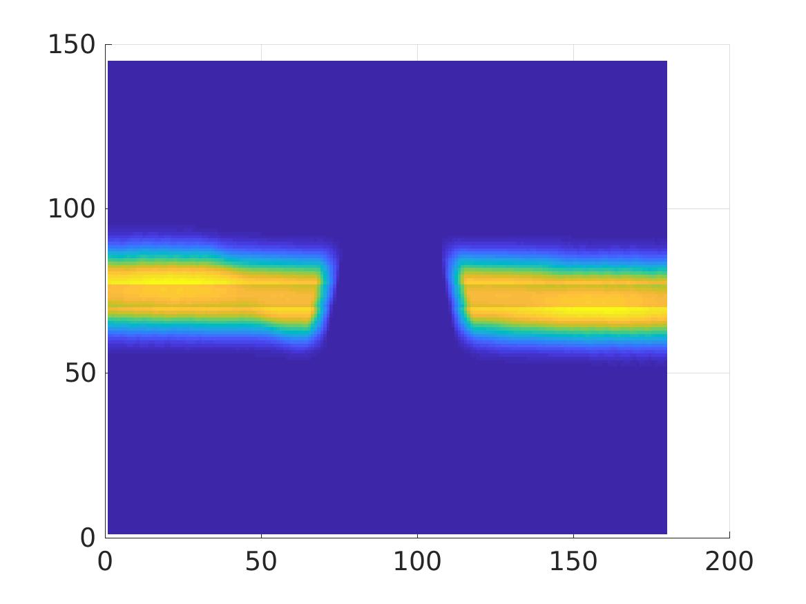
   (d) The incomplete tomographic data, no noise

   

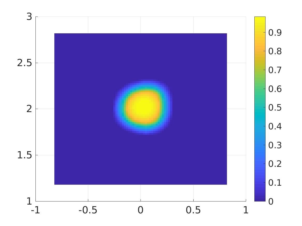
   (e) Post-processed $f^{\mathrm{comp}}$, no noise

   

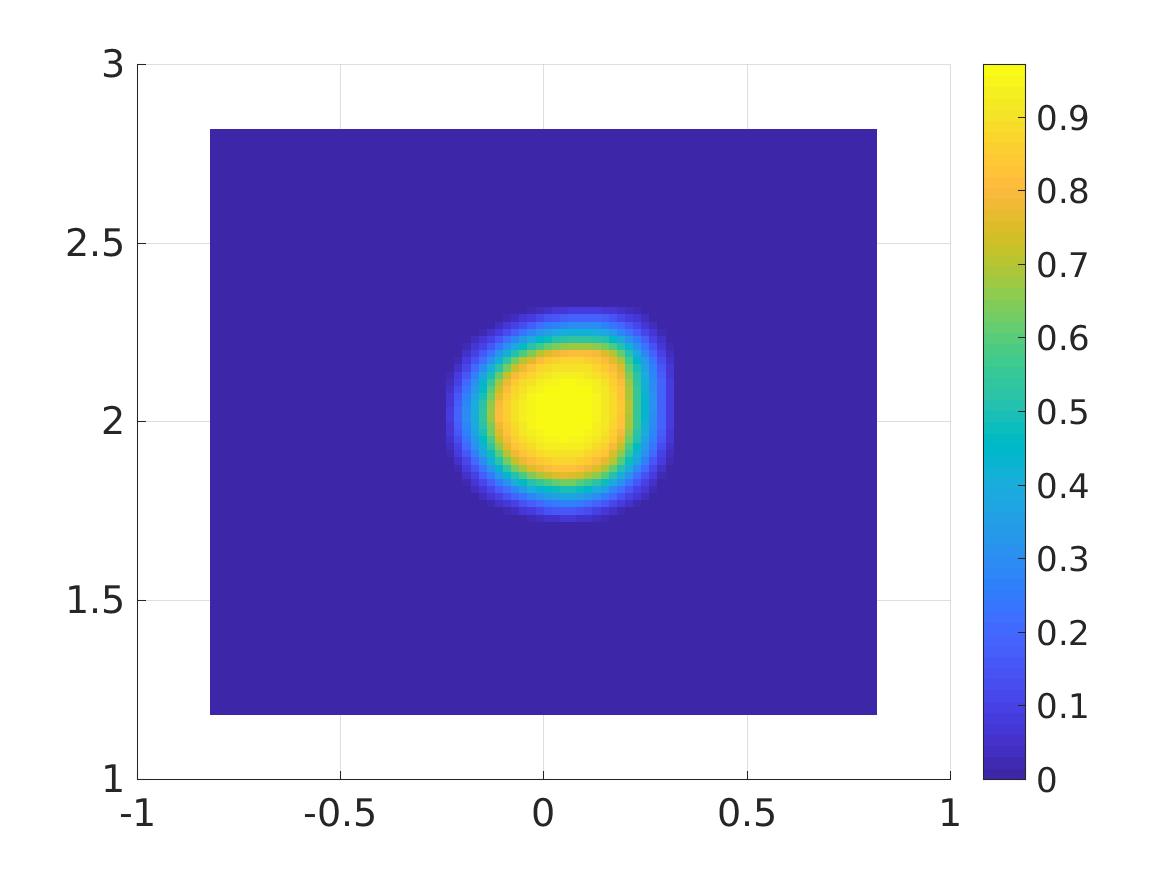
   (f) Post-processed $f^{\mathrm{comp}}_{\delta}$, noise level 90%

   Figure 2: Test 1. The true and reconstructed source functions for circle-shaped smooth inclusion without scattering.

2. Test 2. X-shaped non-smooth inclusion, uniform scattering

   The function $f_{\mathrm{true}}$ is depicted on the Figure 3 (a). We define absorption and scattering coefficients as

   $$\mu_{a}(\mathbf{x})=\left\{\begin{array}[]{rl}0.1&\mbox{if }(x^{2}+y^{2})<0.8,\\ 0&\mbox{otherwise,}\end{array}\right.\mu_{s}(\mathbf{x},\alpha)=\left\{\begin{array}[]{rl}0.01&\mbox{if }(x^{2}+y^{2})<0.8,\\ 0&\mbox{otherwise,}\end{array}\right.$$

   and the constant scattering phase function $K(\mathbf{x},\alpha,\beta)=1/(2d).$ The reconstruction is displayed in Figure 3.

   

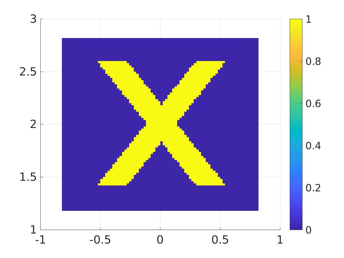
   (a) The function $f_{\rm true}$

   

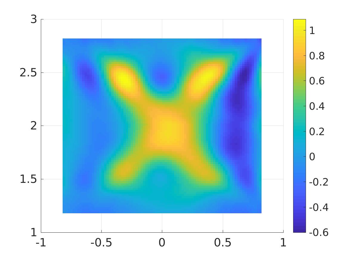
   (b) The reconstructed function $f^{\mathrm{comp}}$, no noise

   

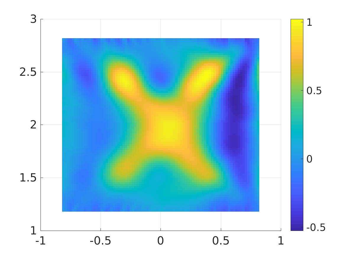
   (c) The reconstructed function $f^{\mathrm{comp}}_{\delta}$, noise 30%

   

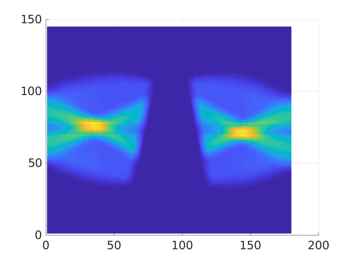
   (d) The incomplete tomographic data, no noise

   

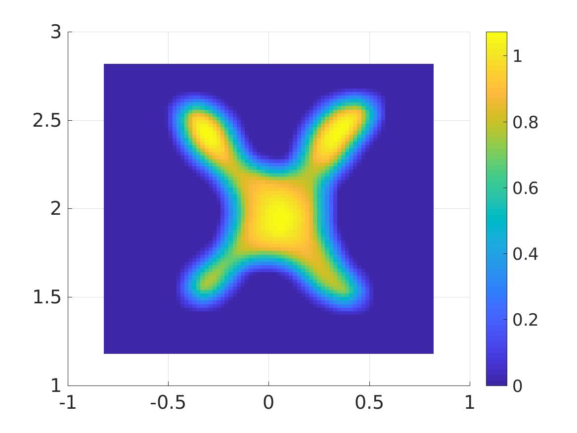
   (e) Post-processed $f^{\mathrm{comp}}$, no noise

   

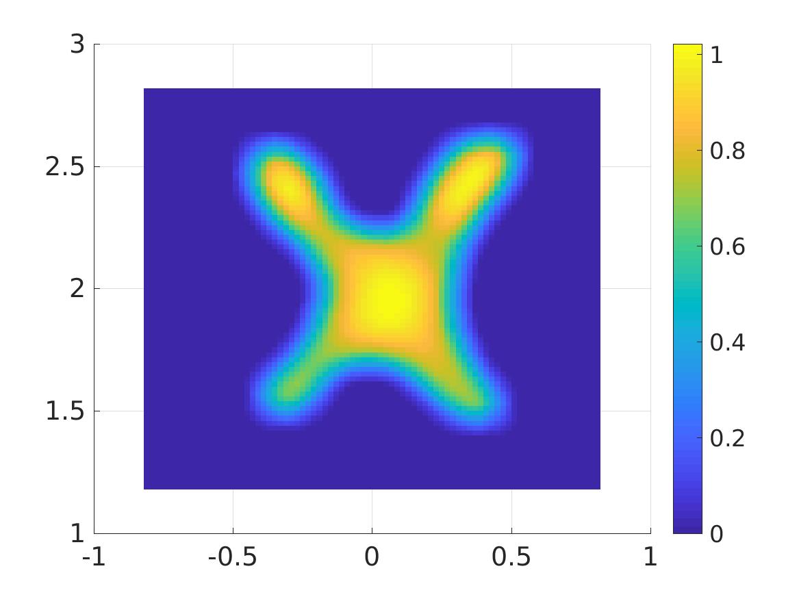
   (f) Post-processed $f^{\mathrm{comp}}_{\delta}$, noise level 30%

   Figure 3: Test 2. The true and reconstructed source functions for for X-shaped non-smooth inclusion, for the case of uniform scattering

3. Test 3. Y-shaped inclusion, strongly forward-peaked scattering

   The function $f_{\mathrm{true}}$ depicted on Figure 4(a) is smooth and compactly supported in the domain. We define absorption and scattering coefficients as

   $$\mu_{a}(\mathbf{x})=\left\{\begin{array}[]{rl}0.15&\mbox{if }(x,y)\in\mathrm{supp}(f_{\mathrm{true}}),\\ 0.1&\mbox{if }(x^{2}+y^{2})<0.8,\\ 0&\mbox{otherwise,}\end{array}\right.$$

   and

   $$\mu_{s}(\mathbf{x})=\left\{\begin{array}[]{rl}0.01&\mbox{if }(x^{2}+y^{2})<0.8,\\ 0&\mbox{otherwise,}\end{array}\right.$$

   and the scattering phase function

   (58) $$K(\mathbf{x},\alpha,\beta)=H(\alpha,\beta)=\frac{1}{2d}\left[\frac{1-g^{2}}{1+g^{2}-2g\cos{(\alpha-\beta})}\right],$$

   where $H(\alpha,\beta)$ is the 2-dimensional Henyey-Greenstein function. In (58), $g=g(x,y)$ is the Henyey-Greenstein factor, it is the smoothed version of the function

   $$\tilde{g}(x,y)=\left\{\begin{array}[]{rl}0.9&\mbox{if }(x^{2}+y^{2})<0.8,\\ 0.5&\mbox{otherwise,}\end{array}\right..$$

   The numerical solution for Test 3 is depicted on Figure 4.

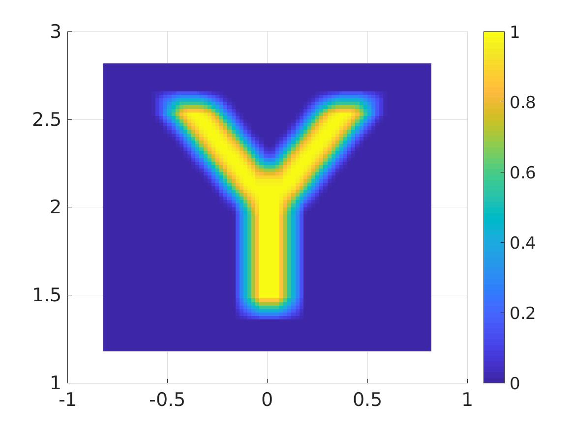
(a) The function $f_{\rm true}$

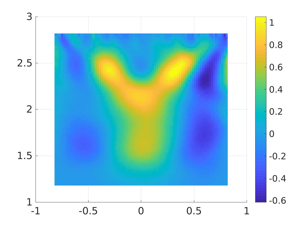
(b) The reconstructed function $f^{\mathrm{comp}}_{\delta}$, noise 60%

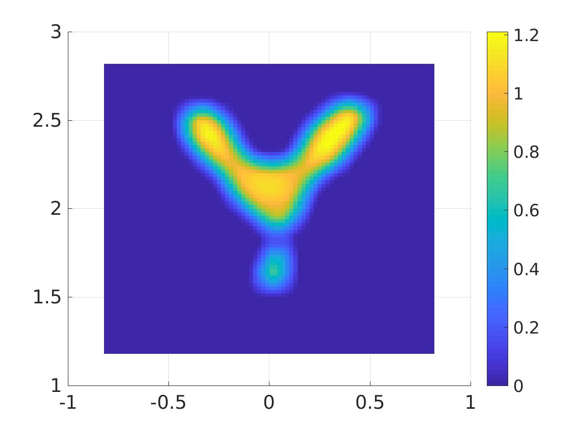
(c) Post-processed $f^{\mathrm{comp}}_{\delta}$, noise level 60%

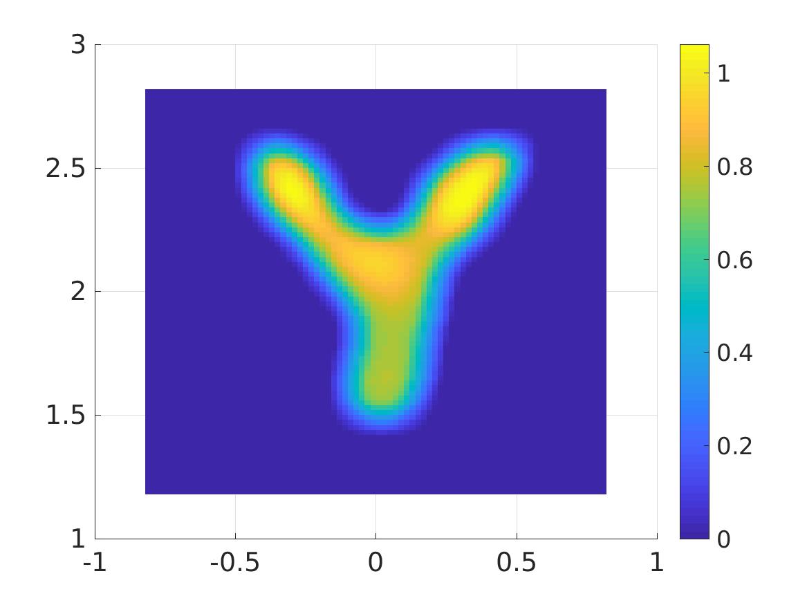
(d) Post-processed $f^{\mathrm{comp}}$, no noise

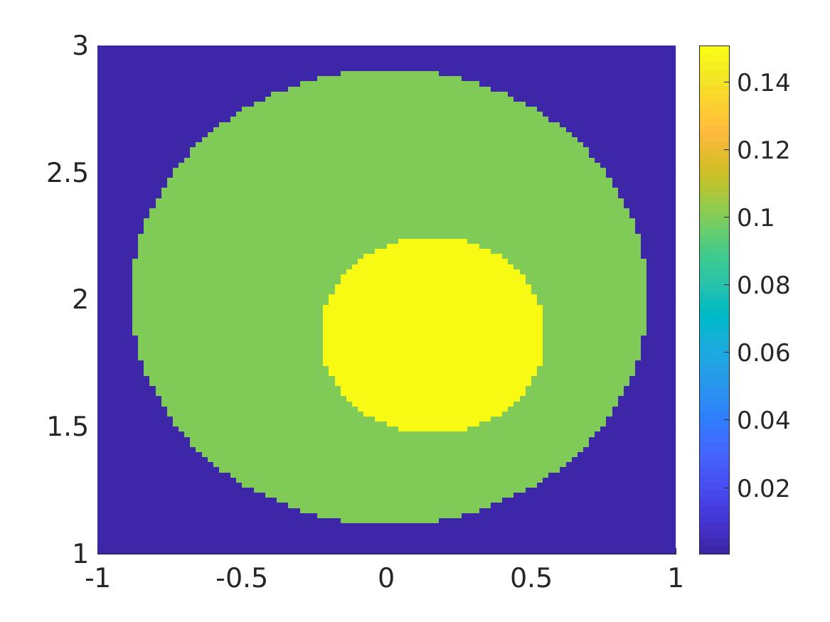
(e) The absorption coefficient

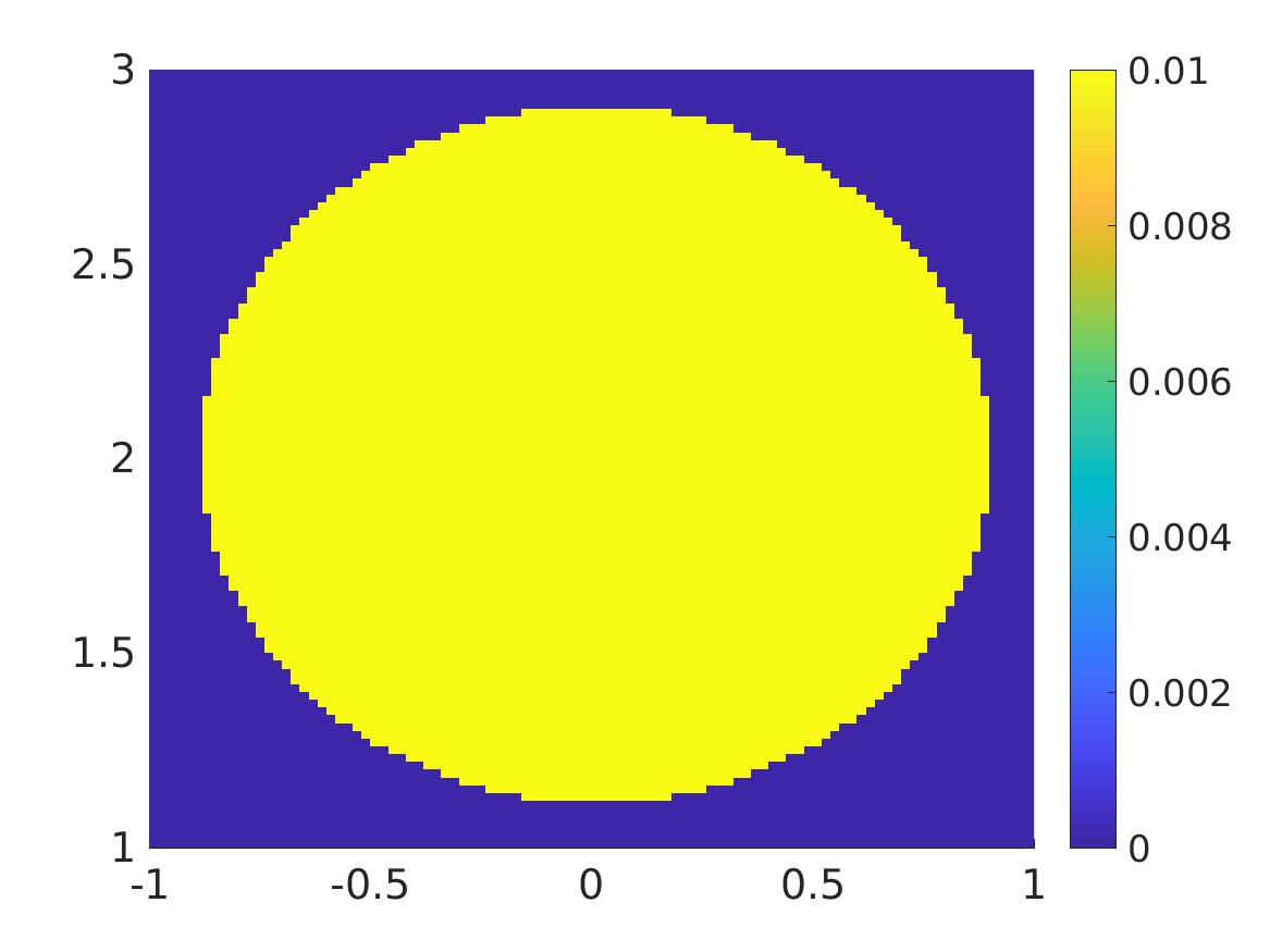
(f) The scattering coefficient

Figure 4: Test 3. The true and reconstructed source functions for Y-shaped inclusion for the case of strongly forward-peaked scattering

Remark 6.1.

In Tests 1 and 2, Figures 2d and 3d are given only for the illustration purpose. They represent the incomplete Radon transform data, obtained by the well-known Radon transform of the function $f^{true}$, in which case $\mu_{a}=\mu_{s}=0.$ The case when the data is available for all $\mathbf{x}$ and $\mathbf{x}_{\alpha}$ such that the set of lines $L(\mathbf{x},\mathbf{x}_{\alpha})$ contains all possible lines intersecting domain $\Omega$ is considered to be the tomographic inverse problem with complete data. In contrast to this, we study the case when, the point source $\mathbf{x}_{\alpha}$ runs along the straight line as shown in Figure 1. In that scenario, the data in our problem is said to be incomplete and Figures 2d and 3d illustrate this. In Test 3 we omit the image representing incomplete Radon data, for the reason that it does not differ qualitatively from Figures 2d and 3d, while the distributions of the absorption and scattering coefficients differ significantly from the previous two tests.

7 Appendix

Theorem 7.1 (Uniqueness and existence of the solution of the Forward Problem).

Consider a rectangular domain $\Omega$, defined in (1). Assume that functions $f,\mu_{a},\mu_{s}\in C^{1}\left(\mathbb{R}^{2}\right),f\in L^{2}\left(\mathbb{R}^{2}\right)$ and the function $K\in C^{1}\left(\mathbb{R}^{2}\times\left[-d,d\right]^{2}\right)$. Also, assume that (4) holds. Then there exists a unique solution $u(\mathbf{x},\alpha)$ of Problem 7 in the domain $\Omega$ such that $u\left(x,y,\alpha\right)\in C^{1}\left(\mathbb{R}\times\left[0,b\right]\times\left[-d,d\right]\right).$ Furthermore, $u(x,y,\alpha)=0$ for $y\in(0,a)$ as well as for sufficiently large $\left|x\right|$.

Proof. Let $L(\mathbf{x},\mathbf{x}_{\alpha})$ be the segment of the straight line connecting points $\mathbf{x}$ and $\mathbf{x}_{\alpha}$. Then for any appropriate function $\phi(\mathbf{x})$

$$\int\displaylimits_{L(\mathbf{x},\mathbf{x}_{\alpha})}\phi(\boldsymbol{\xi})ds_{\boldsymbol{\xi}}=\frac{|\mathbf{x}-\mathbf{x}_{\alpha}|}{y}\int_{0}^{y}\phi\left(\alpha+\frac{w(x-\alpha)}{y},w\right)dw,$$

where $ds_{\boldsymbol{\xi}}$ is the arc length. It follows from (1)-(4) that $u(\mathbf{x},\alpha)=0$ for $y\in(0,a).$ Therefore, the Forward Problem in the domain $\Omega$ is equivalent to

(59) $$u(\mathbf{x},\alpha)=\chi^{-1}(\mathbf{x},\alpha)\frac{|\mathbf{x}-\mathbf{x}_{\alpha}|}{y}\int\displaylimits_{a}^{y}\chi(\mathbf{z})\mu_{s}(\mathbf{z})\int\displaylimits_{-d}^{d}K(\mathbf{z},\alpha,\beta)u(\mathbf{z},\beta)d\beta dw\\ +\chi^{-1}(\mathbf{x},\alpha)\frac{|\mathbf{x}-\mathbf{x}_{\alpha}|}{y}\int\displaylimits_{a}^{y}(f\chi)(\mathbf{z})dw,\hskip 5.0pt$$

and

(60) $$\mathbf{z}(w,x,\alpha)=\left(\alpha+\frac{w(x-\alpha)}{y},w\right),\quad\ln{\chi(\mathbf{x},\alpha)}={\frac{|\mathbf{x}-\mathbf{x}_{\alpha}|}{y}\int_{0}^{y}}(\mu_{a}+\mu_{s})(\mathbf{z})dw.$$

Estimate from the below the absolute value of the first argument in $\mathbf{z}(w,x,\alpha)$ in (60). By (1), (4) and and (60) the left hand side of equation (59) is not zero only if $y\in\left(a,b\right).$ Since in $\mathbf{z}(w,x,\alpha)$ we have $w\in\left(a,y\right),\alpha\in\left(-d,d\right),$ then

(61) $$\left|\alpha+\frac{w(x-\alpha)}{y}\right|\geq\frac{w}{y}\left|x-\alpha\right|-\left|\alpha\right|\geq\frac{a}{b}\left|x\right|-\left(1+\frac{a}{b}\right)\left|\alpha\right|\geq\frac{a}{b}\left|x\right|-\left(1+\frac{a}{b}\right)d.$$

Suppose that $\left|x\right|\geq X$ and $X$ is so large that $1-\frac{1}{X}\left(1+\frac{b}{a}\right)d>\frac{1}{2},\text{ }\frac{a}{2b}X>R.$ Then (61) implies that $\left|\alpha+w(x-\alpha)/y\right|>R.$ Hence, by (1) and (60) the right hand of equation (59) equals zero for $\left|x\right|\geq X.$ Let

$$A\left(u\right):C\left(\mathbb{R}^{2}\times\left[-d,d\right]\right)\rightarrow C\left(\left(\left|x\right|\leq X\right)\times\left[-d,d\right]\times\left[-d,d\right]\right)$$

be the operator in the right hand side of (59). Then (59) can be considered as the equation $u=A\left(u\right)$ with the Volterra-like integral operator, where the “Volterra property” is due to the integration with respect to $y$. Therefore, the latter equation can be solved iteratively, as it is usually done for the Volterra integral equations. It is obvious from the above discussion that all iterates $A\left(u_{n}\right)\left(\mathbf{x},\alpha\right)=0$ for $\left|x\right|\geq X.$ Thus, the solution of equation (59) in the space $C\left(\mathbb{R}^{2}\times\left[-d,d\right]\right)$ exists and is unique. The $C^{1}-$smoothness of this solution with respect to $x,y,\alpha$ obviously follows from the well known convergence estimate for the iterates of a Volterra integral equation. Due to the above mentioned equivalence, this implies uniqueness and existence of the solution of the Forward Problem $\ \square$

The numerical solution of the Forward Problem was performed via the iterative solution of the Volterra-like integral equation (59) for $(\mathbf{x},\alpha)\in\left(\left|x\right|\leq X\right)\times\left[a,b\right]\times\left[-d,d\right]$.

References

- [1] M.A. Anastasio, J. Zhang, D. Modgil and P. J. La Rivière, Application of inverse source concepts to photoacoustic tomography, Inverse Problems, 23 (2007), pp. S21–S35.
- [2] A.B. Bakushinsky, M.Yu. Kokurin and A. Smirnova, Iterative Methods for Ill-Posed Problems: An Introduction, de Gruyter, 2011.
- [3] G. Bal and A. Tamasan, Inverse source problems in transport equations, SIAM J. Math. Anal., 39, 57-76, 2007.
- [4] L. Baudouin, M. de Buhan and S. Ervedoza, Convergent algorithm based on Carleman estimates for the recovery of a potential in the wave equation, SIAM J. Numer. Anal. 55 (2017), pp. 1578–1613.
- [5] L. Beilina and M.V. Klibanov, Approximate Global Convergence and Adaptivity for Coefficient Inverse Problems, Springer, New York, 2012.
- [6] M. Bellassoued and M. Yamamoto, Carleman Estimates and Applications to Inverse Problems for Hyperbolic Systems (Japan: Springer), 2017.
- [7] L. Bourgeois and J. Dardé, A duality-based method of quasi-reversibility to solve the Cauchy problem in the presence of noisy data, Inverse Problems, 26 (2010), 095016.
- [8] L. Bourgeois, D. Ponomarev, and J. Dardé, An inverse obstacle problem for the wave equation in a finite time domain, Inverse Problems and Imaging, 13 (2019) 377-400.
- [9] A. L. Bukhgeim and M. V. Klibanov, Uniqueness in the large of a class of multidimensional inverse problems, Soviet Math. Doklady, 17 (1981), pp. 244–247.
- [10] J.P. Guillement and R.G. Novikov, Inversion of weighted Radon transforms via finite Fourier series weight approximation, Inverse Problems in Science and Engineering, 22, 787-802, 2013.
- [11] J. Heino, S. Arridge, J. Sikora and E. Somersalo, Anisotropic effects in highly scattering media, Physical Review E, 68, 03198, 2003.
- [12] V. Isakov, Inverse Problems for Partial Differential Equations, Third Edition, Springer, New York, 2017.
- [13] M. Jiang, T. Zhou, J. Cheng, W. Cong and G. Wang, Image reconstruction for bioluminescence tomography from partial measurement, Opt. Express, 15 (2007), pp. 11095–11116.
- [14] S. I. Kabanikhin, A. D. Satybaev, and M. A. Shishlenin, Direct Methods of Solving Inverse Hyperbolic Problems, VSP, Utrecht, 2005.
- [15] M. V. Klibanov, Inverse problems and Carleman estimates, Inverse Problems, 8 (1992), pp. 575–596.
- [16] M. V. Klibanov and A. Timonov, Carleman Estimates for Coefficient Inverse Problems and Numerical Applications, Inverse and Ill-Posed Problems Series, VSP, Utrecht, 2004.
- [17] M. V. Klibanov, Carleman estimates for global uniqueness, stability and numerical methods for coefficient inverse problems, J. Inverse and Ill-Posed Problems, 21 (2013), pp. 477–560.
- [18] M. V. Klibanov and N. T. Thành, Recovering of dielectric constants of explosives via a globally strictly convex cost functional, SIAM J. Appl. Math., 75 (2015), pp. 518–537.
- [19] M. V. Klibanov, Carleman estimates for the regularization of ill-posed Cauchy problems, Applied Numerical Mathematics, 94 (2015), pp. 46–74.
- [20] M. V. Klibanov, Convexification of restricted Dirichlet to Neumann map, J. Inverse and Ill-Posed Problems, 25 (2017), pp. 669–685.
- [21] M. V. Klibanov, A. E. Kolesov, A. Sullivan, and L. Nguyen, A new version of the convexification method for a 1-D coefficient inverse problem with experimental data, Inverse Problems, 34 (2018), 115014.
- [22] M. V. Klibanov, J. Li, and W. Zhang, Electrical impedance tomography with restricted dirichlet-to-neumann map data, Inverse Problems, 35 (2019), 35005.
- [23] M. V. Klibanov and L. H. Nguyen, PDE-based numerical method for a limited angle X-ray tomography, Inverse Problems, 35 (2019), 045009.
- [24] A. D. Klose, V. Ntziachristos, and A. H. Hielscher, The inverse source problem based on the radiative transfer equation in optical molecular imaging, Journal of Computational Physics, 202 (2005), pp. 323 – 345.
- [25] R. Lattes and J. L. Lions, The Method of Quasireversibility: Applications to Partial Differential Equations, Elsevier, New York, 1969.
- [26] Q. Li and L. H. Nguyen, Recovering the initial condition of parabolic equations from lateral Cauchy data via the quasi-reversibility method,, preprint, arXiv:1902.07637, (2019).
- [27] A. K. Louis, Incomplete data problems in x-ray computerized tomography, Numerische Mathematik, 48 (1986), pp. 251–262.
- [28] F. Natterer, The Mathematics of Computerized Tomography, SIAM, Philadelphia, 2001.
- [29] F. Natterer, Inversion of the Attenuated Radon Transform,Inverse Problems, 17, 113-119, 2001.
- [30] L. H. Nguyen, Q. Li, and M. V. Klibanov, A convergent numerical method for a multi-frequency inverse source problem in inhomogenous media, preprint, arXiv:1901.10047, (2019).
- [31] R.G. Novikov, An inversion formula for the attenuated X-ray transformation, Ark. Mat., 40, 145-167, 2002.
- [32] A.A. Samarskii, The Theory of Difference Schemes, Marcel Dekker, Inc., New York.
- [33] A.J. Silva Neto and M.N. Özişik, An inverse problem of simultaneous estimation of radiation phase function, albedo and optical thickness, Journal of Quantitative Spectroscopy and Radiative Transfer, 53 (1995), pp. 397 – 409.
- [34] P. Stefanov and G. Uhlmann, An inverse source problem in optical molecular imaging, Analysis and PDE, 1, 115-126, 2008.