Multi-outcome homodyne detection in a coherent-state light interferometer

Abstract

The Cramér-Rao bound plays a central role in both classical and quantum parameter estimation, but finding the observable and the resulting inversion estimator that saturates this bound remains an open issue for general multi-outcome measurements. Here we consider multi-outcome homodyne detection in coherent-light Mach-Zehnder interferometer and construct a family of inversion estimators that almost saturate the Cramér-Rao bound over the whole range of phase interval. This provides a clue on constructing optimal inversion estimators for phase estimation and other parameter estimation in any multi-outcome measurement.

I Introduction

Interference of light fields is important in astronomy Born ; Caves , spectroscopy Wineland ; Leibfried , and various fields of quantum technology Dowling . For instance, in optical lithography Boto , the light-intensity measurement gives rise to an oscillatory interferometric signal $\propto\sin^{2}(\phi/2)$ or $\cos^{2}(\phi/2)$, which exhibits the fringe resolution $\lambda/2$, determined by the wavelength $\lambda$. This is often referred to the classical resolution limit of interferometer, or the Rayleigh resolution criterion in optical imaging Boto . To beat this classical limit, it has been proposed to use $N$-photon entangled states $(|N,0\rangle+|0,N\rangle)/\sqrt{2}$ Boto ; Mitchell ; Walther ; Chen ; Afek , which results in the resolution $\lambda/(2N)$, i.e., $N$-times improvement beyond the classical resolution limit. However, the $N$-photon entangled states are difficult to prepare and are subject to photon losses Braun ; Dorner ; Zhang . In the absence of quantum entanglement, the super-resolution can be also attainable from different types of measurement schemes, such as coincidence photon counting Resch , parity detection Gao ; Cohen , and homodyne detection with post-processing Andersen .

To realize a high-precision measurement of an unknown phase $\phi$, an optimal measurement scheme with a proper choice of data processing is important to improve both the resolution and the phase sensitivity Bevington ; Dowling . Given a phase-encoded state and a properly chosen observable $\hat{\Pi}$, the ultimate phase estimation precision is determined by the Cramér-Rao lower bound (CRB) Helstrom ; Braunstein ; Braunstein2 ; Paris1 , i.e., $\delta\phi\geq\delta\phi_{\mathrm{CRB}}=1/\sqrt{F(\phi)}$, where $F(\phi)$ is the classical Fisher information (CFI), dependent on the measurement probabilities. To saturate the CRB, it requires complicated data-processing techniques such as maximal likelihood estimation or Bayesian estimation YMK ; Pezze . However, they lack physical transparency and require a lot of computational resources. By contrast, the simplest data processing is to equate the theoretical expectation value $\langle\hat{\Pi}\rangle_{\phi}=f(\phi)$ with the experimentally measured value $\Pi_{\exp}$, which gives a simple inversion estimator $\phi_{\mathrm{inv}}\equiv f^{-1}(\Pi_{\exp})$ to the unknown phase $\phi$, with a precision determined by the error-propagation formula:

$$\delta\phi=\frac{\Delta\hat{\Pi}}{\left|\partial\langle\hat{\Pi}\rangle_{\phi}/\partial\phi\right|}.$$ (1)

Here $\Delta\hat{\Pi}\equiv(\langle\hat{\Pi}^{2}\rangle_{\phi}-\langle\hat{\Pi}\rangle_{\phi}^{2})^{1/2}$ is the root-mean-square fluctuation of the observable $\hat{\Pi}$. Due to its physical transparency and computational simplicity, the inversion estimator has been widely used in various phase estimation schemes. Moreover, for binary-outcome measurements (such as parity detection Bollinger ; Gerry2 ; Gerry2a ; Gerry2b ; Anisimov ; Chiruvelli ; Seshadreesan , single-photon detection Cohen , and on-off measurement), the inversion estimator asymptotically approaches the maximum likelihood estimator Feng ; Paris ; Jin and hence saturates the CRB within the whole phase interval, e.g., $\phi\in[-\pi,\pi]$. However, for general multi-outcome measurements, the performance of the inversion estimator depends strongly on the chosen observable $\hat{\Pi}$ and usually cannot saturate the CRB Andersen . Therefore, an important problem in high-precision phase estimation is to find an optimal inversion estimator that saturates the CRB. At present, this problem remains open.

In this paper, we investigate the performance of the inversion estimator in multi-outcome measurements and report some interesting findings. We begin with a binary observable, i.e., a multi-outcome measurement with only two different eigenvalues. Such a binary observable plays a key role in achieving deterministic super-resolution in a Mach-Zehnder interferometer fed by a coherent-state light in a recent experiment Andersen . We find that using a binary observable to construct the inversion estimator is equivalent to binarizing the original multi-outcome measurement into an effective binary-outcome one. As a result, the precision of the inversion estimator saturates the CRB determined by the CFI of this binary-outcome measurement and is independent of the choices of the eigenvalues. We show that the observable adopted in Ref. Andersen belongs to this class. Next, we consider the homodyne detection of Ref. Andersen as a paradigmatic example to study the dependence of the precision of the inversion estimator on the observable. Surprisingly, we find that when the neighboring eigenvalues of the observable have alternating signs, the resulting inversion estimator is nearly optimal, i.e., its precision almost saturates the CRB. This may provide a clue on constructing optimal inversion estimators for phase estimation and other parameter estimation (e.g., optical angular displacements Zhao ; Cen ; Wang ; Xu ; Qiang ).

II Quantum phase estimation with a multi-outcome measurement

For a $(N+1)$-outcome measurement, the most general observable is

$$\hat{\Pi}=\sum_{k=0}^{N}\mu_{k}\hat{\Pi}_{k},$$ (2)

where $\mu_{k}$ ($\hat{\Pi}_{k}$) is the eigenvalue (projector) associated with the $k$th outcome. The output signal is the average of the observable $\hat{\Pi}$ with respect to the phase-encoded state $\hat{\rho}(\phi)$:

$$\langle\hat{\Pi}\rangle_{\phi}=\sum_{k=0}^{N}\mu_{k}P(k|\phi)\approx\sum_{k=0}^{N}\mu_{k}\frac{{\mathcal{N}}_{k}}{{\mathcal{N}}},$$ (3)

where $P(k|\phi)=\mathrm{Tr}[\hat{\rho}(\phi)\hat{\Pi}_{k}]$ is the conditional probability of the $k$th outcome, which can be measured by the occurrence frequency ${\mathcal{N}}_{k}/{\mathcal{N}}$. Specially, one can perform ${\mathcal{N}}$ independent measurements at each phase shift $\phi\in[-\pi,\pi]$ and record the occurrence numbers $\{{\mathcal{N}}_{k}\}$. For large enough ${\mathcal{N}}$, $P(k|\phi)\approx{\mathcal{N}}_{k}/{\mathcal{N}}$. Numerical simulation of a special kind of multi-outcome measurement will be shown at the end of this work.

We begin with a binary observable – the multi-outcome measurement with only two different eigenvalues. Without losing generality, we take $\mu_{N}=\mu_{N-1}=\cdots=\mu_{1}$, then we can use $\hat{\Pi}_{k}\hat{\Pi}_{k^{\prime}}=\delta_{kk^{\prime}}\hat{\Pi}_{k}$ to obtain

$$\langle\hat{\Pi}\rangle_{\phi} = \mu_{0}P(0|\phi)+\mu_{1}P(\emptyset|\phi),$$

$$\langle\hat{\Pi}^{2}\rangle_{\phi} = \mu_{0}^{2}P(0|\phi)+\mu_{1}^{2}P(\emptyset|\phi),$$

where $P(\emptyset|\phi)\equiv\sum_{k=1}^{N}P(k|\phi)$ and $P(0|\phi)=1-P(\emptyset|\phi)$. Therefore, the phase sensitivity of the inversion estimator based on the binary observable $\hat{\Pi}$ is independent of the eigenvalues $\mu_{0}$ and $\mu_{1}$:

$$(\delta\phi)^{2}=\frac{P(\emptyset|\phi)P(0|\phi)}{\left[P^{\prime}(\emptyset|\phi)\right]^{2}},$$ (4)

where $P^{\prime}\equiv\partial P/\partial\phi$. Interestingly, if we binarize the $N+1$ outcomes into two outcomes $0$ and “$\emptyset$”, i.e., we regard the outcomes $1,2,\cdots,N$ as a single outcome “$\emptyset$”, then $P(\emptyset|\phi)$ is just the conditional probability for “$\emptyset$” and the CFI of this effective binary measurement coincides with $1/(\delta\phi)^{2}$. In other words, the phase sensitivity $\delta\phi$ of the inversion estimator based on the binary observable $\hat{\Pi}$ always saturates the CRB of the effective binary-outcome measurement Feng . Since this effective binary-outcome measurement is obtained from the original multi-outcome measurement by coarse-graining, its CFI is smaller than the CFI of the original one:

$$F(\phi)\equiv\sum_{k=0}^{N}\frac{\left[P^{\prime}(k|\phi)\right]^{2}}{P(k|\phi)}.$$ (5)

As a result, $\delta\phi$ cannot saturate the CRB of the original multi-outcome measurement $\delta\phi_{\mathrm{CRB}}\equiv 1/\sqrt{F(\phi)}$ Helstrom ; Braunstein ; Braunstein2 ; Paris1 . Therefore, it is important to find an optimal choice of eigenvalues $\{\mu_{k}\}$ such that $\delta\phi=\delta\phi_{\mathrm{CRB}}$.

The above results are applicable to an arbitrary measurement scheme and arbitrary input state. In the following, we consider the homodyne detection at one port of Mach-Zehnder interferometer with a coherent-state input Andersen as a paradigmatic example to illustrate these results. Interestingly, we find a nearly optimal observable that almost saturates the CRB for all $\phi\in[-\pi,\pi]$.

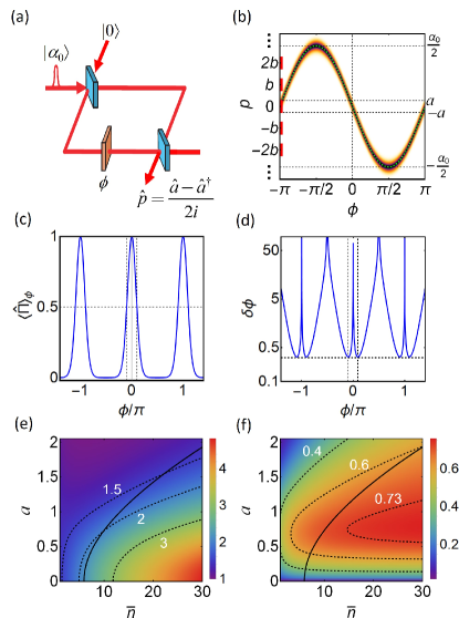
Figure 1: (a) Homodyne detection at one port of the coherent-state interferometer, equivalent to measuring quadrature operator $\hat{p}$ with respect to the output state. (b) Conditional probability $P(p|\phi)$ against the phase shift $\phi$ and the measured quadrature $p$, given by Eq. (11), and the post-processing method by separating the measured data into several bins Andersen , where the bin’s center is $kb$ (for $k=0$, $\pm 1$, …$\pm k_{f}$) and the width is $2a$, equivalent to a multi-outcome measurement. (c) and (d): Output signal $\langle\hat{\Pi}\rangle_{\phi}$ and phase sensitivity $\delta\phi$ for $k_{f}=0$, equivalent to a binary-outcome measurement. The vertical lines determine the resolution and the best sensitivity, measured respectively by the full width at half maximum ($\mathrm{FWHM}$) and the best sensitivity $\delta\phi_{\min}$. (e) and (f): Density plots of the ratios $\frac{2\pi/3}{\mathrm{FWHM}}$ and $\frac{1/\sqrt{\bar{n}}}{\delta\phi_{\min}}$ as functions of the average photon number $\bar{n}$ $(=\alpha_{0}^{2})$ and the bin size $a$. Dashed lines: contours of the two ratios. Solid lines and below: a region that the visibility of the signal $\geq 90\%$.

As depicted by Fig. 1(a), a coherent state $|\alpha_{0}\rangle$ and a vacuum state $|0\rangle$ are injected from the input ports. The output state is given by $|\psi_{\mathrm{out}}(\phi)\rangle=\hat{U}(\phi)|\psi_{\mathrm{in}}\rangle$, where $\hat{U}(\phi)$ is an unitary operator

$$\hat{U}(\phi)=\exp\left(-i\frac{\pi}{2}\hat{J}_{y}\right)\exp\left(-i\phi\hat{a}^{{\dagger}}\hat{a}\right)\exp\left(-i\frac{\pi}{2}\hat{J}_{y}\right),$$ (6)

which represents a sequence actions of the 50:50 beamsplitter at the output port Gerrybook , the phase accumulation at one of the two paths, and the 50:50 beamsplitter at the input port. For brevity, we have introduced Schwinger’s representation of the angular momentum $\hat{J}=\frac{1}{2}(\hat{a}^{{\dagger}},\hat{b}^{{\dagger}})\hat{\sigma}\binom{\hat{a}}{\hat{b}}$, where $\hat{a}^{{\dagger}}$ ($\hat{a}$) and $\hat{b}^{{\dagger}}$ ($\hat{b}$) denote the creation (annihilation) operators of the two field modes and $\hat{\sigma}=(\hat{\sigma}_{x},\hat{\sigma}_{y},\hat{\sigma}_{z})$ the Pauli matrix.

In general, a homodyne detection at one of two output ports gives the measured quadrature $p\in(-\infty,\infty)$, with the conditional probability

$$P(p|\phi)=\int_{-\infty}^{\infty}dx\int_{-\infty}^{\infty}dX\int_{-\infty}^{\infty}dPW_{\mathrm{out}}(\alpha,\beta;\phi),$$ (7)

where $\alpha=x+ip$ ($x$, $y\in\mathbb{R}$) and $\beta=X+iP$ ($X$, $P\in\mathbb{R}$), and $W_{\mathrm{out}}$ is the Wigner function of the output state Seshadreesan2 ; Tan ,

$$W_{\mathrm{out}}(\alpha,\beta;\phi)=W_{\mathrm{in}}(\tilde{\alpha}_{\phi},\tilde{\beta}_{\phi}),$$ (8)

with

$$\left\{\begin{array}[]{l}\tilde{\alpha}_{\phi}=\alpha\frac{e^{i\phi}-1}{2}+\beta\frac{e^{i\phi}+1}{2},\\ \tilde{\beta}_{\phi}=-\alpha\frac{e^{i\phi}+1}{2}-\beta\frac{e^{i\phi}-1}{2}.\end{array}\right.$$ (9)

Note that Eqs. (8) and (9) are valid for the two-path interferometer described by $\hat{U}(\phi)$, independent from the input state and the measurement scheme.

For the coherent-state input $|\psi_{\mathrm{in}}\rangle=|\alpha_{0}\rangle\otimes|0\rangle$, the Wigner function is given by Gerrybook

$$W_{\mathrm{in}}(\alpha,\beta)=\left(\frac{2}{\pi}\right)^{2}e^{-2|\alpha-\alpha_{0}|^{2}}e^{-2|\beta|^{2}}.$$ (10)

Replacing $(\alpha,\beta)$ by $(\tilde{\alpha}_{\phi},\tilde{\beta}_{\phi})$, one can obtain the Wigner function of the output state, as shown by Eq. (8). For $\alpha_{0}=\sqrt{\bar{n}}\in\mathbb{R}$, we obtain the probability to detecting an outcome $p$,

$$P(p|\phi)=\sqrt{\frac{2}{\pi}}\exp\left[-2\left(p+\frac{\alpha_{0}}{2}\sin\phi\right)^{2}\right],$$ (11)

in agreement with our previous result Feng . In Fig. 1(b), we show density plot of $P(p|\phi)$ against the phase shift $\phi$ and the measured quadrature $p$. The green dashed line is given by the equation $p=-\alpha_{0}\sin(\phi)/2$, indicating the peak of $P(p|\phi)$. The commonly used observable in a traditional homodyne measurement is given by $\hat{\Pi}=\int_{-\infty}^{\infty}\!p|p\rangle\langle p|dp$, where $\hat{p}|p\rangle=p|p\rangle$ and $\hat{p}\equiv(\hat{a}-\hat{a}^{\dagger})/(2i)$. The output signal is the average of this observable $\langle\hat{\Pi}\rangle_{\phi}=\int_{-\infty}^{\infty}\!dppP(p|\phi)\propto\sqrt{\bar{n}}\sin\phi$, which exhibits the full width at half maximum ($\mathrm{FWHM}$)$\ 2\pi/3$, and hence the Rayleigh limit in fringe resolution. The resolution can be improved by choosing a suitable observable Andersen .

III Binary-outcome homodyne detection

We first consider the binary-outcome homodyne detection, where the measured data has been divided into two bins Andersen : $p\in[-a,a]$ as an outcome, denoted by “$+$”, and $p\notin[-a,a]$ as an another outcome “$-$”, with the bin size $2a$. Using Eq. (11), it is easy to obtain the conditional probabilities of the outcomes “$\pm$”, namely

$$P(+|\phi)=\int_{-a}^{+a}dpP(p|\phi)=\frac{1}{2}\mathrm{Erf}\left[g_{-}(\phi),g_{+}(\phi)\right],$$ (12)

and hence $P(-|\phi)=1-P(+|\phi)$. Here, $\mathrm{Erf}\left[x,y\right]=\mathrm{erf}(y)-\mathrm{erf}(x)$ denotes a generalized error function, and

$$g_{\pm}(\phi)=\sqrt{2}\left(\frac{\alpha_{0}}{2}\sin\phi\pm a\right).$$ (13)

Obviously, this is a binary-outcome measurement with the observable $\hat{\Pi}=\mu_{+}\hat{\Pi}_{+}+\mu_{-}\hat{\Pi}_{-}$, where $\hat{\Pi}_{+}=\int_{-a}^{+a}|p\rangle\langle p|dp$ and $\hat{\Pi}_{-}=\hat{1}-\hat{\Pi}_{+}$. The signal is the average of $\hat{\Pi}$

$$\left\langle\hat{\Pi}\right\rangle_{\phi}=\mu_{+}P(+|\phi)+\mu_{-}P(-|\phi),$$ (14)

where $\langle\hat{\Pi}_{\pm}\rangle_{\phi}=P(\pm|\phi)$. According to Eq. (4), we obtain the phase sensitivity of the inversion estimator:

$$\delta\phi=\frac{\sqrt{P(+|\phi)P(-|\phi)}}{\left|P^{\prime}(+|\phi)\right|},$$ (15)

which is independent of the eigenvalues $\mu_{\pm}$ of the binary observable $\hat{\Pi}$. The CFI of this binary-outcome measurement is given by Feng ; Paris ; Jin

$$F(\phi)=\sum_{k=\pm}\frac{\left[P^{\prime}(k|\phi)\right]^{2}}{P(k|\phi)}=(\delta\phi)^{-2},$$ (16)

where, in the last step, we have used the relation $P(+|\phi)+P(-|\phi)=1$. Therefore, the sensitivity $\delta\phi$ of the inversion estimator based on the binary observable $\hat{\Pi}$ always saturates the CRB of the binary-outcome measurement Feng ; Paris ; Jin .

In Figs. 1(c) and 1(d), we take $\mu_{+}=1/\mathrm{erf}(\sqrt{2}a)$ and $\mu_{-}=0$ to show the signal and the sensitivity as functions of $\phi$, where $\mathrm{erf}(\sqrt{2}a)$ is a normalization factor Andersen . The vertical lines determine the resolution and the best sensitivity $\delta\phi_{\min}=1/\sqrt{F(\phi_{\min})}$. From Figs. 1(e) and 1(f), one can find that a higher resolution with the $\mathrm{FWHM}\sim\pi/\sqrt{\bar{n}}$, can be obtained as the bin size $a\rightarrow 0$. However, the best sensitivity occurs as $a\geq 1/2$. Therefore, as a trade-off, one can simply take $a=(\Delta\hat{p})_{|\alpha\rangle}=1/2$ Andersen , for which both the resolution and the sensitivity scale inversely with $\sqrt{\bar{n}}$. Numerically, it has been shown that the best sensitivity can reach $\delta\phi_{\min}\sim 1.37/\sqrt{\bar{n}}$ Andersen .

We now investigate the visibility of the interferometric signal and its relationship with $a$ and $\bar{n}$ that have not been addressed by Ref. Andersen . From Fig.1(c), one can note that the visibility can be determined by

$$V=\frac{\left\langle\hat{\Pi}\right\rangle_{\phi=0}-\left\langle\hat{\Pi}\right\rangle_{\phi=\pi/2}}{\left\langle\hat{\Pi}\right\rangle_{\phi=0}+\left\langle\hat{\Pi}\right\rangle_{\phi=\pi/2}},$$ (17)

where $\phi=\pm\pi/2$ denote the dark points of the signal. Using Eqs. (12) and (14), we can easily obtain an analytical result of the visibility, which gives a relation between $a$ and $\bar{n}$ for a given $V$. The solid line of Fig. 1(e) corresponds to $V=0.9$ and a region below it indicates $V>0.9$. Our numerical results show that the visibility is larger than $90\%$ only when the average number of photons is not too small (at least $\bar{n}>5.8$).

IV Multi-outcome homodyne detection

To proceed, let us consider the multi-outcome case by separating the measured quadrature into several bins Andersen , i.e., treating $p\in[b_{k}-a,b_{k}+a]$ as an outcome $k$, where $b_{k}$ is center of each bin. When $p$ does not lie within any bin, then we identify $p$ as outcome “$-$”. The occurrence probability of the $k$-th outcome is

$$P(k|\phi) =\int_{b_{k}-a}^{b_{k}+a}dpP(p|\phi)$$

$$=\frac{1}{2}\mathrm{Erf}\left[g_{-}(\phi)+\sqrt{2}b_{k},g_{+}(\phi)+\sqrt{2}b_{k}\right],$$ (18)

where $g_{\pm}(\phi)$ is defined in Eq. (13). The occurrence probability for the outcome “$-$” is simply given by $P(-|\phi)=1-\sum_{k}P(k|\phi)$. According to Distante et al. Andersen , one can take $b_{k}=kb$ with the integers $k=0$, $\pm 1$, $\cdots$, $\pm k_{f}$ and a factor $b$ to be determined, so the total number of the outcomes is $2(k_{f}+1)$. For a given $b>2a$, the overlap of the conditional probabilities between neighbour outcomes is vanishing, and $k_{f}b\sim\alpha_{0}/2$ [see Fig. 1(b)]. For large enough $\bar{n}=\alpha_{0}^{2}$ and $b$ ($>2a$), we take $k_{f}=[\alpha_{0}/(2b)]$ such that the outcomes for $|k|>k_{f}$ give almost vanishing contribution, where $[x]$ is the integer closest to $x$.

In Fig. 2, we take $\alpha_{0}=\sqrt{200}$, $a=1/2$, and $b=3.8$ to show the occurrence probabilities as function of $\phi$. Here, the total number of the outcomes $2(k_{f}+1)=6$, since $k_{f}=2$. The visibility of $P(0|\phi)$ is similar to the binary-outcome problem and is larger than $90\%$ as long as $\bar{n}=\alpha_{0}^{2}>5.8$. Numerical simulations of the occurrence probabilities are shown using random numbers ranged from $0$ to $1$ (see below).

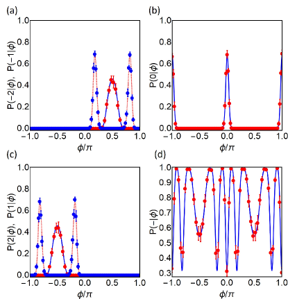
Figure 2: Conditional probabilities $P(k|\phi)$ for $k=0$, $\pm 1$, …, $\pm k_{f}$, and $P(-|\phi)=1-\sum_{k}P(k|\phi)$. The parameters: $\bar{n}=200$, $a=1/2$, $b=3.8$, and hence the total number of the outcomes $2(k_{f}+1)=6$, since $k_{f}=2$ (see text). Left panel: $P(\pm 2|\phi)$ for the blue solid lines, and $P(\pm 1|\phi)$ for the red dashed lines. Numerical simulations: averaged occurrence frequency ${\mathcal{N}}_{k}/{\mathcal{N}}$ (the solid circles) and its standard derivation (the bars) of each outcome after $M=10$ replicas of ${\mathcal{N}}=200$ independent measurements.

The observable corresponding to this multi-outcome homodyne detection can be written as $\hat{\Pi}=\mu_{-}\hat{\Pi}_{-}+\sum_{k}\mu_{k}\hat{\Pi}_{k}$, where $\hat{\Pi}_{k}\equiv\int_{b_{k}-a}^{b_{k}+a}|p\rangle\langle p|dp$ and $\hat{\Pi}_{-}\equiv\hat{1}-\sum_{k}\hat{\Pi}_{k}$, with the eigenvalues $\{\mu_{k}\}$ and $\mu_{-}$. The signal is the average of $\hat{\Pi}$:

$$\left\langle\hat{\Pi}\right\rangle_{\phi}=\sum_{k=-k_{f}}^{k_{f}}\mu_{k}P(k|\phi)+\mu_{-}P(-|\phi),$$ (19)

Previously, Distante et al. Andersen have derived the signal and the sensitivity by taking $\mu_{k}=1/\mathrm{erf}(\sqrt{2}a)$ and $\mu_{-}=0$. For arbitrary $\mu_{k}=\mu_{+}$ and $\mu_{-}=0$, it is easy to reduce the signal as $\langle\hat{\Pi}\rangle_{\phi}=\mu_{+}-(\mu_{+}-\mu_{-})P(-|\phi)$. Furthermore, the sensitivity is found independent on the values of $\mu_{\pm}$; see Eq. (4). In Figs. 3(a) and 3(b), we simply take $\mu_{k}=\mu_{+}=1$ and $\mu_{-}=0$ to show the signal $\langle\hat{\Pi}\rangle_{\phi}=1-P(-|\phi)$ and the sensitivity against $\phi$. Similar to Ref. Andersen , the signal exhibits a multi-fold oscillatory pattern, with the peaks located at

$$\phi_{k}=\arcsin\left(\frac{2b_{k}}{\alpha_{0}}\right),$$ (20)

and also $\pi-\phi_{k}$. If the bin’s center $b_{k}=kb$ and $|k|<k_{f}$, it is easy to obtain $\phi_{k}\approx 2kb/\alpha_{0}$ and hence the first dark point of the signal $\phi_{\mathrm{dark}}\approx\phi_{\pm 1}/2\approx\pm b/\alpha_{0}$; see the vertical lines of Fig. 3(a).

When all $\{\mu_{k}\}$ are the same, we obtain a binary observable $\hat{\Pi}$ and the sensitivity is similar to Eq. (4),

$$\delta\phi=\frac{\sqrt{P(+|\phi)P(-|\phi)}}{|P^{\prime}(-|\phi)|}\geq\frac{1}{\sqrt{F(\phi)}},$$ (21)

where $P(+|\phi)\equiv\sum_{k}P(k|\phi)=1-P(-|\phi)$, and $F(\phi)$ is the CFI of the multi-outcome homodyne measurement,

$$F(\phi)=\sum_{k=-k_{f}}^{k_{f}}\frac{\left[P^{\prime}(k|\phi)\right]^{2}}{P(k|\phi)}+\frac{\left[P^{\prime}(-|\phi)\right]^{2}}{P(-|\phi)}.$$ (22)

In Fig. 3(b), we show the sensitivity $\delta\phi$ and its ultimate lower bound $\delta\phi_{\mathrm{CRB}}=1/\sqrt{F(\phi)}$ against $\phi$. One can see that the sensitivity $\delta\phi$ diverges at certain values of $\phi$ (e.g., $\phi_{\mathrm{dark}}\approx\pm b/\alpha_{0}$), but $\delta\phi_{\mathrm{CRB}}$ does not (see the red dashed line). The singularity of $\delta\phi$ means that complete no phase information can be inferred. Usually, it takes place when the slope of signal is vanishing, i.e., $P^{\prime}(-|\phi)=0$. On the other hand, $\delta\phi_{\mathrm{CRB}}$ diverges when $F(\phi)=0$, i.e., $P^{\prime}(-|\phi)=P^{\prime}(k|\phi)=0$ at certain values of $\phi$.

As depicted by Figs. 3(a) and 3(b), the sensitivity $\delta\phi$ diverges at the extreme values of the signal; While for $\delta\phi_{\mathrm{CRB}}$, however, the divergences only occur at the peaks of the signal. The reason why the sensitivity shows a series of extra divergences at the minima of the output signal could be understood by the fact that the signal is a sum of highly sharp phase distribution as Fig. 2, weighted by positive eigenvalues $\mu_{k}=+1$. It is therefore important to investigate the dependence of the signal and the sensitivity on different choices of the eigenvalues, which has not been addressed in Ref. Andersen .

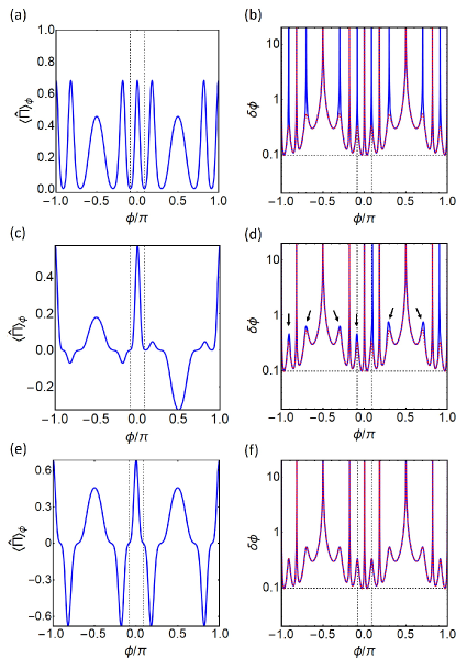
Figure 3: Output signal $\langle\hat{\Pi}\rangle_{\phi}$ and phase sensitivity $\delta\phi$ for $\mu_{-}=0$ and different choices of $\{\mu_{k}\}$. The parameters: $\bar{n}=200$, $a=1/2$, $b=3.8$, and $k_{f}=2$. (a) and (b): $\mu_{k}=1$ for all $k$’s. (c) and (d): $\{\mu_{-2},\mu_{-1},\mu_{0},\mu_{1},\mu_{2}\}=\{-0.715,0.068,0.839,-0.102,0.392\}$. (e) and (f): $\{\mu_{-2},\mu_{-1},\mu_{0},\mu_{1},\mu_{2}\}=\{1,-1,1,-1,1\}$. The red dashed lines: the CRB $1/\sqrt{F(\phi)}$. The vertical lines: locations of the first dark points $\phi_{\mathrm{dark}}\approx\pm b/\sqrt{\bar{n}}$. The horizontal lines in right panel: the best sensitivity $\delta\phi_{\min}\approx 1.37/\sqrt{\bar{n}}$.

For a general multi-outcome measurement, different choices of $\{\mu_{k}\}$ correspond to different observables $\hat{\Pi}=\sum_{k}\mu_{k}\hat{\Pi}_{k}$. Therefore, both the signal and the sensitivity depend on the eigenvalues $\{\mu_{k}\}$. To see it clearly, we take random numbers of $\{\mu_{k}\}$, ranged from $-1$ to $+1$. As shown by the blue solid lines of Figs. 3(c) and 3(d), one can see that both the signal and the sensitivity are different with that of Figs. 3(a) and  3(b). However, near $\phi=0$, the sensitivity in Fig. 3(d) coincides with that of Fig. 3(b), indicating that Eq. (21) still works to predict the best sensitivity. Remarkably, one can also see that the sensitivity does not diverge at the locations of the arrows. The singularity of $\delta\phi$ can be further suppressed using alternating signs of $\{\mu_{k}\}$ for neighbour outcomes (i.e., $\mu_{k\pm 1}=-\mu_{k}$). As shown in Figs. 3(e) and 3(f), one can see $\delta\phi\approx\delta\phi_{\mathrm{CRB}}=1/\sqrt{F(\phi)}$ within the whole phase interval. In other words, the inversion estimator associated with the so-chosen observable almost saturates the CRB.

We now adopt Monte Carlo method to simulate the above multi-outcome measurement Pezze ; Jin . Specially, we first generate $\mathcal{N}$ random numbers $\{\xi_{1},\xi_{2},...,\xi_{\mathcal{N}}\}$, according to the occurrence probabilities $\{P(k|\phi)\}$ at a given $\phi$, where $\xi_{i}$ (for $i=1$, $2$, $\cdots$, $\mathcal{N}$) can be regarded as the outcome $k=-k_{f}$, provided $0\leq\xi_{i}\leq P(-k_{f}|\phi)$. It can be regarded as the outcome $k=-k_{f}+1$, provided $P(-k_{f}|\phi)<\xi_{i}\leq P(-k_{f}|\phi)+P(-k_{f}+1|\phi)$, and so on. If $\xi_{i}$ obeys $P(-k_{f}|\phi)+P(-k_{f}+1|\phi)+\cdots+P(k_{f}|\phi)<\xi_{i}\leq 1$, then we treat it as the outcome “$-$”. In this way, we obtain the occurrence numbers of all the outcomes $\{\mathcal{N}_{k}\}$. Next, we repeat the above process for any value of $\phi\in(-\pi,\pi)$ and obtain the occurrence frequencies $\{\mathcal{N}_{k}/\mathcal{N}\}$. As depicted by Fig. 2, we show the averaged $\mathcal{N}_{k}/\mathcal{N}$ (the solid circles) and its standard deviation (the bars) after $M=10$ replicas of the above simulations. With large enough $\mathcal{N}$ ($=200$), one can see that the averaged occurrence frequency of each outcome almost follows its theoretical result, as is expected. Using Eqs. (3) and (19), we further obtain the average signal and its standard deviation. In Fig. 4(a), we take $\bar{n}=\alpha_{0}^{2}=1000$ and $b=3.2$, which gives $k_{f}=5$ and hence the number of outcomes $12$. Similar to Figs. 3(e) and (f), we choose alternating signs of the eigenvalues $\{\mu_{k}\}$ and vanishing $\mu_{-}$.

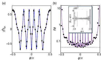
Figure 4: Output signal $\langle\hat{\Pi}\rangle_{\phi}$ and phase sensitivity $\delta\phi$ for alternating signs of $\{\mu_{k}\}$ and the parameters: $\bar{n}=1000$, $a=1/2$, $b=3.2$, and $k_{f}=5$ (i.e., total number of the outcomes is $12$). Solid circles: the averaged signal and the phase uncertainty of the inversion estimator $\phi_{\mathrm{inv}}$ obtained with ${\mathcal{N}}=200$ and $M=400$. The horizontal line in (b): the best sensitivity $\delta\phi_{\min}\approx 1.37/\sqrt{\bar{n}}$. Inset: Difference between the average value of the inversion estimator $\bar{\phi}_{\mathrm{inv}}=\sum_{i=1}^{M}\phi_{\mathrm{inv}}^{(i)}/M$ and the true value of phase shift $\phi$. The bars are the standard deviations of the estimators $\{\phi_{\mathrm{inv}}^{(1)},\phi_{\mathrm{inv}}^{(2)},...,\phi_{\mathrm{inv}}^{(M)}\}$.

In real experiments, the dependence of $P(k|\phi)$ on $\phi$ is obtained from replicas of $\mathcal{N}$ independent measurements at each given phase shift. This comprises a calibration of the interferometer. With all known occurrence probabilities and the signal, one can infer unknown value of $\phi$ via the phase estimation. As the simplest protocol, we adopt the inversion phase estimator $\phi_{\mathrm{inv}}=g^{-1}(\sum_{k}\mu_{k}{\mathcal{N}_{k}}/{\mathcal{N}})$, where $g^{-1}$ is the inverse function of the average signal $g(\phi)=\langle\hat{\Pi}\rangle_{\phi}$ and ${\mathcal{N}_{k}}/{\mathcal{N}}$ is the occurrence frequency of the $k$th outcome in a single $\mathcal{N}$ independent measurements. After $M$ replicas, one can obtain the estimators $\{\phi_{\mathrm{inv}}^{(1)},\phi_{\mathrm{inv}}^{(2)},...,\phi_{\mathrm{inv}}^{(M)}\}$. The mean value of the estimators $\bar{\phi}_{\mathrm{inv}}=\langle\phi_{\mathrm{inv}}^{(i)}\rangle_{s}$ and its standard deviation are shown in the inset of Fig. 4(b), where the statistical average is defined as $\langle(\cdots)\rangle_{s}\equiv\sum_{i=1}^{M}(\cdots)/M$. The standard deviation (the bars) is larger than $(\bar{\phi}_{\mathrm{inv}}-\phi)$ indicates that the inversion estimator is unbiased; see the inset of Fig. 4(b). For an effective single-shot measurement, the phase uncertainty is defined by $\sigma=\sqrt{{\mathcal{N}}}\sqrt{\langle(\phi_{\mathrm{inv}}^{(i)}-\phi)^{2}\rangle_{s}}$, which almost follows the lower bound of phase sensitivity $\delta\phi_{\mathrm{CRB}}=1/\sqrt{F(\phi)}$; see the solid circles of Fig. 4(b).

Finally, it should be mentioned that we have discussed the achievable sensitivity close to the shot-noise limit with the coherent-state input. However, it is possible to surpass this classical limit once the interferometer is fed by nonclassical states of light. Recently, Schäfermeier et al Schafermeier have demonstrated that both the resolution and the sensitivity can surpass their classical limits using the binary-outcome homodyne detection, where a coherent state and a squeezed vacuum are used as the input. For any binary-outcome measurement, we have shown that the phase estimator by inverting the average signal is good enough to saturate the CRB Feng ; Paris ; Jin . For a multi-outcome detection, the inversion estimator is less optimal due to the divergence of the phase sensitivity YMK ; Pezze . We show here that the singularity can be suppressed when the signal is a sum of positive $P(k|\phi)$, weighted by alternating signs of eigenvalues.

V Conclusion

In summary, we have considered quantum phase estimation with multi-outcome homodyne detection in the coherent-state light Mach-Zehnder interferometer. Compared with the ultimate phase sensitivity determined by the classical Fisher information, we show that (i) the phase sensitivity shows a series of extra divergences at the minima of the output signal; (ii) these extra divergences can be removed by using observables whose eigenvalues associated with neighboring outcomes have alternating signs. This result provides a family of nearly optimal inversion estimators that almost saturate the Cramér-Rao bound over the whole range of phases. We further perform numerical simulations using such observables and demonstrate that phase uncertainty of the inversion estimator almost follows the Cramér-Rao bound. Our method for removing extra divergences of the phase sensitivity may also be applicable to other kinds of multi-outcome measurements.

Funding

Science Foundation of Zhejiang Sci-Tech University (18062145-Y); National Natural Science Foundation of China (NSFC) (91636108, 11775190, and 11774021); the NSFC program for “Scientific Research Center” (U1530401).

References

- (1) M. Born and E. Wolf, Principle of Optics (Cambridge University, 1999)
- (2) C. M. Caves, “Quantum-mechanical noise in an interferometer,” Phys. Rev. D 23, 1693 (1981).
- (3) D. J. Wineland, J. J. Bollinger, W. M. Itano, and D. J. Heinzen, “Squeezed atomic states and projection noise in spectroscopy,” Phys. Rev. A. 50, 67 (1994).
- (4) D. Leibfried, M. D. Barrett, T. Schaetz, J. Britton, J. Chiaverini, W. M. Itano, J. D. Jost, C. Langer, and D. J. Wineland, “Toward Heisenberg-Limited Spectroscopy with Multiparticle Entangled States,” Science 304, 1476-1478 (2004).
- (5) J. P. Dowling, “Quantum optical metrology-the lowdown on high-N00N states,” Contemp. Phys. 49, 125-143 (2008).
- (6) A. N. Boto, P. Kok, D. S. Abrams, S. L. Braunstein, C. P. Williams, and J. P. Dowling, “Quantum Interferometric Optical Lithography: Exploiting Entanglement to Beat the Diffraction Limit,” Phys. Rev. Lett. 85, 2733 (2000).
- (7) M. W. Mitchell, J. S. Lundeen, and A. M. Steinberg, “Super-resolving phase measurements with a multiphoton entangled state,” Nature 429, 161-164 (2004).
- (8) P. Walther, J. W. Pan, M. Aspelmeyer, R. Ursin, S. Gasparoni, and A. Zeilinger, “de Broglie wavelength of a non-local four-photon state,” Nature 429, 158-161 (2004).
- (9) Y. A. Chen, X. H. Bao, Z. S. Yuan, S. Chen, B. Zhao, and J. W. Pan, “Heralded Generation of an Atomic NOON State,” Phys. Rev. Lett. 104, 043601 (2010).
- (10) I. Afek, O. Ambar, and Y. Silberberg, “High-NOON States by Mixing Quantum and Classical Ligh,” Science 328, 879-881 (2010).
- (11) D. Braun, G. Adesso, F. Benatti, R. Floreanini, U. Marzolino, M. W. Mitchell, and S. Pirandola, “Quantum-enhanced measurements without entanglement,” Rev. Mod. Phys. 90, 035006 (2018).
- (12) U. Dorner, R. Demkowicz-Dobrzanski, B. J. Smith, J. S. Lundeen, W. Wasilewski, K. Banaszek, and I. A. Walmsley, “Optimal Quantum Phase Estimation,” Phys. Rev. Lett. 102, 040403 (2009).
- (13) Y. M. Zhang, X. W. Li, W. Yang, and G. R. Jin, “Quantum Fisher information of entangled coherent states in the presence of photon loss,” Phys. Rev. A 88, 043832 (2013).
- (14) K. J. Resch, K. L. Pregnell, R. Prevedel, A. Gilchrist, G. J. Pryde, J. L. O’Brien, and A. G. White, “Time-Reversal and Super-Resolving Phase Measurements,” Phys. Rev. Lett. 98, 223601 (2007).
- (15) Y. Gao, P. M. Anisimov, C. F. Wildfeuer, J. Luine, H. Lee, and J. P. Dowling, “Super-resolution at the shot-noise limit with coherent states and photon-number-resolving detectors,” J. Opt. Soc. Am. B 27, A170-A174 (2010).
- (16) L. Cohen, D. Istrati, L. Dovrat, and H. S. Eisenberg, “Super-resolved phase measurements at the shot noise limit by parity measurement,” Opt. Express 22, 11945-11953 (2014).
- (17) E. Distante, M. Ježek, and U. L. Andersen, “Deterministic Superresolution with Coherent States at the Shot Noise Limit,” Phys. Rev. Lett. 111, 033603 (2013).
- (18) P. R. Bevington, Data Reduction and Error Analysis for the Physical Sciences (McGraw-Hill, 1969).
- (19) C. W. Helstrom, Quantum Detection and Estimation Theory (Academic, 1976).
- (20) S. L. Braunstein and C. M. Caves, “Statistical distance and the geometry of quantum states,” Phys. Rev. Lett. 72, 3439 (1994).
- (21) S. L. Braunstein, C. M. Caves, and G. J. Milburn, “Generalized Uncertainty Relations: Theory, Examples, and Lorentz Invariance,” Ann. Phys. (N.Y.) 247, 135-173 (1996).
- (22) M. G. A. Paris, “Quantum estimation for quantum technology,” Int. J. Quantum. Inform. 7, 125-137 (2009).
- (23) B. Yurke, S. L. McCall, and J. R. Klauder, “SU(2) and SU(1,1) interferometers,” Phys. Rev. A 33, 4033 (1986).
- (24) L. Pezzé, A. Smerzi, G. Khoury, J. F. Hodelin, and D. Bouwmeester, “Phase Detection at the Quantum Limit with Multiphoton Mach-Zehnder Interferometry,” Phys. Rev. Lett. 99, 223602 (2007).
- (25) J. J. Bollinger, W. M. Itano, D. J. Wineland, and D. J. Heinzen, “Optimal frequency measurements with maximally correlated states,” Phys. Rev. A 54, R4649 (1996).
- (26) C. C. Gerry, “Heisenberg-limit interferometry with four-wave mixers operating in a nonlinear regime,” Phys. Rev. A 61, 043811 (2000).
- (27) C. C. Gerry, A. Benmoussa, and R. A. Campos, “Nonlinear interferometer as a resource for maximally entangled photonic states: Application to interferometry,” Phys. Rev. A 66, 013804 (2002).
- (28) C.C. Gerry and J. Mimih, “The parity operator in quantum optical metrology,” Contemp. Phys. 51, 497-511 (2010).
- (29) P. M. Anisimov, G. M. Raterman, A. Chiruvelli, W. N. Plick, S. D. Huver, H. Lee, and J. P. Dowling, “Quantum Metrology with Two-Mode Squeezed Vacuum: Parity Detection Beats the Heisenberg Limit,” Phys. Rev. Lett. 104, 103602 (2010).
- (30) A. Chiruvelli and H. Lee, “Parity measurements in quantum optical metrology,” J. Mod. Opt. 58, 945-953 (2011).
- (31) K. P. Seshadreesan, S. Kim, J. P. Dowling, and H. Lee, “Phase estimation at the quantum Cram-Rao bound via parity detection,” Phys. Rev. A 87, 043833 (2013).
- (32) X. M. Feng, G. R. Jin, and W. Yang, “Quantum interferometry with binary-outcome measurements in the presence of phase diffusion,” Phys. Rev. A. 90, 013807 (2014).
- (33) L. Ghirardi, I. Siloi, P. Bordone, F. Troiani, and M. G. A. Paris, “Quantum metrology at level anticrossing,” Phys. Rev. A 97, 012120 (2018).
- (34) G. R. Jin, W. Yang, and C. P. Sun, “Quantum-enhanced microscopy with binary-outcome photon counting,” Phys. Rev. A 95, 013835 (2017).
- (35) J. D. Zhang, Z. J. Zhang, L. Z. Cen, J. Y. Hu, and Y. Zhao, “Deterministic super-resolved estimation towards angular displacements based upon a Sagnac interferometer and parity measurement,” arXiv:1809.04830 (2018).
- (36) J. D. Zhang, Z. J. Zhang, L. Z. Cen, S. Li, Y. Zhao, and F. Wang, “Super-resolution and super-sensitivity of entangled squeezed vacuum state using optimal detection strategy,” Chin. Phys. B 26, 094204 (2017).
- (37) Z. J. Zhang, T. Y. Qiao, L. Z. Cen, J. D. Zhang, F. Wang, and Y. Zhao, “Optimal quantum detection strategy for super-resolving angular-rotation measurement,” Appl. Phys. B 123, 148 (2017).
- (38) Q. Wang, L. L. Hao, H. X. Tang, Y. Zhang, C. H. Yang, X. Yang, L. Xu, and Y. Zhao, “Super-resolving quantum LiDAR with even coherent states sources in the presence of loss and noise,” Phys. Lett. A 380, 3717 (2016).
- (39) Q. Wang, L. L. Hao, Y. Zhang, L. Xu, C. H. Yang, X. Yang, and Y. Zhao, “Super-resolving quantum lidar: entangled coherent-state sources with binary-outcome photon counting measurement suffice to beat the shot-noise limit,” Opt. Express 24, 5045-5056 (2016).
- (40) C. C. Gerry and P. L. Knight, Introductory Quantum Optics (Cambridge University, 2005).
- (41) K. P. Seshadreesan, P. M. Anisimov, H. Lee, and J. P. Dowling, “Parity detection achieves the Heisenberg limit in interferometry with coherent mixed with squeezed vacuum light,” New J. Phys. 13, 083026 (2011).
- (42) Q. S. Tan, J. Q. Liao, X. G. Wang, and F. Nori, “Enhanced interferometry using squeezed thermal states and even or odd states,” Phys. Rev. A 89, 053822 (2014).
- (43) C. Schafermeier, M. Jezex, L. S. Madsen, T. Gehring, and U. L. Andersen, “Deterministic phase measurements exhibiting super-sensitivity and super-resolution,” Optica 5, 60-64 (2018).