Adversarial-Residual-Coarse-Graining: Applying machine learning theory to systematic molecular coarse-graining

Abstract

We utilize connections between molecular coarse-graining approaches and implicit generative models in machine learning to describe a new framework for systematic molecular coarse-graining (CG). Focus is placed on the formalism encompassing generative adversarial networks. The resulting method enables a variety of model parameterization strategies, some of which show similarity to previous CG methods. We demonstrate that the resulting framework can rigorously parameterize CG models containing CG sites with no prescribed connection to the reference atomistic system (termed virtual sites); however, this advantage is offset by the lack of a closed-form expression for the CG Hamiltonian at the resolution obtained after integration over the virtual CG sites. Computational examples are provided for cases in which these methods ideally return identical parameters as Relative Entropy Minimization (REM) CG but where traditional REM CG optimization equations are not applicable.

I Introduction

Classical atomistic molecular dynamics (MD) simulation has provided significant insight into many biological and materials processes.Karplus and McCammon (2002); Marx and Hutter (2009); Dror et al. (2012); Karplus and Lavery (2014) However, its efficacy is often restricted by its computational cost: for example, routine atomic resolution studies of biomolecular systems are currently limited to microsecond simulations of millions of atoms. Phenomena that cannot be characterized in this regime often require investigation using modified computational approaches. Coarse-grained (CG) molecular dynamics can be effective for studying systems where the motions of nearby atoms are highly interdependent.Voth (2008); Saunders and Voth (2013); Noid (2013); Brini et al. (2013); Baaden and Marrink (2013) By simulating at the resolution of CG sites or “beads”, each associated with multiple correlated atoms, biomolecular processes at the second timescale and beyond can be accurately probed. High-fidelity CGMD models often depend on flexible parameterizations; as a result, the design of systematic parameterization strategies is an active area of study (e.g., methods and applications in references 10; 11; 12; 13; 14; 15; 16; 17; 18; 19; 20; 21; 22; 23; 24; 25; 26; 27; 28; 29; 30; 31; 32).

The CGMD models considered in this article are similar to their atomistic counterparts. They are composed of point-mass CG beads, a corresponding CG force-field, and a simulation protocol that produces Boltzmann statistics in the long-time limit. We restrict the bulk of our study to the parameterization of the CG effective force-field. Here, and in the remainder of the article, we refer to these models simply as CG models. We only consider the static equilibrium properties of these models, and not their dynamics. There are two nonexclusive classes of parameterization strategies for CG models of interest to this article: top-down and bottom-up approaches.Voth (2008); Noid (2013); Saunders and Voth (2013) Top-down approaches aim to parameterize CG models to recapitulate specific macroscopic properties, such as pressure and partition coefficients, while bottom-up methods attempt to parameterize CG models to reproduce the multidimensional distribution given by explicitly mapping each atomistic configuration (produced by a suitable reference simulation) to a specific CG configuration.Izvekov and Voth (2005); Noid et al. (2007); Shell (2008); Noid et al. (2008a, b) The distribution of this mapped system is produced via a Boltzmann distribution with respect to an effective CG Hamiltonian referred to as the many-body Potential of Mean Force (PMF).

Certain scientific inferences could be informally drawn from the fit CG force-field itself, assuming that the force-field is constrained to intuitive low dimensional contributions (e.g., pairwise forces, such as in ref 34). For example, one could attempt to infer the effect of an amino acid mutation on protein behavior by considering how the approximated PMF differs when fit on reference wild type and mutant proteins simulations, similar to the analysis of low dimensional free energy surfaces. However, the primary use of CG models is typically based on their ability to generate CG configurations of a system of interest using their approximate force-field. Srivastava and Voth (2012); Cao et al. (2012); Dunn and Noid (2016); Carmichael and Shell (2012) The computational similarity of CG models with their atomistic counterparts allows CG models to be simulated using the same high performance software packages as those used in atomistic simulation.Plimpton (1995); Abraham et al. (2015); Brooks et al. (1983); Anderson, Lorenz, and Travesset (2008); Case et al. (2005); Phillips et al. (2005); Bowers et al. (2006) As a result, the computational profile of CG models is often controlled by the same dominating factor as atomistic models: the calculation of the force-field at each timestep.Plimpton (1995); Plimpton and Thompson (2012); Markidis and Laure (2015) This cost provides additional motivation for specific low dimensional force-field contributions. However, there is no guarantee that a force-field characterized solely by traditional bonded and pairwise nonbonded terms either describes the true PMF of the CG variables or can accurately reproduce all observables of interest to the parameterization.Voth (2008); Noid (2013); Saunders and Voth (2013) In the case of bottom-up methods, while typical approaches will produce the PMF in the infinite sampling limit when they are capable of representing any CG force-field, in practice each method creates a characteristic approximation (e.g., reproducing two-body at the expense of higher order correlations).

The compromises invoked by various bottom-up CG methods in realistic applications are critical to the utility of the resulting models. Certain methods focus on reproducing correlations dual to the potential form used;Rudzinski and Noid (2011); Lyubartsev and Laaksonen (1995); Chaimovich and Shell (2011); Reith, Pütz, and Müller-Plathe (2003) for example, when using a pairwise nonbonded potential these methods recapitulate the radial distribution function of the target system. Other specific methods are characterized by attempting to reproduce both these dual correlations along with certain higher order correlations intrinsically connected to the CG potential.Noid et al. (2007, 2008a); Mullinax and Noid (2009); Rudzinski and Noid (2011); Izvekov and Voth (2005); Mullinax and Noid (2009); Noid et al. (2007) The nature of the distributions approximated suggests three natural approaches for improving an inaccurate model: improve the CG force-field basis used, modify the CG representation, or select a different procedure to generate the CG force-field. The first two options are often a central part of the design of a systematic CG model; however, realistic systems, such as proteins, may not be well described by correlations that are typically connected to computationally efficient CG potentials coupled with appropriate CG representations.Noid (2013) More generally, the specific correlations critical to a reasonably accurate CG model may depend on the study at hand, and may be representable by simple force-fields—but only at the expense of other correlations connected to that potential form as dictated by a particular method. As a result, the diversity of possible applications motivates the creation of additional strategies for bottom-up CG modeling, each of which has different biases in the approximations it produces.

The task of generating examples (such as images) similar to a known empirical sample is of significant interest to the Machine Learning (ML) community.Goodfellow (2016); Doersch (2016); Alain et al. (2016); Mohamed and Lakshminarayanan (2016) The creation of an artificial process that can produce realistic samples often entails encoding an understanding of the true mechanism underlying the real world distribution; internal representations of an accurately parameterized generative model, such as neural network parameters, can be transferred for use in secondary tasks such as classificationRadford, Metz, and Chintala (2015) or image retrieval.Creswell and Bharath (2016) The artificial samples produced by the models themselves have additionally shown value by providing novel molecular targets for synthesis Sanchez-Lengeling et al. (2017); Ertl et al. (2017) or as labeled images for training in classification or regression.Shafaei, Little, and Schmidt (2016); Wood et al. (2016) A substantial number of these complex applications utilize implicit generative models. Mohamed and Lakshminarayanan (2016); Goodfellow et al. (2014); Salakhutdinov and Larochelle (2010); Kingma and Welling (2013) Implicit generative models, such as Generative Adversarial Networks (GANs),Goodfellow et al. (2014) are characterized by their lack of an explicit probability distribution, or an associated free energy, at the resolution they produce examples.Mohamed and Lakshminarayanan (2016) For example, a GAN may be trained to generate pictures containing human faces.Goodfellow et al. (2014) Each picture that could be generated has a parameterization specific probability of being a reasonable picture of a human face (admittedly, this probability is often very close to one or zero); however, the GAN itself does not have explicit knowledge of this probability. Instead, the GAN is simply characterized as a procedure that transforms random numbers from a simple noise distribution to images that follow the probability distribution of plausible images. The methods used to parameterize (i.e., train) GANs therefore focus on the ability to critique a model distribution against reference samples without knowledge of the probability density function characterizing the model. This is in strong contrast to typical molecular simulation, Karplus and McCammon (2002); Frenkel and Smit (2002); Allen and Tildesley (2017) which traditionally requires a known free energy surface to produce samples through molecular dynamics or Markov Chain Monte Carlo—and whose systematic parameterization techniques often naturally explicitly involve evaluation of the corresponding model free energy surface. Stillinger (1970); Lyubartsev and Laaksonen (1995); Izvekov and Voth (2005); Noid et al. (2007, 2008a, 2008b); Shell (2008); Mullinax and Noid (2009); Karimi-Varzaneh et al. (2011); Carmichael and Shell (2012); Dama et al. (2013); Rudzinski and Noid (2015); Lyubartsev et al. (2015); Vlcek and Chialvo (2015); de Oliveira et al. (2016); Sanyal and Shell (2016); Dunn and Noid (2016); Lemke and Peter (2017); John and Csanyi (2017); Wagner et al. (2017); Tsourtis, Harmandaris, and Tsagkarogiannis (2017); Zhang et al. (2013) However, both methods are focused on accurately producing samples, or configurations, as their primary goal.

This article focuses on making this intuitive connection between GANs and molecular models explicit, allowing us to apply established insight from the adversarial community to bottom-up CG modeling, giving rise to new strategies for CG parameterization we term Adversarial-Residual-Coarse-Graining (ARCG). By doing so we facilitate the use of additional classes of CG model quality measures that may show promise in modifying the approximations characterizing the optimal CG model when using a constrained set of candidate potentials to represent the CG force-field. We additionally find that it is possible to decouple the resolution at which one critiques the behavior of the CG model and the resolution at which a CG force-field is required: as an example we describe a novel rigorous avenue to increase the expressiveness of bottom-up CG models through the use of virtual sites. Critically, we do not utilize a full GAN architecture to generate CG samples; rather, we utilize the supporting theory Goodfellow et al. (2014); Reid and Williamson (2011); Nowozin, Cseke, and Tomioka (2016); Nguyen, Wainwright, and Jordan (2010); Bouchacourt, Mudigonda, and Nowozin (2016); Bottou et al. (2017); Arjovsky, Chintala, and Bottou (2017) to optimize traditional CG force-fields.

In this work we discuss formal connections between CG and GAN-type implicit generative models and provide an initial implementation of the resulting ARCG framework. Section II provides both an informal and a formal summary of the theoretical underpinnings, while section III provides details on a particular instance of ARCG and a public computational implementation. Section IV then provides results on three simple test systems, and section V outlines the consequences of the results and possible future studies. Section VI provides concluding remarks.

II Theory

The purpose of this section is to both informally describe and formally define ARCG, and to summarize connections between ARCG and previous CG parameterization methods. We begin by presenting an intuitive understanding of a specific form of ARCG to provide clarity for the subsequent mathematical description. We then follow by defining notation and the fine-grained/CG systems to which ARCG applies. We define ARCG and describe its estimation and optimization. We then move to decouple the resolution at which one critiques the CG model from the resolution native to the CG Hamiltonian, thereby generalizing our application to systems containing virtual CG sites. We continue by discussing the corresponding challenges with momentum consistency, and we finish by summarizing ARCG’s relationship to previous CG methods.

II.1 Informal Description of ARCG

Bottom-up CG models are parameterized to approximate the free energy surface implied by mapping fine-grained (FG) configurations to the CG resolution.Noid (2013); Saunders and Voth (2013) Generally, this entails considering many different possible CG models (each, for example, characterized by a different pair potential) and their relationship to the reference FG data. Often, this is operationalized by creating a variational statement and searching for the CG model that minimizes it (for example, minimizing the relative entropy between the CG model and FG dataShell (2008)). After such a procedure is complete the modeler is well advised to visually inspect and compare the configurations produced by the selected CG model to those produced by the reference FG model. If the configurations are dissimilar, then the CG model is likely not adequate, and aspects of the variational statement or set of initial models considered must be modified and the parameterization process repeated.

It is natural to ask whether the final inspection of configurations produced by the FG and CG models can be intrinsically linked to the variational statement parameterizing the CG model. It is intuitive that for systematic CG parameterization methods derived from configurational consistency Stillinger (1970); Lyubartsev and Laaksonen (1995); Izvekov and Voth (2005); Noid et al. (2007, 2008a, 2008b); Shell (2008); Mullinax and Noid (2009); Karimi-Varzaneh et al. (2011); Carmichael and Shell (2012); Dama et al. (2013); Rudzinski and Noid (2015); Lyubartsev et al. (2015); Vlcek and Chialvo (2015) that when an indefinite amount of samples are used and all possible CG models are considered that the optimized CG model will perfectly reproduce the mapped FG statistics, and as a result, the configurations produced by the FG and CG models will be indistinguishable. However, in cases where perfectly reproducing the FG statistics is infeasible it seems natural to ask if a model could be trained using this criteria of distinguishability directly.

While it could be possible in simple situations to use a human observer to intuitively rank CG models by considering the configurations they produce, this procedure quickly becomes subjective and untenable for complex models. A natural progression in method design is then to train a computer to distinguish CG models by comparing their samples against the reference data set. One appropriate statistical procedure is classification,James et al. (2013) where a computer attempts to differentiate individual configurations based on whether they are more likely drawn from either the CG or mapped FG data sets. The implied procedure for CG parameterization is then to optimize the CG model such that it is intrinsically difficult to complete this task: as a result, the computer will inevitably make many mistakes on average when attempting to isolate configurations characteristic to only the FG and CG data. One possible intuitive manifestation of ARCG theory concretely implements this classification procedure while maintaining clear connection to CG methods such as relative entropy minimization (REM).Shell (2008) Previous CG parameterization methods have used similar, but not identical, motivations to produce parameterization strategies.Lemke and Peter (2017); Vlcek and Chialvo (2015); Shell (2008) ARCG theory serves to connect, clarify, and reframe these methods where possible while extending beyond the classification metaphor.

It is important to note that the task of classification is a variational procedure itself:James et al. (2013); Reid and Williamson (2011) the ideal estimate of the true sources of a set of molecular configurations has a lower error than all other estimates. The optimization in classification searches over these various possible hypotheses. As a result, at each step of force-field optimization ARCG must perform this variational search over possible hypotheses, resulting in two nested variational statements in the full model optimization procedure: one required for classification, and the other for choosing the resulting CG model. Importantly, the error rate of the optimal classifier can be explicitly linked to various $f$-divergences (e.g., relative entropy) evaluated between the mapped FG and CG distributions.Reid and Williamson (2011) This suggests an equivalent formalism with which to view ARCG: the variational estimation of divergences. This alternate interpretation additionally illustrates how additional divergences, such as the Wasserstein distance,Arjovsky, Chintala, and Bottou (2017) can be estimated, even without a clear connection to classification. As a result, ARCG theory is primarily treated through the lens of variational divergence estimation in the following sections.

The variational estimation intrinsic to ARCG affords an interesting extension to traditional parameterization strategies: the resolution at which the CG Hamiltonian acts may be finer than the resolution at which the model is compared to the reference data. Equivalently, CG samples can be mapped before being compared to the mapped reference FG samples. For example, additional particles may be introduced to facilitate complex effective interactions between the CG particles, and then may be mapped out before comparing to the mapped reference FG samples. Applying such a mapping creates issues with many other parameterization strategies as discussed in section II.6.

II.2 Model Definitions and Selection

We consider a FG probability density ${p^{\text{FG}}_{\text{ref}}}$ and a mapping operator $\mathpzc{M}$ that maps a FG configuration to a CG configuration. The FG simulation is constructed such that it produces samples from the Boltzmann distribution with respect to a FG Hamiltonian giving the following probability density:

$${p^{\text{FG}}_{\text{ref}}}(\mathbf{r}^{3n},\mathbf{p}^{3n}):={Z^{\text{FG}}_{\text{ref},\mathbf{r}}}^{-1}{Z^{\text{FG}}_{\text{ref},\mathbf{p}}}^{-1}\exp\left[-\beta\left(\sum_{i=1}^{n}\frac{\mathbf{p}_{i}^{2}}{2m_{i}}+{U^{\text{FG}}_{\text{ref}}}(\mathbf{r}^{3n})\right)\right]={p^{\text{FG}}_{\text{ref},\mathbf{p}}}(\mathbf{p}^{3n}){p^{\text{FG}}_{\text{ref},\mathbf{r}}}(\mathbf{r}^{3n})$$ (1)

where $\beta$ is $\frac{1}{\textrm{k}_{b}T}$ with the temperature $T$ set by the simulation protocol, $m_{i}$ are the FG masses, $\mathbf{r}^{3n}$ and $\mathbf{p}^{3n}$ are the FG positions and momenta variables, and our partition functions are defined as expected such that

$${Z^{\text{FG}}_{\text{ref},\mathbf{r}}} = \int_{{\mathcal{X}^{\text{FG}}_{\mathbf{r}}}}\exp\left[-\beta{U^{\text{FG}}_{\text{ref}}}(\mathbf{r}^{3n})\right]\mathrm{d}\mathbf{r}^{3n}$$ (2)

$${Z^{\text{FG}}_{\text{ref},\mathbf{p}}} = \int_{{\mathcal{X}^{\text{FG}}_{\mathbf{p}}}}\exp\left[-\beta\sum_{i=1}^{n}\frac{\mathbf{p}_{i}^{2}}{2m_{i}}\right]\mathrm{d}\mathbf{p}^{3n}$$ (3)

where the integrals are taken over the full domains of the position and momentum variables (denoted via ${\mathcal{X}^{\text{FG}}_{\mathbf{r}}}$ and ${\mathcal{X}^{\text{FG}}_{\mathbf{p}}}$). The application of the CG map $\mathpzc{M}$ produces CG configurations that follow an implied probability distribution. $\mathpzc{M}$ is constrained such that it is linear and can be decomposed into momentum and position components, i.e., $\mathpzc{M}(\mathbf{r}^{3n},\mathbf{p}^{3n})=[{\mathpzc{M}_{\mathbf{r}}}(\mathbf{r}^{3n});{\mathpzc{M}_{\mathbf{p}}}(\mathbf{p}^{3n})]$, implying a factorizable probability density ${p_{\text{ref}}}(\mathbf{R}^{3N},\mathbf{P}^{3N}):={p_{\text{ref},\mathbf{R}}}(\mathbf{R}^{3N}){p_{\text{ref},\mathbf{P}}}(\mathbf{P}^{3N})$ over the CG variables defined as

$${p_{\text{ref},\mathbf{R}}}(\mathbf{R}^{3N}) := \int_{{\mathcal{X}^{\text{FG}}_{\mathbf{r}}}}{p^{\text{FG}}_{\text{ref},\mathbf{r}}}(\mathbf{r}^{3n})\delta({\mathpzc{M}_{\mathbf{r}}}(\mathbf{r}^{3n})-\mathbf{R}^{3N})\mathrm{d}\mathbf{r}^{3n}$$ (4)

$${p_{\text{ref},\mathbf{P}}}(\mathbf{P}^{3N}) := \int_{{\mathcal{X}^{\text{FG}}_{\mathbf{p}}}}{p^{\text{FG}}_{\text{ref},\mathbf{p}}}(\mathbf{p}^{3n})\delta({\mathpzc{M}_{\mathbf{p}}}(\mathbf{p}^{3n})-\mathbf{P}^{3N})\mathrm{d}\mathbf{p}^{3n}.$$ (5)

Bottom-up CG models aim to directly produce samples from the distribution described by ${p_{\text{ref}}}$.Noid et al. (2007, 2008a) Ideally, this is achieved by defining a model CG Hamiltonian $\left(\sum_{i=1}^{N}\frac{\mathbf{P}_{i}^{2}}{2M_{i}}+{U_{\text{mod}}}(\mathbf{R}^{3N})\right)$ such that the corresponding Boltzmann statistics

$${p_{\text{mod}}}(\mathbf{R}^{3N},\mathbf{P}^{3N}):={Z_{\text{mod},\mathbf{R}}}^{-1}{Z_{\text{mod},\mathbf{P}}}^{-1}\exp\left[-\beta\left(\sum_{i=1}^{N}\frac{\mathbf{P}_{i}^{2}}{2M_{i}}+{U_{\text{mod}}}(\mathbf{R}^{3N})\right)\right]={p_{\text{mod},\mathbf{R}}}(\mathbf{R}^{3N}){p_{\text{mod},\mathbf{P}}}(\mathbf{P}^{3N})$$ (6)

are ideally identical to the mapped FG statistics, criteria expressed with the following CG consistency equations Noid et al. (2008a)

$${p_{\text{ref},\mathbf{R}}}(\mathbf{R}^{3N}) = {p_{\text{mod},\mathbf{R}}}(\mathbf{R}^{3N})$$ (7)

$${p_{\text{ref},\mathbf{P}}}(\mathbf{P}^{3N}) = {p_{\text{mod},\mathbf{P}}}(\mathbf{P}^{3N}).$$ (8)

Momentum and configurational consistency are generally treated separately, with momentum consistency exactly satisfied through direct definition of CG masses $M_{i}$ and configurational consistency approximated through a variational statement (as the corresponding integral is not generally tractable).Noid et al. (2008a) We defer further discussion of momentum consistency until subsection II.5.1. The configurational variational statement is specific to the particular bottom-up CG method chosen and utilizes a variety of information depending on the method considered. Generally, knowledge of ${U^{\text{FG}}_{\text{ref}}}$, ${U_{\text{ref}}}$, and $\mathpzc{M}$ are used. In many cases the corresponding variational principle can be considered in the following form

$${\boldsymbol{\theta}}^{\dagger}:=\operatorname*{arg\!\min}_{{\boldsymbol{\theta}}}\mathcal{F}[{p_{\text{mod},\mathbf{R},{\boldsymbol{\theta}}}},{p_{\text{ref},\mathbf{R}}}]$$ (9)

where ${\boldsymbol{\theta}}$ denotes the finite parameterization of our CG potential, ${\boldsymbol{\theta}}^{\dagger}$ parameterizes our ideal model, and $\mathcal{F}$ is a function characterizing the quality of our model. Often,Izvekov and Voth (2005); Shell (2008); Noid et al. (2007, 2008a, 2008b); Vlcek and Chialvo (2015); Stillinger (1970); Mullinax and Noid (2009) the exact form of the variational statement contains intractable integrals which are approximated via empirical averages from atomistic and coarse-grained trajectories.

Importantly, while the models discussed in the remainder of this article fit into this framework, they differ in one important respect to many previous CG parameterization strategies: they introduce a variational definition of $\mathcal{F}$ itself, resulting in two nested variational statements in the numerical optimization procedure.

II.3 Adversarial-Residual-Coarse-Grained Models

ARCG models are characterized by a set of possible $\mathcal{F}$ that are defined variationally as the difference in ensemble averages of a pair of coupled scalar functions. The functions, $f$ and $g$, are found as producing the maximum of the following variational definition

$$\mathcal{F}[{p_{\text{mod},\mathbf{R},{\boldsymbol{\theta}}}},{p_{\text{ref},\mathbf{R}}}]:=\max_{(f,g)\in\mathcal{Q}}\left\{\langle f\rangle_{p_{\text{mod},{\boldsymbol{\theta}}}}-\langle g\rangle_{p_{\text{ref}}}\right\},$$ (10)

leading to a minimax variational statement for the fit model itself

$${\boldsymbol{\theta}}^{\dagger}=\operatorname*{arg\!\min}_{\boldsymbol{\theta}}\left[\max_{(f,g)\in\mathcal{Q}}\left\{\langle f\rangle_{{p_{\text{mod},{\boldsymbol{\theta}}}}}-\langle g\rangle_{p_{\text{ref}}}\right\}\right].$$ (11)

In other words, for a specific choice of ${p_{\text{mod}}}$ and ${p_{\text{ref}}}$ the numerical value of our residual is determined by a specific $(f,g)$ pair; all other choices of pairs of observables in $\mathcal{Q}$ produce a more optimistic estimate of the quality of our model. These observables are evaluated via their configurational average at the CG resolution. As we update ${\boldsymbol{\theta}}$, the optimal choice of $(f,g)$ will change.

The definition of $\mathcal{Q}$ depends on the particular $\mathcal{F}$ being specified. For example, if $f=g$ for all pairs in $\mathcal{Q}$, this expression defines the class of Maximum Mean Discrepancy (MMD) distances,Gretton et al. (2012); Dziugaite, Roy, and Ghahramani (2015) with each MMD distance then being defined by further constraints on $\mathcal{Q}$. Typically, the function space in MMD is restricted to the unit ball in a reproducing kernel Hilbert space, a choice which allows the maximization to be resolved via a closed expression. The examples in this paper will estimate $f$-divergences: in this case,

$$\mathcal{Q}:=\left\{\left(-\frac{1}{2}l_{\text{mod}}\circ\hat{\eta},\frac{1}{2}l_{\text{mod}}\circ\hat{\eta}\right):\hat{\eta}\in[0,1]^{\mathcal{X}_{\mathbf{R}}}\right\}$$ (12)

where we have used $\circ$ to denote function compositions, e.g., $f\circ g(x):=f(g(x))$, $[0,1]^{\mathcal{X}_{\mathbf{R}}}$ denotes the set of functions from $\mathcal{X}_{\mathbf{R}}$ to $[0,1]$, and $l_{\text{ref}}$ and $l_{\text{mod}}$ are functions determined by the specific $f$-divergence estimated and whose closed form is given in the next section.

Model selection requires an optimization over ${\boldsymbol{\theta}}$ to satisfy the external minimization in Eq. (11). The strategies available for doing so depend on the structure of $\mathcal{Q}$. For low dimensional parameterizations, it may be feasible to do a grid search over possible models and to use Eq. (10) to select the ideal model. However, for higher dimensional parameter spaces an attractive option is to use methods utilizing the gradient with respect to ${\boldsymbol{\theta}}$. If the maximized estimate over $\mathcal{Q}$ is differentiable at a particular point with respect to ${\boldsymbol{\theta}}$, then (due to the envelope theoremMilgrom and Segal (2002), see Appendix A) the derivatives with respect to ${\boldsymbol{\theta}}$ at that point only include terms related to the ensemble average over the model distribution, ${p_{\text{mod}}}$

$$\frac{\mathrm{d}}{\mathrm{d}{\boldsymbol{\theta}}_{i}}\mathcal{F}[{p_{\text{mod},{\boldsymbol{\theta}}}},{p_{\text{ref}}}] = \frac{\mathrm{d}}{\mathrm{d}{\boldsymbol{\theta}}_{i}}\max_{(f,g)\in\mathcal{Q}}\left\{\langle f\rangle_{{p_{\text{mod},{\boldsymbol{\theta}}}}}-\langle g\rangle_{p_{\text{ref}}}\right\}\;\;\;$$ (13)

$$= \frac{\partial}{\partial{\boldsymbol{\theta}}_{i}}\langle f^{\dagger}\rangle_{{p_{\text{mod},{\boldsymbol{\theta}}}}}$$ (14)

where $f^{\dagger}$ represents one of the optimal observables found at the internal maximum. When the maximized inner estimate is expressible in closed form (which is true in the case of the $f$-divergences estimated in this paper), we can directly confirm the existence of this derivative. Assuming that the observable is regular enough such that the integral and derivative operators may be exchanged, simple substitution provides a covariance expression for estimation:

$$\frac{\partial}{\partial{\boldsymbol{\theta}}_{i}}\left\langle f^{\dagger}\right\rangle_{{p_{\text{mod},{\boldsymbol{\theta}}}}}=\beta\left\langle f^{\dagger}\right\rangle_{{p_{\text{mod},{\boldsymbol{\theta}}}}}\left\langle\frac{\partial U_{\boldsymbol{\theta}}}{\partial{\boldsymbol{\theta}}_{i}}\right\rangle_{{p_{\text{mod},{\boldsymbol{\theta}}}}}-\beta\left\langle f^{\dagger}\frac{\partial U_{\boldsymbol{\theta}}}{\partial{\boldsymbol{\theta}}_{i}}\right\rangle_{{p_{\text{mod},{\boldsymbol{\theta}}}}}.$$ (15)

These results suggest a straightforward numerical optimization of Eq. (11) using gradient descent and related first order methods (e.g., RMSpropHinton, Srivastava, and Swersky (2012)). We represent $\mathcal{Q}$ by indexing with a finite dimensional vector $\boldsymbol{\psi}$. At each iteration of optimization, holding ${\boldsymbol{\theta}}$ constant, we maximize over $\boldsymbol{\psi}$ using samples from the model and reference distributions to estimate our expected values; then, holding $\boldsymbol{\psi}$ constant, we take a single step on the gradient of ${\boldsymbol{\theta}}$ estimated by the sample average of the covariance expression. This two step process is completed until convergence of ${\boldsymbol{\theta}}$.

Not all definitions of $\mathcal{Q}$ produce meaningful procedures for creating CG models. Generally, particular forms of $\mathcal{F}$ are derived individually, each of which is amenable to the procedures outlined here. We continue by investigating an informative subset of possible $\mathcal{F}$, characterized via $f$-divergences, that will provide functionality directly encompassing REM CG,Shell (2008) as well as previous approaches by Stillinger (1970) and Vlcek and Chialvo (2015).

II.4 $f$-divergences

The $f$-divergences are a category of functions characterizing the difference between two distributions.Reid and Williamson (2011) When probability density functions are available we can express this family of divergences as

$$\mathbb{I}_{f}({p_{\text{ref}}},{p_{\text{mod}}}):=\int_{\chi}{p_{\text{mod}}}(x)f\left(\frac{{p_{\text{ref}}}(x)}{{p_{\text{mod}}}(x)}\right)\mathrm{d}x$$ (16)

where each member of the family is indexed by a convex function $f$ that satisfies $f(1)=0$. Relative entropy, the divergence central to REM CG, can be obtained by defining $f(x):=x\log x$, and the Hellinger distance, central to previous methods by Stillinger (1970) and Vlcek and Chialvo (2015) can be obtained by via $f(x):=\left(\sqrt{x}-1\right)^{2}$.

The $f$-divergence between ${p_{\text{mod}}}$ and ${p_{\text{ref}}}$ can be expressed in multiple variational statements.Reid and Williamson (2011); Nowozin, Cseke, and Tomioka (2016); Nguyen, Wainwright, and Jordan (2010); Bottou et al. (2017) We here utilize its duality with the difficulty of classification which is mathematically expressed in the following formulation, giving the form

$$\mathbb{I}_{f}({p_{\text{mod}}},{p_{\text{ref}}})=\max_{\hat{\eta}\in[0,1]^{\mathcal{X}_{\mathbf{R}}}}\left[-\frac{1}{2}\langle l_{\text{mod}}\circ\hat{\eta}\rangle_{p_{\text{mod}}}-\frac{1}{2}\langle l_{\text{ref}}\circ\hat{\eta}\rangle_{p_{\text{ref}}}\right]$$ (17)

where

$$\underline{L}(x) := -2(1-x)f\left(\frac{x}{1-x}\right)$$

$$l_{\text{mod}}(h) := \underline{L}(h)-h\left.\frac{\partial\underline{L}}{\partial x}\right\rvert_{h}$$

$$l_{\text{ref}}(h) := \underline{L}(h)+(1-h)\left.\frac{\partial\underline{L}}{\partial x}\right\rvert_{h}.$$

The function $\hat{\eta}$ is a function of a CG configuration, mapping each configuration to a real number in $[0,1]$. Note that substitution into Eq. (11) (along with the removal of prefactors) provides us with our training residual

$${\boldsymbol{\theta}}^{\dagger}=\operatorname*{arg\!\min}_{\boldsymbol{\theta}}\left[\max_{\hat{\eta}\in[0,1]^{\mathcal{X}_{\mathbf{R}}}}\left\{-\langle l_{\text{mod}}\circ\hat{\eta}\rangle_{{p_{\text{mod},{\boldsymbol{\theta}}}}}-\langle l_{\text{ref}}\circ\hat{\eta}\rangle_{p_{\text{ref}}}\right\}\right]$$ (18)

where the optimal $\hat{\eta}$ producing the corresponding $f$-divergence, denoted $\eta$, is known to beReid and Williamson (2011)

$$\eta(x)=\frac{{p_{\text{ref}}}(x)}{{p_{\text{mod}}}(x)+{p_{\text{ref}}}(x)}.$$ (19)

While here we have denoted our inner variational statement as optimizing over a space of functions instead of pairs of functions, this is equivalent to Eq. (11) when defining $\mathcal{Q}$ via Eq. $\eqref{pairspacelink}$. In the context of $f$-divergences, when $\mathcal{Q}$ contains $(-\frac{1}{2}l_{\text{mod}}\circ\eta,\frac{1}{2}l_{\text{mod}}\circ\eta)$, i.e. when optimization with the population averages would return the corresponding $f$-divergence, we will refer to that $\mathcal{Q}$ as being complete. Additionally, when $\mathcal{Q}$ is expressive enough such that it is complete for each step in an optimization process, we will additionally refer to it as complete, with the distinction evident from context. We provide concrete expressions for calculating relative entropy in section III and in appendix C.

Despite the seemingly opaque form of Eq. (18), the variational statement provided has a notable intuitive description, which will be useful when considering implementation and connections to similar methods. Consider an external observer that has access to a mixture of molecular configurational samples, some of which are produced by our mapped reference simulation and others from our CG model (termed our reference and model samples, respectively). The observer is faced with the following task: they must distinguish which examples came from which source based solely on configurational details. We represent the observer’s guess by the function $\hat{\eta}$, which maps each molecular configuration to a number in the interval $[0,1]$. We associate the label 0 with configurations from our model and the label 1 with configurations from our reference set (note that the labels are discrete, but our estimate is a number between 0 and 1 inclusive). We decide in this case to use the square loss, giving us the following definitions for our loss functions:

$$l^{\text{sq}}_{\text{mod}}\circ\hat{\eta}(x):=\hat{\eta}(x)^{2}$$ (20)

$$l^{\text{sq}}_{\text{ref}}\circ\hat{\eta}(x):=(1-\hat{\eta}(x))^{2}$$ (21)

where $x$ is a particular molecular configuration. For example, if the observer guesses a probability of 0.68 for a configuration that was drawn from the reference set, they are penalized $(1-0.68)^{2}=0.1024$. If the configuration instead came from the model data set, they are penalized $0.68^{2}=0.4624$. The observer wishes to minimize their penalty, and if they are able to guess 1 for all configurations drawn from the reference set and 0 for all the configurations drawn from the model set, then their loss will be minimized at 0.

If the model is very poor, achieving a average loss of 0 will be easy—the configurations from the model will be distinct from the reference configurations. However, for higher quality models many of their configurations will plausibly come from either the model or the reference simulation. Even with the perfect $\hat{\eta}$, a configuration which has a $50\%$ probability of coming from the reference and model sets will entail a minimum loss of 0.25 (this minimum is entailed when the estimated probability is also 50%); this loss cannot be reduced further. We refer to this loss as the irreducible loss. This is analogous to the least squares residual present in linear regression with Gaussian noise. The ideal line minimizes the least squares residual, but the least squares residual is nonzero as the line cannot perfectly fit the data.

This inability to perfectly distinguish samples is directly related to our $f$-divergences (e.g., relative entropy).Reid and Williamson (2011) Modifying the manner in which we penalize incorrect predictions (via $l_{\text{mod}}$ and $l_{\text{ref}}$) specifies which divergence is produced. In this example, we have decided on the form of our losses directly; when estimating a particular $f$-divergence the expressions defining the losses are given by Eq. (17). This loss function is asymmetric depending on the true origin of the sample: $l_{\text{mod}}$ penalizes a prediction on a sample gained from the model, while $l_{\text{ref}}$ penalizes a prediction on a reference sample. Notably, while there are constraints on what functions $l_{\text{mod}}$ and $l_{\text{ref}}$ can be defined as in order for $\eta$ (the optimal $\hat{\eta}$) to obey Eq. (19), these constraints are already taken into account by Eq. (17): a valid $f$-divergence will always yield losses whose optimal estimate is given by Eq. (19).

As a result, we simply need to train a classifier with a loss on our samples and consider the average loss implied by its probabilistic predictions. An extended formal description of this task and the corresponding duality is presented in Reid and Williamson (2011). This interpretation is central to the term adversary in the name of Generative Adversarial Networks:Goodfellow et al. (2014) the adversary attempts identify the source of each sample and we wish to make its task as difficult as possible.

II.5 Virtual Sites

The ARCG framework can be lightly generalized to decouple the resolution at which the CG potential acts and the resolution at which we compare our CG and reference systems. More specifically, we see that we can apply a distinct mapping operator to our CG system before it is compared to the mapped FG samples. To better illustrate the practical use of this extension we begin by providing a motivating example.

As previously discussed, many bottom-up CG methods are shown to produce the ideal PMF when they are allowed to adopt any force-field in the ideal sampling limit. However, CG models are often limited to molecular mechanics type potentials (e.g., pairwise nonbonded potentials), which often do not contain the ideal PMF as a possible parameterization. For example, one might use Multiscale Coarse-GrainingIzvekov and Voth (2005); Noid et al. (2007, 2008a, 2008b) (MS-CG) to parameterize a CG lipid bilayer in which all of the solvent and some of the lipid degrees of freedom have been removed. Upon generating samples using the CG model we may find that certain properties of the membrane, such as its thermodynamic force of bilayer assembly, are poor. However, the MS-CG method has likely provided one with its correct characteristic approximation; in order to improve the model with the same parameterization method one must either increase the complexity of the CG force-field via higher order terms or retain more FG details via modification of $\mathpzc{M}$, the CG map seen in Eqs. (4) and (5). Here, we discuss a third option: augmenting the CG representation directly without modifying $\mathpzc{M}$. As a simple example consider modeling the interaction of two benzene molecules using a CG pairwise potential. The CG representation is given by three sites per benzene ring. It may be difficult to capture the $\pi$-stacking effect using this type of potential at the CG resolution. As a remedy one could add particles normal to the plane containing the benzene molecule, as shown in fig. 1, without associating these additional CG sites to FG sites via $\mathpzc{M}$. Importantly, however, we will only critique the behavior of our CG model after these virtual sites have been integrated out: the CG model is optimized to minimize the relative entropy between the mapped FG reference and CG model after the integration over the possible positions of these virtual CG sites.

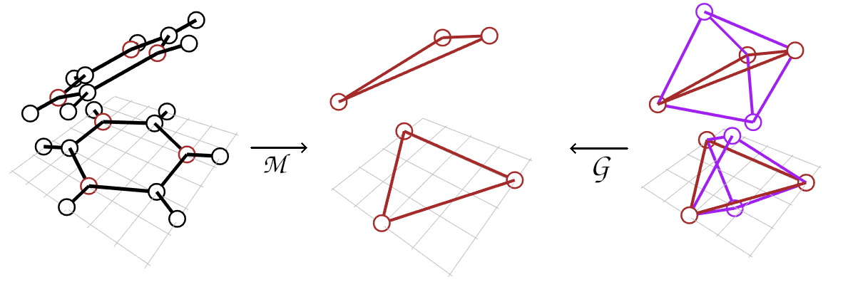
Figure 1: An example of virtual particle usage. The atomistic representation of benzene (left) is mapped via $\mathpzc{M}$ to a CG representation (center) only preserving three carbons (red). The full CG representation (right) of the same configuration has these three carbons and two additional virtual sites (purple) to help a pairwise potential capture the correct PMF. These sites are removed upon application of the virtual particle map $\mathpzc{G}$. These virtual sites have no atomistic counterpart.

Description of the formalism encompassing these situations requires us to suitably expand our notation. We still consider all distributions described previously but use the following modifications: first, samples from ${p_{\text{mod}}}$ are no longer generated by a simulation using the approximated PMF as its Hamiltonian. Instead, these samples are produced via a new mapping operator $\mathpzc{G}$ and simulation of a new finer grained representation characterized by ${p^{\text{pre}}_{\text{mod}}}$ via its own Hamiltonian $\left(\sum_{i=1}^{\nu}\mathpzc{p}_{i}^{2}/2\mathpzc{m}_{i}+{U^{\text{pre}}_{\text{mod}}}(\mathpzc{r}^{3\nu})\right)$ where $\mathpzc{m}_{i}$ are the masses at the pre-CG resolution. As a result, ${p_{\text{mod}}}$ is redefined with the following relations.

$${p_{\text{mod},\mathbf{R}}}(\mathbf{R}^{3N}) := \int_{{\mathcal{X}{r}^{\text{pre}}}}{p^{\text{pre}}_{\text{mod},\mathpzc{r}}}(\mathpzc{r}^{3\nu})\delta({\mathpzc{G}{r}}(\mathpzc{r}^{3\nu})-\mathbf{R}^{3N})\mathrm{d}\mathpzc{r}^{3\nu}\;\;\;$$ (22)

$${p_{\text{mod},\mathbf{P}}}(\mathbf{P}^{3N}) := \int_{{\mathcal{X}{p}^{\text{pre}}}}{p^{\text{pre}}_{\text{mod},\mathpzc{p}}}(\mathpzc{p}^{3\nu})\delta({\mathpzc{G}{p}}(\mathpzc{p}^{3\nu})-\mathbf{P}^{3N})\mathrm{d}\mathpzc{p}^{3\nu}\;\;\;$$ (23)

The resulting relations between resolutions are summarized in fig. 2.

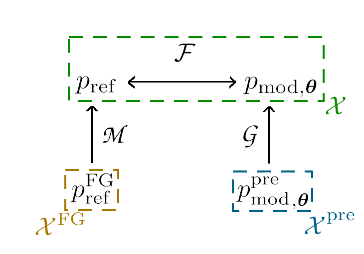
Figure 2: The relationship between resolutions when comparing FG and CG systems at a custom resolution, such as the case of virtual sites. Samples from the pre-CG domain ${\mathcal{X}^{\text{pre}}}$ (e.g., a CG configuration including virtual sites) are mapped to the CG domain $\mathcal{X}$ (e.g., a CG configuration without virtual sites) via $\mathpzc{G}$; samples from the FG domain ${\mathcal{X}^{\text{FG}}}$ (e.g., atomistic) are mapped to the same CG domain $\mathcal{X}$ via $\mathpzc{M}$. The mapped samples are then compared via $\mathcal{F}$.

Importantly, our training procedure needs two minor modifications. First, the variational estimation of divergences presented in Eq. (10) is composed solely of ensemble averages, which are approximated via sample averages; these averages can be evaluated by generating empirical samples from ${p_{\text{mod}}}$ via samples drawn from ${p^{\text{pre}}_{\text{mod}}}$ and application of $\mathpzc{G}$. This is a consequence of Eq. (24).

$$\langle f\rangle_{p_{\text{mod}}}=\langle f\circ\mathpzc{G}\rangle_{p^{\text{pre}}_{\text{mod}}}$$ (24)

Second, the gradients required for optimization of the parameters of the variational search (${\boldsymbol{\theta}}$) are calculable again through Eq. (24), allowing us to utilize our previous expression Eq. (15) at the resolution native to our new pre-CG Hamiltonian by minimizing the variationally optimized observable composed with $\mathpzc{G}$.

Importantly, while our examples in this section have primarily concerned situations in which fictional particles are added to the CG representation and then completely integrated over before calculating divergences, $\mathpzc{G}$ can easily be generalized. Fundamentally, it has the full flexibility of $\mathpzc{M}$; similarly, additional constraints are born from maintaining momentum consistency via methods described in the next subsection. However, if one discards momentum consistency, it is possible to maintain an intuitive pre-CG representation while nonlinearly modifying $\mathpzc{M}$ and $\mathpzc{G}$ to represent custom high-dimensional observables. In this case these mapped distributions are used for determining the quality of the pre-CG model. We reserve the bulk of our discussion and investigation of this more complex option to a future article.

II.5.1 Momentum Consistency

Previous sections have discussed the configurational variational statement central to ARCG; here, we discuss how to ensure momentum consistency. In the case that no pre-CG resolution is considered, momentum consistency in ARCG may be achieved through identical methods as stated in previous approaches, such as MS-CG.Noid et al. (2008a) However, when considering three distinct resolutions momentum consistency takes on a slightly modified form. We provide suitable constraints for a common case below, although extensions are straightforward.

Momentum consistency is characterized by the following equation:

$${p_{\text{ref},\mathbf{P}}}(\mathbf{P}^{3N})={p_{\text{mod},\mathbf{P}}}(\mathbf{P}^{3N}).$$ (25)

We here consider the specific case where both ${\mathpzc{M}_{\mathbf{r}}}$ and ${\mathpzc{G}{r}}$ are linear functions that satisfy the constraints defined in the MS-CG work:Noid et al. (2008a) ${\mathpzc{G}{r}}$ is limited to associate each CG site in ${\mathcal{X}^{\text{pre}}}$ unambiguously to at most a single site in $\mathcal{X}$ and has imposed translational and positivity constraints, and analogous constraints are placed on ${\mathpzc{M}_{\mathbf{r}}}$ (see appendix for more details). The momentum map ${\mathpzc{M}_{\mathbf{p}}}$ (and ${\mathpzc{G}{p}}$ with appropriate modifications) is assumed to take the following form as in reference 15:

$${\mathpzc{M}_{\mathbf{p}}}_{I}(\mathbf{p}^{3n}):=M{M}_{I}\sum_{i\in\mathcal{I}{M}_{I}}\frac{{c{M}_{Ii}}^{2}\mathbf{p}_{i}}{m_{i}},$$ (26)

In this case, previous work Noid et al. (2008a) has shown that the constants defining ${\mathpzc{M}_{\mathbf{p}}}$ (and similarly ${\mathpzc{G}{p}}$) can be combined with the masses of the sites contributing to a mapped site to provide a definition of the mapped masses (Eq. (27)) that define a Boltzmann distribution equal to the mapped momentum distribution

$$\left({M{M}_{I}}\right)^{-1}:=\sum_{i\in\mathcal{I}{M}_{I}}\frac{{c{M}_{Ii}}^{2}}{m_{i}},$$ (27)

where ${M{M}_{I}}$ is the mass of CG particle $I$ as implied by map $\mathpzc{M}$, $\mathcal{I}{M}_{I}$ is the set of all atoms that map to CG site $I$ according to map $\mathpzc{M}$, and $c{M}_{Ii}$ is the coefficient describing how the positions of FG particle $i$ contribute to CG particle $I$ according to map $\mathpzc{M}$. More generally, this implies that we can explicitly characterize the mapped momentum distributions for both the mapped FG and mapped CG systems, which when combined with Eq. (25) provides the following relation implying momentum consistency in a system with virtual particles

$$\exp\left(-\beta\sum_{I=1}^{N}\frac{\mathbf{P}_{I}^{2}}{2M{G}_{I}}\right) \propto \exp\left(-\beta\sum_{I=1}^{N}\frac{\mathbf{P}_{I}^{2}}{2M{M}_{I}}\right)$$ (28)

$$\left({M{G}_{I}}\right)^{-1} := \sum_{i\in\mathcal{I}{G}_{I}}\frac{{c{G}_{Ii}}^{2}}{\mathpzc{m}_{i}}.$$ (29)

The only solution to this equation is to set $M{G}_{I}=M{M}_{I}$ for each CG site $I$; in this case we find a set of equations implying consistency (Eq. (30)).

$$\left[0=\sum_{i\in\mathcal{I}{M}_{I}}\frac{{c{M}_{Ii}}^{2}}{m_{i}}-\sum_{i\in\mathcal{I}{G}_{I}}\frac{{c{G}_{Ii}}^{2}}{\mathpzc{m}_{i}}\right]\forall\text{ CG sites }I$$ (30)

Note that these equations are positively constrained with respect to masses and mapping constants (along with the previously stated constraints). This provides a simple condition connecting our FG masses, pre-CG masses, $\mathpzc{M}$, and $\mathpzc{G}$, and allows one to check for momentum consistency if all the relevant variables are defined. It is important to note that $I$ indexes the CG sites at the resolution of ${p_{\text{ref}}}$ and ${p_{\text{mod}}}$—that is, without the virtual particles. As such, in the case of $\mathpzc{G}$ simply dropping virtual particles consistency is trivially satisfied by simply matching the masses of the non dropped particles to those implied by the FG system with $\mathpzc{M}$. Additional details may be found in the appendix.

II.6 Related Methods

Despite differences in representation, ARCG can be formulated to elucidate connections to a variety of previous CG parameterization strategies, some of which have been mentioned in previous sections. This is performed via the appropriate design of the characteristic function space $\mathcal{Q}$ in Eq. (10). Additionally, ARCG bears resemblance to a recent CG method based on distinguishability and classification.Lemke and Peter (2017) In this section we make explicit connections between the $f$-divergence implementation presented in this article and such external methods. The applications of the $f$-divergence duality presented here are in the infinite sampling limit with a fully expressive variational search; in practice, significant differences in seemingly equivalent methods may arise.

Classification has been recently used to train a CG model by using the resulting decision function $\hat{\eta}^{\dagger}$ to directly update the CG configurational free energy.Lemke and Peter (2017) This is motivated by noticing that the $\eta$ that satisfies the variational bound in Eq. (17) can be related to the pointwise free energy difference as

$$\log\frac{1-\eta}{\eta}=\log{p_{\text{ref}}}-\log{p_{\text{mod}}},$$ (31)

suggesting a procedure where $\log(1-\hat{\eta})-\log(\hat{\eta})$ is scaled and used as an additive update to the CG potential. This procedure is similarly valid using any of the $f$-divergence losses discussed in this article.Reid and Williamson (2011) However, beyond the differing update rules, the variational divergence approach presented in this article is differentiated by a subtle but important difference in characteristic assumptions. The divergence interpretations of ARCG rely on the completeness of $\mathcal{Q}$, but place no constraint on $\{{p_{\text{mod},{\boldsymbol{\theta}}}}\}_{{\boldsymbol{\theta}}\in\mathbf{\Theta}}$, where $\mathbf{\Theta}$ denotes the set of all model parameterizations considered. In contrast, the interpretation of the method of Lemke and Peter (2017) also requires an fully expressive $\mathcal{Q}$; however, as the update to ${p_{\text{mod}}}$ inherently utilizes members of $\mathcal{Q}$, the method naturally also forces $\{{p_{\text{mod},{\boldsymbol{\theta}}}}\}_{{\boldsymbol{\theta}}\in\mathbf{\Theta}}$ to be fully expressive, i.e. ${p_{\text{ref}}}\in\{{p_{\text{mod},{\boldsymbol{\theta}}}}\}_{{\boldsymbol{\theta}}\in\mathbf{\Theta}}$. In other words, $\mathcal{Q}$ and $\{{p_{\text{mod},{\boldsymbol{\theta}}}}\}_{{\boldsymbol{\theta}}\in\mathbf{\Theta}}$ are directly coupled. As a result, in the case that the classifier used in the additive update method similarly has a relation to a specific $f$-divergence, an ideal model would always be chosen, rendering the specific choice of $f$-divergence inconsequential. Beyond this it is unclear how to expand the update rule of Lemke and Peter (2017) to apply to virtual sites, as the classifier is only directly present at the resolution of ${p_{\text{mod}}}$ and extension of the update to the resolution of ${p^{\text{pre}}_{\text{mod}}}$ is unclear.

REM CG proposes that approximate CG models should be parameterized by minimizing the relative entropy,Shell (2008) or KL-divergence, between the distributions produced at the FG resolution:

$$\int_{\mathcal{X}^{\text{FG}}}{p^{\text{FG}}_{\text{ref}}}(x)\log\left(\frac{{p^{\text{FG}}_{\text{ref}}}(x)}{p^{\text{FG}}_{\text{mod}}(x)}\right)\mathrm{d}x$$ (32)

where we have introduced a new quantity, $p^{\text{FG}}_{\text{mod}}$, defined to be the probability density implied by the CG model over FG space (which is not used in ARCG theory); the exact form implied over the FG space depends on the interpretation of REM CG considered.Rudzinski and Noid (2011) This differs by a constant (when considering CG force-field optimization) from the relative entropy considered at resolution of the CG model, given by

$$\int_{\mathcal{X}}{p_{\text{ref}}}(x)\log\left(\frac{{p_{\text{ref}}}(x)}{{p_{\text{mod}}}(x)}\right)\mathrm{d}x.$$ (33)

KL-divergence is an $f$-divergence (generated by $f(x):=x\log x$) and in the case of Eq. (33) can resultingly be formulated and solved for in the current framework, providing the following losses through Eq. (17)

$$l^{\text{RE}}_{\text{ref}}(h) = 2\left[\log\left(\frac{1-h}{h}\right)-1\right]$$ (34)

$$l^{\text{RE}}_{\text{mod}}(h) = 2\frac{h}{1-h}.$$ (35)

We utilize this method for the computational examples presented in Sec. III. We note that the full specification of REM CG considers comparing a coarser CG model to a finer FG model at the FG resolution by defining a new model density at the FG resolution ($p^{\text{FG}}_{\text{mod}}$), as where we have used many-to-one functions to reduce the resolution of the FG and pre-CG model in our theoretical approach. However, calculation of the relative entropy at CG resolution produces the same model selection rule as the FG relative entropy when considering the CG force-field. Optimization of systems with virtual particles is not straightforward via REM CG as most refinement schemes require $\langle\partial_{\boldsymbol{\theta}}{U_{\text{mod}}}_{\boldsymbol{\theta}}\rangle$ which is difficult to calculate as the explicit form of ${U_{\text{mod}}}_{\boldsymbol{\theta}}$ is unknown in the case of virtual particles.

Schöberl, Zabaras, and Koutsourelakis (2017) extended REM CG by framing coarse-graining as a generative process where the FG statistics are non-deterministically produced by the CG variables by means of a backmapping operator, a method termed Predictive Coarse-Graining (PCG). This approach allows optimization of the backmapping operator itself and additionally allows more flexibility in describing the connection between the FG and CG systems. This allows PCG to describe CG models with virtual particles. Additionally, PCG is trained using expectation-maximization, which can be framed as a two part process with a variational search providing the information for a gradient update of the parameters. PCG differs from ARCG in multiple ways. First, PCG aims to optimize an iteratively tightened lower bound on the relative entropy of the CG model, whereas ARCG encompasses the optimization of a larger variety of possible metrics, including relative entropy. Additionally, the variational estimation in PCG is solved via a closed form expression and generates a gradient update which optimizes said lower bound, as where the variational optimization in ARCG is solved iteratively in practice and provides the exact gradient of relative entropy. Finally, ARCG is not formulated as generating statistics at the FG resolution and instead is formulated on the CG resolution. Despite these differences, the overall similarity between PCG and ARCG suggests that the two methods could be used to extend each other. We reserve a detailed analysis of these connections for a future work.

Alternatively, recent work by Vlcek and Chialvo (2015) (as well as previous work by Stillinger (1970)) suggests that the Bhattacharyya distance ($BD$) Eq. (37) is a natural metric to judge approximate models.

$$BC({p_{\text{mod}}},{p_{\text{ref}}}) := \int_{\mathcal{X}}\sqrt{{p_{\text{mod}}}(x){p_{\text{ref}}}(x)}\mathrm{d}x$$ (36)

$$BD({p_{\text{mod}}},{p_{\text{ref}}}) := -\log BC({p_{\text{mod}}},{p_{\text{ref}}})$$ (37)

While the Bhattacharyya distance is not an $f$-divergence, it is related to one via a monotonic transformation: the Hellinger distance ($H$)

$$H({p_{\text{mod}}},{p_{\text{ref}}}) := \sqrt{1-BC({p_{\text{mod}}},{p_{\text{ref}}})}$$ (38)

$$= \mathbb{I}_{\left(\sqrt{t}-1\right)^{2}}({p_{\text{mod}}},{p_{\text{ref}}}).$$ (39)

This can be variationally approximated in the same framework as REM CG, resulting in the following losses:

$$l^{H}_{\text{mod}}(h) = 2\sqrt{\frac{h}{1-h}}$$ (40)

$$l^{H}_{\text{ref}}(h) = 2\sqrt{\frac{1-h}{h}}.$$ (41)

Justification of the Bhattacharyya distance may be grounded in information geometry and the distinguishability of samples produced by the FG and CG models. Despite the apparent similarity to the fictional game described earlier, the justification of Vlcek and Chialvo (2015) is grounded in distinguishing populations via their collective empirical samples, while our game focuses on distinguishing individual configurations. The stated connection simply occurs through our duality with $f$-divergences.

Inverse Monte Carlo (IMC),Lyubartsev and Laaksonen (1995) also known as Newton Inversion (NI), minimizes an observable that characterizes the difference between the mapped FG and CG systems (often through their radial distribution functions) and may be used on systems with virtual particles. The distributions utilized for this comparison are often low dimensional and are calculated via traditional binning approaches. ARCG may be viewed similarly as minimizing the expected value of observables; however in ARCG the observable minimized at each step of optimization must be variationally found, and subsequently changes from step to step. However, due to the envelope theorem, the derivatives calculated for both ARCG and IMC/NI share a similar covariance form shown in Eq. (15). Additionally, the typical approach in IMC/NI requires histograms to calculate the desired empirical correlation functions, limiting the metric to low dimensional distributions; ARCG does not perform binning of any kind.

There exist additional CG methods that are difficult to directly compare to ARCG (e.g., references 13; 18; 11; 15; 14; 16). However, in general, most methods considered make assumptions that strongly inhibit virtual site application. Specifically, methods often assume that the CG potential (or its derivatives) can be applied at the resolution of the CG samples acquired (either through calculation of the residual or the update strategy facilitating optimization), although extensions are sometimes feasible. For example, traditional MS-CG force-matching optimizes the CG force-field to optimally match mapped forces; with a general linear $\mathpzc{G}$ and ${U^{\text{pre}}_{\text{mod}}}$ this would likely require an iterative procedure to determine the mean force implied at the CG resolution by $\mathpzc{G}$ and ${U^{\text{pre}}_{\text{mod}}}$. Alternatively, gYBG inverts two- and three-body CG correlations to produce a force-field at the corresponding resolution of the observed correlations; similarly, Iterative Boltzmann Inversion requires a map to define the iterations that connect modifications in the potential to changes in the observed correlations (which is nonintuitive when considering parameters associated with general virtual sites). These limitations often do not appear to be fundamental ones, but rather one of implementation; extensions to these methods that circumvent this limitation are likely possible. There are three straightforward strategies to remove this limitation, the first two of which the authors know are in current use. First, several methods such as binning or kernel density estimation are used to approximate the probability density at a resolution differing from the CG configurational Hamiltonian (e.g., the radial distribution approach in reference 24). This approach is often limited to lower dimensional spaces when comparing models. Second, constraints are placed on virtual sites such that ${U^{\text{pre}}_{\text{mod}}}$ may be related via closed expression to ${U_{\text{mod}}}$.Jin, Han, and Voth (2019) This approach inherently requires limiting the type of virtual site considered. Third, methods that allow the observed mapped FG sample to be backmapped to the pre-CG domain are applied and then traditional approaches are used on the backmapped sample. In contrast, ARCG is well suited to higher dimensions, imposes no constraint on the virtual sites, and does not require backmapping; however, it incurs increased training complexity.

Finally, we note that while there is significant overlap between ARCG and GANs with respect to the residual calculation and optimization, the method by which samples are produced in the models is conceptually distinct. GANs are characterized by transforming noise to a fit a desired distribution; the optimization of the model parameters modifies the nature of this transformation. In contrast, the transformation present in ARCG is held constant, while the underlying sample generating process is modified.

III Implementation

Previous sections have provided abstract descriptions of the ARCG method, including the specific form with connection to $f$-divergences. In this section we provide the corresponding concrete expressions for optimizing models using relative entropy by implementing the classification based approach described in Sec. II.4. Additional practical points on implementation, relaxations of the method for stability, and the specification of $\mathcal{Q}$ are also discussed.

As previously noted, the relative entropy between ${p_{\text{ref}}}$ and ${p_{\text{mod}}}$ is an $f$-divergence and is obtained by setting $f(x):=x\log x$. This implies equivalence with a classification task with the aforementioned losses in Eq. (34), from which we derive the model optimization statement using Eq. (18) and associated gradients using Eq. (15), such that

$$\mathcal{F}^{\text{RE}}\left[{p^{\text{pre}}_{\text{mod}}}_{\boldsymbol{\theta}},{p_{\text{ref}}};\mathpzc{G}\right]=\max_{\hat{\eta}}\left\{-\left\langle\log\left(\frac{1-\hat{\eta}}{\hat{\eta}}\right)\right\rangle_{p_{\text{ref}}}-\left\langle\frac{\hat{\eta}\circ\mathpzc{G}}{1-\hat{\eta}\circ\mathpzc{G}}\right\rangle_{{p^{\text{pre}}_{\text{mod},{\boldsymbol{\theta}}}}}\right\}$$ (42)

$$\frac{\mathrm{d}}{\mathrm{d}{\boldsymbol{\theta}}_{i}}\mathcal{F}^{\text{RE}}\left[{p^{\text{pre}}_{\text{mod},{\boldsymbol{\theta}}}},{p_{\text{ref}}};\mathpzc{G}\right]=-\beta\left\langle\frac{\hat{\eta}^{\dagger}\circ\mathpzc{G}}{1-\hat{\eta}^{\dagger}\circ\mathpzc{G}}\right\rangle_{{p^{\text{pre}}_{\text{mod},{\boldsymbol{\theta}}}}}\left\langle\frac{\partial{U^{\text{pre}}_{\text{mod}}}_{\boldsymbol{\theta}}}{\partial{\boldsymbol{\theta}}_{i}}\right\rangle_{{p^{\text{pre}}_{\text{mod},{\boldsymbol{\theta}}}}}+\beta\left\langle\left(\frac{\hat{\eta}^{\dagger}\circ\mathpzc{G}}{1-\hat{\eta}^{\dagger}\circ\mathpzc{G}}\right)\frac{\partial{U^{\text{pre}}_{\text{mod},{\boldsymbol{\theta}}}}}{\partial{\boldsymbol{\theta}}_{i}}\right\rangle_{{p^{\text{pre}}_{\text{mod},{\boldsymbol{\theta}}}}}$$ (43)

. This comprises a full residual and associated gradient for optimization. However, in practice, the loss functions are poorly behaved: pointwise values of $\hat{\eta}=1$ easily create a divergent residual value (identical to the corresponding situation with the traditional relative entropy estimation methods). Fortunately, the optimal $\eta$ is shared among all proper losses.Reid and Williamson (2011) As a result, $\hat{\eta}^{\dagger}$ can be similarly discovered with the corresponding statement using the log-lossJames et al. (2013); Reid and Williamson (2011)

$$\hat{\eta}^{\dagger}=\operatorname*{arg\!\min}_{\hat{\eta}}\left\{\left\langle\log\hat{\eta}\right\rangle_{p_{\text{ref}}}+\left\langle\log(1-\hat{\eta}\circ\mathpzc{G})\right\rangle_{{p^{\text{pre}}_{\text{mod},{\boldsymbol{\theta}}}}}\right\}$$ (44)

while the gradient estimation remains unchanged. To summarize, the models trained in this article indirectly minimize Eq. (42) by producing derivatives over ${\boldsymbol{\theta}}$ via Eq. (44) and Eq. (43), where $\hat{\eta}^{\dagger}$ retains the same meaning across equations. This equality only holds assuming that $\hat{\eta}^{\dagger}=\eta$; incomplete $\mathcal{Q}$ can cause the resulting $\hat{\eta}^{\dagger}$’s to differ.

The numerical examples section IV are computed in the following way. First, the CG (or pre-CG) model is represented using a molecular force-field and samples are generated using standard molecular dynamics software. These samples are mapped if necessary using $\mathpzc{G}$. Reference examples are similarly generated and mapped using $\mathpzc{M}$ if needed. The variational estimator is represented using either a neural network or through logistic regression, which implement Eq. (44). The estimator then is trained on the reference and model samples. Finally, the gradient is calculated using the output of the variational estimator, Eq. (43), and the model samples; this gradient is then used to update the model parameters. This process is iterated, although the reference sample is not regenerated. The variational estimators are not fed the Cartesian coordinates of the input system directly; instead, various features are calculated for each frame, and these features are given as input to the variational estimator. This has the effect of constraining that $\hat{\eta}$ be a function of these features. Additional points on each of these details is discussed for each example or may be found in the appendix.

In some cases of ARCG, including the case of $f$-divergence estimation, the functions achieving the inner maximum with an complete $\mathcal{Q}$ can be expressed as a pointwise functions of the mapped distributions. Specifically, as noted in Eq. (19) the optimal witness function $\eta$ in the case of relative entropy is expressible as a function of the conditional class densities (${p_{\text{mod}}}$ and ${p_{\text{ref}}}$). This can guide how elements of a tractable $\mathcal{Q}$ are parameterized. When the algebraic forms of ${p_{\text{ref}}}$ and ${p_{\text{mod}}}$ are known to be functions of summary statistics of their respective systems (e.g., the inverse 6 and 12 moments in a traditional Lennard-Jones potentialLennard-Jones (1931)), we can often express an complete $\mathcal{Q}$ exactly with a manageable number of terms; however, this is not true of practical bottom-up CG application: the form of the mapping operator does not provide us with an algebraic understanding the implied mapped free energy surfaces. However, the resulting $\eta$ does share invariances with the free energy surfaces it is composed of (e.g., rotational and translational invariances).

The integrals characterizing the variational residual are computationally approximated as sample averages. Optimizing a function using a sample average introduces the possibility that the function which maximizes the sample average is a poor approximation of the function which maximizes population average. In the context of classification this error is captured by considering whether the classifier is overfitting the data sample. There are multiple strategies to overcome this;James et al. (2013) in the current study we use $l2$ regularization and only allow the variational estimator to update a limited number of times at each iteration. When optimizing examples with flexible potentials and large feature sets (for example, the water and methanol models presented in the next section), we have found that using a neural network quickly overfits the data provided, even with relatively strong regularization. However, reducing the number of iterations allowed at each step of variational optimization causes the neural network to exhibit considerable hysteresis between iterations, causing the force-field being optimized to orbit around an ideal solution. To ameliorate this we use logistic regression in these more complex cases, where the solution to the logistic regression is optimized using a limited number of iterations of l-BFGS. Note that the output of logistic regression readily affords estimates of the class conditional probabilities, which in turn directly connects its optimal solution to $\eta$.

The issues associated with overfitting and hysteresis are intrinsically connected the size of the finite samples used to approximate the integrals in Eq. (10). Overfitting would be reduced by increasing the sample size, which in turn would allow additional optimization at each variational iteration and would therefore reduce hysteresis. In practice, we have found that increasing the sample size to the point that the hysteresis is removed slows down the rate of force-field optimization considerably due to the time needed to both generate molecular samples and evaluate high dimensional gradients. This difficulty naturally suggests the use of modified sampling strategies to reduce the discrepancy between the sample and population averages. As Eq. (10) only involves expectation values any modified sampling scheme which allows for the calculation of an unbiased ensemble average is a candidate for this strategy. It is worth noting that ARCG selects an optimal observable function based on the ensemble averages of a large set of candidate observables, and that the error for each observable may be different, complicating the use of variance reduction techniques which are designed for a single observable. It would also be possible to improve the sampling of the feature space on top of which $\mathcal{Q}$ is represented; for example, if $\mathcal{Q}$ is represented by a neural network acting on two statistics calculated for each sample, free energy estimation may be used to better resolve the joint distribution of these two statistics themselves. This approach could be extended to produce an parameterization method which improves the observable estimates on the fly, such as that in Abrams and Vanden-Eijnden (2012). While we have not pursued these strategies here, future applications to more complex systems will likely need consider these options.

The variational search over possible $\hat{\eta}$ was either performed via a neural network outputting class probability predictions penalized via the log-loss or through logistic regression. Logistic regression was used in the cases of examples using $b$-spline based potentials and neural networks were used in all other cases. All neural networks used in examples in this paper utilized a simple feed-forward architecture with at least two layers (not including the input and output layer). The results were found to be insentive to the architecture chosen, and the specific architectures used may be found in appendix D. All internal nodes used rectified linear activation functions with the output normalized via softmax. The duality with classification underpins the utility such traditional choices have in our variational search.

In practice, we have noticed that ARCG optimization may suffer from instability, especially when optimizing the parameters of a model that produces a distribution significantly different than its optimization target. This issue can be noted by observing that the classifier achieves 100% accuracy during parameterization, producing uninformative gradients. In these cases we find that an effective strategy is to introduce standard Gaussian noise into both the model and reference samples; the variance of this noise is gradually reduced to zero as the optimization progresses. It is likely that a correct local minima is achieved in this case as the optimization appears stationary at the end of minimzation, but it is unclear if the selection of a specific local minima is biased using this strategy.

A public proof-of-concept python/Lammps based implementation is available at the weblink https://github.com/uchicago-voth/ARCG. This code base makes extensive use of the theano, theanets, pyLammps, numpy, scikit, and dill libraries. All computational examples presented in this paper may be found in the test portion of this code, which includes the complete settings used to generate the data used. Visualizations and analysis were performed with the matplotlib and seaborn libraries, as well as the base plotting system, rgl, and data.table packages in R. Extensions providing scalability for more complex systems and potentials will be considered in future work.

IV Results

The relative entropy approach described in section III was applied to five test systems. First, a simple single component 12-6 Lennard-Jones (LJ) system was optimized to approximate a reference LJ system at the same resolution (no virtual particles were present, and no coarse-graining of either the reference or model was performed). Second, a system representing two bonded real particles where force is partially mediated by a single harmonically bonded virtual particle was optimized to approximate a reference system of the same type. Third, a binary LJ liquid undergoing phase separation was simulated and optimized after particles of a single type had been integrated out; this distribution was fit to match a similarly integrated binary LJ system. Fourth, a CG model using pairwise $b$-spline interactions and a single site per molecule was used to approximate liquid methanol. Fifth, a CG model using pairwise $b$-spline interactions and a single site per molecule was used to approximate liquid water. In these cases we observed good convergence of suitable correlation functions; however, in cases with virtual particles we found that numerically recovering the known parameters of the reference system is difficult; in other words, it seems likely that the parameter space is either redundant or sloppy,Transtrum et al. (2015) with similar correlation functions arising from distinct parameter sets. We note that while the potentials considered here are relatively simple, ARCG is fully applicable to more complex potentials such as those in Zhang et al. (2013).

The first three examples considered here are theoretically able to capture the reference distributions used for fitting (i.e., the model optimized is not misspecified). This is ensured by generating reference data using a force-field that is directly representable by the CG force-field family. For example, the LJ CG model in the first example was optimized to reproduce the statistics generated by a particular LJ reference potential. Additionally, when either the reference or model are modified using a mapping function, this mapping operator is forced to be the same between the two systems, and the reference data is again produced using a force-field which is expressible by the CG model. For example, in the case of the virtual solvent LJ system, a distinct system of binary LJ particles was simulated for both the model and reference data samples, each with differing parameter sets. Both systems then had the particles of a specific shared type integrated out. The resulting integrated distributions were then the basis of comparison used to train the model parameters (with new statistics being created for the CG model at each iteration). This is not true for the examples approximating water and methanol: here, the CG model is approximating the mapped distributions using a pairwise potential and is unable to capture the true free energy surface.

IV.1 Lennard-Jones Fluid

A single component 12-6 LJ fluid was simulated with 864 particles at 300K (the potential form is given in Eq. (45) with $r_{ij}$ denoting the Euclidean distance between particles $i$ and $j$).

$$U(\mathbf{R}^{3N})=4\epsilon\sum_{i>j}\left[\left(\frac{\sigma}{r_{ij}}\right)^{12}-\left(\frac{\sigma}{r_{ij}}\right)^{6}\right]$$ (45)

The system was simulated at constant NVT conditions using a Langevin thermostat with coupling parameter set to 100.0 fs and a timestep of 1.0 fs. No virtual particles were present; i.e., $\mathpzc{G}$ and $\mathpzc{M}$ are set to be the identity function. Inverse sixth and twelfth moments were used as input to the variational estimator (in this case, this set of features is known to be complete, see appendix D for details). System $A_{\text{initial}}$ with $\epsilon_{A_{\text{initial}}}=0.6\text{kcal}/\text{mol}$ and $\sigma_{A_{\text{initial}}}=3.5{\mbox{\AA}}$ was optimized to match the statistics of system $B$ characterized by $\epsilon_{B}=0.75\text{kcal}/\text{mol}$ and $\sigma_{B}=3.0{\mbox{\AA}}$. Upon optimization, the parameters of $A$ were seen to quantitative converge to those of $B$: $\epsilon_{A_{\text{opt}}}=0.746\text{kcal}/\text{mol}$ and $\sigma_{A_{\text{opt}}}=3.00{\mbox{\AA}}$. Additionally, convergence of the pairwise correlation functions (fig. 3) was observed. The initial parameters of $A$ resulted in a homogeneous liquid, while those of system $B$ (and system $A$ upon optimization) resulted in liquid-vapor coexistence. During training Gaussian noise was used to smooth out initial gradients to resolve initial soft wall differences; this noise is reduced to zero by the end of optimization. Optimization was performed using RMSpropHinton, Srivastava, and Swersky (2012) with individual rates for each parameter. These results demonstrate good convergence properties with small parameter sets when no virtual particles are considered in the pre-CG resolution.

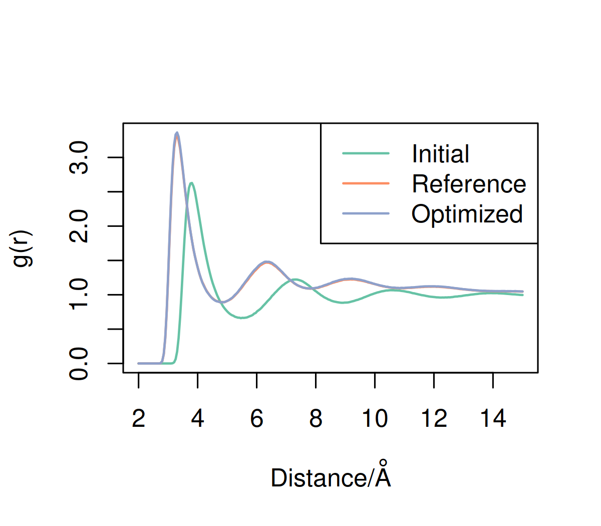
Figure 3: Radial distribution functions calculated for the unoptimized system $A_{\text{initial}}$, the reference system $B$, and the optimized system $A_{\text{opt}}$.

IV.2 Virtual Bond Site

A system of three particles completely connected via harmonic bonds was simulated at 300 K. The system was propagated in constant NVT conditions using a Langevin thermostat with coupling parameter set to 100.0 fs and a timestep of 1.0 fs. Two types of particles are present; we denote the types of the particles $X,Y,X$. Upon application of $\mathpzc{M}$ and $\mathpzc{G}$, the $Y$ particle is removed, resulting in a system composed of two particles of type $X$ (i.e., the $Y$ particle is a virtual site). This mapped system is optimized using the distance between the two $X$ particles as input to the discriminator; in this case, this feature set is complete. Initial, optimized, and reference parameters are seen in table 1.

System	$x_{XY}/{\mbox{\AA}}$	$k_{XY}/\frac{\text{kcal}}{\text{mol}}{\mbox{\AA}}^{-2}$	$x_{XX}/{\mbox{\AA}}$	$k_{XX}/\frac{\text{kcal}}{\text{mol}}{\mbox{\AA}}^{-2}$
$B$	2	2.7	2.3	0.4
$A_{\text{initial}}$	0.65	2.2	1.4	0.15
$A_{\text{opt}}$	1.70	2.06	2.66	0.224

Table 1: Parameters for systems with virtual bonded sites. $x$ denotes the zero energy point of the bond while $k$ denotes bond strength. Subscripts specify the particle types between which the bond acts. System $A_{\text{initial}}$ was optimized to match system $B$, resulting in $A_{\text{opt}}$.

Optimization was performed using RMSprop. Convergence to a specific parameter set that reproduces observed correlations (fig. 4) is fast; however these parameters differ from the parameters of the reference system. Additional simulations were run where the CG model was initialized with parameters set to those of the reference system (results not shown); in this case, we observed local diffusion around a small set of parameters including the true set. This suggests that virtual particles may create degeneracy in model specification in practice (i.e., even if the model parameters are identifiable, the specification is sloppy).

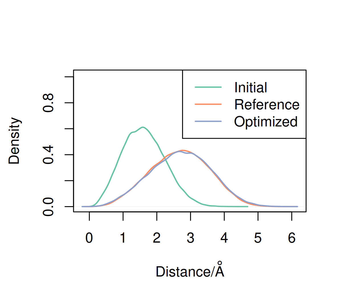
Figure 4: Bond distance distribution functions calculated for the unoptimized system $A_{\text{initial}}$, the reference system $B$, and the optimized system $A_{\text{opt}}$.

This case represents an application where a pairwise force-field may be augmented via bonded virtual particles to create modified correlations. For example, a heterogeneous elastic networkLyman, Pfaendtner, and Voth (2008) may be augmented by introducing virtual particles to facilitate higher order correlations.

IV.3 Virtual Solvent Lennard-Jones Fluid

A binary system composed of 864 LJ particles of types $X$ and $Y$ was simulated at 300 K. The system was simulated at constant NVT conditions using a Langevin thermostat with coupling parameter set to 100.0 fs and a timestep of 1.0 fs. Equal numbers of $X$ and $Y$ particles were present prior to the application of mapping operators; upon application all particles of type $Y$ were removed (i.e., the $Y$ particles are virtual sites). The target system was parameterized to undergo phase coexistence, while the unoptimized CG model was well mixed. Parameters are found in table 2. Optimization was performed using RMSprop with rates adjusted for each parameter. Gaussian noise was used to stabilize initial training. Visual inspection of representative molecular configurations showed greatly improved similarity for the optimized parameter set (fig. 5). Again, while convergence of correlation functions is readily observed (fig. 6), parameters do not converge to those of the reference system, likely due to sloppiness in specification.

System	$\sigma_{XX}/{\mbox{\AA}}$	$\epsilon_{XX}/\frac{\text{kcal}}{\text{mol}}$	$\sigma_{YY}/{\mbox{\AA}}$	$\epsilon_{YY}/\frac{\text{kcal}}{\text{mol}}$	$\sigma_{XY}/{\mbox{\AA}}$	$\epsilon_{XY}/\frac{\text{kcal}}{\text{mol}}$
$B$	0.7	3.6	0.7	3.6	0.35	3.5
$A_{\text{initial}}$	0.6	3.5	0.6	3.2	0.5	3.1
$A_{\text{opt}}$	0.713	3.600	0.722	3.594	0.349	3.494

Table 2: Parameters for systems with virtual bonded sites. $x$ denotes the zero energy point of the bond while $k$ denotes bond strength. Subscripts specify the particle types between which the bond acts. System $A_{\text{initial}}$ was optimized to match system $B$, resulting in $A_{\text{opt}}$.

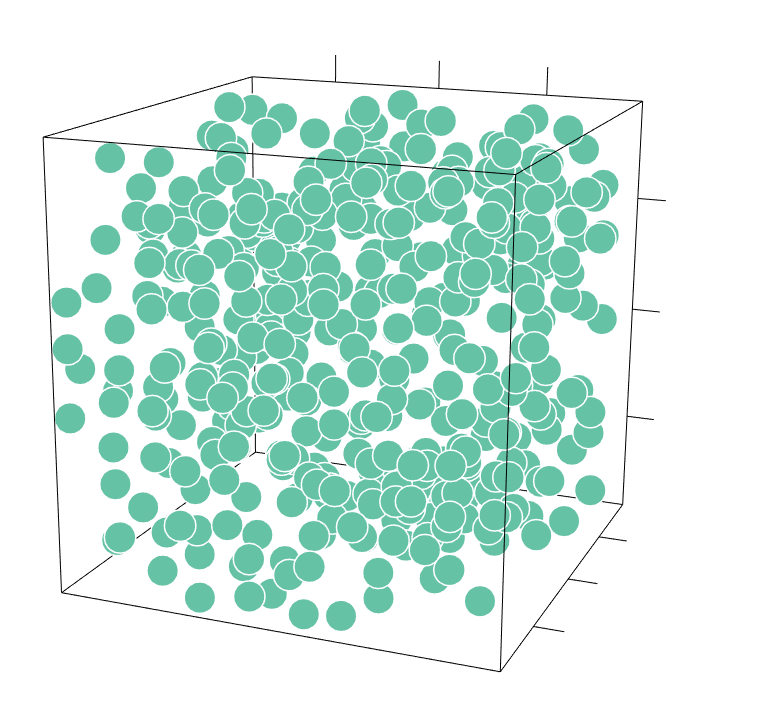
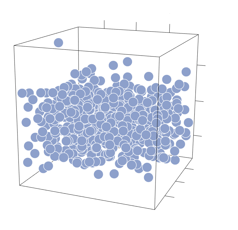
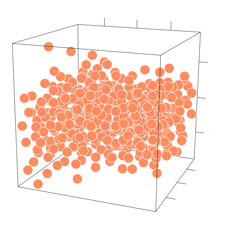
Figure 5: Sample configurations of the unoptimized model (green), the optimized model (blue) and the reference data (orange). Configurations are shown at the resolution of comparison, i.e., after the application of $\mathpzc{M}$ and $\mathpzc{G}$. Slab type formation, similar to that present in the optimized model, is seen after parameter optimization.

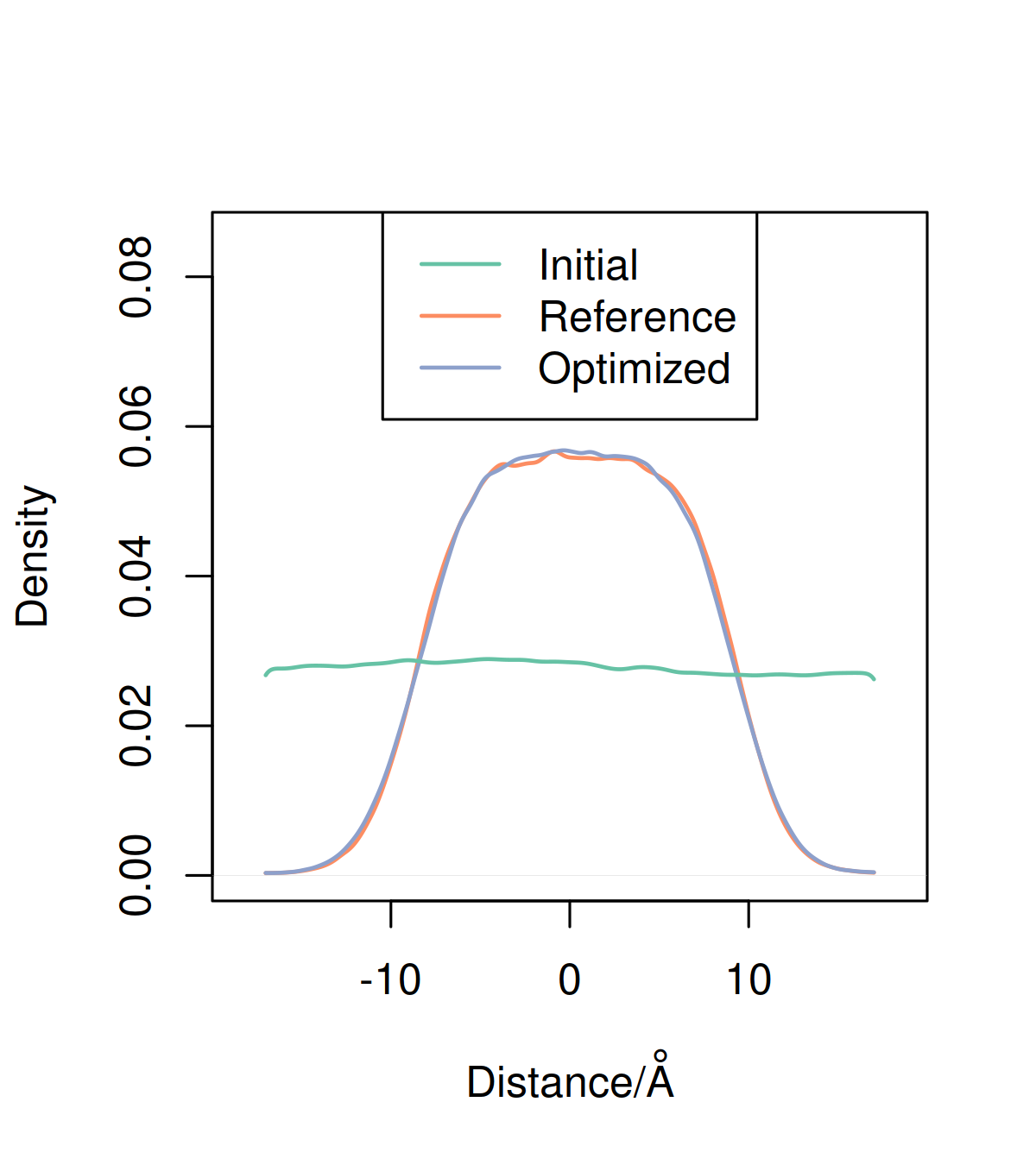
Figure 6: Probability densities across the slab type formations present in the integrated binary LJ systems (along the $z$ axis of the simulation box). No slab structure is present in the initial model.

This case is representative of the situation where higher order correlations may be captured by the addition of virtual solvent particles. For example, the hydrophobic driving force underlying a CG lipid bilayer could be facilitated by a virtual solvent. This is distinct from using traditional explicit solvent where each solvent molecule is directly connected to the FG reference system: there, the behavior of the solvent is incorporated into the quality of the model, as where the approach of ARCG ignores the direct solvent behavior.

IV.4 Single Site Methanol

Methanol was modeled using single site CG liquid. The reference atomistic (FG) trajectory of 512 molecules was simulated in the NVT ensemble at 300K with a Nose-Hoover damping time of 1 ps after NPT equilibration at 1 atm. The OPLS-AAJorgensen and Tirado-Rives (2005); Dodda et al. (2017a, b) forcefield was used in the atomistic system. The FG system was mapped to the to the CG resolution by retaining only the central carbon; no virtual sites were present in the CG system. The CG potential was described using a pairwise $b$-spline potential using 15 equally spaced knots and a 10 Å cutoff (the last three control points were set to zero to enforce a smooth decay at the cutoff). The CG system was run at the same temperature and volume as the FG system using a Langevin coupling parameter of 100 fs and a timestep of 1 fs. The starting potential used for the simulation was a WCA potential (fig 8). Quantitative reproduction of the radial distribution function was observed (fig 7). Convergence was smoothing using Gaussian noise whose standard deviation decayed to zero by the end of the optimization.

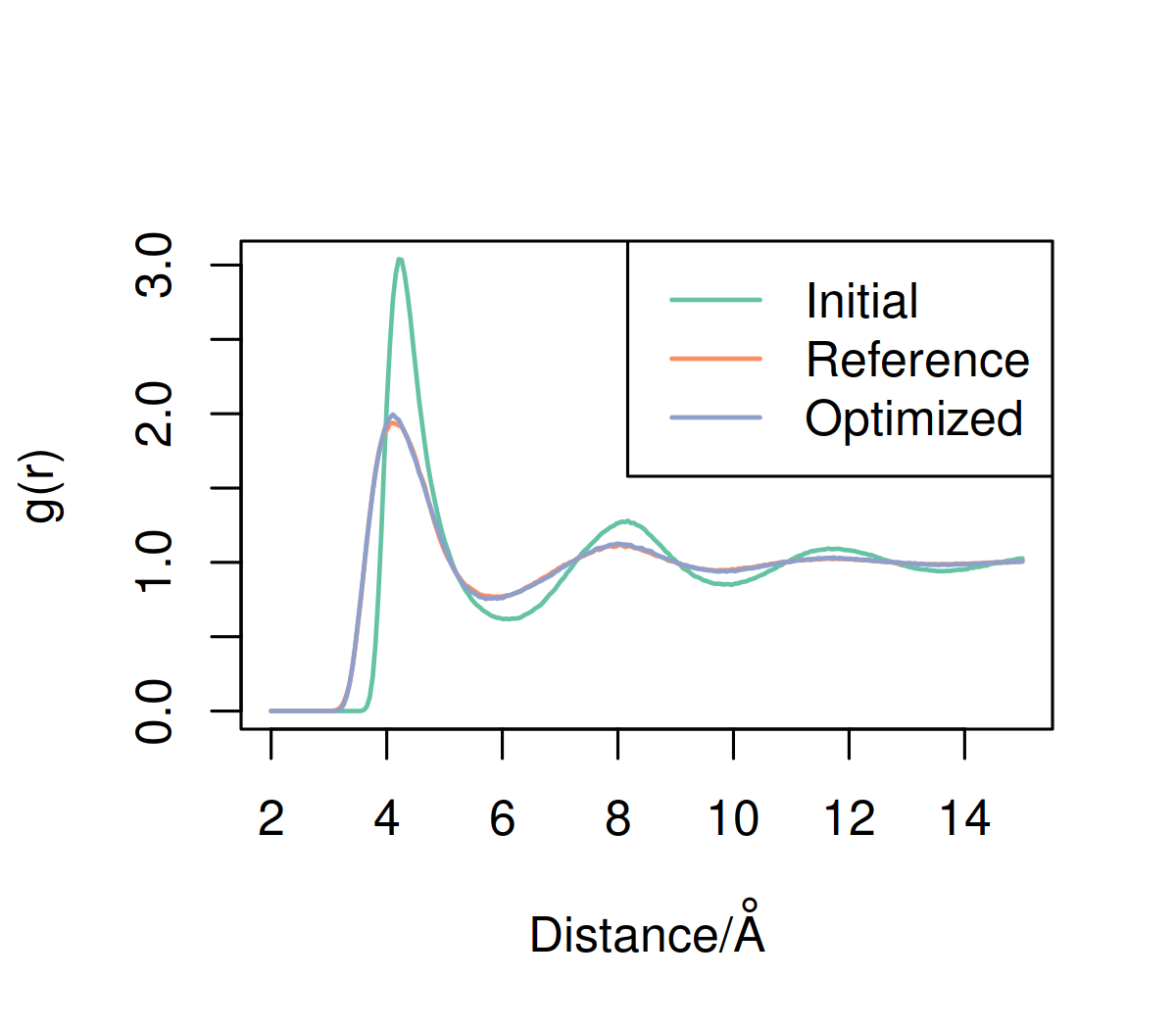
Figure 7: Radial distribution functions for the reference, initial, and optimized methanol systems. Note that the optimized and reference RDFs are nearly within line thickness.

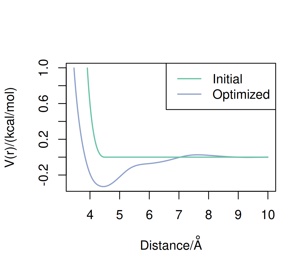
Figure 8: Pairwise potential functions characterizing the initial and optimized methanol systems.

IV.5 Single Site Water

A single site model of water was trained using 512 molecules of SPC/E water simulated at 300K. The molecular (FG) system was equilibrated at 1 atm and production NVT samples were produced with the Nose-Hoover thermostat with a 1 ps damping time. The mapping connecting the FG system to the CG system was the center of mass mapping; no virtual sites were present in the CG system. The CG system potential was limited to pairwise interactions with a 7 Å cutoff and was parameterized using $b$-splines with 37 knots (see appendix D for knot locations and further details). The last three spline control points were set to zero to enforce continuity at the cutoff. The starting potential used for the simulation was a WCA potential (fig 9). CG simulations were run at the same volume as the FG system with a Langevin thermostat, whose coupling parameter was set to 100 fs, and a 1 fs timestep. Quantitative reproduction of the radial distribution function was obtained (fig 10). Gaussian noise was used initially to smooth convergence and was tapered to a standard deviation of zero by the end of the optimization.

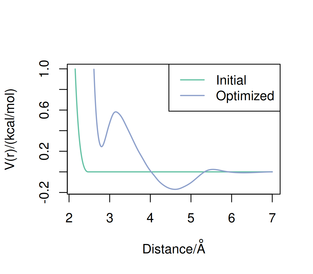
Figure 9: Pairwise potential functions characterizing the initial and optimized water systems.

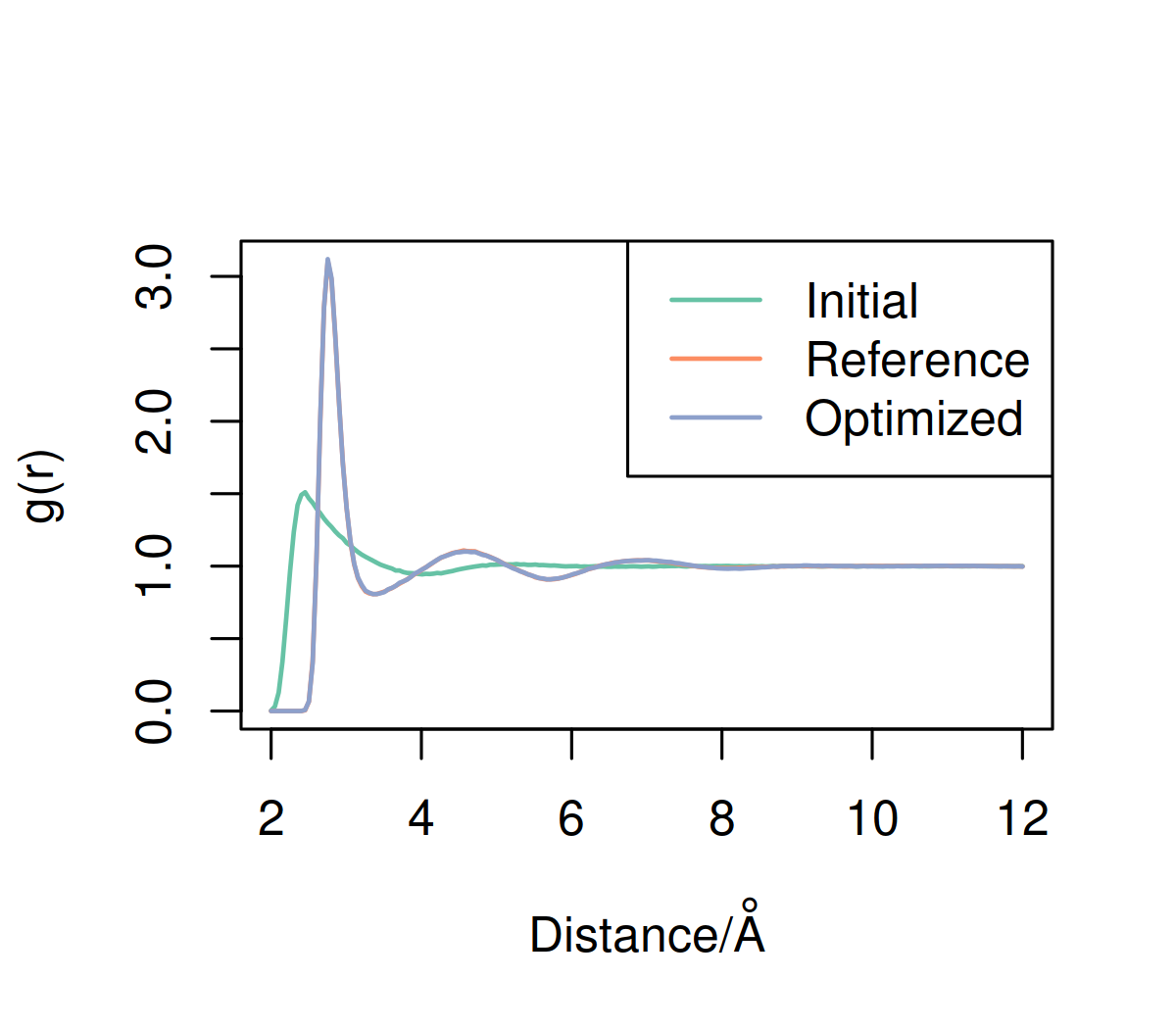
Figure 10: Radial distribution functions for the reference, initial, and optimized water systems. Note that the optimized and reference RDFs are within line thickness.

V Discussion

In previous sections we have described a broad new class of variational statements for optimizing CG models and described methods for their optimization by utilizing the theory underpinning adversarial models in ML. Subsequently we have shown that it is possible to parameterize a CG model via ARCG at a coarser resolution than that native to the CG Hamiltonian. A clear application of ARCG is the parameterization of models that contain virtual sites; however, the CG distribution may be critiqued at any coarser resolution, providing the intriguing ability to control what aspects of a CG model are visible for optimization purposes. In the process of doing so we showed that gradients needed at each step of divergence minimization can be reformulated as modifying the system Hamiltonian to minimize the value of a specific observable, but that this observable depends on the distributions being considered at that step of optimization. We note that more generally the method presented can be used to calculate the KL divergence (and any of the other divergences discussed) between distributions for which no probability density/mass is known and for which one cannot be approximated via kernel density approximation or binning.

Beyond our central results we have provided work and discussion on two supporting topics.

1. We have provided comparisons to multiple contemporary methods for CG parameterization. In certain cases we have shown that divergences characterizing their configurational variational principles can be used in ARCG modeling. In one case we showed that classifier based approaches bear striking but not complete similarity to the presented approach. In the remaining cases we have discussed how decoupling the resolution at which we critique a model from the resolution of the CG Hamiltonian creates difficulties in said approaches.

2. We have provided a set of sufficient conditions for momentum consistency in the case of virtual sites and described how these conditions may be extended. These are closely related to consistency requirements for traditional bottom-up CG models.

Additionally, we have provided simple numerical examples (and a public computational implementation) for which we have optimized CG potentials to match specific distributions, some of which utilize CG virtual particles. The results show quantitative agreement for calculated correlations, visual agreement, and qualitative agreement in matching exact coefficients when the answer is known (quantitative agreement is seen when virtual particles are not present). Difficulties in convergence appear to be either due to instability in the parameterization process or sloppiness in the model specifications. The manner in which this will affect realistic systems is yet to be seen, but may present a significant challenge. It is clear that in the most general case parameter uniqueness is not guaranteed: if CG consistency can be obtained without virtual particles, then a model that can both decouple the virtual particle interaction from the real particles and modify the behavior of the virtual particles independently of said coupling will inherently be nonidentifiable. Additionally, it is likely that in the case of $f$-divergence based ARCG optimization that a relatively good initial hypothesis for the CG potential may be necessary, or significant amounts of noise must be added initially during optimization.

There are multiple additional studies that could naturally expand and clarify the results presented.

1. The methods provided can be applied to approximate nontrivial molecular systems without virtual particles. This will require multiple steps: first, the proof-of-concept software framework presented will have to be expanded for larger system sizes. Second, the training method used will have to be developed such that it remains stable, whether through the systematic addition of noise or the use of enhanced sampling techniques. Third, the feature-space used to index $\mathcal{Q}$ will likely have to be correctly engineered based on knowledge of the FG and CG Hamiltonians. All three of these are tractable challenges.

2. The effect of using virtual particles should be investigated both computationally and theoretically, as previous analysis on incomplete basis sets (e.g., that on relative entropy and MS-CG Rudzinski and Noid (2011)) does not apply transparently. In the process of doing so a better theoretical understanding of how to utilize these methods to capture specific higher order correlations in the training data should additionally be investigated, possibly leading to new ways in which bottom-up CG parameterization may be tuned to reproduce specific novel correlation functions.

3. The effect of various divergences on training approximate CG models should be investigated theoretically and through simulation. This will facilitate the design of CG parameterization methods that have different biases in the approximations they produce when coupled with realistic CG potentials. This applies to not only to various $f$-divergences but also the wider set of divergences not heavily discussed in this article, such as the Wasserstein,Arjovsky, Chintala, and Bottou (2017) Sobolev,Mroueh et al. (2017) Energy,Bouchacourt, Pawan Kumar, and Nowozin (2016) and MMDDziugaite, Roy, and Ghahramani (2015) distances. The Wasserstein and Energy distances share the interesting property of taking into account the spatial organization of the domain of the probability distributions considered through a separate spatial metric. Combined with kinetically informed coordinate transforms such as TICAPérez-Hernández et al. (2013) and variants,Noé and Clementi (2015); Noé, Banisch, and Clementi (2016) it may be possible to parameterize models to have stationary distributions that are kinetically close to one another.

4. The effect of an incomplete $\mathcal{Q}$ should be investigated. In this case the presented divergence based interpretation is not trivially accurate.Liu and Chaudhuri (2018) Understanding of how imperfect classifiers affect the parameterization of approximate models may have large implications on the optimization of complex multicomponent systems; overly expressive $\mathcal{Q}$ will likely impede model parameterization as more sampling of the CG and FG system may be required.

VI Concluding Remarks

In this article we discussed a new class of methods for the systematic bottom-up parameterization of a CG model. In doing so we illustrated concrete connections between CG models and algorithms such as generative adversarial networks. Utilizing these connections we both decoupled the resolution at which we critique our CG model from the CG potential itself and enabled the use of a variety of novel measures of quality for CG model parameterization. We provided a proof of concept implementation and several numerical examples. Additionally, we illustrated precise connections to several previous methods for CG model parameterization. Finally, we noted multiple future branches of studies that can now be pursued. Together, these results open a new conceptual basis for future systematic CG parameterization strategies.

Appendix A Envelope Theorem

The envelope theorem is used to justify optimizing ${\boldsymbol{\theta}}$ using only the partials calculated holding the optimal observable constant. A general statement of the envelope theorem is given by theorem 1 in Milgrom and Segal (2002), which also notes that the theorem applies to directional derivatives in a normed vector space.

Let $X$ denote the choice set and let the relevant parameter be $t\in[0,1]$. Let $f:X\times[0,1]\to\mathbf{R}$ denote the parameterized objective function. The value function $V$ and the optimal choice correspondence $X^{*}$ are given by:

$$V(t):=\sup_{x\in X}f(x,t)$$ (46)

$$X^{*}(t):=\{x\in X:f(x,t)=V(t)\}$$ (47)

Take $t\in(0,1)$ and $x^{*}\in X^{*}(t)$, and suppose that $\partial_{t}f(x^{*},t)$ exists. If $V$ is differentiable at $t$, then $V^{\prime}(t)=\partial_{t}f(x^{*},t)$.

This result puts no constraint on $X$, which corresponds to $\mathcal{Q}$ in the current work, except that its maximal member have a derivative at that point. Additionally, as noted in Milgrom and Segal (2002), this results is only useful if $V$ is known to be differentiable. This is compatible with our $f$-divergence variational statement when considered in the context of a complete $\mathcal{Q}$ and population averages, but must in general be confirmed for each choice of $\mathcal{Q}$. In situations where a closed form expression corresponding to the maximum is not known, constraints may be put on each member of $\mathcal{Q}$ to ensure applicability. Suitable constraints may be found in the remainder of Milgrom and Segal (2002).

Appendix B Momentum Consistency

The described approach to achieve momentum consistency requires that we put more specific constraints on $\mathpzc{G}$. This is needed due to our minimal strategy for providing sufficiency conditions for consistency: primarily, we utilize arguments in previous work to provide sufficient constraints. The resulting conditions given suffice for the case of virtual particles that are simply dropped from the system by $\mathpzc{G}$. Generalizations to linear mappings that share particles between sites can additionally be inferred. First we discuss the approach of previous work on momentum consistency as is relevant to our work, and then concisely give a route to momentum consistency.

B.1 MS-CG

Generally, we will here assume that ${\mathpzc{M}_{\mathbf{r}}}$ satisfies specific properties. Once ${\mathpzc{M}_{\mathbf{r}}}$ is defined, we construct an appropriate ${\mathpzc{M}_{\mathbf{p}}}$. First, ${\mathpzc{M}_{\mathbf{r}}}$ must be expressible in the following linear form, where ${\mathpzc{M}_{\mathbf{r}}}_{I}$ denotes the $I$th particle entry of the output of ${\mathpzc{M}_{\mathbf{r}}}$, $i$ iterates over the particles contribute to site $I$, and $c$ denotes positive constants.

$${\mathpzc{M}_{\mathbf{r}}}_{I}(r^{n}):=\sum_{i=1}^{n{M}_{I}}c^{{\mathpzc{M}_{\mathbf{r}}}}_{Ii}r_{i}$$ (48)

As in MS-CG,Noid et al. (2008a) we impose translational consistency.

$$\sum_{i=1}^{n{M}_{I}}c^{{\mathpzc{M}_{\mathbf{r}}}}_{Ii}=1$$ (49)

From this we allow ${\mathpzc{M}_{\mathbf{r}}}$ to imply ${\mathpzc{M}_{\mathbf{p}}}$ up to the factor of the CG masses $\{M_{I}\}_{I}$ as stated in MS-CG.

$${\mathpzc{M}_{\mathbf{p}}}_{I}(\mathbf{\mathbf{p}}^{n}):=M_{I}\sum_{i=1}^{n{M}_{I}}\frac{c_{Ii}\mathbf{p}_{i}}{m_{i}}$$ (50)

As before, this type of map transforms global consistency into constituent momentum and position space components, i.e.,

$${p_{\text{mod}}}(\mathbf{R}^{3N},\mathbf{P}^{3N})=\int\mathrm{d}\mathbf{r}^{3n}\int\mathrm{d}\mathbf{p}^{3n}{p^{\text{pre}}_{\text{mod}}}(\mathbf{r}^{3n},\mathbf{p}^{3n})\delta({\mathpzc{M}_{\mathbf{r}}}(\mathbf{r}^{3n})-\mathbf{R}^{3N})\delta({\mathpzc{M}_{\mathbf{p}}}(\mathbf{p}^{3n})-\mathbf{P}^{3N})={p_{\text{mod},\mathbf{R}}}(\mathbf{R}^{3N}){p_{\text{mod},\mathbf{P}}}(\mathbf{P}^{3N})$$ (51)

where the vector valued delta functions are understood to be products of scalar delta functions. If $\mathpzc{M}$ does not associate any individual atoms to more than a single CG site, then

$$\exp\left(-\beta\sum_{I=1}^{N}\frac{\mathbf{P}_{I}^{2}}{2M_{I}}\right) \propto \int\mathrm{d}\mathbf{p}^{3n}\exp\left(-\beta\sum_{i=1}^{n}\frac{\mathbf{p}_{i}^{2}}{2m_{i}}\right)$$ (52)

$$\times\delta({\mathpzc{M}_{\mathbf{p}}}(\mathbf{p}^{3n})-\mathbf{P}^{3N})$$

with

$${M{M}_{I}}^{-1}:=\sum_{i\in\mathcal{I}_{I}}\frac{{c{M}_{Ii}}^{2}}{m_{i}}$$ (53)

We will additionally assume that analogous constraints are put on ${\mathpzc{G}{r}}$ when considering momentum consistency below.

B.2 Momentum Consistency

Using these points we now move forward directly discussing momentum consistency. As stated previously, by constraining $\mathpzc{G}$ and $\mathpzc{M}$ as above, and assuming the underlying systems are characterized by separable probability densities, we find

$${p_{\text{mod}}}(\mathbf{R}^{3N},\mathbf{P}^{3N}) = {p_{\text{mod},\mathbf{R}}}(\mathbf{R}^{3N}){p_{\text{mod},\mathbf{P}}}(\mathbf{P}^{3N})$$ (54)

$${p_{\text{ref}}}(\mathbf{R}^{3N},\mathbf{P}^{3N}) = {p_{\text{ref},\mathbf{R}}}(\mathbf{R}^{3N}){p_{\text{ref},\mathbf{P}}}(\mathbf{P}^{3N})$$ (55)

As a result, we split up our consistency statement (omitting arguments for clarity)

$$\left({p_{\text{mod},\mathbf{R}}}={p_{\text{ref},\mathbf{R}}}\land{p_{\text{mod},\mathbf{P}}}={p_{\text{ref},\mathbf{P}}}\right)\implies{p_{\text{mod}}}={p_{\text{ref}}}$$ (56)

Configurational consistency is handled via divergence matching as described in the main article; we here consider momentum consistency algebraically.

$${p_{\text{mod},\mathbf{P}}}={p_{\text{ref},\mathbf{P}}}\iff\int\mathrm{d}\mathpzc{p}^{3\nu}\exp\left(-\beta\sum_{i=1}^{\nu}\frac{\mathpzc{p}_{i}^{2}}{2\mathpzc{m}_{i}}\right)\delta({\mathpzc{G}{p}}(\mathpzc{p}^{3\nu})-\mathbf{P}^{3N})\propto\int\mathrm{d}\mathbf{p}^{3n}\exp\left(-\beta\sum_{i=1}^{n}\frac{\mathbf{p}_{i}^{2}}{2m_{i}}\right)\delta({\mathpzc{M}_{\mathbf{p}}}(\mathbf{p}^{3n})-\mathbf{P}^{3N}).$$ (57)

We substitute these using two sets of properly designed CG masses, each set implied by a mapping operator and the masses at resolution it maps

$$\exp\left(-\beta\sum_{I=1}^{N}\frac{\mathbf{P}_{I}^{2}}{2M{G}_{I}}\right) \propto \exp\left(-\beta\sum_{I=1}^{N}\frac{\mathbf{P}_{I}^{2}}{2M{M}_{I}}\right)$$ (58)

$${M{G}_{I}}^{-1} := \sum_{i\in\mathcal{I}{G}_{I}}\frac{{c{G}_{Ii}}^{2}}{\mathpzc{m}_{i}}$$ (59)

$${M{M}_{I}}^{-1} := \sum_{i\in\mathcal{I}{M}_{I}}\frac{{c{M}_{Ii}}^{2}}{m_{i}}$$ (60)

The only solution is to set $M{G}_{I}=M{M}_{I}$ for each CG site $I$; in this case find a set of equations implying consistency.

$$\left[0=\sum_{i\in\mathcal{I}{M}_{I}}\frac{{c{M}_{Ii}}^{2}}{m_{i}}-\sum_{i\in\mathcal{I}{G}_{I}}\frac{{c{G}_{Ii}}^{2}}{\mathpzc{m}_{i}}\right]\forall\text{ CG sites }I$$ (61)

Note that these equations are still subject to the aforementioned constraints (positivity, etc.). This provides a simple condition connecting our FG masses, pre-CG masses, $\mathpzc{M}$, and $\mathpzc{G}$, and allows one to check for momentum consistency.

When considering a CG model with no pre-CG resolution the FG mapping $\mathpzc{M}$ must associate each atom with at most a single CG site in order for the mapped momentum distribution to factorize with respect to each CG site. This is required for momentum consistency if the CG model is simulated using traditional molecular dynamics software as the momentum distribution produced by traditional molecular dynamics is necessarily factorizable. This same constraint to $\mathpzc{M}$ and $\mathpzc{G}$ is assumed in the preceding analysis, but this is not generally required for ARCG models as nonfactorizable momentum distributions may be produced by both $\mathpzc{M}$ and $\mathpzc{G}$. However, the analysis provided to illustrate momentum consistency is based on a generalizable strategy: previous approaches to momentum consistency which produced a closed form expression for a function proportional to the Boltzmann density of the mapped atomistic distribution may be extended to the current setting by simply calculating the density implied by both $\mathpzc{M}$ and $\mathpzc{G}$ and setting them to be equivalent. In this way, more sophisticated approaches such as the one in Han, Dama, and Voth (2018) may be applied analogously to approach more complex mapping operators.

Appendix C Loss derivations

The basis of the duality central to $f$-divergences is translated from theorem 9 in Reid and Williamson (2011). The equations relating loss functions $l$ from the combined loss $\underline{L}$ may be confirmed via algebra after the two following identities are noted, both of which may be found in Reid and Williamson (2011).

$$\left.\frac{\partial\underline{L}}{\partial x}\right\rvert_{h}=l_{\text{ref}}(h)-l_{\text{mod}}(h)$$ (62)

$$\underline{L}(h)=(1-h)l_{\text{mod}}(h)+hl_{\text{ref}}(h)$$ (63)

The terms needed to define $l_{\text{ref}}$ and $l_{\text{mod}}$ are given as follows. First, note that the function generating the appropriate relative entropy is $x\log x$ (not $\log x$). From this we find (only in the case of relative entropy)

$$\underline{L}(h)=-2x\log\frac{x}{1-x}$$ (64)

and

$$\left.\frac{\partial\underline{L}}{\partial x}\right\rvert_{h}=-2\left(\log\frac{h}{1-h}+\frac{1}{1-h}\right).$$ (65)

Through substitution we then arrive at Eq. (34). A similar procedure may be used to emulate other $f$-divergences.

Appendix D Numerical Simulation Details

This appendix contains details of the molecular potentials used, the features used as input to the variational estimator, and the noise used to smooth the optimization.

D.1 Spline potentials

The $b$-splines describing the potential used to approximate water used knots that were not spaced evenly. Instead, various uniform regions of high and low knot density were used. This was due to computational constraints on the current implementation used to numerically optimize the potentials, not limitations of the methodology itself. It was found that a high knot density was needed to capture the inner well of the potential. The knots used for the water potential were 0., 0.417, 0.833, 1.25, 1.67, 2.08, 2.5, 2.6, 2.7, 2.8, 2.9, 3.0, 3.1, 3.2, 3.3, 3.4, 3.5, 3.6, 3.7, 3.8, 3.9, 4.0, 4.1, 4.2, 4.3, 4.4, 4.5, 4.6, 4.7, 4.8, 4.9, 5.0, 5.4, 5.8, 6.2, 6.6, and 7.0 Angstroms. This corresponds to a higher density of knots near the inner well. In contrast, the methanol potential instead used uniform knots spaced from 0 to 10 Angstroms.

D.2 Variational features

This subsection describes the features used as input to the variational estimator. The single component LJ fluid and the integrated bonded particle used relatively simple feature sets, while the examples of the integrated binary LJ system, the approximated methanol system, and the approximated water system used a more complex feature set as input the variational estimator. We here define the classes of features used, and then describe the set used for each of those examples. These features are calculated on each frame to produce the input for the variational estimator.

The first class of features is defined as the frame-wise average of a power of the distances between all the particles in the system.

$$H_{\mathrm{moment}}(\mathbf{R}^{3N},n)=\frac{1}{n_{p}}\sum_{i>j}r_{ij}^{n}$$ (66)

where $n_{p}$ is the number of pairs in the system.

The second class characterizes the average local density of each frame. The local environment is characterized by passing the softened number of neighbors within a certain cutoff through a hyperbolic tangent function. Note that an offset and scaling factor is applied to this local density before the hyperbolic tangent is applied.

$$H_{\mathrm{density}}(\mathbf{R}^{3N},r_{\mathrm{cut}},a,b)=\frac{1}{n}\sum_{i}f\left(\frac{\sum_{j\neq i}-g(r_{ij}-r_{\mathrm{cut}})-a}{b}\right)$$ (67)

where $f$ is the hyperbolic tangent, $g$ is the logistic sigmoid, and $n$ is the number of particles in the system.

The third class of features is given by calculating an RDF at each frame, i.e. given a radial bin it returns the number of particle pairs whose separating distance is in that bin.

$$H_{\mathrm{RDF}}(\mathbf{R}^{3N},B):=\frac{1}{n_{p}}\sum_{i>j}\mathbf{1}[r_{ij}\in B]$$ (68)

The single component LJ system used $H_{\text{moment}}(\cdot,-6)$ and $H_{\text{moment}}(\cdot,-12)$. This set of features is sufficient to create a complete $\mathcal{Q}$ as we are able to write the potential of both the reference and models systems as a function of it. The virtual bonded particle only used the distance between the two real particles as input; this is can be seen to be sufficient by considering the rotational and translational symmetry present in the system. The integrated binary LJ system and the approximated methanol system used the same set of features: this was composed of features from the 3 classes described above. The $H_{\mathrm{moment}}$ features were parameterized with 2, 4, 6, and 12. The parameterization of the $H_{\mathrm{density}}$ features is given in table 3. The $H_{\mathrm{RDF}}$ features were parameterized with 50 equally spaced bins from 2.5 $\AA$ to 10 $\AA$. The featurization used the water example was identical except for the RDF features: in this case, they were parameterized 2 $\AA$ to 12 $\AA$ with 100 bins. The extended radial features were due to the higher resolution knot density.

$r_{\mathrm{cut}}/{\mbox{\AA}}$	$a$	$b$
4	0	2
4	1	2
7	7	2
7	9	2
10	9	2
10	11	2

Table 3: Parameters used for the local density feature functions.

The neural network architectures used were simple feed-forward networks. Not including the input and output layers, the LJ example used to layers of 5 nodes, the virtual bonded site example used 3 layers of 10 nodes, and the binary LJ system used 4 layers of 15 nodes. The architecture did not have a noticeable effect as long as at least two layers were present.

D.3 Noise

Noise was added to improve convergence of a variety of the numerical examples in this paper (all except the case of the virtual bonded particle). This is helpful in the cases examined when the distributions being optimized are highly dissimilar. The procedure used to apply noise is summarized as follows. First, a data set composed of the combined samples from both the reference and model trajectories are whitened to have a mean of zero and a standard deviation of one in each dimension. Gaussian noise was applied of a specified variance with a mean of zero was applied to each dimension. This variance noise was geometrically decayed when the reported accuracy of the classifier (produced by optimization of the variational statement) was below a set threshold for a set number of iterations. The decay factor was set to 0.95-0.97 for the examples presented. Additional details be found in the tests presented in the public code base.

References

- Karplus and McCammon (2002) M. Karplus and J. A. McCammon, “Molecular dynamics simulations of biomolecules,” Nat Struct. Mol. Bio. 9, 646 (2002).
- Marx and Hutter (2009) D. Marx and J. Hutter, Ab initio molecular dynamics: basic theory and advanced methods (Cambridge University Press, 2009).
- Dror et al. (2012) R. O. Dror, R. M. Dirks, J. Grossman, H. Xu, and D. E. Shaw, “Biomolecular simulation: a computational microscope for molecular biology,” Ann. Rev. Biophys. 41, 429–452 (2012).
- Karplus and Lavery (2014) M. Karplus and R. Lavery, “Significance of molecular dynamics simulations for life sciences,” Isr. J. Chem. 54, 1042–1051 (2014).
- Voth (2008) G. A. Voth, Coarse-graining of condensed phase and biomolecular systems (CRC press, 2008).
- Saunders and Voth (2013) M. G. Saunders and G. A. Voth, “Coarse-graining methods for computational biology,” Ann. Rev. Biophys. 42, 73–93 (2013).
- Noid (2013) W. Noid, “Perspective: Coarse-grained models for biomolecular systems,” J. Chem. Phys. 139, 09B201_1 (2013).
- Brini et al. (2013) E. Brini, E. A. Algaer, P. Ganguly, C. Li, F. Rodríguez-Ropero, and N. F. van der Vegt, “Systematic coarse-graining methods for soft matter simulations–a review,” Soft Matter 9, 2108–2119 (2013).
- Baaden and Marrink (2013) M. Baaden and S. J. Marrink, “Coarse-grain modelling of protein–protein interactions,” Curr. Opin. Struc. Bio. 23, 878–886 (2013).
- Stillinger (1970) F. H. Stillinger, “Effective pair interactions in liquids. water,” J. Phys. Chem 74, 3677–3687 (1970).
- Lyubartsev and Laaksonen (1995) A. P. Lyubartsev and A. Laaksonen, “Calculation of effective interaction potentials from radial distribution functions: A reverse monte carlo approach,” Phys. Rev. E 52, 3730 (1995).
- Reith, Pütz, and Müller-Plathe (2003) D. Reith, M. Pütz, and F. Müller-Plathe, “Deriving effective mesoscale potentials from atomistic simulations,” J. Comput. Chem. 24, 1624–1636 (2003).
- Izvekov and Voth (2005) S. Izvekov and G. A. Voth, “A multiscale coarse-graining method for biomolecular systems,” J. Phys. Chem. B 109, 2469–2473 (2005).
- Noid et al. (2007) W. Noid, J.-W. Chu, G. S. Ayton, and G. A. Voth, “Multiscale coarse-graining and structural correlations: Connections to liquid-state theory,” The Journal of Physical Chemistry B 111, 4116–4127 (2007).
- Noid et al. (2008a) W. Noid, J.-W. Chu, G. S. Ayton, V. Krishna, S. Izvekov, G. A. Voth, A. Das, and H. C. Andersen, “The multiscale coarse-graining method. i. a rigorous bridge between atomistic and coarse-grained models,” J. Chem. Phys. 128, 244114 (2008a).
- Noid et al. (2008b) W. Noid, P. Liu, Y. Wang, J.-W. Chu, G. S. Ayton, S. Izvekov, H. C. Andersen, and G. A. Voth, “The multiscale coarse-graining method. ii. numerical implementation for coarse-grained molecular models,” The Journal of chemical physics 128, 244115 (2008b).
- Shell (2008) M. S. Shell, “The relative entropy is fundamental to multiscale and inverse thermodynamic problems,” J. Chem. Phys. 129, 144108 (2008).
- Mullinax and Noid (2009) J. Mullinax and W. Noid, “Generalized yvon-born-green theory for molecular systems,” Phys. Rev. Lett. 103, 198104 (2009).
- Karimi-Varzaneh et al. (2011) H. A. Karimi-Varzaneh, H.-J. Qian, X. Chen, P. Carbone, and F. Müller-Plathe, “Ibisco: A molecular dynamics simulation package for coarse-grained simulation,” J. Comput. Chem. 32, 1475–1487 (2011).
- Carmichael and Shell (2012) S. P. Carmichael and M. S. Shell, “A new multiscale algorithm and its application to coarse-grained peptide models for self-assembly,” J. Phys. Chem. B 116, 8383–8393 (2012).
- Dama et al. (2013) J. F. Dama, A. V. Sinitskiy, M. McCullagh, J. Weare, B. Roux, A. R. Dinner, and G. A. Voth, “The theory of ultra-coarse-graining. 1. general principles,” J. Chem. Theory Comput. 9, 2466–2480 (2013).
- Rudzinski and Noid (2015) J. F. Rudzinski and W. G. Noid, “Bottom-up coarse-graining of peptide ensembles and helix–coil transitions,” J. Chem. Theory Comput. 11, 1278–1291 (2015).
- Lyubartsev et al. (2015) A. P. Lyubartsev, A. Naômé, D. P. Vercauteren, and A. Laaksonen, “Systematic hierarchical coarse-graining with the inverse monte carlo method,” J. Chem. Phys. 143, 243120 (2015).
- Vlcek and Chialvo (2015) L. Vlcek and A. A. Chialvo, “Rigorous force field optimization principles based on statistical distance minimization,” J. Chem. Phys. 143, 144110 (2015).
- de Oliveira et al. (2016) T. E. de Oliveira, P. A. Netz, K. Kremer, C. Junghans, and D. Mukherji, “C–ibi: Targeting cumulative coordination within an iterative protocol to derive coarse-grained models of (multi-component) complex fluids,” J. Chem. Phys. 144, 174106 (2016).
- Sanyal and Shell (2016) T. Sanyal and M. S. Shell, “Coarse-grained models using local-density potentials optimized with the relative entropy: Application to implicit solvation,” J. Chem. Phys. 145, 034109 (2016).
- Dunn and Noid (2016) N. J. Dunn and W. Noid, “Bottom-up coarse-grained models with predictive accuracy and transferability for both structural and thermodynamic properties of heptane-toluene mixtures,” J. Chem. Phys. 144, 204124 (2016).
- Lemke and Peter (2017) T. Lemke and C. Peter, “Neural network based prediction of conformational free energies-a new route towards coarse-grained simulation models,” J. Chem. Theory Comput. (2017).
- John and Csanyi (2017) S. T. John and G. Csanyi, “Many-body coarse-grained interactions using gaussian approximation potentials,” J. Phys. Chem. B 121, 10934–10949 (2017).
- Wagner et al. (2017) J. W. Wagner, T. Dannenhoffer-Lafage, J. Jin, and G. A. Voth, “Extending the range and physical accuracy of coarse-grained models: Order parameter dependent interactions,” J. Chem. Phys. 147, 044113 (2017).
- Tsourtis, Harmandaris, and Tsagkarogiannis (2017) A. Tsourtis, V. Harmandaris, and D. Tsagkarogiannis, “Parameterization of coarse-grained molecular interactions through potential of mean force calculations and cluster expansion techniques,” Entropy 19, 395 (2017).
- Zhang et al. (2013) L. Zhang, J. Han, H. Wang, R. Car, and E. Weinan, “Deepcg: constructing coarse-grained models via deep neural networks,” J. Chem. Phys. 149, 09B201_1 (2013).
- Note (1) We note that recent workWagner et al. (2016) has reinforced how macroscopic observable matching has unexpected challenges when trying to establish a firm microscopic connection to atomistic systems if care is not taken in choosing which observable form to optimize with.
- Fan, Saunders, and Voth (2012) J. Fan, M. G. Saunders, and G. A. Voth, “Coarse-graining provides insights on the essential nature of heterogeneity in actin filaments,” Biophys. J. 103, 1334–1342 (2012).
- Srivastava and Voth (2012) A. Srivastava and G. A. Voth, “Hybrid approach for highly coarse-grained lipid bilayer models,” J. Chem. Theory Comput. 9, 750–765 (2012).
- Cao et al. (2012) Z. Cao, J. F. Dama, L. Lu, and G. A. Voth, “Solvent free ionic solution models from multiscale coarse-graining,” J. Chem. Theory Comput. 9, 172–178 (2012).
- Plimpton (1995) S. Plimpton, “Fast parallel algorithms for short-range molecular dynamics,” J. Comput. Phys. 117, 1–19 (1995).
- Abraham et al. (2015) M. J. Abraham, T. Murtola, R. Schulz, S. Páll, J. C. Smith, B. Hess, and E. Lindahl, “Gromacs: High performance molecular simulations through multi-level parallelism from laptops to supercomputers,” SoftwareX 1, 19–25 (2015).
- Brooks et al. (1983) B. R. Brooks, R. E. Bruccoleri, B. D. Olafson, D. J. States, S. a. Swaminathan, and M. Karplus, “Charmm: a program for macromolecular energy, minimization, and dynamics calculations,” J. Comput. Chem. 4, 187–217 (1983).
- Anderson, Lorenz, and Travesset (2008) J. A. Anderson, C. D. Lorenz, and A. Travesset, “General purpose molecular dynamics simulations fully implemented on graphics processing units,” J. Comput. Phys. 227, 5342–5359 (2008).
- Case et al. (2005) D. A. Case, T. E. Cheatham, T. Darden, H. Gohlke, R. Luo, K. M. Merz, A. Onufriev, C. Simmerling, B. Wang, and R. J. Woods, “The amber biomolecular simulation programs,” J. Comput. Chem. 26, 1668–1688 (2005).
- Phillips et al. (2005) J. C. Phillips, R. Braun, W. Wang, J. Gumbart, E. Tajkhorshid, E. Villa, C. Chipot, R. D. Skeel, L. Kale, and K. Schulten, “Scalable molecular dynamics with namd,” J. Comput. Chem. 26, 1781–1802 (2005).
- Bowers et al. (2006) K. J. Bowers, E. Chow, H. Xu, R. O. Dror, M. P. Eastwood, B. A. Gregersen, J. L. Klepeis, I. Kolossvary, M. A. Moraes, F. D. Sacerdoti, J. K. Salmon, Y. Shan, and D. E. Shaw, “Scalable algorithms for molecular dynamics simulations on commodity clusters,” in Proceedings of the 2006 ACM/IEEE conference on Supercomputing (ACM, 2006) p. 84.
- Plimpton and Thompson (2012) S. J. Plimpton and A. P. Thompson, “Computational aspects of many-body potentials,” MRS Bull. 37, 513–521 (2012).
- Markidis and Laure (2015) S. Markidis and E. Laure, Solving Software Challenges for Exascale (Springer, 2015).
- Rudzinski and Noid (2011) J. F. Rudzinski and W. Noid, “Coarse-graining entropy, forces, and structures,” J. Chem. Phys. 135, 214101 (2011).
- Chaimovich and Shell (2011) A. Chaimovich and M. S. Shell, “Coarse-graining errors and numerical optimization using a relative entropy framework,” J. Chem. Phys. 134, 094112 (2011).
- Goodfellow (2016) I. Goodfellow, “Nips 2016 tutorial: Generative adversarial networks,” arXiv preprint arXiv:1701.00160 (2016).
- Doersch (2016) C. Doersch, “Tutorial on variational autoencoders,” arXiv preprint arXiv:1606.05908 (2016).
- Alain et al. (2016) G. Alain, Y. Bengio, L. Yao, J. Yosinski, E. Thibodeau-Laufer, S. Zhang, and P. Vincent, “Gsns: generative stochastic networks,” Information and Inference: A Journal of the IMA 5, 210–249 (2016).
- Mohamed and Lakshminarayanan (2016) S. Mohamed and B. Lakshminarayanan, “Learning in implicit generative models,” arXiv preprint arXiv:1610.03483 (2016).
- Radford, Metz, and Chintala (2015) A. Radford, L. Metz, and S. Chintala, “Unsupervised Representation Learning with Deep Convolutional Generative Adversarial Networks,” ArXiv e-prints (2015), arXiv:1511.06434 [cs.LG] .
- Creswell and Bharath (2016) A. Creswell and A. A. Bharath, “Adversarial Training For Sketch Retrieval,” ArXiv e-prints (2016), arXiv:1607.02748 [cs.CV] .
- Sanchez-Lengeling et al. (2017) B. Sanchez-Lengeling, C. Outeiral, G. L. Guimaraes, and A. Aspuru-Guzik, “Optimizing distributions over molecular space. an objective-reinforced generative adversarial network for inverse-design chemistry (organic),” (2017).
- Ertl et al. (2017) P. Ertl, R. Lewis, E. Martin, and V. Polyakov, “In silico generation of novel, drug-like chemical matter using the LSTM neural network,” ArXiv e-prints (2017), arXiv:1712.07449 [cs.LG] .
- Shafaei, Little, and Schmidt (2016) A. Shafaei, J. J. Little, and M. Schmidt, “Play and learn: Using video games to train computer vision models,” arXiv preprint arXiv:1608.01745 (2016).
- Wood et al. (2016) E. Wood, T. Baltrušaitis, L.-P. Morency, P. Robinson, and A. Bulling, “Learning an appearance-based gaze estimator from one million synthesised images,” in Proceedings of the Ninth Biennial ACM Symposium on Eye Tracking Research & Applications (ACM, 2016) pp. 131–138.
- Goodfellow et al. (2014) I. Goodfellow, J. Pouget-Abadie, M. Mirza, B. Xu, D. Warde-Farley, S. Ozair, A. Courville, and Y. Bengio, “Generative adversarial nets,” in Adv. Neur. In. (2014) pp. 2672–2680.
- Salakhutdinov and Larochelle (2010) R. Salakhutdinov and H. Larochelle, “Efficient learning of deep boltzmann machines,” in Proceedings of the Thirteenth International Conference on Artificial Intelligence and Statistics (2010) pp. 693–700.
- Kingma and Welling (2013) D. P. Kingma and M. Welling, “Auto-Encoding Variational Bayes,” ArXiv e-prints (2013), arXiv:1312.6114 [stat.ML] .
- Frenkel and Smit (2002) D. Frenkel and B. Smit, “Understanding molecular simulation: From algorithms to applications,” (2002).
- Allen and Tildesley (2017) M. P. Allen and D. J. Tildesley, Computer simulation of liquids (Oxford university press, 2017).
- Reid and Williamson (2011) M. D. Reid and R. C. Williamson, “Information, divergence and risk for binary experiments,” J. Mach. Learn. Res. 12, 731–817 (2011).
- Nowozin, Cseke, and Tomioka (2016) S. Nowozin, B. Cseke, and R. Tomioka, “f-gan: Training generative neural samplers using variational divergence minimization,” in Adv. Neur. In. (2016) pp. 271–279.
- Nguyen, Wainwright, and Jordan (2010) X. Nguyen, M. J. Wainwright, and M. I. Jordan, “Estimating divergence functionals and the likelihood ratio by convex risk minimization,” IEEE T. Inform. Theory. 56, 5847–5861 (2010).
- Bouchacourt, Mudigonda, and Nowozin (2016) D. Bouchacourt, P. K. Mudigonda, and S. Nowozin, “Disco nets: Dissimilarity coefficients networks,” in Adv. Neur. In. (2016) pp. 352–360.
- Bottou et al. (2017) L. Bottou, M. Arjovsky, D. Lopez-Paz, and M. Oquab, “Geometrical insights for implicit generative modeling,” arXiv preprint arXiv:1712.07822 (2017).
- Arjovsky, Chintala, and Bottou (2017) M. Arjovsky, S. Chintala, and L. Bottou, “Wasserstein gan,” arXiv preprint arXiv:1701.07875 (2017).
- James et al. (2013) G. James, D. Witten, T. Hastie, and R. Tibshirani, An introduction to statistical learning, Vol. 112 (Springer, 2013).
- Note (2) Throughout this paper we omit proportionality constants related to indistinguishability and unit systems (including the factors of Planck’s constant often introduced through quantum mechanical limits). The expressions used here can be considered in the context of dimensionless coordinates and distinguishable particles; reintroduction of these constants is straightforward.
- Note (3) is also typicallyNoid et al. (2008a) additionally constrained such that the resulting coordinates are linearly independent and unambiguously associate at least one atom to each CG site. These constraints are mostly unimportant to the work at hand except for when momentum consistency is considered, but some care must be taken so that the corresponding densities exist.
- Note (4) These functions, as well as other functions throughout the paper, must be integrable with respect to the measures defining the model or reference distributions. We will informally refer to integrable functions as functions. We do not, however, assume such functions are differentiable unless noted. Additionally, we will refer to functions which differ by measure zero as the same function when considering those which maximize expectation values.
- Gretton et al. (2012) A. Gretton, K. M. Borgwardt, M. J. Rasch, B. Schölkopf, and A. Smola, “A kernel two-sample test,” J. Mach. Learn. Res. 13, 723–773 (2012).
- Dziugaite, Roy, and Ghahramani (2015) G. K. Dziugaite, D. M. Roy, and Z. Ghahramani, “Training generative neural networks via maximum mean discrepancy optimization,” arXiv preprint arXiv:1505.03906 (2015).
- Milgrom and Segal (2002) P. Milgrom and I. Segal, “Envelope theorems for arbitrary choice sets,” Econometrica 70, 583–601 (2002).
- Hinton, Srivastava, and Swersky (2012) G. Hinton, N. Srivastava, and K. Swersky, “Neural networks for machine learning,” Coursera, video lectures 264 (2012).
- Note (5) We note that the proceeding the here effectively changes the distribution over which is averaged; relative entropy traditionally averages over .
- Note (6) We note that certain proper losses may only be defined on , , or . The is partially reflective of the fact that certain -divergences, such as relative entropy, are not always defined when the support of the corresponding densities is not the same. There exist cases such that the limiting behavior of such losses is still valid for distributions with differing support, such as the log loss. The optimization performed in this paper only compares distributions for which the KL divergence is defined, and for which . The variational statements hold more generally; see Reid and Williamson (2011) for more details.