Gaussian approximation for penalized Wasserstein barycenters

Abstract.

In this work we consider regularized Wasserstein barycenters (average in Wasserstein distance) in Fourier basis. We prove that random Fourier parameters of the barycenter converge to some Gaussian random vector by distribution. The convergence rate has been derived in finite-sample case with explicit dependence on measures count ($n$) and the dimension of parameters ($p$).

1. Introduction

Monge-Kantorovich distance or Wasserstein distance is a distance between measures. It represents a transportation cost of measure $\mu_{1}$ into the other measure $\mu_{2}$.

$$W_{p}(\mu_{1},\mu_{2})=\min_{\pi\in\varPi[\mu_{1},\mu_{2}]}\left(\int\|x-y\|^{p}d\pi(x,y)\right)^{1/p}$$ (1.1)

where the condition $\pi\in\varPi[\mu_{1},\mu_{2}]$ means that $\pi(x,y)$ has two marginal distributions: $\int_{y}d\pi(x,y)=d\mu_{1}(x)$ and $\int_{x}d\pi(x,y)=d\mu_{2}(y)$. We focus on regularized $W_{1}$ distance with probabilistic space $\{I\!\!R^{d},\mathcal{B}(\|\cdot\|_{2}),L^{1}\}$

$$\widetilde{W}_{1}(\mu_{1},\mu_{2})=\min_{\pi\in\varPi[\mu_{1},\mu_{2}]}\int\|x-y\|d\pi(x,y)+R_{\varepsilon}(\pi)$$

where $R_{\varepsilon}(\pi)$ is a relatively small addition which improves differential properties of the distance. Namely without $R_{\varepsilon}(\pi)$ we can only bound the first derivative, with it we can bound the second derivative as well. There is a notion of mean in Wasserstein distance, called barycenter. And it is the main object in this research. Consider a set of random measures $\{\mu_{i}\}_{i=1}^{n}$. By definition in regularised case the empirical and reference barycenters are

$$\widehat{\mu}=\operatornamewithlimits{argmin}_{\mu}\sum_{i=1}^{n}\widetilde{W}_{1}(\mu,\mu_{i})$$

and

$$\mu^{*}=\operatornamewithlimits{argmin}_{\mu}\sum_{i=1}^{n}I\!\!E\widetilde{W}_{1}(\mu,\mu_{i})$$

Barycenters are center-of-mass generalization. If we look at the barycenter of a set of uniform measures it extracts the common “shape” form of these measures. If the measures are sampled from some distribution then their barycenter can be treated as an empirical approximation of the distribution mean. A simple example is a circles set with means $\{m_{i}\in I\!\!R^{2}\}$ and radius’s $\{r_{i}\}$.

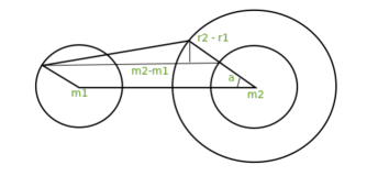
Figure 1.1. Illustration for $W_{2}$ distance computation between two circles $(m_{1},r_{1})$ and $(m_{2},r_{2})$.

$$W_{2}^{2}\big{(}(m_{1},r_{1}),(m_{2},r_{2})\big{)}$$

$$=\frac{1}{2\pi}\int_{0}^{2\pi}[(m_{2}-m_{1})-(r_{2}-r_{1})\cos(a)]^{2}+[(r_{2}-r_{1})\sin(a)]^{2}da$$

$$=(m_{2}-m_{1})^{2}+(r_{2}-r_{1})^{2}$$

Their $W_{2}^{2}$ barycenter is also a circle with mean $m=\frac{1}{n}\sum_{i=1}^{n}m_{i}$ and radius $r=\frac{1}{n}\sum_{i=1}^{n}r_{i}$. We refer to papers BinWas, PenWas, bc_coords_proj for an overview of the barycenters and related study.

$W_{1}$ barycenter in the previous example doesn’t have an explicit formula but we will show below that it has Gaussian approximation. It is well known that the center-of-mass in $l_{2}$ norm converges to a Gaussian random vector. As for the barycenter ($\widehat{\mu}$), it is also expected to have some Gaussian properties. For example, if the measures are Gaussian themselves or one-dimensional or circles set then the Gaussian approximation of the $W_{2}^{2}$ barycenter is proven in papers BinWas, g_was_clt. In circles set case the mean and radius converge to some Gaussian variables as a sum of independent observations according to Central Limit Theorem. In one-dimensional case, denoting distribution functions by $F_{i}(x)$

$$W_{2}^{2}(\mu_{1},\mu_{2})=\int_{0}^{1}|F_{1}^{-1}(s)-F_{2}^{-1}(s)|^{2}ds$$

one gets

$$\widehat{F}^{-1}(s)=\frac{1}{n}\sum_{i=1}^{n}F_{i}^{-1}(s)$$

In the case of Gaussian measures with zero mean and variances $\{S_{i}\}$

$$W_{2}^{2}(\mu_{1},\mu_{2})=\operatorname{tr}\{S_{1}\}+\operatorname{tr}\{S_{2}\}-2\operatorname{tr}\{(S_{2}^{1/2}S_{1}S_{2}^{1/2})^{1/2}\}$$

and for some non-random matrix $S_{*}$ (ref. LimitWasG) the corresponded barycenter variance is

$$\widehat{S}=\frac{1}{n}\sum_{i=1}^{n}(S_{*}^{1/2}S_{i}S_{*}^{1/2})^{1/2}+O(1/n)$$

In both last examples one deals with a mean of independent random variables. Being multiplied by $\sqrt{n}$ factor, they converge to a Gaussian variable (or to a Gaussian process in case of $\widehat{F}^{-1}(s)$ by Donsker’s Theorem). In general case it appears to be very difficult to reveal such convergence because the barycenter doesn’t have an explicit equation and it is an infinite-dimensional object. In order to handle with this difficulty we propose an approximation of the $W_{1}$ barycenter by a sum of independent variables using projection into Fourier basis and involve some novel results from statistical learning theory. The perspective of Fourier Analysis provides a suitable representation of the Wasserstein distance and it is already studied in the literature FouWas. Denote a range of size $p$ of the barycenter Fourier coefficients by

$$\widehat{\theta}_{p}=\mathcal{F}_{p}\left(\frac{d\widehat{\mu}(x)}{dx}\right),\quad\theta^{*}_{p}=\mathcal{F}_{p}\left(\frac{d\mu^{*}(x)}{dx}\right)$$

The first our result states that for some non-random matrix $\breve{D}$, independent random vectors $\{\xi_{i}\}$, and some depending on $p$ constant

$$\left\|\breve{D}\left(\widehat{\theta}_{p}-\theta^{*}_{p}\right)-\sum_{i=1}^{n}\xi_{i}\right\|=\frac{C(p)}{\sqrt{n}}$$

Further we show that for some Gaussian vector $Z$

$$W_{1}\left(\breve{D}(\widehat{\theta}_{p}-\theta^{*}_{p}),\,Z\right)=\frac{C(p)}{\sqrt{n}}$$

and $\forall z\in I\!\!R_{+}$:

$$\left|P\left(\|\breve{D}(\widehat{\theta}_{p}-\theta^{*}_{p})\|>z\right)-P\left(\|Z\|>z\right)\right|=\frac{C(p)}{\sqrt{n}}$$

Statistical Application: The last statement allows us to obtain the confidence region of parameter $\widehat{\theta}_{p}$ and describe the distribution inside the region. Besides, the bootstrap procedure validity LimitWas follows from our proof as well. If one samples $\|\breve{D}(\theta_{p}^{boot}-\widehat{\theta}_{p})\|$ using bootstrap it would be close by quantiles to the random variable $\|\breve{D}(\widehat{\theta}_{p}-\theta^{*}_{p})\|$, which also relates to the formation of the confidence region. In bc_coords_proj the authors demonstrate application of barycentric coordinates that allow to infer missing geometry of an input mesh using a set of 3D models. Recent article brule shows empirically that barycenters may be helpful as a loss function in unsupervised face landmarks detection task.

The Structure of this paper is the following. The main Theorems are in Section 2. Section 3 deals with independent parametric models and describes how one can approximate parameter deviations by a sum of independent random vectors $\{\xi_{i}\}$. In Section 4 we explore the barycenters model, compute derivatives of the Wasserstein distance using infimal convolution of support functions and check the required assumptions from the 3-rd Section. Section 5 contains some useful properties of the support functions. The final part, Gaussian approximation of the parameter $\widehat{\theta}_{p}$, is completed in Section 6, where we prove that $\{\xi_{i}\}$ is close to $Z$ by distribution.

2. The main result

Definition 2.1 (W-dual).

For two random variables $X$ and $Y\in\mathbb{R}^{\infty}$ with densities $\varphi_{X}$ and $\varphi_{Y}$ define Wasserstein distance in dual form as

$$W_{1}(\varphi_{X},\varphi_{Y})=\max_{\forall x:\|\nabla f(x)\|\leq 1}\{I\!\!Ef(X)-I\!\!Ef(Y)\}$$

where $\forall x:\|\nabla f(x)\|\leq 1$ means that function $f$ is $1$-Lipshits. Note that if $\pi(x,y)$ is a joint distribution with marginals $\varphi_{X}$ and $\varphi_{Y}$ then this definition is equivalent to the original (1.1), which follows from Kantorovich-Rubinstein duality KRdual.