END-TO-END BINAURAL SOUND LOCALISATION FROM THE RAW WAVEFORM

Abstract

A novel end-to-end binaural sound localisation approach is proposed which estimates the azimuth of a sound source directly from the waveform. Instead of employing hand-crafted features commonly employed for binaural sound localisation, such as the interaural time and level difference, our end-to-end system approach uses a convolutional neural network (CNN) to extract specific features from the waveform that are suitable for localisation. Two systems are proposed which differ in the initial frequency analysis stage. The first system is auditory-inspired and makes use of a gammatone filtering layer, while the second system is fully data-driven and exploits a trainable convolutional layer to perform frequency analysis. In both systems, a set of dedicated convolutional kernels are then employed to search for specific localisation cues, which are coupled with a localisation stage using fully connected layers. Localisation experiments using binaural simulation in both anechoic and reverberant environments show that the proposed systems outperform a state-of-the-art deep neural network system. Furthermore, our investigation of the frequency analysis stage in the second system suggests that the CNN is able to exploit different frequency bands for localisation according to the characteristics of the reverberant environment.

Index Terms—  Sound localisation, azimuth, end-to-end, convolutional neural networks, raw waveform.

1 Introduction

In the last decade, much effort has been spent towards the development of sound localisation systems. Classical approaches include estimation of the time difference of arrivals (TDOAs) between microphone pairs using the generalised cross-correlation (GCC) [1, 2], beamformer based models such as SRP-PHAT [3], and spectral estimation-based methods such as the multiple signal classification algorithm (MUSIC) [4]. More recently, localisation systems based on deep neural networks (DNNs) have shown promising performance. In [5], probabilistic neural networks were used to estimate the direction of arrival (DOA) in an indoor environment using GCC-based features. A similar scenario was studied in [6] which used a convolutional neural network (CNN) to predict speaker coordinates. Binaural cues are employed in [7], where the cross-correlation function (CCF) was used as features in a DNN to estimate the azimuth of a sound source with simulated head movement. CNN architectures were also used in [8, 9] using frequency-domain features such as the phase or the magnitude of the signal.

All of the approaches so far are based on hand-crafted features explicitly extracted from the waveform. Such a feature extraction process may lead to a loss of information which can affect the performance. Human listeners, on the other hand, are able to use waveforms from just two ears to reliably determine the location of a sound source [10]. It is well known that this ability is largely based on both binaural cues, such as the interaural time difference (ITD) and the interaural level difference (ILD), and monaural spectral cues created by direction-dependent filtering of the outer ears. However, it is less clear how these cues are seamlessly combined and processed by the auditory cortex for sound localisation [11].

Recently, much effort has been spent in the development of end-to-end systems for many audio applications. For example, a model for end-to-end automatic speech recognition (ASR) is proposed in [12], which combines localisation, beamforming, acoustic modelling and speech enhancement in a unified DNN. In audio generation, several end-to-end methods were proposed to directly generate waveforms from text [13, 14].

This paper proposes a novel end-to-end approach for sound localisation, referred to as WaveLoc. Instead of an explicit feature extraction stage, the proposed approach uses a CNN with a cascade of convolutional layers to implicitly extract features directly from the raw waveform for sound localisation. One of the key stages in the network is the frequency analysis, and two different approaches are investigated. The first approach is auditory-inspired and uses a convolutional layer based on the gammatone filterbank [15]. The gammatone filter is a widely-used model of auditory frequency analysis, with bandwidths set to reproduce human critical bandwidths [16]. In the second model, we adopt a standard convolutional layer which is intended to learn how to perform frequency analysis along with the training process of the entire network. After frequency analysis, further convolutional layers with 2-D kernels operates directly on the signals from both ears to extract features that are similar to the binaural cues used by the auditory system. The extracted features are finally concatenated and used as input to a DNN with fully connected layers, in order to map them to the corresponding source azimuth.

Our evaluation shows that the proposed WaveLoc systems are able to accurately estimate the azimuth of a sound source in the anechoic condition. However, the performance of the data-driven WaveLoc approach is poor in reverberant conditions when trained only on anechoic signals. This leads to a detailed investigation of the benefits of multi-conditional training (MCT), following which we are able to demonstrate robust performance of the wave-based approaches across a range of challenging reverberant conditions.

The rest of the paper is organised as follows. Section 2 presents the proposed end-to-end sound localisation framework, with a focus on two waveform-based approaches that differ in the frequency analysis stage. The experiment setups are described in Section 3 and results are presented with discussions in Section 4. Finally, Section 5 concludes the paper and makes suggestions for future work.

Fig. 1: The proposed end-to-end WaveLoc-GTF system using convolutional neural networks for binaural sound localisation.

2 System Description

2.1 Overview

The proposed end-to-end sound localisation approach is illustrated in Fig. 1. The convolutional neural network can be broadly divided into three stages: (i) a frequency analysis stage that takes the framed binaural ear signals as input, (ii) a feature extraction stage with a cascade of convolutional layers to extract suitable features for sound localisation, and (iii) a sound localisation stage based on several dense layers to perform sound localisation as a classification task.

The raw waveforms of the left and right ear signals, as indicated by ‘L’ and ‘R’ in Fig. 1, are directly used as inputs to the proposed CNNs. The ear signals are sampled at 16 kHz and framed with 20 ms window size with 10 ms overlap. In each frame the left and right channels are stacked together to form an input matrix of size $2\times 320$.

It is well established that the auditory system performs a frequency analysis that divides the ear signal into frequency bands, and then does analysis on the fine time signal in each band [17, 18]. Such processing has been shown to improve the robustness when exploited in a binaural sound localisation system, particularly in reverberant environments [19]. To simulate this operation, the first stage of the CNN performs a frequency analysis which filters the ear signals in the time domain with convolutional kernels.

Two frequency analysis strategies were investigated in this study. In the first system, named WaveLoc-GTF, the frequency analysis is performed by a convolution layer which is broadly based on a gammatone filterbank [15]. As shown in Fig. 1, the frequency analysis layer consists of a number of frequency channels. The following layers in each frequency channel elaborate upon the frequency analysis output, in order to extract frequency-dependent features. The second system, named WaveLoc-CONV imposes no constraint on frequency analysis. Instead, a convolutional layer with 1-D convolutional kernels is exploited to analyse frequency, with parameters learned from the data as part of the network training process.

In both systems, the frequency analysis is followed by a layer of 2-D convolutional kernels to extract features based on correlations of the left and the right channels. In WaveLoc-GTF these kernels are applied separately for each output of the gammatone filters, while in WaveLoc-CONV they are applied to the single frequency analysis layer. The correlation-based features are closely related to ITD and ILD cues, which are further elaborated by another convolutional layer with 1-D kernels in order to search for specific patterns that are related to the localisation task. Finally, the features produced by the convolutional layers are flattened and concatenated, before being passed to two dense layers. A softmax activation function is used in the output layer in order to perform sound localisation as a classification task.

2.2 WaveLoc-GTF

Fig. 1 illustrates the first proposed CNN: WaveLoc-GTF. As discussed, the frequency analysis is performed by a gammatone filter bank, which consists of 32 filters spanning between 70 and 7000 Hz with peak gain set to 0 dB. These filters are directly coded into non-trainable CNN kernels of size $1\times 320$, with a linear activation function. The gammatone impulse response is given by:

$$w[t]=at^{n-1}\cos(2{\pi}ft+\phi)e^{-2\pi bt}$$ (1)

where $t$ is time, $a$ is the amplitude, $f$ is the centre frequency, $\phi$ is the phase of the carrier, $n$ is the filter’s order, and $b$ is the filter’s bandwidth. In order to perform a time convolution, each filter is flipped in time so that the kernel operation is defined as:

$$y[t]=\sum_{m=-M}^{M}x[m]w[t-m]$$ (2)

where $x$ is the input signal, $w$ the weights of the filter, $t$ is the index of the actual value and $M$ is the filter length.

In each frequency band, the resulting feature maps share the same dimensions ($2\times 320$) of the input matrix. A normalisation layer is then applied which looks for the maximum absolute value across all the gammatone channels before dividing them by this value. Hence, the output feature values range between [-1,1], which are further processed with $1\times 2$ max pooling.

A separate stack of two further convolutional layers processes each normalised channel, searching for specific patterns related to localisation. The first convolutional layer has 2-D kernels of size $2\times 18$ and the second layer has a set of 1-D kernels of size $1\times 6$. Both convolutional layers are followed by $1\times 4$ max pooling and employ ReLU activation. Finally, the processed channels are concatenated. and fed into two fully connected dense layers. Each dense layer consists of 1024 hidden units with ReLU activation and a dropout rate of 0.5.

The output layer consists of 37 nodes corresponding to the 37 azimuth classes, with softmax activation.

2.3 WaveLoc-CONV

The neural architecture of the second system, WaveLoc-CONV, employs a single convolutional layer dedicated to frequency analysis. Its key difference from WaveLoc-GTF is that the frequency analysis of this model is learnt during the training process together with other parameters of the network. A convolutional layer with 64 1-D kernels of shape $1\times 256$ is employed as time domain filters for frequency analysis. It is reasonable to expect that the shape of a convolutional kernel directly trained on a raw waveform will be similar to all the sinusoidal components that form the waveform itself. In other words, the convolutional kernels are characterised by a set of sinusoidal functions, which lead to a particular frequency response of the kernel itself [12].

The convolutional layer is followed by $1\times 2$ max pooling with a linear activation function applied. As in WaveLoc-GTF, two more convolutional layers are employed to search for features suitable for localisation. However, instead of acting separately for each channel as in WaveLoc-GTF, they now jointly process all the output of the frequency analysis stage. The first of the two layers uses 64 2-D kernels of size $2\times 18$ to look for correlations between the left and right channels. The second uses 64 1-D kernels of size $1\times 6$. Both layers use the ReLu activation function and are followed by $1\times 4$ max pooling. Finally, the outputs are flattened and fed into a two fully-connected hidden layers with 1024 units each. The output layer uses softmax activation with 37 neurons.

The hyperparameters or both end-to-end architectures are chosen based on an optimisation process using a development dataset.

3 Evaluation

3.1 Binaural simulation

Binaural signals were simulated by convolving speech recordings with the Surrey binaural room impulse response (BRIR) database [20]. The Surrey BRIRs were captured using a Cortex head and torso simulator (HATS) in both anechoic and reverberant rooms. A total of 37 azimuth angles were used, ranging from [-90 °, 90 °] in steps of 5 °, where 0 ° is located exactly in front of the head. Four reverberant rooms were employed, denoted A–D. The reverberation time (T₆₀) and direct-to-reverberant ratio (DRR) of each room are listed in Table 1.

Table 1: Room characteristics of the Surrey BRIR database [20].

	Room A	Room B	Room C	Room D
$\mathrm{T}_{60}$ (s)	0.32	0.47	0.68	0.89
$\mathrm{DRR}$ ($\mathrm{d}\mathrm{B}$)	6.09	5.31	8.82	6.12

Speech signals belonging to the DARPA TIMIT database [21] were convolved with each BRIRs. The initial and final frames of each speech utterance were truncated if silence was present. The training dataset was obtained by randomly selecting 24 sentences per azimuth from the TIMIT training subset, while another 6 sentences composed the validation dataset. 15 more sentences per azimuth were selected from the TIMIT test subset to create the test dataset.

3.2 Experimental setup

For training the Adam optimiser with a learning rate of $1\mathrm{e}{-3}$ and a batch size of 128 samples was employed. The training process lasted for 50 epochs, but early stopping was applied if no improvement was observed on the validation set for more than 5 epochs. A decreasing learning rate was employed to improve training, being multiplied by 0.2 if no lower error was achieved after 2 epochs.

The networks were trained in two acoustic room conditions: (i) using anechoic signals only for training; (ii) multiconditional training, in which the networks were trained using data from all the reverberant rooms apart from the one used for test.

The evaluation results are reported based on chunks. Each chunk is 250 ms long (25 frames). The prediction made for each frame in a chunk is averaged to report a single azimuth location for the chunk. Chunk-based evaluation was adopted in order to avoid the issue that a speech signal typically includes short pauses where there is no directional sound source. The accuracy of the models was finally measured in terms of root mean square error (RMSE) given in degrees.

3.3 Baseline system

The baseline system is a state-of-the-art DNN-based localisation system using GCC-PHAT features as inputs [6, 22]. GCC-PHAT features are computed as the inverse transform of the frequency domain cross-correlation of two audio signals captured by a microphone pair. The binaural signals sampled at 16 kHz are framed at 20 ms, with 10 ms overlap. Since a distance of 18 cm occurs between the two microphones, the first 37 values are selected from the inverse transform. Unit variance and zero mean normalization is then applied. The baseline network consists of an input layer, two hidden layers of 1024 units each and an output layer of 37 classes. Dropout equal to 0.5 is applied after the two hidden layers. Softmax is selected as the activation function for the output layer, while a sigmoid activation function is used for the hidden units. All the hyperparameters were optimised using the development dataset.

4 Results and Discussion

4.1 Anechoic training

Table 2 shows results using systems trained in the anechoic condition. The best overall performance is achieved by the baseline GCC system. The proposed WaveLoc-GTF performed slightly worse compared to the baseline, while the localisation errors for WaveLoc-CONV were considerably larger across all reverberant conditions.

Table 2: Localisation RMSE results in degrees for the models trained in anechoic environment.

Room	Anechoic	A	B	C	D
Baseline	0.1 °	2.6 °	9.3 °	2.6 °	10.1 °
WaveLoc-GTF	0 °	9.1 °	10.7 °	1.6 °	10.5 °
WaveLoc-CONV	0 °	37.7 °	41.8 °	37.3 °	44.4 °

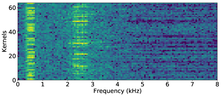
Fig. 2: Log-power spectra of the kernels in the first convolutional layer of WaveLoc-CONV when trained in the anechoic environment.

It appears that the WaveLoc-CONV system has a tendency for overfitting compared to the other two systems. Fig. 2 shows the log-power spectra of all the 64 kernels in the first convolutional layer in WaveLoc-CONV. It is clear that the kernels, when trained in the anechoic condition, act largely as a set of band pass filters, mostly enhancing the frequency bands between 300–600 Hz and between 2300–2800 Hz. It is widely known that binaural features such as ITDs are more reliable in the low frequency region below 1600 Hz while others such as ILDs become more robust in the high frequency region above 1600 Hz [10]. It is possible that the network extracts related binaural features which are most effective in these two bands for sound localisation in the anechoic condition. Such behaviour, however, failed to generalise to unseen reverberant conditions as these frequency bands could become unreliable due to reverberation.

The WaveLoc-GTF model, on the other hand, performs frequency analysis with the gammatone filterbank layer which forces the system to exploit all frequency bands and thus extract the most effective localisation features in each band.

4.2 Multiconditional training

It has been shown in the past that MCT can mitigate overfitting and increase the robustness of sound localisation in reverberant conditions [7, 23]. This can be done by adding either diffuse noise or reverberation to the training signals. In this study, a reverberant training approach was adopted as our preliminary experiments showed it to be more effective. Specifically, the anechoic training dataset was supplemented with reverberant versions by convolving it with various BRIRs. For each one of the four reverberant room under evaluation, all the remaining three were included for MCT.

Table 3: Localisation RMSE results in degrees using MCT.

Room	A	B	C	D
Baseline	2.7 °	3.3 °	3.1 °	5.2 °
WaveLoc-GTF	1.5 °	3.0 °	1.7 °	3.5 °
WaveLoc-CONV	1.7 °	2.3 °	1.4 °	2.4 °

Table 3 lists the results of all the models. The anechoic condition was excluded in this study, as all the models performed well even without MCT. All the models benefitted from MCT, especially the proposed WaveLoc models. The best overall performance in reverberant conditions is achieved by the WaveLoc-CONV model, which has an average localisation RMSE less than 3 °compared to over 30 °without MCT.

To investigate the effect of MCT on the convolutional kernels, we again plot the log-power spectra of all the 64 kernels in the first convolutional layers of the WaveLoc-CONV model. Only the plot for Room D is shown in Fig. 3 but plots for all the other rooms are similar. It can be seen that the first convolutional layer is now composed of a set of distributed bandpass filters emphasising mainly the 1500-4000 Hz range, with some kernels stretching up to 6–7 kHz. The low frequencies below 1500 Hz are less exploited by the WaveLoc-CONV model. It is interesting to notice that the data-driven model learns to use more high frequency cues in a reverberant environment, which suggests ILD become more useful than ITD. It is reasonable to expect that the ITD is more affected by reverberation, while the ILD, created by the head shadowing effect mainly for frequencies higher than 1600 Hz, is more robust to reverberation. Indeed, psychophysical cue-trading studies find that human listeners give ILD more weight than ITD when localising sounds in reverberant conditions [24].

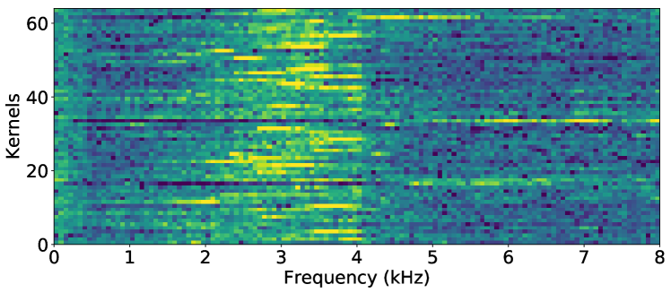
Fig. 3: Log-power spectra of the kernels in the first convolutional layer of WaveLoc-CONV when trained using MCT.

5 Conclusions

This paper described a new approach for localising a sound source directly from the waveform, by proposing two novel end-to-end CNN systems. Machine localisation systems typically employ hand-crafted features, such as the ITD and ILD. Such explicit feature extraction may limit the model performance since it implies a lossy transformation of the input signals. Instead, the proposed end-to-end approach employs a cascade of convolutional layers to extract features directly from the waveform, that are suitable for localisation in reverberant environments. When MCT was used across reverberant conditions, both end-to-end systems outperformed a state-of-the-art DNN system using conventional features.

Two CNN-based systems were introduced. The first system, WaveLoc-GTF, is inspired by the auditory system and employs a convolutional layer that is largely based on a gammatone filterbank. The second system, WaveLoc-CONV, employs a data-driven approach, where a convolutional layer with trainable 1-D kernels is dedicated for frequency analysis. Although the gammatone filterbank is in some sense more ‘principled’, since it approximates the filtering characteristics of the human auditory system, it does not work as well as a system that is trained (i.e., finds its own filters) across a number of reverberation conditions. One reason for this is that the system may elect to emphasise frequency regions during training that provide more robust cues to localisation.

Indeed, we found that when MCT was used, the WaveLoc-CONV model was better able to exploit features in the high frequency regions above 2 kHz, which tend to be less corrupted by reverberation. This mirrors findings from human perception suggesting that ILD (which is primarily available at high frequencies) is more robust than ITD when reverberation is present.

Future work will focus on improving the ability of end-to-end systems to generalise to unseen room conditions and multiple sources. Another possible direction is to combine sound identification with sound localisation within an end-to-end system [25]. Finally, we plan to conduct ‘psychophysical’ studies on trained networks in order to fully understand their underlying mechanisms, e.g. by using the cue trading protocol described in [24].

References

- [1] C. K. Knapp and G. C. Carter, “The generalized correlation method for estimation of time delay,” IEEE Trans. Acoust., Speech, Signal Process., vol. 24, no. 4, pp. 320–327, 1976.
- [2] M. S. Brandstein and H. F. Silverman, “A practical methodology for speech source localization with microphone arrays,” Computer Speech & Language, vol. 11, no. 2, pp. 91–126, 1997.
- [3] J. H. DiBiase, A high-accuracy, low-latency technique for talker localization in reverberant environments using microphone arrays, Ph.D. thesis, Brown University, 2000.
- [4] R. Schmidt, “Multiple emitter location and signal parameter estimation,” IEEE transactions on antennas and propagation, vol. 34, no. 3, pp. 276–280, 1986.
- [5] Y. Sun, J. Chen, C. Yuen, and S. Rahardja, “Indoor sound source localization with probabilistic neural network,” IEEE Transactions on Industrial Electronics, vol. 65, no. 8, pp. 6403–6413, 2018.
- [6] F. Vesperini, P. Vecchiotti, E. Principi, S. Squartini, and F. Piazza, “Localizing speakers in multiple rooms by using deep neural networks,” Computer Speech & Language, vol. 49, pp. 83–106, 2018.
- [7] N. Ma, T. May, and G. J. Brown, “Exploiting deep neural networks and head movements for robust binaural localisation of multiple sources in reverberant environments,” IEEE Trans. Audio, Speech, Lang. Process., vol. 25, no. 12, pp. 2444–2453, 2017.
- [8] S. Chakrabarty and E. Habets, “Multi-speaker localization using convolutional neural network trained with noise,” arXiv preprint arXiv:1712.04276, 2017.
- [9] S. Adavanne, S. Politis, J. Nikunen, and T. Virtanen, “Sound event localization and detection of overlapping sources using convolutional recurrent neural networks,” arXiv preprint arXiv:1807.00129, 2018.
- [10] J. Blauert, Spatial hearing - The psychophysics of human sound localization, The MIT Press, Cambridge, MA, USA, 1997.
- [11] Grothe B., Pecka M., and McAlpine D., “Mechanisms of sound localization in mammals,” Physiol. Rev., vol. 90, pp. 983–1012, 2010.
- [12] Tara N Sainath, Ron J Weiss, Kevin W Wilson, Bo Li, Arun Narayanan, Ehsan Variani, Michiel Bacchiani, Izhak Shafran, Andrew Senior, Kean Chin, et al., “Multichannel signal processing with deep neural networks for automatic speech recognition,” IEEE/ACM Transactions on Audio, Speech, and Language Processing, vol. 25, no. 5, pp. 965–979, 2017.
- [13] A. Van Den Oord, S. Dieleman, H. Zen, K. Simonyan, O. Vinyals, A. Graves, N. Kalchbrenner, A. W. Senior, and K. Kavukcuoglu, “Wavenet: A generative model for raw audio.,” in SSW, 2016, p. 125.
- [14] S. Mehri, K. Kumar, I. Gulrajani, R. Kumar, S. Jain, J. Sotelo, A. Courville, and Y. Bengio, “SampleRNN: An unconditional end-to-end neural audio generation model,” arXiv preprint arXiv:1612.07837, 2016.
- [15] R. D. Patterson, K. Robinson, J. Holdsworth, D. McKeown, C.Zhang, and M. H. Allerhand, “Complex sounds and auditory images,” Auditory Physiology and Perception, (Eds.) Y. Cazals, L. Demany, K.Horner, Pergamo, pp. 429–446, 1992.
- [16] D. L. Wang and G. J. Brown, Eds., Computational Auditory Scene Analysis: Principles, Algorithms and Applications, Wiley/IEEE Press, 2006.
- [17] G. Ehret, “Stiffness gradient along the basilar membrane as a basis for spatial frequency analysis within the cochlea,” The Journal of the Acoustical Society of America, vol. 64, no. 6, pp. 1723–1726, 1978.
- [18] W. Yost, “Structure of the inner ear and its mechanical response,” in Fundamentals of Hearing: An Introduction (5th edition), chapter 7, pp. 83–101. Brill, 2013.
- [19] N. Ma, J. A. Gonzalez, and G. J. Brown, “Robust binaural localization of a target sound source by combining spectral source models and deep neural networks,” IEEE Trans. Audio, Speech, Lang. Process., vol. 26, no. 11, pp. 2122–2131, 2018.
- [20] C. Hummersone, R. Mason, and T. Brookes, “Dynamic precedence effect modeling for source separation in reverberant environments,” IEEE Trans. Audio, Speech, Lang. Process., vol. 18, no. 7, pp. 1867–1871, 2010.
- [21] J. S. Garofolo, L. F. Lamel, W. M. Fisher, J. G. Fiscus, D. S. Pallett, and N. L. Dahlgren, “DARPA TIMIT Acoustic-phonetic continuous speech corpus CD-ROM,” National Inst. Standards and Technol. (NIST), 1993.
- [22] X. Xiao, S. Zhao, X. Zhong, D. L. Jones, E. Cheng, and H. Li, “A learning-based approach to direction of arrival estimation in noisy and reverberant environments,” in Acoustics, Speech and Signal Processing (ICASSP), 2015 IEEE International Conference on. IEEE, 2015, pp. 2814–2818.
- [23] T. May, S. van de Par, and A. Kohlrausch, “A probabilistic model for robust localization based on a binaural auditory front-end,” IEEE Trans. Audio, Speech, Lang. Process., vol. 19, no. 1, pp. 1–13, 2011.
- [24] T. M. Nguyen, The effects of target spectrum, noise, and reverberation on auditory cue weighting in sound localization, Ph.D. thesis, University of Western Ontario, 2014.
- [25] E. Çakir and T. Virtanen, “End-to-end polyphonic sound event detection using convolutional recurrent neural networks with learned time-frequency representation input,” in 2018 International Joint Conference on Neural Networks (IJCNN), July 2018, pp. 1–7.