Statistical Analysis of Some Evolution Equations Driven by Space-Only Noise

Abstract.

We study the statistical properties of stochastic evolution equations driven by space-only noise, either additive or multiplicative. While forward problems, such as existence, uniqueness, and regularity of the solution, for such equations have been studied, little is known about inverse problems for these equations. We exploit the somewhat unusual structure of the observations coming from these equations that leads to an interesting interplay between classical and non-traditional statistical models. We derive several types of estimators for the drift and/or diffusion coefficients of these equations, and prove their relevant properties.

1. Introduction

While the forward problems, existence, uniqueness, and regularity of the solution, for stochastic evolution equations have been extensively studied over the past few decades (cf. [13, 14] and references therein), the literature on statistical inference for SPDEs is, relatively speaking, limited. We refer to the recent survey [3] for an overview of the literature and existing methodologies on statistical inference for parabolic SPDEs. In particular, little is known about the inverse problems for stochastic evolutions equations driven by space-only noise, and the main goal of this paper is to investigate the parameter estimation problems for such equations. The somewhat unusual structure of the space-only noise exhibits interesting statistical inference problems that stay at the interface between classical and non-traditional statistical models. We consider two classes of equations, corresponding to two types of noise, additive and multiplicative. As an illustration, let us take a heat equation

$$u_{t}=\boldsymbol{\Delta}u,\quad t>0,$$

on some domain and with some initial data, and where $\boldsymbol{\Delta}$ denotes the Laplacian operator. Customarily, a random perturbation to this equation can be additive

(1.1) $$u_{t}=\boldsymbol{\Delta}u+\dot{W},$$

representing a random heat source, or multiplicative

(1.2) $$u_{t}=u_{xx}+u\dot{W},$$

representing a random potential. In the case of space-dependent noise and pure point spectrum of the Laplacian $\boldsymbol{\Delta}$, one can also consider a shell version of (1.2):

(1.3) $$u_{t}=\boldsymbol{\Delta}u+\sum_{k}u_{k}\xi_{k}h_{k}(x),$$

in which $\{h_{k},\ k\geq 1\}$ are the normalized eigenfunctions of the Laplacian, $u_{k}=(u,h_{k}),\ \ \xi_{k}=\dot{W}(h_{k})$. Similar decoupling of the Fourier modes is used to study nonlinear equations in fluids mechanics, both deterministic [6, Section 8.7] and stochastic [7, 5]; the term “shell model” often appears in that context.

Our objective is to study abstract versions of (1.3) and (1.1) with unknown coefficients:

(1.4) $$\dot{u}+\theta Au=\sigma\sum_{k=1}^{\infty}q_{k}u_{k}h_{k}\xi_{k},$$

and

(1.5) $$\dot{u}+\theta Au=\sigma\dot{W}^{Q},$$

where

• $A$ is a linear operator in a Hilbert space $H$;

• $\{h_{k}\}_{k\in\mathbb{N}}\subset H$ are the normalized eigenfunctions of $A$ that form a complete orthonormal system in $H$, with corresponding eigenvalues $\mu_{k}>0$, $k\in\mathbb{N}$;

• $q_{k}>0,\ k\in\mathbb{N}$, are known constants;

• $\theta>0$, $\sigma>0$ are unknown numbers (parameters of interest);

• $\xi_{k},\ k\in\mathbb{N}$, are independent and identically distributed (i.i.d.) standard normal random variables on the underlying probability space $(\Omega,\mathcal{F},\mathbb{P})$ and $\dot{W}^{Q}=\sum_{k=1}^{\infty}q_{k}\xi_{k}h_{k}$;

• $u_{k}=u_{k}(t)=(u,h_{k})_{H}$, $t\in[0,T],k\in\mathbb{N}$.

In each case, the solution is defined as

(1.6) $$u(t)=\sum_{k=1}^{\infty}u_{k}(t)h_{k},$$

with

(1.7) $$u_{k}(t)=u_{k}(0)\exp\Big{(}-(\theta\mu_{k}-\sigma q_{k}\xi_{k})t\Big{)}$$

for (1.4), and

(1.8) $$u_{k}(t)=u_{k}(0)e^{-\theta\mu_{k}t}+\frac{\sigma q_{k}}{\theta\mu_{k}}\left(1-e^{-\theta\mu_{k}t}\right)\xi_{k}$$

for (1.5). For both models (1.4) and (1.5), we assume that the observations are available in the Fourier space, namely, the observer measures the values of the Fourier modes $u_{k}(t)$, continuously in time for $t\in[0,T]$. In addition, for (1.5) we also consider statistical experiment when the observations are performed in physical space. The main results of this paper are summarized as follows:

1. For equation (1.4), knowledge of all $\mu_{k}$ is required; then, under some additional technical assumptions, the problem of joint estimation of $\theta$ and $\sigma$, using measurements in the Fourier space, leads to statistical experiment with LAN (local asymptotic normality) and several other regularity properties. Consequently, we prove strong consistency and asymptotic normality of maximum likelihood estimators (MLE) and Bayesian estimators for $\theta$ and $\sigma$; see Section 2.

2. For equation (1.5), the values of $\theta\mu_{k}$ can be determined exactly from the observations of $u_{k}(t)$ at two or three time points; estimation of $\sigma$ is then reduced to estimation of variance in a normal population with known mean; see Section 3.1. Using special structure of the solution of (1.5), and assuming zero initial conditions, and $q_{k}=1$, we derive consistent and asymptotically normal estimators of $\theta$ and $\sigma$, assuming measurements in the physical domain; see Section 3.2.

In Section 4, we present several illustrative examples, while Section 5 is dedicated to some numerical experiments that exemplify the theoretical results of the paper.

Throughout the paper, given two sequences of numbers $\{a_{n},\ n\geq 1\}$ and $\{b_{n},\ n\geq 1\}$, we write $a_{n}\sim b_{n}$ if there exists a positive number $c$ such that $\lim_{n\to\infty}a_{n}/b_{n}=c$.

2. The Shell Model

In this section we study the stochastic evolution equation (1.4), starting with the existence and uniqueness of the solution, and continuing with parameter estimation problem for $\theta$ and $\sigma$ within the LAN framework of [9]. For better comparison with existing results, such as [1] and [8], we consider a slightly more general version of (1.4):

(2.1) $$\dot{u}+(\theta A+A_{0})u=\sum_{k=1}^{\infty}(\sigma q_{k}+p_{k})u_{k}\xi_{k}h_{k},\ \ t>0,$$

with known $q_{k}>0,\ p_{k}\geq 0$ and the operators $A$ and $A_{0}$ such that

(2.2) $$Ah_{k}=\mu_{k}h_{k},\ A_{0}h_{k}=\nu_{k}h_{k},$$

and the real numbers $\mu_{k},\nu_{k}$ are known. The numbers $\theta$ and $\sigma$ are unknown and belong to an open set $\Theta\subseteq\mathbb{R}\times(0,+\infty)$.

The solution of (2.1) is defined by (1.6), with

(2.3) $$u_{k}(t)=u_{k}(0)\exp\Big{(}-(\theta\mu_{k}+\nu_{k})t+(\sigma q_{k}+p_{k})\xi_{k}\,t\Big{)}.$$

Theorem 2.1.

Assume that $u(0)\in H$, $u_{k}(0)\not=0$, $k\geq 1$, and there exists a real number $C^{*}$ such that for all $(\theta,\sigma)\in\Theta$ and $k\geq 1$,

$$\theta\mu_{k}+\nu_{k}>C_{*}.$$

If

(2.4) $$\lim_{k\to\infty}\frac{(\sigma q_{k}+p_{k})^{2}}{\theta\mu_{k}+\nu_{k}}=0,$$

for all $(\theta,\sigma)\in\Theta$, then $u(t)\in L_{2}(\Omega;H)$ for all $t>0$ and $\mathbb{E}\|u(t)\|_{H}^{2}\leq C(t,\theta,\sigma)\|u(0)\|_{H}^{2}$.

If there exist $T>0$ and $\bar{C}_{T}\geq 0$ such that

(2.5) $$\Big{(}T(\sigma q_{k}+p_{k})^{2}-4(\theta\mu_{k}+\nu_{k})\Big{)}\leq 2\bar{C}_{T},$$

for all $k\geq 1$ and $(\theta,\sigma)\in\Theta$, then $u(t)\in L_{2}(\Omega;H)$ for all $t\in[0,T]$ and $\mathbb{E}\|u(t)\|_{H}^{2}\leq\|u(0)\|_{H}^{2}\,e^{T\bar{C}_{T}}$.

Proof.

By (2.3),

$$\mathbb{E}u_{k}^{2}(t) =u_{k}^{2}(0)\exp\left(-2(\theta\mu_{k}+\nu_{k})t+\frac{(\sigma q_{k}+p_{k})^{2}t^{2}}{2}\right)$$

(2.6) $$=u_{k}^{2}(0)\exp\left(-2t(\theta\mu_{k}+\nu_{k})\left(1-\frac{(\sigma q_{k}+p_{k})^{2}t}{4(\theta\mu_{k}+\nu_{k})}\right)\right)$$

(2.7) $$=u_{k}^{2}(0)\left(\frac{t}{2}\Big{(}(\sigma q_{k}+p_{k})^{2}t-4(\theta\mu_{k}+\nu_{k})\Big{)}\right).$$

If (2.4) holds, then, for every $t>0$, there exists $k=k(t)$ such that, for all $k>k(t)$,

$$1-\frac{(\sigma q_{k}+p_{k})^{2}t}{4(\theta\mu_{k}+\nu_{k})}>\frac{1}{2},$$

and then (2.6) implies

$$\mathbb{E}u_{k}^{2}(t)\leq u_{k}^{2}(0)\,e^{-C_{*}t},\ \ k>k(t),$$

concluding the proof.

If (2.5) holds, then (2.7) implies that, for all $t\in[0,T]$ and $k\geq 1$,

$$\mathbb{E}u_{k}^{2}(t)\leq u_{k}^{2}(0)\,e^{T\bar{C}_{T}},$$

concluding the proof. $\Box$

In what follows, we assume, with no loss of generality, that $C_{*}=0$.

Define

$$Y_{k}=\frac{1}{t}\ln\frac{u_{k}(t)}{u_{k}(0)},\quad k=1,\dots,N.$$

Then, for each $t>0$, the random variable $Y_{k}$ is Gaussian with mean $-(\theta\mu_{k}+\nu_{k})$ and variance $(\sigma q_{k}+p_{k})^{2}$, and the random variables $Y_{1},\ldots,Y_{N}$ are independent.

We consider $\theta$ and $\vartheta=\sigma^{2}$ as the two unknown parameters. The corresponding likelihood function becomes

(2.8) $$L_{N}(\theta,\vartheta)=\exp\left(-\frac{N}{2}\ln(2\pi)-\sum_{k=1}^{N}\ln(\sqrt{\vartheta}\,q_{k}+p_{k})-\frac{1}{2}\sum_{k=1}^{N}\frac{(Y_{k}+\theta\mu_{k}+\nu_{k})^{2}}{(\sqrt{\vartheta}\,q_{k}+p_{k})^{2}}\right).$$

Direct computations produce the Fisher information matrix

(2.11) $$I_{N} =\left(\begin{array}[]{cc}\Psi_{N}(\vartheta)&0\\ 0&\Phi_{N}(\vartheta)\end{array}\right),\ \ \ {\rm where}$$

(2.12) $$\Psi_{N}(\vartheta) =\sum_{k=1}^{N}\frac{\mu_{k}^{2}}{(\sqrt{\vartheta}\,q_{k}+p_{k})^{2}},\ \ \Phi_{N}(\vartheta)=\frac{1}{2}\sum_{k=1}^{N}\frac{q_{k}^{2}}{(\vartheta\,q_{k}+\sqrt{\vartheta}\,p_{k})^{2}}.$$

Note that if $p_{k}=0$ for all $k$, then $\Phi_{N}(\vartheta)=N/(2\sigma^{4})$. More generally, if

$$\lim_{k\to\infty}\frac{p_{k}}{q_{k}}=c_{pq}\in[0,+\infty),$$

then $\Phi_{N}\sim N$.

Proposition 2.2.

If $\Theta=\mathbb{R}\times(0,+\infty)$ and $p_{k}=0$ for all $k\geq 1$, then the joint maximum likelihood estimator of $(\theta,\vartheta)$ is

(2.13) $$\hat{\theta}_{N}=-\frac{\sum_{k=1}^{N}(\mu_{k}Y_{k}+\mu_{k}\nu_{k})/q_{k}^{2}}{\sum_{k=1}^{N}(\mu_{k}/q_{k})^{2}},\ \ \hat{\vartheta}_{N}=\frac{1}{N}\sum_{k=1}^{N}\frac{(Y_{k}+\hat{\theta}_{N}\mu_{k}+\nu_{k})^{2}}{q_{k}^{2}}.$$

While (2.13) follows by direct computation, a lot of extra work is required to investigate the basic properties of the estimator, such as consistency and asymptotic normality, and it still will not be clear how the estimator compares with other possible estimators, for example, Bayesian. Moreover, when $p_{k}\not=0$, no closed-form expressions for $\hat{\theta}_{N}$ and $\hat{\vartheta}_{N}$ can be found.

As a result, the main object of study becomes the local likelihood ratio

(2.14) $$Z_{N,\boldsymbol{\theta}}(\boldsymbol{x})=\frac{L_{N}(\theta(s),\vartheta(\tau))}{L_{N}(\theta,\vartheta)},\ \ \boldsymbol{\theta}=(\theta,\vartheta),\ \boldsymbol{x}=(s,\tau),$$

with

$$\theta(s)=\theta+\frac{s}{\sqrt{\Psi_{N}(\vartheta)}},\ \ \vartheta(\tau)=\vartheta+\frac{\tau}{\sqrt{\Phi_{N}(\vartheta)}}.$$

Then various properties of the maximum likelihood and Bayesian estimators, including consistency, asymptotic normality, and optimality, can be established by analyzing the function $Z_{N,\boldsymbol{\theta}}$; see [9, Chapters I–III].

Definition 2.3.

The function $Z_{N,\boldsymbol{\theta}}$ is called regular if the following conditions are satisfied.

1. For every compact set $K\subset\Theta$ and sequences $\boldsymbol{\theta}_{N}=(\theta_{N},\vartheta_{N})$, $\boldsymbol{\theta}_{N}(\boldsymbol{x}_{N})=\big{(}\theta_{N}(s_{N}),\vartheta_{N}(\tau_{N})\big{)}$ in $K$ with $\lim_{N\to\infty}(s_{N},\tau_{N})=(s,\tau)$, the representation

   (2.15) $$Z_{N,\boldsymbol{\theta}_{N}}(s_{N},\tau_{N})=\exp\left(s\eta_{N}+\tau\zeta_{N}-\frac{s^{2}}{2}-\frac{\tau^{2}}{2}+\varepsilon_{N}(\boldsymbol{\theta}_{N},\boldsymbol{x}_{N})\right),$$

   holds, so that, as $N\to\infty$, the random vector $(\eta_{N},\zeta_{N})$ converges in distribution to a standard bi-variate Gaussian vector and the random variable $\varepsilon_{N}(\boldsymbol{\theta}_{N},\boldsymbol{x}_{N})$ converges in probability to zero.

2. For every $\vartheta>0$,

   (2.16) $$\lim_{N\to\infty}\Psi_{N}(\vartheta)=\lim_{N\to\infty}\Phi_{N}(\vartheta)=+\infty.$$

3. To state the other two conditions, define

   $$U_{N}(\boldsymbol{\theta})=\big{\{}(s,\tau)\in\mathbb{R}^{2}:(\theta+s\Psi_{N}^{-1/2},\vartheta+\tau\Phi_{N}^{-1/2})\in\Theta\big{\}}.$$

4. For every compact $K\subset\Theta$, there exist positive numbers $a$ and $B$ such that, for all $N\geq 1$ and $R>0$,

   (2.17) $$\sup_{\boldsymbol{\theta}\in K}\sup_{\scriptsize{\begin{array}[]{c}\boldsymbol{x}\in U_{N}(\boldsymbol{\theta}),\,\boldsymbol{y}\in U_{N}(\boldsymbol{\theta}),\\ |\boldsymbol{x}|<R,\,|\boldsymbol{y}|<R\end{array}}}|\boldsymbol{x}-\boldsymbol{y}|^{-4}\ \mathbb{E}\Big{|}Z^{1/8}_{N,\boldsymbol{\theta}}(\boldsymbol{x})-Z^{1/8}_{N,\boldsymbol{\theta}}(\boldsymbol{y})\Big{|}^{8}\leq B(1+R^{a}).$$

5. For every compact set $K\subset\Theta$ and every $p>0$, there exists an $N_{0}=N_{0}(K,p)$ such that

   (2.18) $$\sup_{\boldsymbol{\theta}\in K}\sup_{N>N_{0}}\sup_{\boldsymbol{x}\in U_{N}(\boldsymbol{\theta})}|\boldsymbol{x}|^{p}\ \mathbb{E}Z^{1/2}_{N,\boldsymbol{\theta}}(\boldsymbol{x})<\infty.$$

Conditions R1–R4 are natural modifications of conditions N1–N4 from [9, Section III.1] to our setting. In particular, R1 is known as uniform local asymptotic normality. Note that, in R3, there is nothing special about the numbers 4 and 8 except that

1. The smaller of the two numbers should be bigger than the dimension of the parameter space (cf. [9, Theorem III.1.1]);

2. In the setting (2.8), (2.14), the larger number should be at least twice as big as the smaller number, which is related to the square root function connecting variance and standard deviation.

The next result illustrates the importance of regularity.

Theorem 2.4.

Assume that the function $Z_{N,\boldsymbol{\theta}}$ is regular. Then

1. The joint MLE $(\hat{\theta}_{N},\hat{\vartheta}_{N})$ of $(\theta,\vartheta)$ is consistent and asymptotically normal with rate $I_{N}^{1/2}$, that is, as $N\to\infty$, $\big{(}\sqrt{\Psi_{N}(\vartheta)}(\hat{\theta}_{N}-\theta),\sqrt{\Phi_{N}(\vartheta)}(\hat{\vartheta}_{N}-\vartheta)\big{)}$ converges in distribution to a standard bivariate Gaussian random vector. The estimator is asymptotically efficient with respect to loss functions of polynomial growth and, with $\eta_{N}$ and $\zeta_{N}$ from (2.15),

   $$\lim_{N\to\infty}\Big{(}\sqrt{\Psi_{N}(\vartheta)}\,(\hat{\theta}_{N}-\theta)-\eta_{N}\Big{)}=0,\ \ \lim_{N\to\infty}\Big{(}\sqrt{\Phi_{N}(\vartheta)}\,(\hat{\vartheta}_{N}-\vartheta)-\zeta_{N}\Big{)}=0,$$

   in probability.

2. Every Bayesian estimator $(\tilde{\theta}_{N},\tilde{\vartheta}_{N})$ corresponding to an absolutely continuous prior on $\Theta$ and a loss function of polynomial growth is consistent, asymptotically normal with rate $I_{N}^{1/2}$, asymptotically efficient with respect to loss functions of polynomial growth, and

   $$\lim_{N\to\infty}\sqrt{\Psi_{N}(\vartheta)}\,\big{(}\hat{\theta}_{N}-\tilde{\theta}_{N}\big{)}=0,\ \ \lim_{N\to\infty}\sqrt{\Phi_{N}(\vartheta)}\,\big{(}\hat{\vartheta}_{N}-\tilde{\vartheta}_{N}\big{)}=0$$

   in probability.

Proof.

The MLE is covered by the results of [9, Section III.1]. The Bayesian estimators are covered by the results of [9, Section III.2]. $\Box$

Accordingly, our objective is to determine the conditions on the sequences $\mu_{k},\nu_{k},q_{k},p_{k}$ so that the function $Z_{N,\boldsymbol{\theta}}$ defined by (2.14) is regular.

Theorem 2.5.

Assume that

(2.19) $$\sum_{k=1}^{\infty}\frac{\mu_{k}^{2}}{(q_{k}+p_{k})^{2}}=+\infty,$$

(2.20) $$\sum_{k=1}^{\infty}\frac{q_{k}^{2}}{(q_{k}+p_{k})^{2}}=+\infty.$$

Then the function $Z_{N,\boldsymbol{\theta}}$ is regular.

Proof.

To verify condition R1 from Definition 2.3, write

$$w_{k,N}=\sqrt{\vartheta_{N}}\,q_{k}+p_{k},\ \ \ \xi_{k,N}=\frac{Y_{k}+\theta_{N}\,\mu_{k}+\nu_{k}}{w_{k,N}}.$$

Direct computations show that (2.15) holds with

(2.21) $$\eta_{N}=-\frac{1}{\sqrt{\Psi_{N}(\vartheta_{N})}}\sum_{k=1}^{N}\frac{\mu_{k}\xi_{k,N}}{w_{k,N}},\ \ \ \zeta_{N}=\frac{1}{\sqrt{2\vartheta_{N}\,\Phi_{N}(\vartheta_{N})}}\sum_{k=1}^{N}\frac{q_{k}}{w_{k,N}}\,\frac{\xi_{k,N}^{2}-1}{\sqrt{2}},$$

and $\varepsilon_{N}(\boldsymbol{\theta}_{N},\boldsymbol{x}_{N})$ is a sum of

$$\varrho_{N}=\frac{1}{2\Phi_{N}(\vartheta_{N})}\sum_{k=1}^{N}\frac{\xi^{2}_{k,N}q_{k}^{2}}{\vartheta_{N}\,w_{k,N}^{2}}\ -\ 1$$

and several remainder terms coming from various Taylor expansions. By (2.20), $\lim_{N\to\infty}\varrho_{N}=0$ with probability one, uniformly on compact subsets of $\Theta$; cf. [16, Theorem IV.3.2]. Convergence to zero of the remainder terms is routine.

Next, let $\mathcal{H}_{q}$ be the $q$-the homogeneous chaos space generated by $\{\xi_{k,N},\ k=1,\ldots,N\}$. Then equalities (2.21) imply $\eta_{N}\in\mathcal{H}_{1}$, $\zeta_{N}\in\mathcal{H}_{2}$, $\mathbb{E}\eta_{N}^{2}=\mathbb{E}\zeta_{N}^{2}=1$, $\mathbb{E}(\eta_{N}\zeta_{N})=0$, and

$$\lim_{N\to\infty}\mathbb{E}\big{(}\eta_{N}^{2}+\zeta_{N}^{2}\big{)}^{2}=8,$$

uniformly in $(\theta_{N},\vartheta_{N})$. By [15, Theorem 1.1], it follows that $(\eta_{N},\zeta_{N})$ converges in distribution to a standard bi-variate Gaussian vector and the convergence is uniform in $(\theta_{N},\vartheta_{N})$. Condition R1 is now verified.

Assumptions (2.19) and (2.20) imply R2.

To simplify the rest of the proof, define

$$w_{k} =\sqrt{\vartheta}\,q_{k}+p_{k},\ \ \ w_{k}(\tau)=\sqrt{\vartheta(\tau)}\,q_{k}+p_{k},\ \ \ \xi_{k}=\frac{Y_{k}+\theta\,\mu_{k}+\nu_{k}}{w_{k}},$$

$$a_{k} =\frac{1}{2}\left(1-\frac{w_{k}^{2}}{w_{k}^{2}(\tau)}\right),\ \ \ b_{k}=\frac{w_{k}\mu_{k}}{\sqrt{\Psi_{N}}\,w_{k}^{2}(\tau)}\,s,$$

so that

(2.22) $$Z_{N,\boldsymbol{\theta}}(\boldsymbol{x})=\prod_{k=1}^{N}\left(\frac{w_{k}}{w_{k}(\tau)}\right)\exp\left(-\frac{s^{2}}{2\Psi_{N}}\sum_{k=1}^{N}\frac{\mu_{k}^{2}}{w_{k}^{2}(\tau)}\right)\exp\left(\sum_{k=1}^{N}\big{(}a_{k}\xi_{k}^{2}-b_{k}\xi_{k}\big{)}\right).$$

To verify R3, let

$$G_{N}(\boldsymbol{x})=Z^{1/8}_{N,\boldsymbol{\theta}}(\boldsymbol{x}).$$

This is a smooth function of $s$ and $w_{k}(\tau)$, whereas each function $\tau\mapsto w_{k}(\tau)$ is Hölder continuous of order $1/2$: if $N$ is small compared to $R$, then $\vartheta+\tau/\sqrt{\Phi_{N}}$ can be arbitrarily close to zero. By the chain rule, we conclude that R3 hods for every fixed $N$. It remains to verify R3 uniformly in $N$ for every fixed $K$ and $R$, and therefore we will assume from now on that $N$ is sufficiently large, and, in particular, $\vartheta+\tau/\sqrt{\Phi_{N}}$ is uniformly bounded away from zero.

By the mean value theorem,

$$|G_{N}(\boldsymbol{x})-G_{N}(\boldsymbol{y})|\leq R^{1/2}\sqrt{|\boldsymbol{x}-\boldsymbol{y}|}\ |\nabla G_{N}(\boldsymbol{x}^{*})|$$

and $\nabla G_{N}(\boldsymbol{x})=H_{N}(\boldsymbol{x})G_{N}(\boldsymbol{x})$, where the two-dimensional random vector $H_{N}$ satisfies $\sup_{N}\mathbb{E}|H_{N}|^{q}<\infty$ for every $q>0$. By the Hölder inequality,

$$\mathbb{E}\big{|}H_{N}(\boldsymbol{x})G_{N}(\boldsymbol{x})\big{|}^{8}\leq\Big{(}\mathbb{E}\big{|}H_{N}|^{8(1+\varepsilon)/\varepsilon}\Big{)}^{\varepsilon/(1+\varepsilon)}\Big{(}\mathbb{E}Z_{N,\boldsymbol{\theta}}^{1+\varepsilon}(\boldsymbol{x})\Big{)}^{1/(1+\varepsilon)},\ \varepsilon>0.$$

It follows from (2.22) that, for every $K$ and $R$, there is an $\varepsilon>0$ such that

$$\sup_{\boldsymbol{\theta}\in K}\sup_{\boldsymbol{x}\in U_{N}(\boldsymbol{\theta}),\,|\boldsymbol{x}|<R}\mathbb{E}Z_{N,\boldsymbol{\theta}}^{1+\varepsilon}(\boldsymbol{x})<B(K,R,\varepsilon),\ N>N_{0}(\varepsilon).$$

Condition R3 is now verified.

To verify R4, note that, for a standard Gaussian random variable $\xi$,

$$\mathbb{E}e^{a\xi^{2}-b\xi}=e^{-b^{2}/(4a)}\mathbb{E}e^{a(\xi-(b/2a))^{2}}=(1-2a)^{-1/2}e^{b^{2}/(2-4a)};$$

cf. [13, Proposition 6.2.31]. Then

$$\mathbb{E}Z_{N,\boldsymbol{\theta}}^{1/2}(\boldsymbol{x})=\left[\prod_{k=1}^{N}\left(\frac{2w_{k}w_{k}(\tau)}{w_{k}^{2}+w^{2}_{k}(\tau)}\right)^{1/2}\right]\exp\left(-\frac{s^{2}}{4\Psi_{N}}\sum_{k=1}^{N}\frac{\mu_{k}^{2}}{w_{k}^{2}+w^{2}_{k}(\tau)}\right).$$

To study $\big{(}|s|^{2}+|\tau|^{2}\big{)}^{p/2}\mathbb{E}Z_{N,\boldsymbol{\theta}}^{1/2}(\boldsymbol{x})$, denote by $C$ a number that does not depend on $N$ and $\boldsymbol{x}=(s,\tau)$; the value of $C$ can be different in different places. For $p>0,\ r>0$,

$$|s|^{p}e^{-rs^{2}}\leq\left(\frac{p}{2r}\right)^{p/2},$$

so that

$$|s|^{p}\exp\left(-\frac{s^{2}}{4\Psi_{N}}\sum_{k=1}^{N}\frac{\mu_{k}^{2}}{w_{k}^{2}+w^{2}_{k}(\tau)}\right) \leq C\left(\frac{\Psi_{N}}{\sum_{k=1}^{N}\mu_{k}^{2}/(w_{k}^{2}+w_{k}^{2}(\tau))}\right)^{p/2}$$

$$\leq C\big{(}\max(1,\tau)\big{)}^{p/2};$$

the last inequality follows from the definitions of $\Psi_{N}$ and $w_{k}^{2}(\tau)$. Writing

$$F_{N}(\tau)=|\tau|^{q}\prod_{k=1}^{N}\left(\frac{2w_{k}w_{k}(\tau)}{w_{k}^{2}+w^{2}_{k}(\tau)}\right)^{1/2},$$

the objective becomes to show that, for fixed $q>0$ and all sufficiently large $N$,

$$\max_{\tau>-\vartheta\sqrt{\Phi_{N}(\vartheta)}}F_{N}(\tau)<\infty,$$

which, in turn, follows by noticing that

$$\arg\max_{\tau>-\vartheta\sqrt{\Phi_{N}(\vartheta)}}F_{N}(\tau)=2\sqrt{q}+O\Big{(}\Phi^{-1/2}_{N}(\vartheta)\Big{)},\ N\to\infty,$$

and

$$\lim_{N\to\infty}F_{N}(2\sqrt{q})=(4q)^{q/2\,}e^{-q/2}.$$

Condition R4 is now verified, and Theorem 2.5 is proved. $\Box$

Taking $\mu_{k}=q_{k}=1,\ \nu_{k}=p_{k}=0$, we recover the familiar problem of joint estimation of mean and variance in a normal population. Because the Fisher information matrix is diagonal, violation of one of the conditions of the theorem still leads to a regular statistical model for the other parameter. For example, if (2.19) holds but (2.20) does not, then $\sigma$ is not identifiable, but $\theta$ is, and the local likelihood ratio $Z_{N,\theta}(s)=Z_{N,\boldsymbol{\theta}}(s,0)$ is regular, as a function of one variable.

Conditions (2.4) and (2.19) serve different purposes: (2.4) ensures that (2.1) has a global-in-time solution in $H$, whereas (2.19) implies regularity of the estimation problem for $\theta$ based on the observations (multi-channel model) $u_{k}$, $k=1,\ldots,N,\ N\to\infty.$ In general, (2.4) and (2.19) are not related: with $\theta=1,\ \mu_{k}=1,\ \nu_{k}=k^{4},\ q_{k}=k,\ p_{k}=0$, condition (2.4) holds, but (2.19) does not; taking $\theta=1,\ \mu_{k}=k^{2},\ q_{k}=k^{3/2},\ \nu_{k}=p_{k}=0,$ we satisfy (2.19) but not (2.4) [and not even (2.5)], and the resulting multi-channel model, while regular in statistical sense, does not correspond to any stochastic evolution equation.

Condition (2.20) means that the numbers $p_{k}$ are not too big compared to $q_{k}$; for example,

(2.23) $$\limsup_{k\to\infty}\frac{p_{k}}{\sqrt{k}\,q_{k}}<+\infty$$

is sufficient for (2.20) to hold.

By a theorem of Kakutani [10], (2.19) is equivalent to singularity of the measures

(2.24) $$\prod_{k\geq 1}\mathcal{N}\big{(}-(\theta\mu_{k}+\nu_{k}),(\sigma q_{k}+p_{k})^{2}\big{)}$$

on $\big{(}\mathbb{R}^{\infty},\mathcal{B}(\mathbb{R}^{\infty})\big{)}$ for different values of $\theta$, and (2.20) is equivalent to singularity of the measures (2.24) on $(\mathbb{R}^{\infty},\mathcal{B}(\mathbb{R}^{\infty}))$ for different values of $\sigma$. In other words, the conditions of Theorem 2.4 are in line with the general statistical paradigm that a consistent estimation of a parameter is possible when, in the suitable limit, the measures corresponding to different values of the parameter are singular.

A similar shell model, but with space-time noise, is considered in [1], where the observations are

(2.25) $$du_{k}(t)+(\theta\mu_{k}+\nu_{k})u_{k}(t)dt=\sigma q_{k}u_{k}(t)\,dw_{k}(t),\ t\in[0,T],$$

and $w_{k}=w_{k}(t)$ are i.i.d. standard Brownian motions. Continuous in time observations make it possible to determine $\sigma q_{k}$ exactly from the quadratic variation process of $u_{k}$, so, with no loss of generality, we set $\sigma=1$. Conditions (2.4) and (2.19) become, respectively,

(2.26) $$\sup_{k\geq 1}\left(\frac{q_{k}^{2}}{2}-(\theta\mu_{k}+\nu_{k})\right)<+\infty$$

and

(2.27) $$\sum_{k\geq 1}\frac{\mu_{k}^{2}}{q_{k}^{2}}=+\infty.$$

An earlier paper [8] studies

(2.28) $$du_{k}(t)+(\theta\mu_{k}+\nu_{k})u_{k}(t)dt=q_{k}\,dw_{k}(t),\ t\in[0,T];$$

now, assuming $u_{k}(0)=0$, conditions (2.4) and (2.19) become, respectively,

(2.29) $$\sum_{k\geq 1}\frac{q_{k}^{2}}{\theta\mu_{k}+\nu_{k}}<\infty$$

and

(2.30) $$\sum_{k\geq 1}\frac{\mu_{k}^{2}}{(\theta\mu_{k}+\nu_{k})^{2}}=+\infty.$$

Similar to [8], set $q_{k}=1$ (and, in (2.1), also $p_{k}=0$), and assume that the operators $\theta A+A_{0}$ and $A$ from (2.2) are self-adjoint elliptic of orders $2m$ and $m_{1}$ respectively, in a smooth bounded domain in $\mathbb{R}^{d}$. It is known [17] that, as $k\to+\infty$,

$$\theta\mu_{k}+\nu_{k}\sim k^{2m/d},\ \mu_{k}\sim k^{m_{1}/d},$$

and so

• conditions (2.4), (2.19), (2.26), and (2.27) always hold;

• condition (2.29) holds if $2m>d$;

• condition (2.30) holds if $2(m_{1}-m)+d\geq 0$.

More generally, if the sequences $\{q_{k},\ k\geq 1\}$ and $\{p_{k},\ k\geq 1\}$ are bounded, then (2.29) implies (2.4), and (2.4) implies (2.26); whereas (2.19) and (2.27) are equivalent and both follow from (2.30). In other words, the space-time shell model (2.25) admits a global-in-time solution in $H$ and leads to a regular statistical model under the least restrictive conditions, and the model with additive noise (2.28) requires the most restrictive conditions.

3. Additive Noise

In this section we study the parameter estimation problem for (1.5), driven by a space-only additive noise. We consider two observation schemes, starting with the assumption that the observations occur in the Fourier domain (similarly to shell model). Under the second observation scheme, exploring the special structure of the equation, we assume that the observer measures the derivative of the solution in the physical space, at one fixed time point and over a uniform space grid.

Existence, uniqueness, and continuous dependence on the initial condition for equation (1.5) follow directly from (1.8).

Theorem 3.1.

If $u(0)\in H$ and

(3.1) $$\sum_{k=1}^{\infty}\frac{q_{k}^{2}}{\mu_{k}^{2}}<\infty,$$

then the solution of (1.5) satisfies $u(t)\in L_{2}(\Omega;H)$ for every $t>0$, and

$$\mathbb{E}\|u(t)\|_{H}^{2}\leq\|u(0)\|_{H}^{2}+\frac{\sigma^{2}}{\theta^{2}}\sum_{k=1}^{\infty}\frac{q_{k}^{2}}{\mu_{k}^{2}}.$$

3.1. Observations in Fourier Domain

Consider equation (1.5). Define

$$U_{k}(t)=u_{k}(t)-u_{k}(0),\ S_{k}(t)=1-e^{-\theta\mu_{k}t},\ \ F_{a,b}(x)=\frac{1-e^{-ax}}{1-e^{-bx}},\ a>b>0.$$

The function $x\mapsto F_{a,b}(x)$ is decreasing on $(0,+\infty)$. Indeed, note that for any $p>1$, the function

$$y\mapsto\frac{1-y^{p}}{1-y}$$

is increasing on $(0,1)$, and hence, by taking $y=e^{-bx},\ p=a/b$, the monotonicity of $F_{a,b}(\,\cdot\,)$ follows at once.

Theorem 3.2.

For every $t_{2}>t_{1}>0$ and every $k=1,2,\ldots,$

$$\theta\mu_{k}=F^{-1}_{t_{2},t_{1}}\left(\frac{U_{k}(t_{2})}{U_{k}(t_{1})}\right).$$

Proof.

By (1.8),

(3.2) $$U_{k}(t)=\left(\frac{\sigma q_{k}\xi_{k}}{\theta\mu_{k}}-u_{k}(0)\right)S_{k}(t)$$

and then

$$\frac{U_{k}(t_{2})}{U_{k}(t_{1})}=F_{t_{2},t_{1}}(\theta\mu_{k}),$$

and since $F_{t_{2},t_{1}}(x)$ is increasing, the inverse function $F^{-1}_{t_{2},t_{1}}$ exists. The proof is complete.

$\Box$

It turns out that making a third measurement of $U_{k}$ at another specially chosen time, or by taking $t_{2}=2t_{1}$, eliminates the need to invert the function $F_{t_{2},t_{1}}$.

Theorem 3.3.

For every $t_{2}>t_{1}>0$ and every $k=1,2,\ldots,$

$$\theta\mu_{k}=\frac{1}{t_{1}}\ln\frac{U_{k}(t_{2}-t_{1})}{U_{k}(t_{2})-U_{k}(t_{1})}.$$

Proof.

By (3.2),

$$\begin{split}U_{k}(t_{2})-U_{k}(t_{1})&=\left(\frac{\sigma q_{k}\xi_{k}}{\theta\mu_{k}}-u_{k}(0)\right)\big{(}S_{k}(t_{2})-S_{k}(t_{1})\big{)}\\ &=\left(\frac{\sigma q_{k}\xi_{k}}{\theta\mu_{k}}-u_{k}(0)\right)e^{-\theta\mu_{k}t_{1}}S_{k}(t_{2}-t_{1}),\end{split}$$

whereas

$$U_{k}(t_{2}-t_{1})=\left(\frac{\sigma q_{k}\xi_{k}}{\theta\mu_{k}}-u_{k}(0)\right)S_{k}(t_{2}-t_{1}).$$

$\Box$

Remark 3.4.

It is not at all surprising that the quantity $\theta\mu_{k}$ can be determined exactly: for every fixed $k$ and every collection of time moments $0<t_{1}<t_{2}<\cdots<t_{m}$, the support of the Gaussian vector $(U_{k}(t_{1}),\ldots,U_{k}(t_{m}))$ in $\mathbb{R}^{m}$ is a line. As a result, the measures corresponding to different values of $\theta\mu_{k}$ are singular, being supported on different lines. In this regard, the situation is similar to time-only noise model considered in [4].

To estimate $\sigma$, define

$$X_{k}=\frac{\theta\mu_{k}U_{k}(t)}{q_{k}S_{k}(t)},\quad k=1,\dots,N$$

so that, for all $t>0$, the random variables $X_{1},\ldots,X_{N}$ are i.i.d. Gaussian with mean 0 and variance $\vartheta=\sigma^{2}$. Note that, with Theorems 3.2 and 3.3 in mind, we can indeed assume that $X_{1},\ldots,X_{N}$ are observable. Then the following result is immediate.

Theorem 3.5.

The maximum likelihood estimator of $\vartheta$ is

$$\hat{\vartheta}_{N}=\frac{1}{N}\sum_{k=1}^{N}X_{k}^{2}.$$

This estimator has the following properties:

1. It is the minimal variance unbiased estimator of $\vartheta$.

2. It is strongly consistent: $\lim_{N\to\infty}\hat{\vartheta}_{N}=\sigma^{2}$ with probability one.

3. It is asymptotically normal:

   $$\lim_{N\to\infty}\sqrt{N}(\hat{\vartheta}_{N}-\sigma^{2})=\mathcal{N}(0,2\sigma^{4})$$

   in distribution; $\mathcal{N}(0,2\sigma^{4})$ is a Gaussian random variable with mean zero and variance $2\sigma^{4}$.

Direct computations show that the estimator $\hat{\vartheta}_{N}$ is also asymptotically efficient, both in the Fisher sense (the lower bound in the Cramer-Rao inequality is achieved), and in the minimax sense; for a large class of loss functions, the corresponding Bayesian estimator of $\sigma^{2}$ is asymptotically equivalent to $\hat{\vartheta}_{N}$. For details, see [9, Section III.3].

3.2. Observation in physical space

In this section, we will consider a different sampling scheme. In contrast to the previous section, where the measurements were done in the Fourier space, here we will assume that the solution, or its spacial derivative, is observed in the physical space. It was noted in [2] that, to estimate the drift and/or volatility in a stochastic heat equation driven by a space-time white noise, it is enough to observe the solution at only one fixed time point and at some discrete spacial points from a fixed interval. The key ingredient in the proofs was a special representation of the solution. We will follow similar arguments herein.

Let us consider the one-dimensional heat equation driven by an additive, spacial only, noise, with zero boundary conditions and zero initial data:

(3.3) $$\begin{cases}\dot{u}(t,x)-\theta u_{xx}(t,x)=\sigma\dot{W}(x),\quad t>0,\ 0<x<\pi,\\ u(t,0)=u(t,\pi)=0,\ u(0,x)=0.\end{cases}$$

In this case, the normalized eigenfunctions of the Laplacian in $L_{2}((0,\pi))$ are given by $h_{k}=\sqrt{2/\pi}\sin(kx),\ k\in\mathbb{N}$, with corresponding eigenvalues $\mu_{k}=-k^{2},\ k\in\mathbb{N}$. Moreover, we will assume that the noise is white in space, i.e. $\dot{W}(x)=\sum_{k=1}^{\infty}\xi_{k}h_{k}(x)$, where $\xi_{k}$ is a sequence of i.i.d. standard normal random variables on $(\Omega,\mathcal{F},\mathbb{P})$. In view of (1.8), the Fourier modes of the solution of $u(t,x)$ of (3.3) with respect to $\{h_{k}\}_{k\in\mathbb{N}}$ are given by

$$u_{k}(t)=\frac{\sigma}{\theta}\xi_{k}\frac{1-e^{-k^{2}\theta t}}{k^{2}},\quad k\in\mathbb{N}.$$

By [11, Theorem 5.2], the random field $u=u(t,x)$ belongs, with probability one, to the Hölder space $C^{3/4-\varepsilon,3/2-\varepsilon}_{t,x}((0,T)\times(0,\pi))$ for every $\varepsilon>0$. In particular, $u$ is differentiable in $x$, and

(3.4) $$u_{x}(t,x)=\sum_{k=1}^{\infty}\left(\sqrt{\frac{2}{\pi}}\frac{\sigma}{\theta}\xi_{k}(1-e^{-k^{2}\theta t})\frac{\cos(kx)}{k}\right).$$

Next, for a fixed $t>0$, we write $u_{x}(t,\cdot)$ as follows:

(3.5) $$\begin{split}u_{x}(t,x)&=\frac{\sigma}{\theta}\sum_{k=1}^{\infty}\xi_{k}\sqrt{\frac{2}{\pi}}\frac{\cos(kx)}{k}-\sum_{k=1}^{\infty}\sqrt{\frac{2}{\pi}}\frac{\sigma}{\theta}\xi_{k}e^{-k^{2}\theta t}\frac{\cos(kx)}{k}\\ &=\frac{\sigma}{\theta}\sum_{k=1}^{\infty}\xi_{k}\sqrt{\frac{2}{\pi}}\left(\frac{\cos(kx)}{k}-\frac{1}{k}\right)+\sum_{k=1}^{\infty}\sqrt{\frac{2}{\pi}}\frac{\sigma}{\theta}\frac{\xi_{k}}{k}-\sum_{k=1}^{\infty}\sqrt{\frac{2}{\pi}}\frac{\sigma}{\theta}\xi_{k}e^{-k^{2}\theta t}\frac{\cos(kx)}{k}\\ &=:-\frac{\sigma}{\theta}B(x)+I(x).\end{split}$$

Clearly, for any $t>0$ and $\omega\in\Omega$, the function $I(x),\ x\in(0,\pi)$ is infinitely differentiable. Because $\{h_{k}\}_{k\geq 1}$ is a complete orthonormal system in $L_{2}([0,\pi])$, the random process $B(x)=\sum_{k\geq 1}\int_{0}^{x}h_{k}(x)\xi_{k}dx$ is a standard Brownian motion on $[0,\pi]$; see for instance [12, Section 3.1]. Hence, in view of [2, Proposition 2.1], for every interval $[a,b]\subseteq[0,\pi]$, we have that

(3.6) $$V^{2}\left(u_{x}(t,\,\cdot\,);[a,b]\right)=V^{2}\left(\frac{\sigma}{\theta}B;[a,b]\right)=\frac{\sigma^{2}}{\theta^{2}}(b-a),$$

where $V^{2}(Y;[a,b])$ denotes the quadratic variation of process $Y$ on interval $[a,b]$, and over uniform partition, i.e.

$$V^{2}(Y;[a,b]):=\lim_{M\to\infty}\sum_{k=0}^{M-1}|Y(x_{k+1})-Y(x_{k})|^{2}$$

with probability one, and where $x_{k}=a+(b-a)k/M,\ k=0,\ldots,M$. Assume that, for some fixed $t>0$ we measure $u_{x}(t,x)$ at the grid points

(3.7) $$\{(t,x_{j}),\ j=0,...,M\},$$

where $a=x_{0}<x_{1}<\cdots<x_{M}=b$. Using the definition of the quadratic variation, we take the following natural estimates of $\theta^{2}$ and $\sigma^{2}$ within this sampling scheme:

(3.8) $$\check{\theta}^{2}_{M}:=\frac{\sigma^{2}(b-a)}{\sum_{j=1}^{M}\left(u_{x}(t,x_{j})-u_{x}(t,x_{j-1})\right)^{2}},$$

(3.9) $$\check{\sigma}^{2}_{M}:=\frac{\theta^{2}\sum_{j=1}^{M}\left(u_{x}(t,x_{j})-u_{x}(t,x_{j-1})\right)^{2}}{b-a}.$$

As next result shows, both estimators are strongly consistent and asymptotically normal.

Theorem 3.6.

If $\sigma$ is known, then $\check{\theta}^{2}_{M}$, as an estimator of $\theta^{2}$, is strongly consistent:

$$\lim_{M\rightarrow\infty}\check{\theta}^{2}_{M}=\theta^{2},\ \mathbb{P}-a.s.,$$

and asymptotically normal:

$$\lim_{M\to\infty}\sqrt{M}\left(\check{\theta}^{2}_{M}-\theta^{2}\right)=\mathcal{N}(0,2\theta^{4})\quad\mbox{in distribution}.$$

If $\theta$ is known, then, $\check{\sigma}^{2}_{M}$, as an estimator of $\sigma^{2}$, is strongly consistent:

$$\lim_{M\rightarrow\infty}\check{\sigma}^{2}_{M}=\sigma^{2},\ \mathbb{P}-a.s.,$$

and asymptotically normal:

$$\lim_{M\to\infty}\sqrt{M}\left(\check{\sigma}^{2}_{M}-\sigma^{2}\right)=\mathcal{N}(0,2\sigma^{4})\quad\mbox{in distribution}.$$

The proof is a direct consequence of [2, Theorem 3.1 and 3.2].

In reality, the observer usually has a direct access to $u$ rather than $u_{x}$. It is therefore natural to replace the values of $u_{x}(t,x)$ in (3.8) and (3.9) by their finite difference approximations, for example using the forward finite difference $(u(t,x+\delta)-u(t,x))/\delta$, with $\delta=(b-a)/M$, and consider the following estimators for $\theta^{2}$ and $\sigma^{2}$:

(3.10) $$\tilde{\theta}^{2}_{M} :=\frac{\sigma^{2}(b-a)^{3}}{M^{2}\sum_{j=1}^{M-1}\left(u(t,x_{j+1})-2u(t,x_{j})+u(t,x_{j-1})\right)^{2}},$$

(3.11) $$\tilde{\sigma}^{2}_{M} :=\frac{\theta^{2}M^{2}\sum_{j=1}^{M-1}\left(u(t,x_{j+1})-2u(t,x_{j})+u(t,x_{j-1})\right)^{2}}{(b-a)^{3}}.$$

Note that $u(t,\cdot)$ is Hölder continuous of order $3/2-\varepsilon$, for any $\varepsilon>0$, and higher order finite difference approximations are not immediately applicable. We conjecture that these estimators are also consistent and asymptotically normal, while the rigourous proof of asymptotic properties of these estimators remain an open problem. It is also interesting to note that naive numerical methods of approximation of the solution lead to undesirable results; see Example 2 for more details.

4. Examples

In this section, we will present several examples of SPDEs that fit the theoretical results derived in previous sections.

Let $G$ be a bounded and smooth domain in $\mathbb{R}^{d}$, and let us consider the Laplace operator $\boldsymbol{\Delta}$ on $G$ with zero boundary conditions. It is well known [17] that $\boldsymbol{\Delta}$ has only point spectrum, the set of normalized eigenfunctions is a complete orthonormal system in $H=L_{2}(G)$, and, with $\lambda_{k},\ k\in\mathbb{N}$, denoting the eigenvalues of $-\boldsymbol{\Delta}$, arranged in increasing order, $\lambda_{k}\sim k^{2/d}$.

We take $A=(-\boldsymbol{\Delta})^{\beta}$, and $A_{0}=(-\boldsymbol{\Delta})^{\beta_{0}}$, for some $\beta,\ \beta_{0}>0$. Then

$$\mu_{k}\sim k^{2\beta/d},\quad\nu_{k}\sim k^{2\beta_{0}/d}.$$

Shell Model. We consider the following equation

(4.1) $$\dot{u}+\left(\theta(-\boldsymbol{\Delta})^{\beta}+(-\boldsymbol{\Delta})^{\beta_{0}}\right)u=\sum_{k=1}^{\infty}(\sigma q_{k}+p_{k})u_{k}\xi_{k}h_{k},\ \ t>0,$$

with $u(0)\in H$, $\sigma>0$, and $\bar{\beta}=\max\left(\beta,\beta_{0}\right)>0$, so that

$$\mu_{k}\sim k^{2\beta/d},\quad\nu_{k}\sim k^{2\beta_{0}/d},\quad\theta\mu_{k}+\nu_{k}\sim k^{2\bar{\beta}/d};$$

when $\beta\geq\beta_{0}$, the last relation also imposes a condition on $\theta$ in the form of a lower bound $\theta>\theta_{0}$ for some $\theta_{0}\in\mathbb{R}$.

If

(4.2) $$q_{k}+p_{k}=o\big{(}k^{\bar{\beta}/d}\big{)},$$

then (2.4) holds and (4.1) is well posed on $[0,T]$ for every $T$.

If

(4.3) $$q_{k}+p_{k}=O\big{(}k^{\bar{\beta}/d}\big{)},$$

then (2.5) holds and (4.1) is well posed on $[0,T]$ for sufficiently small $T$.

To proceed, let us first assume that $q_{k}=1$ and $p_{k}=0$. Then (4.2) and (2.20) hold, whereas (2.19) becomes

(4.4) $$\beta\geq-\frac{d}{4};$$

with a strict inequality in (4.4), we get

$$\Psi_{N}\sim N^{(4\beta+d)/d},\ \Phi_{N}\sim N.$$

More generally, if $q_{k}+p_{k}\sim k^{r}$, $0\leq r<\bar{\beta}/d$, and (2.23) holds, then (4.2) and (2.20) hold, whereas (2.19) becomes

$$\beta\geq\frac{rd}{2}-\frac{d}{4},$$

In the “critical” case $r=\bar{\beta}/d$ (cf. (4.3)), we get

$$\beta\geq\frac{\bar{\beta}}{2}-\frac{d}{4},$$

which is similar to the corresponding condition from [8].

On the other hand, if $q_{k}+p_{k}\sim e^{-k}$, then no additional conditions on $\beta$ are necessary to satisfy (2.19); for example, if $\beta_{0}>0$, then both (2.4) and (2.19) hold for every $\beta\in\mathbb{R}$.

Additive Model. We now consider the fractional heat equation driven by additive noise

(4.5) $$\dot{u}+\theta(-\boldsymbol{\Delta})^{\beta}u=\sigma\sum_{k=1}^{\infty}q_{k}\xi_{k}h_{k},\ t>0,$$

with $u(0)\in H$ and $\beta\in\mathbb{R}$. The existence and uniqueness of the solution, and all asymptotic properties of the considered estimators hold true if (3.1) is satisfied, which now becomes

$$\sum_{k=1}^{\infty}q_{k}^{2}k^{-4\beta/d}<\infty.$$

In particular, one can take

$$q_{k}\sim k^{\delta}\big{(}\ln k\big{)}^{r},\ \delta<\frac{2\beta}{d}-\frac{1}{2},\ r\in\mathbb{R}.$$

Note that if $\beta\leq 0$, then equation (4.5), while not an SPDE, can still be a legitimate stochastic evolution equation.

5. Numerical Experiments

Example 1. Shell model. Let us consider the equation (4.1) in dimension $d=1$, and $G=[0,\pi]$. Hence, $\lambda_{k}=k^{2},\ h_{k}(x)=\sqrt{2/\pi}\sin(kx),\ k\in\mathbb{N}$. We take the following set of parameters

$$\beta=1,\ \beta_{0}=0.5,\ \theta_{0}=0.5,\ \sigma_{0}=0.6,\ T=1,\ q_{k}=p_{k}=k,\ u(0)=x(\pi-x).$$

Using this set of parameters, we simulated $M=5,000$ paths of the first $60$ Fourier coefficients (1.7) of the solution $u(t,x)$ on a fine time grid $\delta t=0.01$; note that implementation of (1.7) requires no numerical approximation. Using Theorem 2.4 we compute the MLEs for $\hat{\theta}_{N}$ and $\hat{\sigma}_{N}$ for each path, and consequently their sample mean and sample standard deviation. In Figure 1, we present one realization of the estimators (circled lines) $\hat{\theta}_{N}$ and $\hat{\sigma}_{N}:=(\hat{\vartheta}_{N})^{1/2}$, as well as the true values of the parameters (solid lines). In Figure 2, we display the sample mean of $\hat{\theta}_{N}$ and $\hat{\sigma}_{N}$. As expected, the estimates and their sample means converge to the true value of the parameters of interest, as the number of Fourier modes $N$ increases. Moreover, as displayed in Figure 3, the rate of convergence of the sample standard deviation coincides with the theoretical rate given by the asymptotic normality result. Finally, in Figure 4 (left panel) we present the empirical distribution of $\hat{\theta}_{N}-\theta$ for $N=60$, superposed on the distribution of a Gaussian random variable (solid line) with mean zero and variance $1/\Psi_{N}$. We also present the Q-Q plot of these two distributions; Figure 5 (left panel). The right panels of Figure 4 and Figure 5 contain similar plots for $\hat{\sigma}_{N}$. Figures 4 and 5 validate the asymptotic normality of these estimators. In conclusion, the obtained numerical results are consistent with the theoretical results from Theorem 2.4.

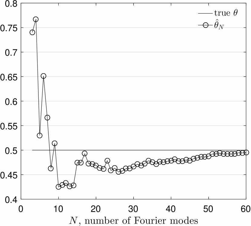
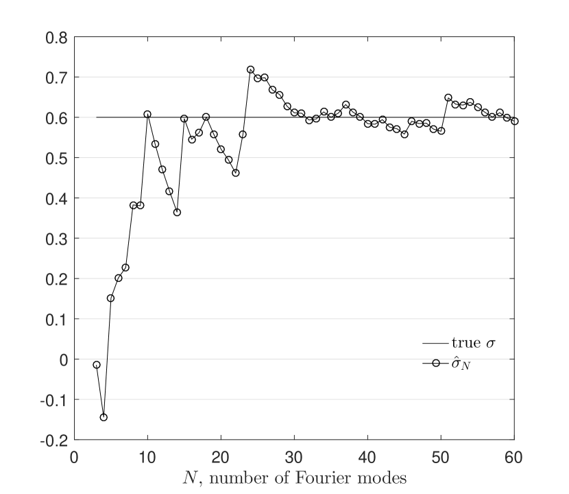
Figure 1. Shell model. Sample path of $\hat{\theta}_{N}$ (left panel) and $\hat{\sigma}_{N}$ (right panel).

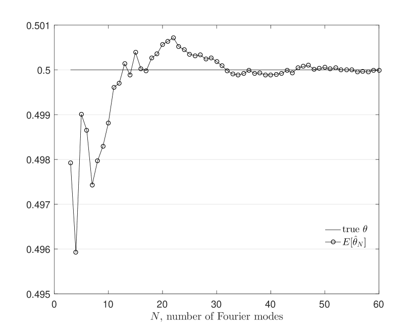
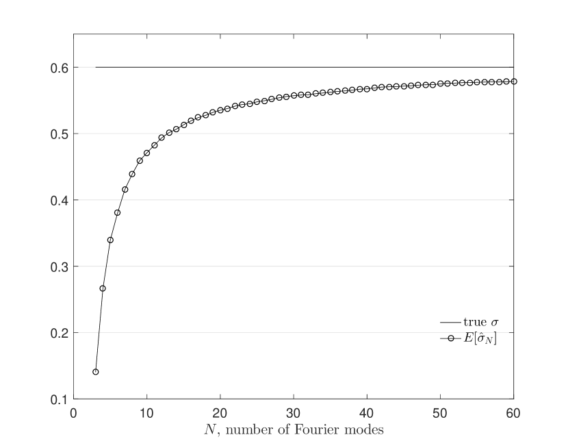
Figure 2. Shell model. Sample mean of $\hat{\theta}_{N}$ (left panel) and $\hat{\sigma}_{N}$ (right panel).

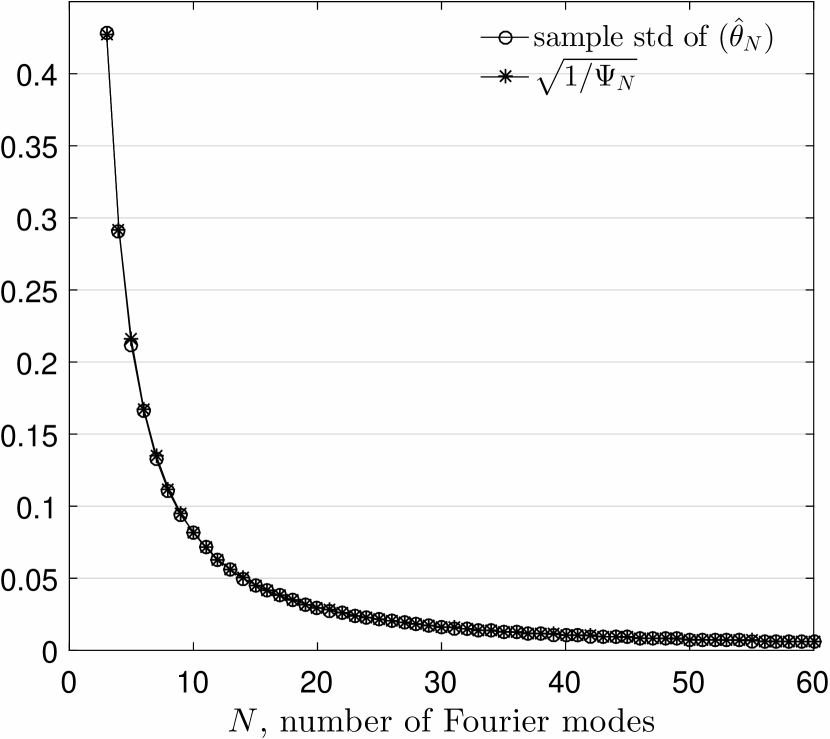
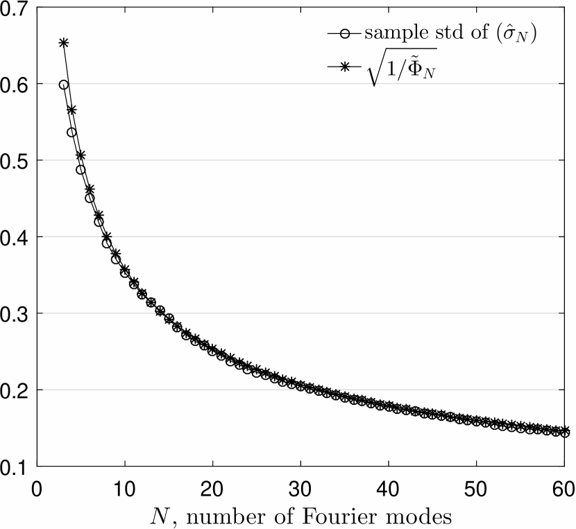
Figure 3. Shell model. Left panel: Sample standard deviation of $\hat{\theta}_{N}$ and theoretical standard deviation $\sqrt{1/\Psi_{N}}$ from asymptotic normality; Right panel: Sample standard deviation of $\hat{\sigma}_{N}$ and theoretical standard deviation $\sqrt{1/\widetilde{\Phi}_{N}}$, where $\widetilde{\Phi}_{N}$ is the Fisher information for $\hat{\sigma}_{N}$.

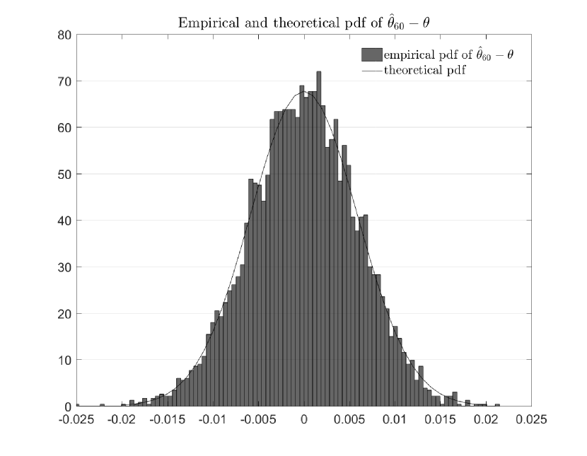
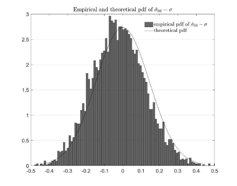
Figure 4. Shell model. Empirical distribution of $\hat{\theta}_{60}-\theta$ (left panel) and $\hat{\sigma}_{60}-\sigma$ and the pdf (solid lines) of the theoretical normal distribution from asymptotic normality.

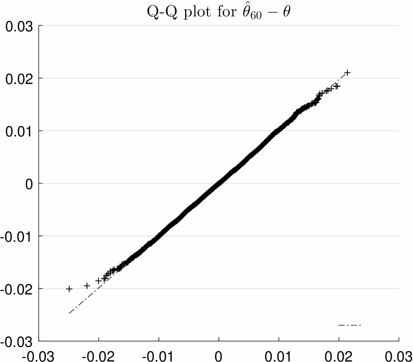
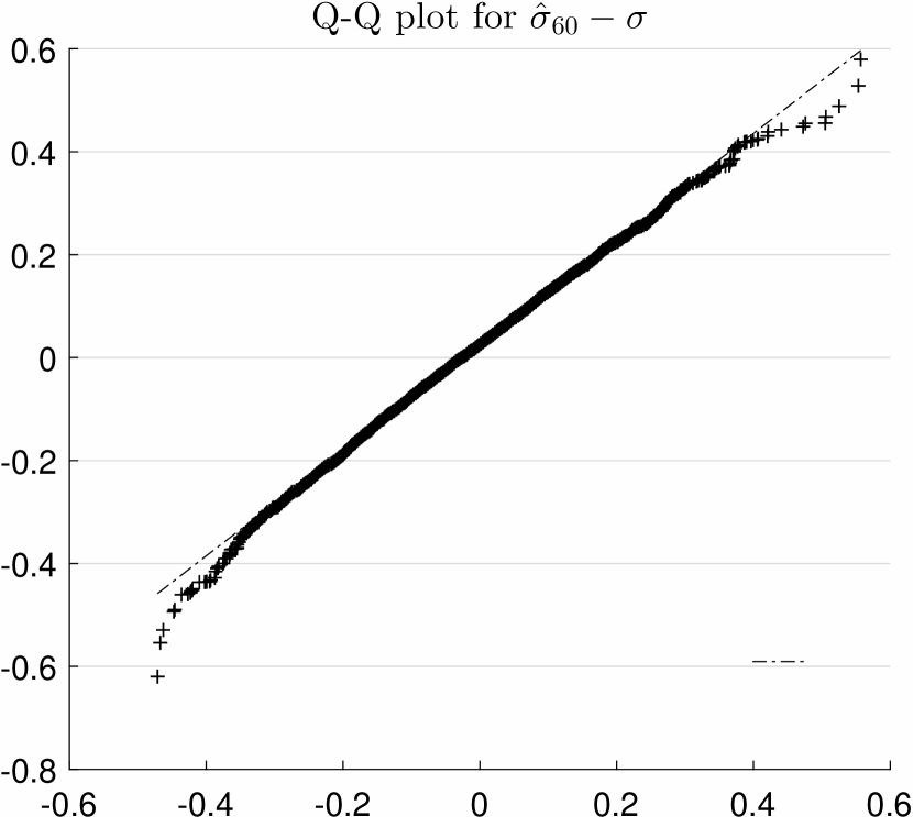
Figure 5. Shell model. Q-Q-Plot of $\hat{\theta}_{60}-\theta$ (left panel) and $\hat{\sigma}_{60}-\sigma$ vs the corresponding theoretical normal distribution from asymptotic normality.

Remark 5.1.

We ran the numerical experiments for different shell models of the type (4.1), and all obtained results agree with theoretical ones. For example, with $\mu_{k}=1,\ \nu_{k}=k^{4},\ q_{k}=k,\ p_{k}=0$ and all other parameters as in Example 2, the solution exists, but (2.19) is not satisfied, and as expected, estimators do not converge. On the other hand, with $\mu_{k}=k^{2},\ q_{k}=k^{3/2},\ \nu_{k}=p_{k}=0$, solution of (4.1) does not exists, but (2.19) and (2.20) are satisfied, and formally computed estimates converge. Other set of parameters, e.g. $\mu_{k}=k^{2},\ \nu_{k}=0,\ q_{k}=k^{\frac{1}{4}}(\log(1+k))^{\frac{1}{2}},\ p_{k}=0$, for which the solution exists and (2.19) and (2.20) are satisfied, produce similar results as in Example 1. We also computed the estimates for $\theta$ and $\sigma$ using Bayesian approach, and overall the results look similar to the MLE, although they are less stable numerically and more advanced numerical methods may need to be implemented.

Example 2. Additive noise. We consider the equation (4.5), with $\beta=1$, $G=[0,\pi]$, $d=1$. Thus, $\lambda_{k}=k^{2},\ h_{k}(x)=\sqrt{2/\pi}\sin(kx),\ k\in\mathbb{N}$, and we take the following set of parameters

$$\theta_{0}=0.1,\ \sigma_{0}=0.1,\ T=1,\ q_{k}=1,u(0)=0.$$

We will use similar numerical experiments as in Example 1, and compute the Fourier modes $u_{k}$ by applying directly (1.8). First we assume that $\sigma$ is known and apply Theorem 3.2 and, respectively, Theorem 3.3 to compute ‘the exact estimators’ for $\theta$ by using the values of the Fourier modes at two time points and, respectively, three time points, not counting the value at $t=0$. The obtained estimated value $\theta^{\prime}$ for $\theta$ are virtually indistinguishable from the true parameter, with the relative error $|\theta^{\prime}-\theta|/\theta<10^{-12}$, for any combination of chosen time points in $(0,1)$, and/or the Fourier mode $u_{k},k=1,\ldots,60$.

Next we assume that $\theta$ is known, and we estimate $\sigma$ by the MLE from Theorem 3.5. We conducted several numerical experiments to confirm the results of Theorem 3.5, and all experiments produced results similar to what we present below. In Figure 6 (left panel) we display one typical realization of $\hat{\sigma}_{N}$ (circled lines), which converges to the true value $\sigma=0.1$ (solid line). Using $5,\!000$ simulated paths of the first 55 Fourier coefficients, we compute the sample mean of $\hat{\sigma}_{N}$, presented in Figure 6 (right panel). Sample standard deviation of $\hat{\sigma}_{N}$ and its theoretical value from the asymptotic normality, are displayed in Figure 7 (left panel). Similar to Example 1, the sample mean of the estimates converges to the true value, as the number of the Fourier modes $N$ increases, and the sample standard deviation of the estimates converges to zero at the rate predicted by the asymptotic normality property. Finally, in Figure 7 (right panel), we present the empirical distribution of $\hat{\sigma}_{N}-\sigma$ for $N=55$, on which we superposed the distribution of Gaussian random variable (solid line) with mean zero and variance $\sigma^{2}/(2N)$, which validate the asymptotic normality of the estimators. Various other model parameterizations consistently yield similar results, and the obtained numerical results agree with the theoretical results on consistency and asymptotic normality of $\hat{\sigma}_{N}$ from Theorem 3.5.

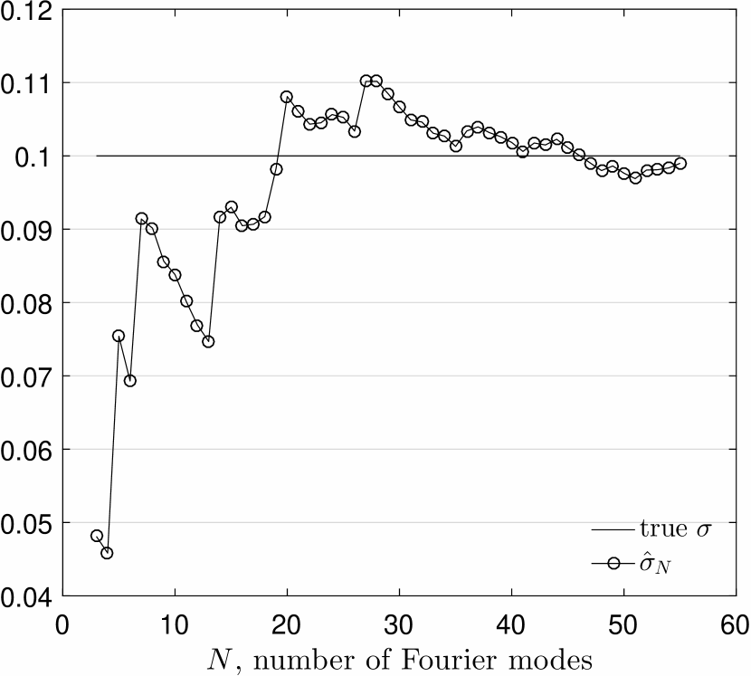
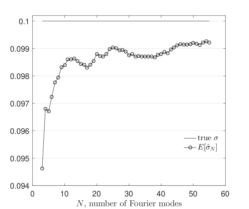
Figure 6. Additive noise. One sample path of $\hat{\sigma}_{N}$ (left panel) and the sample mean of $\hat{\sigma}_{N}$ (right panel).

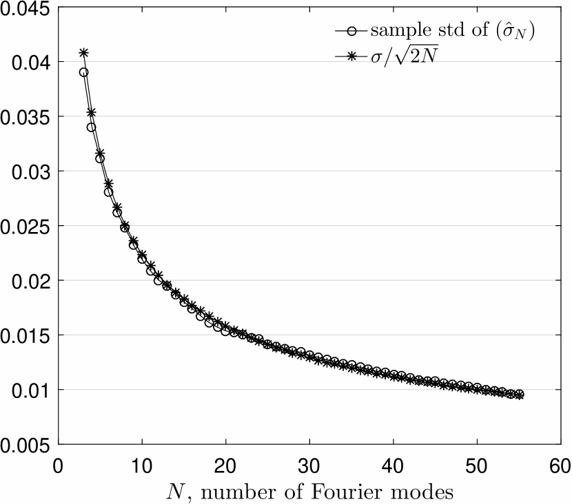
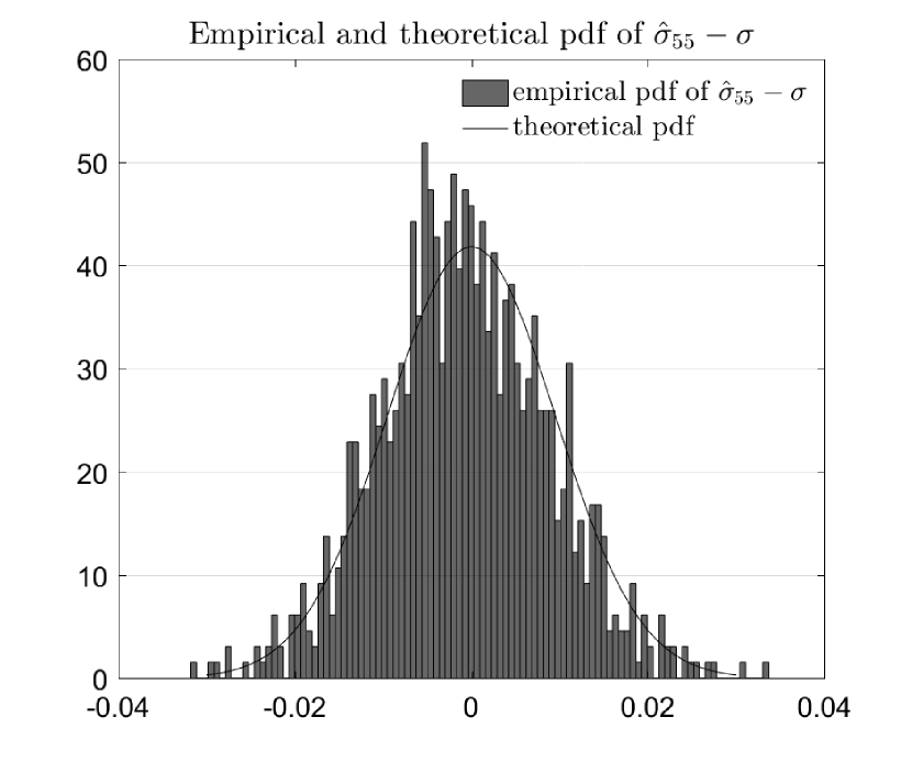
Figure 7. Additive noise. Sample standard deviation of $\hat{\sigma}_{N}$ and theoretical standard deviation $\sigma\sqrt{1/2N}$ from asymptotic normality (left panel) and empirical distribution of $\hat{\sigma}_{55}-\theta$ and the pdf (solid lines) of the theoretical normal distribution from asymptotic normality (right panel).

We conclude this example by applying the results from Section 3.2, assuming that $\sigma$ is known and $\theta$ is the parameter of interest. We postulate that the observer takes measurements of the spacial derivative of the solution $u_{x}$ at a fixed time point $t=0.2$ and over a space interval $[0,x]\subset[0,\pi]$. We approximate the function $u_{x}$ using the series representation (3.4), and by taking the first $30,\!000$ terms in the series and a space resolution of $0.0015$. In Figure 8 (left panel) we display the estimates $\check{\theta}_{M}$, and $\check{\sigma}_{M}$, given by (3.8), and (3.9), and using the values of $u_{x}(t,\cdot)$ from interval $[0,x]$, for a set of values of $x\in(0,\pi]$. The obtained values are close to the true values. We also applied a similar approach to study the estimators (3.10) and (3.11). However, the slow convergence rate of the Fourier series combined with low smoothness order of $u$ produce less desirable numerical results, see Figure 8 (right panel). Further investigations are needed, tentatively by employing more accurate numerical methods to approximate the solution.

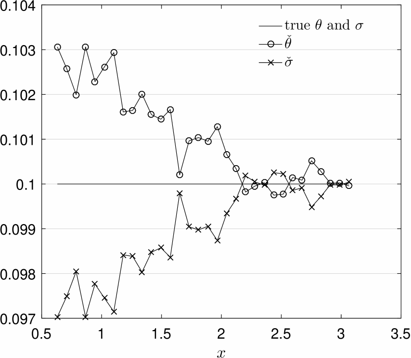
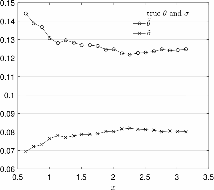
Figure 8. Additive noise. Discrete sampling. Left panel: values of $\check{\theta}$ and $\check{\sigma}$ by using values of $u_{x}(t,\cdot)$. Right panel: values of $\tilde{\theta}$ and $\tilde{\sigma}$ by using values of $u(t,\cdot)$. The horizontal axes $x$ indicates the right end point of $[0,x]$ over which the values of $u_{x}$ and $u$ were computed.

References

- [1] Z. Cheng, I. Cialenco, and R. Gong. Bayesian estimations for diagonalizable bilinear SPDEs. Forthcoming in Stochastic Process. Appl., 2019.
- [2] I. Cialenco and Y. Huang. A note on parameter estimation for discretely sampled SPDEs. Preprint arXiv:1710.01649, 2017.
- [3] I. Cialenco. Statistical inference for SPDEs: an overview. Statistical Inference for Stochastic Processes, 21(2):309–329, 2018.
- [4] I. Cialenco and S. V. Lototsky. Parameter estimation in diagonalizable bilinear stochastic parabolic equations. Stat. Inference Stoch. Process., 12(3):203–219, 2009.
- [5] S. Friedlander, N. Glatt-Holtz, and V. Vicol. Inviscid limits for a stochastically forced shell model of turbulent flow. Ann. Inst. Henri Poincaré Probab. Stat., 52(3):1217–1247, 2016.
- [6] U. Frisch. Turbulence. Cambridge University Press, Cambridge, 1995.
- [7] N. Glatt-Holtz and M. Ziane. The stochastic primitive equations in two space dimensions with multiplicative noise. Discrete Contin. Dyn. Syst. Ser. B, 10(4):801–822, 2008.
- [8] M. Huebner and B. L. Rozovskii. On asymptotic properties of maximum likelihood estimators for parabolic stochastic PDE’s. Probab. Theory Related Fields, 103(2):143–163, 1995.
- [9] I. A. Ibragimov and R. Z. Has’minskiĭ. Statistical estimation: Asymptotic theory, volume 16 of Applications of Mathematics. Springer-Verlag, New York-Berlin, 1981.
- [10] S. Kakutani. On equivalence of infinite product measures. Ann. of Math. (2), 49:214–224, 1948.
- [11] H.-J. Kim and S. V. Lototsky. Time-homogeneous parabolic Wick-Anderson model in one space dimension: regularity of solution. Stoch. Partial Differ. Equ. Anal. Comput., 5(4):559–591, 2017.
- [12] F. C. Klebaner. Introduction to stochastic calculus with applications. Imperial College Press, London, second edition, 2005.
- [13] S. V. Lototsky and B. L. Rozovsky. Stochastic partial differential equations. Universitext. Springer International Publishing, 2017.
- [14] S. V. Lototsky and B. L. Rozovsky. Stochastic Evolution Systems. Linear theory and applications to non-linear filtering, volume 89 of Probability Theory and Stochastic Modelling. Springer International Publishing, second edition, 2018.
- [15] I. Nourdin, G. Peccati, and Y. Swan. Entropy and the fourth moment phenomenon. J. Funct. Anal., 266(5):3170–3207, 2014.
- [16] A. N. Shiryaev. Probability, volume 95 of Graduate Texts in Mathematics. Springer-Verlag, New York, second edition, 1996.
- [17] M. A. Shubin. Pseudodifferential operators and spectral theory. Springer-Verlag, Berlin, second edition, 2001.