Noise-Level Estimation from Single Color Image
Using Correlations Between Textures in RGB Channels

Abstract

We propose a simple method for estimating noise level from a single color image. In most image-denoising algorithms, an accurate noise-level estimate results in good denoising performance; however, it is difficult to estimate noise level from a single image because it is an ill-posed problem. We tackle this problem by using prior knowledge that textures are highly correlated between RGB channels and noise is uncorrelated to other signals. We also extended our method for RAW images because they are available in almost all digital cameras and often used in practical situations. Experiments show the high noise-estimation performance of our method in synthetic noisy images. We also applied our method to natural images including RAW images and achieved better noise-estimation performance than conventional methods.

1 Introduction

Noise-level estimation is an important research area in computer vision and has many applications such as image denoising [3, 7, 14, 23] and edge detection [8]. It is important for these applications to obtain a good noise-level estimate in advance because their performance strongly depends on the accuracy of this estimate. However, noise-level estimation from a single image is fundamentally an ill-posed problem, and it is impossible to separate noise from textures in a single image without using prior knowledge. To tackle this problem, many methods have been developed, such as PCA-based and learning-based ones, but most do not exploit the relationship between channels in color images.

We focus on the high correlations between channels in color images and propose a noise-level estimation method using an assumption that textures are highly correlated between RGB channels and noise is uncorrelated with other signals (Figure 1). We also extended our method for RAW images because they are often used in practical situations and available in almost every digital camera. We applied the proposed method to images artificially degraded with Gaussian noise and succeeded in accurately estimating the noise level. We also applied our method to natural noisy images including RAW images, and it achieved better noise-estimation performance than conventional methods.

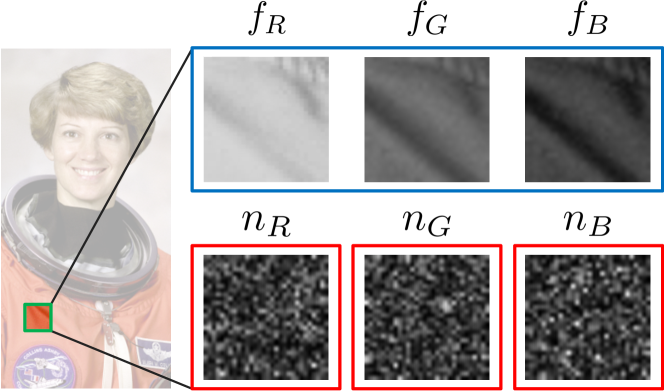
Figure 1: Left: With proposed method, small patches are sampled from input image. Right: Observed image is composed of noise-free image $f_{c}$ and noise $n_{c}\ (c\in\{R,G,B\})$. We assume that noise-free image $f_{c}$ is correlated between RGB channels and noise $n_{c}$ is uncorrelated with other signals.

The main contribution of this paper is:

• We propose a method of estimating noise level in a single color image using an assumption that noise-free pixel values are often correlated between RGB channels while noise is uncorrelated. We believe we are the first to propose a channel-correlation-based method.

2 Related Work

Noise-level estimation from a single image is an ill-posed problem because it is impossible to completely separate textures from noise, and many methods have been developed to tackle this problem [9, 10, 15, 25]. Some methods succeeded in estimating noise level by using patches sampled from homogeneous areas [2, 20, 21, 22]. These methods are based on the assumption that there is a sufficient amount of flat areas in the input image, but this assumption does not necessarily hold in natural images with rich textures. Another method approximates noise by taking the difference between the original image and blurred image [18]. However, the noise level is often overestimated with these methods because high-frequency components of textures still remain in the difference image. PCA-based methods have been proposed [16, 19] to avoid these problems. The core idea of PCA-based methods is that textures lie in a low-dimensional subspace and the noise level can be estimated using eigenvalues of the redundant dimensions. However, Chen et al. [5] pointed out that the noise level is underestimated with these methods. They further investigated this problem and succeeded in improving the performance of PCA-based methods by statistically analyzing the eigenvalues of the redundant space [5]. The PCA-based methods discussed above work well when the image is degraded with white noise but fail to estimate noise level accurately if the image contains non-white noise. This is because non-white noise does not distribute uniformly in the redundant dimensions.

A fast patch-based noise-estimation method has recently been proposed [11] using the Canny edge detector [4] to exclude highly textured areas. This method is fast because of its simplicity, but the parameters of the edge detector have to be properly set to correctly detect areas with rich textures. Learning-based noise-estimation methods [24] and denoising methods [6, 26] using convolutional neural networks [13] have also been proposed recently. These methods achieve high performance in noise estimation and denoising but suffer from high computational costs of convolutions for real-time computing when sufficient computational resources are not available such as in smartphones.

We propose a noise-level-estimation method using an assumption that textures are highly correlated between RGB channels while noise is uncorrelated with other signals. The proposed method does not require flat areas in the input image, the assumption that the input image contains white noise, sophisticated parameter tuning, and a significant amount of computational resources.

3 Noise Estimation with RGB Correlations

3.1 Assumptions

A model for a noisy RGB image with additive noise is given by

$$I_{c}=f_{c}+n_{c}\ \ \ \left(c\in\{R,G,B\}\right)$$ (1)

where $I_{c}$ is the observed noisy image, $f_{c}$ is the noise-free image (texture), and $n_{c}$ is noise. We assume that textures are correlated between RGB channels and noise is uncorrelated with other signals in image patch $P_{i}$. This is expressed as

$$\underset{P_{i}}{\mathrm{Cov}}\,\left[f_{c},f_{c^{\prime}}\right] =S_{\mathit{cc^{\prime}}}$$ (2)

$$\underset{n}{\mathrm{E}\,}\left[\underset{P_{i}}{\mathrm{Cov}}\,\left[f_{c},n_{c^{\prime}}\right]\right] =0$$ (3)

$$\underset{n}{\mathrm{E}\,}\left[\underset{P_{i}}{\mathrm{Cov}}\,\left[n_{c},n_{c^{\prime}}\right]\right] =0\ \ \ (c\neq c^{\prime})$$ (4)

for $c,c^{\prime}\in\{R,G,B\}$, where $\underset{P_{i}}{\mathrm{Cov}}\,[\cdot,\cdot]$ is the covariance operator in patch $P_{i}$, $S_{\mathit{cc^{\prime}}}$ is the covariance between noise-free images in each channel, and $\underset{n}{\mathrm{E}\,}[\cdot]$ is the expected value with respect to noise $n$. We also assume that each channel has the same noise level:

$$\underset{n}{\mathrm{E}\,}\left[\underset{P_{i}}{\mathrm{Var}}\,\left[n_{c}\right]\right]=\sigma^{2}\ \ \ (c\in\{R,G,B\})$$ (5)

Here, $\underset{P_{i}}{\mathrm{Var}}\,[\cdot]$ is the variance operator in patch $P_{i}$, and $\sigma$ is the ground-truth noise level.

3.2 Proposed Method

3.2.1 Noise-Level Estimation

Let $\alpha_{i}$ and $\beta_{i}$ be the variables obtained from randomly sampled image patch $P_{i}\,(i=1,2,\ldots,N_{p})$ by calculating

$$\alpha_{i} =\frac{\underset{P_{i}}{\mathrm{Var}}\,[I_{R}]+\underset{P_{i}}{\mathrm{Var}}\,[I_{G}]+\underset{P_{i}}{\mathrm{Var}}\,[I_{B}]}{3}$$ (6)

$$\beta_{i} =\underset{P_{i}}{\mathrm{Var}}\,\left[\frac{I_{R}+I_{G}+I_{B}}{3}\right]$$ (7)

In other words, variable $\alpha_{i}$ is the mean of the channelwise-variance of pixel values (mean of variance) and variable $\beta_{i}$ is the variance of pixel values in the mean image (variance of mean). The following equation and inequality hold for $\alpha_{i}$ and $\beta_{i}$:

$$\underset{n}{\mathrm{E}\,}\left[\alpha_{i}\right] =\frac{S_{R}^{2}+S_{G}^{2}+S_{B}^{2}}{3}+\sigma^{2}$$ (8)

$$\underset{n}{\mathrm{E}\,}\left[\beta_{i}\right] \leq\frac{S_{R}^{2}+S_{G}^{2}+S_{B}^{2}}{3}+\frac{1}{3}\sigma^{2}$$ (9)

where $S_{c}^{2}\ (c\in\{R,G,B\})$ is the variance of the noise-free image $f_{c}$ in patch $P_{i}$ (details are shown in the appendix). Both sides of Inequality 9 are equal if condition $C$ is satisfied:

$$C f_{c}-f_{c^{\prime}}\ (c\neq c^{\prime})\ \ P_{i}$$: is constant in each channel of patch (10)

In other words, condition $C$ is equivalent to the following condition: pixel values of a difference image between two channels are constant in patch $P_{i}$. By substituting Equation 8 into Inequality 9, we have

$$\sigma^{2}\leq\underset{n}{\mathrm{E}\,}\left[\frac{3}{2}(\alpha_{i}-\beta_{i})\right]$$ (11)

with equality if condition $C$ is satisfied.

Inequality 11 shows that the right side is a good approximation of the ground-truth noise level if condition $C$ is satisfied. Therefore, noise-level estimate $\tilde{\sigma}_{i}^{2}$ for each patch $P_{i}$ is given by

$$\tilde{\sigma}_{i}^{2}=\frac{3}{2}(\alpha_{i}-\beta_{i})$$ (12)

Now, we have the noise-level estimate of the entire image $\tilde{\sigma}^{2}$ as the weighted mean of $\tilde{\sigma}_{i}^{2}$:

$$\tilde{\sigma}^{2}=\left(\sum_{i=1}^{N_{p}}w_{i}\tilde{\sigma}_{i}^{2}\right)\Bigg{/}\left(\sum_{i=1}^{N_{p}}w_{i}\right)$$ (13)

where $w_{i}$ is a weight whose value depends on to what extent condition $C$ is satisfied, and $N_{p}$ is the number of sampled patches. The details of weight determination are explained in the next section.

3.2.2 Weight Determination

The accuracy of noise-level estimate $\tilde{\sigma}_{i}^{2}$ depends on to what extent condition $C$ is satisfied, so we define loss $L_{i}$ for each patch as

$$L_{i}=\frac{\underset{P_{i}}{\mathrm{Var}}\,[f_{R}-f_{G}]+\underset{P_{i}}{\mathrm{Var}}\,[f_{G}-f_{B}]+\underset{P_{i}}{\mathrm{Var}}\,[f_{B}-f_{R}]}{3}$$ (14)

However, the exact value of loss $L_{i}$ cannot be obtained since noise-free image $f_{c}\,(c\in\{R,G,B\})$ is unknown. Therefore, we approximate loss $L_{i}$ by

$$\tilde{L}_{i}=\frac{\underset{P_{i}}{\mathrm{Var}}\,[I^{\prime}_{R}-I^{\prime}_{G}]+\underset{P_{i}}{\mathrm{Var}}\,[I^{\prime}_{G}-I^{\prime}_{B}]+\underset{P_{i}}{\mathrm{Var}}\,[I^{\prime}_{B}-I^{\prime}_{R}]}{3}$$ (15)

where $I^{\prime}_{c}$ is an image blurred with a Gaussian filter with the standard deviation of $\sigma_{\mathrm{blur}}$. This results in better noise-estimation performance than simply using the original image $I_{c}$ because blurred image $I^{\prime}_{c}$ approximates noise-free image $f_{c}$ by removing the noise from original image $I_{c}$. Note that the blurring does not affect the correlations between RGB channels since the filter is independently applied to each channel with the same blur strength.

Weight $w_{i}$ should be large when the loss is small and vice versa, so we define weight $w_{i}$ as

$$w_{i}=\exp\left(-\gamma\frac{\tilde{L}_{i}}{\sum_{j=1}^{N_{p}}\tilde{L}_{j}/N_{p}}\right)$$ (16)

where $\sum_{j}\tilde{L}_{j}/N_{p}$ is the normalization factor of $\tilde{L}_{i}$, and $\gamma$ is a parameter that determines how strongly patches with high losses are filtered out (we also manually exclude patches if they contain an overexposed or underexposed area because noise levels in such areas are considered smaller than the true noise level). In Section 4.1.2, we experimentally show how parameter $\gamma$ affects noise-estimation performance.

3.3 Extension for RAW Images

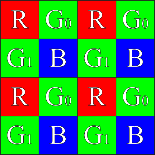
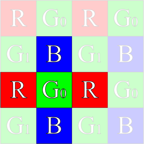
Figure 2: Left: Bayer pattern of RAW image. Green cells are divided into two subgroups $G_{0}$ and $G_{1}$, so numbers of cells $R$, $G_{0}$, $G_{1}$ and $B$ are same. Right: We calculate red and blue components at each cell $G_{0}$ by taking average of neighbor cells. In same way, red and blue components are calculated at each cell $G_{1}$.

In this section, we discuss extending our method for RAW images. A RAW image contains unprocessed sensor outputs in the Bayer pattern, as shown in Figure 2. Note that the green cells are divided into two subgroups $G_{0}$ and $G_{1}$ so that each group ($R$, $G_{0}$, $G_{1}$, and $B$) has the same number of cells. We interpolate the red and blue components at each green cell by averaging neighbor cells, as shown in Figure 2.

Now, we obtain two sub-images $I^{(0)}$ and $I^{(1)}$ by extracting the RGB components from subgroups $G_{0}$ and $G_{1}$, respectively. Note that these sub-images are half the size of the original RAW image since the sampling is carried out with the stride of two. By concatenating patches $P_{i}^{(0)}$ and $P_{i}^{(1)}$ sampled in the same area from sub-images $I^{(0)}$ and $I^{(1)}$, we obtain patch $P_{i}$, which can be treated in the same manner as that discussed in Section 3.2.1. Note that the noise variance of the red and blue components in the sub-images is $\sigma^{2}/2$ since they are obtained by averaging two pixels of the original RAW image. Therefore, Equation 8 and Inequality 9 should be as follows:

$$\underset{n}{\mathrm{E}\,}\left[\alpha_{i}\right] =\frac{S_{R}^{2}+S_{G}^{2}+S_{B}^{2}}{3}+\frac{2}{3}\sigma^{2}$$ (17)

$$\underset{n}{\mathrm{E}\,}\left[\beta_{i}\right] \leq\frac{S_{R}^{2}+S_{G}^{2}+S_{B}^{2}}{3}+\frac{2}{9}\sigma^{2}$$ (18)

By substituting Equation 17 into Inequality 18, the noise-level estimate of each patch for RAW images is given as

$$\tilde{\sigma}_{i}^{2}=\frac{9}{4}(\alpha_{i}-\beta_{i})$$ (19)

4 Experiments

In this section, we first discuss noise-estimation performance of the proposed method for images artificially degraded with Gaussian noise. Next, we analyze the relationship between parameter $\gamma$ and patch size, which are both import parameters in the proposed method, to show that the noise-estimation performance of our method increases by using the weighted mean of the noise estimates rather than using the unweighted mean in Equation 13. Then we evaluate the noise-estimation performance of our method for natural noisy images and analyze the noise correlations in these images, which affects the noise-estimation performance of our method. Finally, we compare the noise-estimation performance of our method to those of conventional methods.

In our experiments, we used JPEG and RAW images taken with a digital camera (Sony ILCD-7S). We also generated lossless PNG images from the RAW images using ImageMagick [1] to exclude the effects of JPEG compression. For simplicity, we normalized the images by dividing them by 255 so that all pixel values are within the range of $[0,1]$.

4.1 Evaluation

4.1.1 Artificially Degraded Images

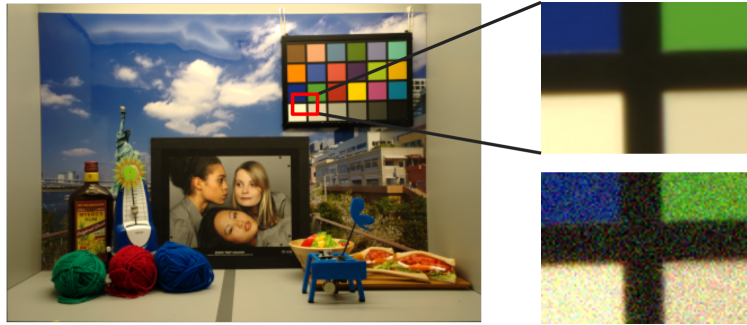
Figure 3: Left: Noise-free image obtained by taking average of 10 clear images. Upper right: Close-up of noise-free image. Lower right: Close-up of synthetic noisy image with Gaussian noise (ground-truth noise level: $\sigma=0.095$).

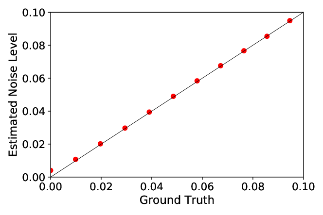
Figure 4: Relation between synthetic Gaussian-noise level and noise estimates with proposed method. Line $y=x$ in this figure shows ideal noise-estimation result.

We evaluated the noise-estimation performance of our method for synthetic noisy images generated by adding Gaussian noise to a noise-free image (Figure 3). The noise-free image was generated by taking the average of 10 static images taken under good photographic conditions (ISO: 50, exposure time: $2.5\,\mathrm{s}$). We then added the Gaussian noise to the noise-free image and truncated the pixel values so that they stay in the range of $[0,1]$. We applied the proposed method to the synthetic noisy images and compared the noise estimates with the ground-truth noise levels. The ground-truth noise level was obtained in the following manner: first, we generated ten noisy images by adding Gaussian noise of the same noise level to the noise-free image; second, we calculated the pixel value variances across the ten images at each pixel; finally, we obtained the ground-truth noise level by taking the squared root of the mean of variances calculated in the second step. Note that the ground-truth noise level is slightly smaller than the standard deviation of the Gaussian noise since the pixel values are truncated to stay in the range of $[0,1]$. The parameters were set as follows: $\gamma=2.0$, $k=5$, $N_{p}=1000$, and $\sigma_{\mathrm{blur}}=5.0$ where $\gamma$ is a parameter that determines how strongly patches with high losses are filtered out, $k$ is the patch size, $N_{p}$ is the number of sampled patches, and $\sigma_{\mathrm{blur}}$ is the standard deviation of Gaussian filter used in weight determination.

Figure 4 shows that our method succeeded in accurately estimating the ground-truth noise level. However, it slightly overestimated the noise level when the ground-truth noise level was very small ($\sigma\leq 0.01$). This is considered to be the noise that could not be completely eliminated in the noise-free image.

4.1.2 Relation Between Parameter $\gamma$ and Patch Size

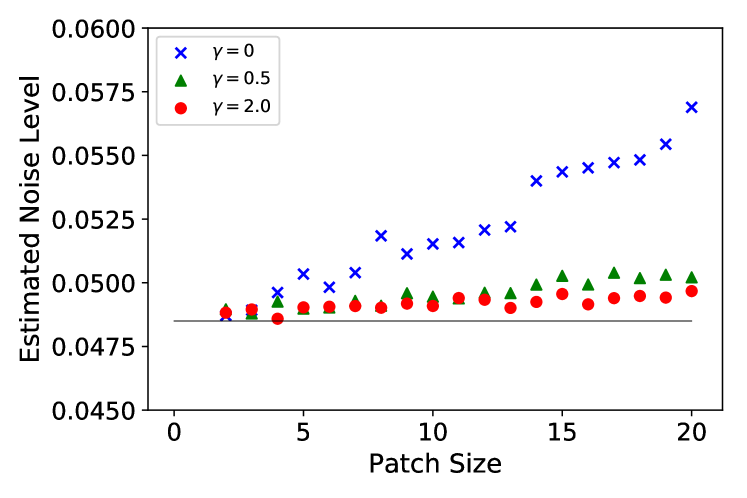
Figure 5: Relation between patch size and noise estimates with different parameter $\gamma$ values. When parameter $\gamma$ is large enough, noise estimate is almost independent of patch size and closer to ground-truth noise level ($\sigma=0.0485$).

In this section, we show that the noise estimate is independent of patch size if we use the weighted mean of the noise estimates (Equation 13), while the noise estimate is affected by patch size if we simply take the unweighted mean. We analyzed the relation between the accuracy of noise estimates and patch size while changing parameter $\gamma$. The ground-truth noise level ($\sigma=0.0485$) was calculated in the same manner as that discussed in Section 4.1.1. We set the parameters as follows: $\gamma\in\{0,0.5,2.0\}$, $k\in\{2,3,4,\ldots,20\}$, $N_{p}=1000$, and $\sigma_{\mathrm{blur}}=5.0$. As mentioned above, parameter $\gamma$ determines how strongly patches with high losses are filtered out, so Equation 13 is equivalent to taking the unweighted mean when parameter $\gamma$ is set to zero.

Figure 5 shows that the noise estimate is closer to the ground truth and independent of the patch size when parameter $\gamma$ is large enough. This means that the noise-estimation performance of our method improved using the weighted mean rather than unweighted mean. Interestingly, the noise estimate increases as the patch size increases if we use the unweighted mean (i.e. $\gamma=0$). This can be explained as follows. If the patch size is large, we are more likely to have patches that do not satisfy condition $C$, and this results in a larger expectation value of noise estimates, as shown in Inequality 11. We avoid this problem by using the weighted mean to exclude these patches. Note that parameter $\gamma$ should not be too large because there is a lack of noise-estimate samples from filtering out most of the noise estimates.

4.1.3 Natural Images

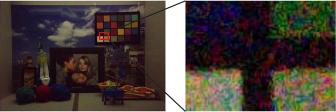
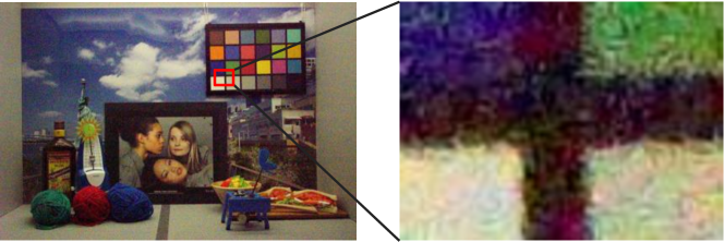
Figure 6: Sample natural noisy images used in experiments. Upper: Noisy PNG image and close-up. Lower: Noisy JPEG image and close-up.

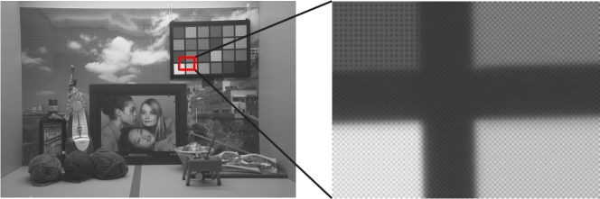
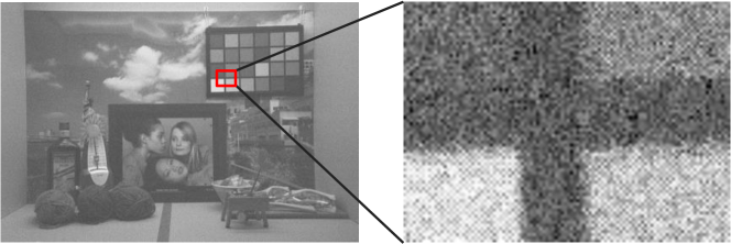
Figure 7: RAW images used in experiments. Note that RAW image can be visualized as gray-scale image. Upper: Clean RAW image and close-up. Bayer pattern can be observed, which is unique to RAW images. Lower: Noisy RAW image and close-up. Image is strongly degraded but Bayer pattern still can be observed (recommended to view this figure in electronic version to obtain clear view of Bayer pattern).

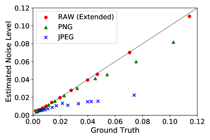
Figure 8: Results of noise estimation for natural images. Our extended method was applied to RAW images and original method was applied to PNG and JPEG images.

We evaluated the noise-estimation performance of our method for natural noisy images (Figures 6 and 7). In this experiment, we used RAW, PNG, and JPEG images with various noise levels under different photographic conditions ([ISO, exposure time] = [50, $1\,\mathrm{s}$] to [409600, $1/8000\,\mathrm{s}$]). The RAW and JPEG images were directly obtained from the camera, and the PNG images were generated from the RAW images. We calculated the ground-truth noise level in the same manner as that discussed in Section 4.1.1 using 20 static images taken under the same photographic conditions. The parameters were set as follows: $\gamma=2.0$, $k=5$, $N_{p}=1000$, and $\sigma_{\mathrm{blur}}=5.0$.

Figure 8 shows that our method estimated noise levels very accurately for the natural noisy RAW images in a wide range of noise levels [0.0, 0.12]. However, the noise-estimation performance for the PNG and JPEG images was lower than for the RAW images. This is because of the noise correlations between RGB channels in natural noisy images. We have so far assumed that noise is uncorrelated between RGB channels; however, it has been shown that this assumption does not necessarily hold in natural images because RGB channels are mixed up during in-camera processing and JPEG compressions [12, 17]. Note that our focus here is on the effect of JPEG compression on image noise, rather than the noise called JPEG artifacts or mosquito noise. Nam et al. [17] showed that in-camera processing and JPEG compression affect the noise characteristics, and the noise correlations caused by these processes cannot be ignored. They also showed that the noise in each channel is almost uncorrelated in RAW images (we analyze the noise correlations in natural images in Section 4.2). Therefore, the noise correlation is considered to be the main cause of the decrease in noise-estimate performance for natural PNG and JPEG images. Although the noise-estimation performance of our method decreased in these images, it is much better than those of the conventional methods, which are discussed in Section 4.3.2.

4.2 Noise Correlations Between RGB Channels

Table 1: Noise correlation coefficients in natural images of different formats. RAW (0) and RAW (1) correspond to $I^{(0)}$ and $I^{(1)}$ in Section 3.3, respectively.

	$r_{RG}\ \$	$r_{GB}\ \$	$r_{GB}\ \$
RAW (0)	0.0031	0.0011	0.0025
RAW (1)	-0.0002	0.0041	0.0025
PNG	-0.0855	-0.1414	-0.0572
JPEG	0.4852	0.5382	0.4755

We analyzed the noise correlations in natural images. We obtained a noise-free image by taking the average of 20 noisy static images (ISO: 409600, exposure time: $1/8000\,\mathrm{s}$) and calculated the noise by subtracting the noise-free image from the original noisy image. For RAW images, we used two sub-images $I^{(0)}$ and $I^{(1)}$ introduced in Section 3.3 since RGB channels were not available in the original RAW images. We calculated the noise correlations between RGB channels, as shown in Table 1. This shows that the noise correlations were high in the JPEG image ($|r|\approx 0.5$) while the RAW image had lower noise correlations ($|r|\approx 0.002$). The PNG image had higher noise correlations than the RAW image ($|r|\approx 0.09$), but was smaller than those of the JPEG image. The cause of the high noise correlations in the JPEG and PNG images is considered to be the developing processes and JPEG compression, as Nam et al. [17] pointed out.

4.3 Comparative Evaluation

We compared the noise-estimation performance of the proposed method to those of conventional PCA-based methods proposed by Chen et al. [5] and Liu et al. [16]. We conducted two experiments for this comparison. First, we compared the noise-estimation performance in synthetic noisy images degraded with Gaussian noise. Next, we used natural noisy RAW, PNG, and JPEG images to compare its noise-estimation performance for practical use.

4.3.1 Artificially Degraded Images

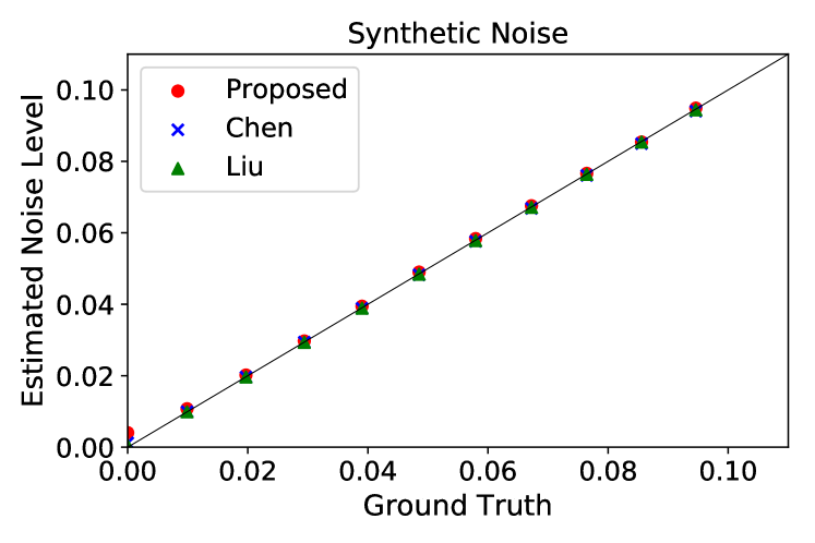
Figure 9: Comparison of noise-estimation performance for artificially degraded images. All methods achieved high noise-level-estimation performance.

In the same manner as that discussed in Section 4.1.1, we evaluated the noise-estimation performance of our method for synthetic noisy images. Figure 9 shows that all methods succeeded in estimating the noise level very accurately. Although the proposed method slightly overestimated the noise level compared to the conventional methods, the estimation error was very small and can be ignored for practical use (e.g. when the ground-truth noise level $\sigma$ was 0.04852, the estimation error was 0.00047, -0.00028, and -0.00010 with the proposed method, Chen et al.’s [5] and Liu et al.’s [16], respectively.)

4.3.2 Natural Images

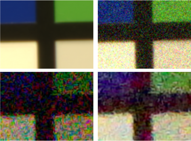
Figure 10: Close-up of images with same magnification ratio to compare noise patterns in detail. Upper left: Noise-free image. Upper right: Synthetic noisy image degraded with Gaussian white noise. Lower: Noisy PNG image (left) and noisy JPEG image (right). Recognizable spatial noise patterns can be observed in natural noisy images. This means that noise has spatial correlation in these images (recommended to view this figure in electronic version to obtain clear view of noise distribution).

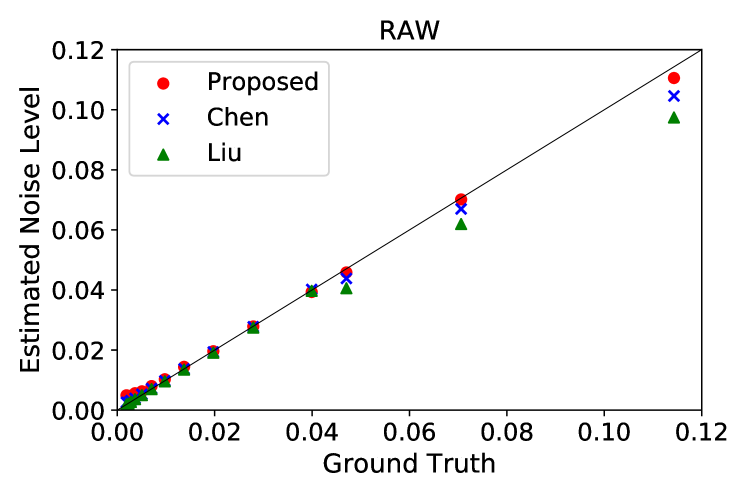
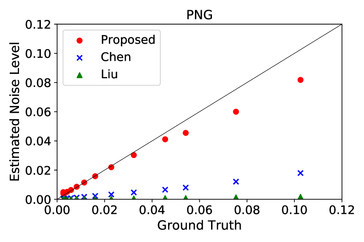
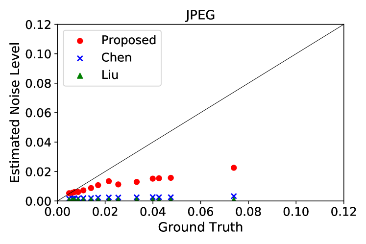
Figure 11: Comparison of noise-estimation performance in natural noisy images. Upper: Results from RAW images. Proposed method outperformed other methods, especially when ground-truth noise level was larger than 0.04. Middle: Results from PNG images. Proposed method better approximated ground-truth noise level while conventional methods failed. Lower: Results from JPEG images. All methods failed to estimate noise level, but noise estimates with proposed method were closer to ground truth compared to those of conventional methods.

We compared the noise-estimation performance using natural noisy RAW, PNG, and JPEG images in the same manner as that discussed in Section 4.1.3. The conventional methods cannot be directly applied to RAW images. Therefore, we generated four gray-scale images by extracting pixel values from each subgroup ($R$, $G_{0}$, $G_{1}$, and $B$) of the original RAW image, and calculated the noise estimate by averaging the noise estimates obtained from the gray-scale images. The results are shown in Figure 11. Although our method tended to overestimate the noise level when the ground-truth noise level was very small ($\sigma\leq 0.005$), it achieved higher accuracy than the conventional methods in every image format, which shows that our method is more suitable for practical use than conventional noise-estimation methods. Interestingly, the conventional methods failed to estimate the noise level in the natural PNG and JPEG images. These methods are based on the idea that the input image degrades with white noise. However, natural noise has spatial correlations, as shown in Figure 10, so it cannot be regarded as white noise; hence, the low noise-estimation performance of the conventional methods. On the other hand, the proposed method works well even if the input image is degraded with spatially correlated noise since our method is based on the assumption that noise is uncorrelated in the channel direction rather than in the spatial direction.

5 Conclusion

We proposed a simple method of estimating noise level from a single color image with prior knowledge that textures are correlated between RGB channels while noise is uncorrelated with other signals. We also extended our method for RAW images because they are useful and available in almost every digital camera. We experimentally discussed the noise-estimation performance of the proposed method for images degraded by synthetic Gaussian noise. We also applied the proposed method to natural RAW, PNG, and JPEG images, and it achieved higher noise-estimation performance than conventional noise-estimation methods.

Future work includes statistically analyzing the relationship between loss $\tilde{L}_{i}$ and noise estimates $\tilde{\sigma}_{i}$. Weight $w_{i}$ is heuristically determined in the proposed method, and it is not theoretically guaranteed that good patches are effectively selected with this weight. Therefore, noise-estimation performance of our method can be further improved by statistically analyzing these variables.

Appendix:
Detailed Explanation of Section 3.2.1

Let us define color channel set $U$ as $\{R,G,B\}$. Variable $\alpha_{i}$ defined in Section 3.2.1 is deformed as follows:

$$\alpha_{i} =\frac{1}{3}\sum_{c\in U}\underset{P_{i}}{\mathrm{Var}}\,[I_{c}]$$ (20)

$$=\frac{1}{3}\sum_{c\in U}\underset{P_{i}}{\mathrm{Var}}\,[f_{c}+n_{c}]$$ (21)

$$=\frac{1}{3}\sum_{c\in U}\left(\underset{P_{i}}{\mathrm{Var}}\,[f_{c}]+\underset{P_{i}}{\mathrm{Var}}\,[n_{c}]+2\,\underset{P_{i}}{\mathrm{Cov}}\,[f_{c},n_{c}]\right)$$ (22)

By using the assumptions in Section 3.1, the following formula is obtained:

$$\underset{n}{\mathrm{E}\,}\left[\alpha_{i}\right] =\frac{1}{3}\sum_{c\in U}\left(S_{c}^{2}+\sigma^{2}+0\right)$$ (23)

$$=\frac{1}{3}\left(S_{R}^{2}+S_{G}^{2}+S_{B}^{2}\right)+\sigma^{2}$$ (24)

In the same manner, variable $\beta_{i}$ is deformed as follows:

$$\beta_{i} =\underset{P_{i}}{\mathrm{Var}}\,\left[\frac{1}{3}\sum_{c\in U}I_{c}\right]$$ (25)

$$=\frac{1}{9}\ \underset{P_{i}}{\mathrm{Var}}\,\left[\sum_{c\in U}(f_{c}+n_{c})\right]$$ (26)

$$=\frac{1}{9}\ \sum_{c\in U}\left(\underset{P_{i}}{\mathrm{Var}}\,\left[f_{c}\right]+\underset{P_{i}}{\mathrm{Var}}\,\left[n_{c}\right]\right)$$

$$+\frac{1}{9}\sum_{c,c^{\prime}\in U\atop c\neq c^{\prime}}\left(\underset{P_{i}}{\mathrm{Cov}}\,\!\left[f_{c},f_{c^{\prime}}\right]+\underset{P_{i}}{\mathrm{Cov}}\,\!\left[n_{c},n_{c^{\prime}}\right]\right)$$

$$+\frac{2}{9}\sum_{c,c^{\prime}\in U}\underset{P_{i}}{\mathrm{Cov}}\,\!\left[f_{c},n_{c^{\prime}}\right]$$ (27)

By using the assumptions in Section 3.1, we obtain

$$\underset{n}{\mathrm{E}\,}\left[\beta_{i}\right] =\frac{1}{9}\ \sum_{c\in U}\left(S_{c}^{2}+\sigma^{2}\right)$$

$$+\frac{1}{9}\sum_{c,c^{\prime}\in U\atop c\neq c^{\prime}}\left(S_{cc^{\prime}}+0\right)$$

$$+\frac{2}{9}\sum_{c,c^{\prime}\in U}0$$ (28)

$$=\frac{1}{9}\left(S_{R}^{2}+S_{G}^{2}+S_{B}^{2}+2S_{\mathit{RG}}+2S_{\mathit{GB}}+2S_{\mathit{BR}}\right)$$

$$+\frac{1}{3}\sigma^{2}$$ (29)

We apply Cauchy-Schwarz inequality $S_{\mathit{cc^{\prime}}}\leq S_{c}S_{c^{\prime}}$ and obtain

$$\underset{n}{\mathrm{E}\,}\left[\beta_{i}\right] \leq\frac{1}{9}\left(S_{R}^{2}+S_{G}^{2}+S_{B}^{2}+2S_{R}S_{G}+2S_{G}S_{B}+2S_{B}S_{R}\right)$$

$$+\frac{1}{3}\sigma^{2}$$ (30)

with equality if correlation coefficients $r_{\mathit{RG}}$, $r_{\mathit{GB}}$, and $r_{\mathit{BR}}$ are equal to 1. We take the difference between Equation 24 and Inequality 30 as follows:

$$\underset{n}{\mathrm{E}\,}\left[\alpha_{i}-\beta_{i}\right] \geq\frac{2}{9}\left(S_{R}^{2}+S_{G}^{2}+S_{B}^{2}-S_{R}S_{G}-S_{G}S_{B}-S_{B}S_{R}\right)$$

$$+\frac{2}{3}\sigma^{2}$$ (31)

$$=\frac{1}{9}\Big{(}(S_{R}-S_{G})^{2}+(S_{G}-S_{B})^{2}+(S_{B}-S_{R})^{2}\Big{)}$$

$$+\frac{2}{3}\sigma^{2}$$ (32)

$$\geq\frac{2}{3}\sigma^{2}\ \ \ \mbox{(equality holds when $S_{R}=S_{G}=S_{B}$)}$$ (33)

Now, we obtain the following inequality

$$\sigma^{2}\leq\underset{n}{\mathrm{E}\,}\left[\frac{3}{2}(\alpha_{i}-\beta_{i})\right]$$ (34)

with equality if the following conditions are satisfied:

$$\begin{cases}r_{\mathit{RG}}=r_{\mathit{GB}}=r_{\mathit{BR}}=1\\ S_{R}=S_{G}=S_{B}\end{cases}$$ (35)

Condition 35 is equivalent to the following condition:

Centered noise-free images $f_{R}$, $f_{G}$, and $f_{B}$
are the same in patch $P_{i}$.

This can also be expressed as

$f_{c}-f_{c^{\prime}}\ (c\neq c^{\prime})\ \$is constant in each channel of patch $P_{i}$.

This is equivalent to condition $C$ introduced in Section 3.2.1.

References

- [1] ImageMagick. https://www.imagemagick.org/script/index.php. Accessed: 2018-10-18.
- [2] A. Amer and E. Dubois. Fast and reliable structure-oriented video noise estimation. IEEE Transactions on Circuits and Systems for Video Technology, 15(1):113–118, 2005.
- [3] A. Buades, B. Coll, and J. M. Morel. A non-local algorithm for image denoising. In 2005 IEEE Computer Society Conference on Computer Vision and Pattern Recognition, volume 2, pages 60–65, 2005.
- [4] J. Canny. A computational approach to edge detection. IEEE Transactions on Pattern Analysis and Machine Intelligence, PAMI-8(6):679–698, 1986.
- [5] G. Chen, F. Zhu, and P. A. Heng. An efficient statistical method for image noise level estimation. In 2015 IEEE International Conference on Computer Vision, pages 477–485, 2015.
- [6] J. Chen, J. Chen, H. Chao, and M. Yang. Image blind denoising with generative adversarial network based noise modeling. In The IEEE Conference on Computer Vision and Pattern Recognition, 2018.
- [7] K. Dabov, A. Foi, V. Katkovnik, and K. Egiazarian. Image denoising by sparse 3-D transform-domain collaborative filtering. IEEE Transactions on Image Processing, 16(8):2080–2095, 2007.
- [8] Y. Hwang, J. Kim, and I. Kweon. Sensor noise modeling using the skellam distribution: Application to the color edge detection. In 2007 IEEE Conference on Computer Vision and Pattern Recognition, pages 1–8, 2007.
- [9] J. Immerkær. Fast noise variance estimation. Computer Vision and Image Understanding, 64(2):300 – 302, 1996.
- [10] P. Jiang and J. Zhang. Fast and reliable noise level estimation based on local statistic. Pattern Recognition Letters, 78:8 – 13, 2016.
- [11] V. M. Kamble, M. R. Parate, and K. M. Bhurchandi. No reference noise estimation in digital images using random conditional selection and sampling theory. The Visual Computer, 2017.
- [12] S. J. Kim, H. T. Lin, Z. Lu, S. Süsstrunk, S. Lin, and M. S. Brown. A new in-camera imaging model for color computer vision and its application. IEEE Transactions on Pattern Analysis and Machine Intelligence, 34(12):2289–2302, 2012.
- [13] A. Krizhevsky, I. Sutskever, and G. E. Hinton. Imagenet classification with deep convolutional neural networks. In Proceedings of the 25th International Conference on Neural Information Processing Systems, volume 1, pages 1097–1105, 2012.
- [14] M. Lebrun, A. Buades, and J. Morel. A nonlocal bayesian image denoising algorithm. SIAM Journal on Imaging Sciences, 6(3):1665–1688, 2013.
- [15] C. Liu, W. T. Freeman, R. Szeliski, and S. B. Kang. Noise estimation from a single image. In 2006 IEEE Computer Society Conference on Computer Vision and Pattern Recognition, volume 1, pages 901–908, 2006.
- [16] X. Liu, M. Tanaka, and M. Okutomi. Single-image noise level estimation for blind denoising. IEEE Transactions on Image Processing, 22(12):5226–5237, 2013.
- [17] S. Nam, Y. Hwang, Y. Matsushita, and S. J. Kim. A holistic approach to cross-channel image noise modeling and its application to image denoising. In 2016 IEEE Conference on Computer Vision and Pattern Recognition, pages 1683–1691, 2016.
- [18] S. Olsen. Estimation of noise in images: An evaluation. CVGIP: Graphical Models and Image Processing, 55(4):319–323, 1993.
- [19] S. Pyatykh, J. Hesser, and L. Zheng. Image noise level estimation by principal component analysis. IEEE Transactions on Image Processing, 22(2):687–699, 2013.
- [20] S. Sari, H. Roslan, and T. Shimamura. Noise estimation by utilizing mean deviation of smooth region in noisy image. In Proceedings of International Conference on Computational Intelligence, Modelling and Simulation, pages 232–236, 2012.
- [21] S. Tai and S. Yang. A fast method for image noise estimation using Laplacian operator and adaptive edge detection. In 2008 3rd International Symposium on Communications, Control and Signal Processing, pages 1077–1081, 2008.
- [22] C. Wu and H. Chang. Superpixel-based image noise variance estimation with local statistical assessment. EURASIP Journal on Image and Video Processing, 2015(1):38, 2015.
- [23] J. Xu, L. Zhang, D. Zhang, and X. Feng. Multi-channel weighted nuclear norm minimization for real color image denoising. In 2017 IEEE International Conference on Computer Vision, pages 1105–1113, 2017.
- [24] J. Yang, X. Liu, X. Song, and K. Li. Estimation of signal-dependent noise level function using multi-column convolutional neural network. In 2017 IEEE International Conference on Image Processing, pages 2418–2422, 2017.
- [25] H. Yue, J. Liu, J. Yang, T. Nguyen, and C. Hou. Image noise estimation and removal considering the bayer pattern of noise variance. In 2017 IEEE International Conference on Image Processing, pages 2976–2980, 2017.
- [26] K. Zhang, W. Zuo, Y. Chen, D. Meng, and L. Zhang. Beyond a gaussian denoiser: Residual learning of deep CNN for image denoising. IEEE Transactions on Image Processing, 26(7):3142–3155, 2017.