Lattice quantum magnetometry

Abstract

We put forward the idea of lattice quantum magnetometry, i.e. quantum sensing of magnetic fields by a charged (spinless) particle placed on a finite two-dimensional lattice. In particular, we focus on the detection of a locally static transverse magnetic field, either homogeneous or inhomogeneous, by performing ground state measurements. The system turns out to be of interest as quantum magnetometer, since it provides a non-negligible quantum Fisher information (QFI) in a large range of configurations. Moreover, the QFI shows some relevant peaks, determined by the spectral properties of the Hamiltonian, suggesting that certain values of the magnetic fields may be estimated better than the others, depending on the value of other tunable parameters. We also assess the performance of coarse-grained position measurement, showing that it may be employed to realize nearly optimal estimation strategies.

I Introduction

A quantum probe is a physical system, usually a microscopic one, prepared in a quantum superposition. As a result, the system may become very sensitive to changes occurring in its environment and, in particular, to fluctuations affecting one or more parameters of interest. Quantum sensing Degen et al. (2017); Paris (2009) is thus the art of exploiting the inherent fragility of quantum systems in order to design quantum protocols of metrological interest. Usually, a quantum probe also offers the advantage of being small compared to its environment and, in turn, non-invasive and only weakly disturbing. In the recent years, quantum probes have been proved useful in several branches of metrology, ranging from quantum thermometry Salvatori et al. (2014); Correa et al. (2015); Paris (2015); Kiilerich et al. (2018) to magnetometry Taylor et al. (2008); Degen (2008); Jensen et al. (2014); Ghirardi et al. (2018); Troiani and Paris (2018); Danilin et al. (2018), also including characterization of complex systems Smirne et al. (2013); Benedetti et al. (2014); Paris (2014); Giorgi et al. (2016); Benedetti and Paris (2014); Rossi and Paris (2015); Galve et al. (2017); Tamascelli et al. (2016); Bina et al. (2018); Cosco et al. (2017); Benedetti et al. (2018); Bina et al. (2016).

In this paper, we address a specific instance of the quantum probing technique, which we term lattice quantum magnetometry. It consists in employing a charged spinless particle, confined on a finite two-dimensional square lattice (see Fig. 1), in order to detect and estimate the value of a transverse magnetic field, either homogeneous or inhomogeneous. Our scheme finds its root in the study on continuous-time quantum walks (CTQWs) Farhi and Gutmann (1998); Childs et al. (2002) and their noisy versions Benedetti et al. (2016); Caruso (2014); Siloi et al. (2017); Cattaneo et al. (2018) on two-dimensional systems Schreiber et al. (2012); Tang et al. (2018); Beggi et al. (2018); Piccinini et al. (2017), but it does not exploit the dynamical properties of the quantum walker, being based on performing measurement on the ground state of the system. Indeed, a charged quantum walker may be used as a quantum magnetometer even when it is not walking since, as we will see, the ground state quantum Fisher information (QFI) is non-negligible in a large range of configurations. In addition, the QFI has a non-trivial behavior (with peaks) as a function of the field itself, suggesting that certain values of the magnetic field may be estimated better than the others. Those values may be in turn tuned by varying other parameters, e.g. the field gradient, making the overall scheme tunable and robust.

We also investigate whether measuring the position distribution on the ground state provides information about the external field. Our results indicate that this is indeed the case, and that position measurements, also when coarse-grained, may be employed to realize nearly optimal magnetometry.

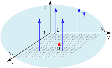
Figure 1: Schematic diagram of the probing technique discussed in this paper. A charged spinless particle confined on a finite two-dimensional square lattice is placed in a region subject to a locally transverse magnetic field. The presence of the magnetic field alters the eigenvectors and the spectra of the Hamiltonian, such that information about the value of the field may be retrieved by performing measurement on the particle in its ground state. We derive the ultimate achievable precision and also assess the performance of coarse-grained position measurement, showing that it may be employed to realize nearly optimal estimation strategies.

As already mentioned above, in order to assess and compare different estimation schemes, we employ the QFI as figure of merit. This is a proper choice, since we address situations where some a priori information about the field is available, and a local estimation approach is thus appropriate to optimize the detection scheme. We evaluate the QFI through the ground state fidelity and link it to the physical properties of the system. In particular, we observe a relationship between the structure of the Hamiltonian spectrum and the QFI obtained from a ground state measurement, thus linking precision to the spectral properties of the probe. We also introduce a possible strategy to optimize this estimation process by using a space-dependent magnetic field.

The paper is structured as follows. In Section II we introduce the system, i.e. its Hamiltonian and the shape of the orthogonal static magnetic field. In Section III we introduce the theoretical framework of our measurements, i.e. we provide the main results and concepts of quantum estimation theory (QET) used in this work and we study the feasibility of a position measurement, whereas in Section IV we show the reason why this system is of potential use as magnetometer by focusing on ground state measurements. Section V closes the paper with some concluding remarks, and possible outlooks.

II The probing system

The quantum probe consists of a charged spinless particle on a finite 2D square lattice in the presence of a locally transverse magnetic field. The lattice lays on the $xy$-plane and the magnetic field in the neighbouring region is parallel to the $z$-axis. The finiteness of the system is implemented by preventing the particle from hopping beyond the boundaries (see Fig. 2). We set $\hbar=q=d=1$, where $\hbar$ is the reduced Planck constant, $q$ the electric charge and $d$ the lattice constant. The lattice has size $N_{x}\times N_{y}$, where we denote, respectively, with $N_{x}$ and $N_{y}$ the total number of sites in the $x$- and $y$-direction. We set $N_{x}=N_{y}=31$, since a $(2n+1)\times(2n+1)$ lattice has a properly defined center in $(n+1,n+1)$ (i.e. having $n$ sites before and after itself along the two orthogonal directions).

In the following we first discuss the details of the magnetic field and then the Hamiltonian of this system. In particular, we briefly describe the configurations we are going to consider, with emphasis on the constraints arising out of the particular shape chosen for the inhomogeneous magnetic field. A homogeneous magnetic field orthogonal to the $xy$-plane

$$\mathbf{B}=B_{0}\,\hat{\mathbf{k}}$$ (1)

can be obtained by choosing the symmetric gauge with the vector potential defined as

$$\mathbf{A}=\frac{B_{0}}{2}(-(y-y_{0}),(x-x_{0}),0),$$ (2)

where the magnetic field magnitude $B_{0}$ is constant, and $(x_{0},y_{0})$ are the coordinates of the lattice center.

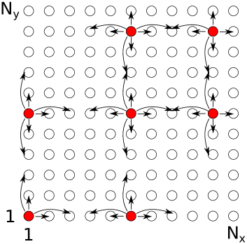
Figure 2: The finitiness of the system, i.e. of the $N_{x}\times N_{y}$ square lattice, is encoded in the allowed hopping paths, i.e. in the fact that the particle cannot jump beyond the boundaries. In this work we consider the hopping up to next-nearest neighbors. Here are some relevant cases: in the middle of the lattice the hopping is allowed up to next-nearest neighbors in both the directions; at the boundaries the hopping beyond the ends is forbidden; in the second last site along either or both of the directions the hopping to nearest neighbors is preserved, while some paths towards next-nearest neighbors are forbidden.

We are also interested in the study of space-dependent magnetic fields. In particular, we will consider a magnetic field profile constant along one axis (e.g. $y$) and varying along the other, such that it reaches its maximum value in the middle of the lattice - sites of coordinates $(x_{0},y)$) -, as shown in Fig. 3. So, in order to get the desired magnetic field, we introduce a function

$$f(x)=\beta-\alpha\lvert x-x_{0}\rvert,$$ (3)

where $\alpha,\beta\in\mathbb{R}^{+}$, which leads to the following generalized expression for the vector potential:

$$\mathbf{A}=\frac{f(x,y)}{2}(-(y-y_{0}),(x-x_{0}),0).$$ (4)

According to this definition, the analytical expression of the magnetic field reads:

$$\mathbf{B}=(B_{0}-m_{x}\lvert x-x_{0}\rvert)\hat{\mathbf{k}},$$ (5)

where $m_{x}=3\alpha/2$ is the gradient and $B_{0}=\beta$ is the maximum value of the magnitude of the magnetic field assumed on the sites of coordinates $(x_{0},y)$, i.e. in the middle of the lattice. Notice that, having chosen a $(2n+1)\times(2n+1)$ lattice, the magnitude of the magnetic field at the boundaries of the lattice (along $x$) is the same. It should be emphasised that such a magnetic field profile is fully characterized by the two parameters $B_{0}$ and $m_{x}$, the homogeneous magnetic field being just a special case for $m_{x}=0$.

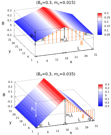
Figure 3: (Top panel) Spatial dependence of the inhomogeneous magnetic field described in Eq. (5). It reaches its maximum value $B_{0}$ in the middle of the lattice, i.e. in the sites of coordinates $(x_{0},y)$. By moving away from it, it decreases linearly (slope $\pm m_{x}$, with $m_{x}=\tan(\alpha)$) along the $x$-direction, while it is constant along the $y$ one. The couple of parameters $(B_{0},m_{x})$ must be chosen in a way that the reversal of $\mathbf{B}$ (bottom panel), occurring when Eq. (7) holds, is avoided.

The spatial dependence of the inhomogenous magnetic field and the magnetic length play a crucial role in defining the interval of fields investigated. The upper limit is given by the magnetic length $l_{B}$, which is the fundamental characteristic length scale for any quantum phenomena in the presence of a magnetic field Tong (2016), and which is defined as follows:

$$l_{B}:=\sqrt{\frac{\hbar}{qB}}.$$ (6)

According to our units ($\hbar=q=d=1$) the magnetic length reads $l_{B}=B^{\nicefrac{{-1}}{{2}}}$. For $B>1$ the magnetic length becomes smaller than the lattice constant $d$, hence we consider only $B_{0}<1$. The lower limit, instead, is due to the need of avoiding the reversal of the magnetic field (see bottom panel of Fig. 3), which occurs when

$$B_{0}<m_{x}L,$$ (7)

where $L:=\max_{x}(\lvert x-x_{0}\rvert)=15$, in our system. In conclusion, we consider $B_{0}\in\left[m_{x}L,1\right]$.

The Hamiltonian describing a charged spinless particle in an electromagnetic field reads Landau and Lifshitz (1977):

$$\mathcal{H}=\frac{1}{2m}\left(\mathbf{p}-q\mathbf{A}\right)^{2}+q\phi,$$ (8)

where $q$ is the charge and $m$ the mass of the particle, $\phi$ and $\mathbf{A}$ are the scalar and vector potential respectively. The former is set to zero in this work since we are interested in having the magnetic field only. These potentials are defined by the following relations:

$$\mathbf{E} =-\gradient{\phi}-\partialderivative{\mathbf{A}}{t},$$ (9)

$$\mathbf{B} =\curl{\mathbf{A}},$$ (10)

where $\mathbf{E}$ and $\mathbf{B}$ are the electric and magnetic field, respectively. In order to have a magnetic field parallel to the $z$-axis, one can choose the vector potential $\mathbf{A}=(A_{x}(x,y),A_{y}(x,y),0)$.

The Hamiltonian describing such a system on a lattice is obtained by introducing a space discretization of Eq. (8), i.e. by discretizing the $xy$-plane into a square lattice. Since we are considering a lattice, we have to express derivatives with finite difference and this, in turn, corresponds to discretizing the space. We adopt a five-point finite difference formula Abramowitz and Stegun (1964) to express derivatives and, according to this choice, we are able to write down the analytical expression of the resulting Hamiltonian:

$$\mathcal{H} =-J\sum_{j,k=1}^{N_{x},N_{y}}\left\{\vphantom{\frac{1}{1}}\left[-5-\left({A_{j,k}^{x}}^{2}+{A_{j,k}^{y}}^{2}\right)\right]\outerproduct{j,k}{j,k}+\right.$$

$$-\frac{1}{12}\left[\vphantom{A_{j,k}^{y}}1+i\left(A_{j-2,k}^{x}+A_{j,k}^{x}\right)\right]\outerproduct{j,k}{j-2,k}+$$

$$+\frac{2}{3}\left[\vphantom{A_{j,k}^{y}}2+i\left(A_{j-1,k}^{x}+A_{j,k}^{x}\right)\right]\outerproduct{j,k}{j-1,k}+$$

$$+\frac{2}{3}\left[\vphantom{A_{j,k}^{y}}2-i\left(A_{j+1,k}^{x}+A_{j,k}^{x}\right)\right]\outerproduct{j,k}{j+1,k}+$$

$$-\frac{1}{12}\left[\vphantom{A_{j,k}^{y}}1-i\left(A_{j+2,k}^{x}+A_{j,k}^{x}\right)\right]\outerproduct{j,k}{j+2,k}+$$

$$-\frac{1}{12}\left[1+i\left(A_{j,k-2}^{y}+A_{j,k}^{y}\right)\right]\outerproduct{j,k}{j,k-2}+$$

$$+\frac{2}{3}\left[2+i\left(A_{j,k-1}^{y}+A_{j,k}^{y}\right)\right]\outerproduct{j,k}{j,k-1}+$$

$$+\frac{2}{3}\left[2-i\left(A_{j,k+1}^{y}+A_{j,k}^{y}\right)\right]\outerproduct{j,k}{j,k+1}+$$

$$\left.-\frac{1}{12}\left[1-i\left(A_{j,k+2}^{y}+A_{j,k}^{y}\right)\right]\outerproduct{j,k}{j,k+2}\right\},$$ (11)

where $\ket{j,k}$ - with $j=1,\ldots,N_{x}$ and $k=1,\ldots,N_{y}$ - denotes a position eigenvector, i.e. a state describing the particle localized on the site of coordinates $(jd,kd)$. Analogously, the components of the vector potential have to be intended as $A^{x(y)}_{j,k}=A^{x(y)}(jd,kd)$. The parameter $J$ is a constant and, after restoring the fundamental constants and parameters, it reads $J=\hbar^{2}/(2md^{2})$. We set $m=1/2$ and thus $J=1$.

The expression of $\mathcal{H}$ in Eq. (11) fits the usual interpretation of the Hamiltonian describing a CTQW Hines and Stamp (2007); De Raedt and Michielsen (1994). In this case it would describe the CTQW of a charged spinless particle on a finite 2D square lattice. The hopping of the walker is described by projectors onto different position eigenvectors. For example $\outerproduct{j,k}{j-1,k}$ is the tunneling from site $(j-1,k)$ to site $(j,k)$, and the associated tunneling amplitude depends on the vector potential. Moreover, the on-site energy (associated to projectors onto the same state) depends quadratically on the magnitude of the vector potential.

III The estimation procedure

In this section we introduce some theoretical tools to optimize the estimation of a parameter, say $\lambda$, which, in our case, is the magnitude $B_{0}$ of the (in)homogeneous magnetic field. Let us consider the family $\rho_{\lambda}$ of the possible states of our probe, labeled by the parameter $\lambda$, which constitutes the quantity to be estimated. The main goal is to infer the value of $\lambda$ by measuring some observable quantity over $\rho_{\lambda}$. To this aim one performs repeated measurements on identical preparations of the system and then processes the outcomes $(x_{1},x_{2},\dots,x_{M})$ in order to obtain an estimator for the parameter, $\hat{\lambda}=\hat{\lambda}(x_{1},x_{2},\dots,x_{M})$. The figure of merit usually adopted to assess the precision of an estimator is the variance $\operatorname{Var}(\lambda)=\mathbb{E}_{\lambda}[\hat{\lambda}^{2}]-\mathbb{E}_{\lambda}[\hat{\lambda}]^{2}$. In case of unbiased estimators, the variance is equal to the mean square error of the estimator, $V(\lambda)=\mathbb{E}_{\lambda}[(\hat{\lambda}-\lambda)^{2}]$. The Cramèr-Rao inequality gives an upper bound for the estimator variance

$$V(\lambda)\geq\frac{1}{MF(\lambda)},$$ (12)

where $M$ is the number of measurements and $F(\lambda)$ is the Fisher information (FI) defined as

$$F(\lambda)=\int dx\,p(x|\lambda)\left[\partial_{\lambda}\ln p(x|\lambda)\right]^{2},$$ (13)

where $p(x|\lambda)$ is the conditional probability of obtaining the outcome $x$ when the value of the parameter is $\lambda$. In quantum mechanics, according to the Born rule, such conditional probability is written as $p(x|\lambda)=\Tr\left[\Pi_{x}\rho_{\lambda}\right]$, where $\{\Pi_{x}\}$, $\int dx\,\Pi_{x}=\mathbb{I}$, are the elements of a positive operator-valued measure. In order to achieve the ultimate bound to precision as posed by quantum mechanics, the FI must be maximized over all possible measurements. This procedure can be done by introducing the Symmetric Logarithmic Derivative (SLD) $L_{\lambda}$ as the operator satisfying the equation $L_{\lambda}\rho_{\lambda}+\rho_{\lambda}L_{\lambda}=2\partial_{\lambda}\rho_{\lambda}$. The ultimate bound of the precision of any estimator is expressed by the quantum Cramèr-Rao bound

$$V(\lambda)\geq\frac{1}{MH(\lambda)},$$ (14)

where $H(\lambda)=\Tr[\rho_{\lambda}L_{\lambda}^{2}]$ is the so-called quantum Fisher information. Indeed, it can be proved that the FI of any quantum measurement is bound by the QFI, i.e.

$$F(\lambda)\leq H(\lambda).$$ (15)

When the condition $F(\lambda)=H(\lambda)$ holds, the measurement is said to be optimal. An optimal (projective) measure is given by the spectral measure of the SLD which, however, may not easy to implement practically.

In this work we deal with pure states and we are interested in estimating a single parameter. This leads to the following simple expression for the QFI:

$$H(\lambda)=\frac{8\left(1-|\langle\psi_{\lambda}|\psi_{\lambda+\delta\lambda}\rangle|\right)}{(\delta\lambda)^{2}}.$$ (16)

For a given $\lambda$, a large value of the QFI implies that the quantum states $|\psi_{\lambda}\rangle$ and $|\psi_{\lambda+\delta\lambda}\rangle$ are statistically more distinguishable than the same pair of states for a value $\lambda$ corresponding to smaller QFI. This confirms the intuitive picture where optimal estimability (diverging QFI) is reached when quantum states are sent far apart upon infinitesimal variations of the parameter.

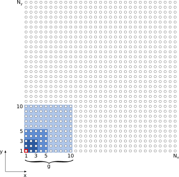
Figure 4: A coarse-grained position within the $N_{x}\times N_{y}=31\times 31$ square lattice is defined as a $(g\times g)$-sized cluster of sites, where $g=1,3,5,10$.

Besides the SLD, the natural choice for an observable providing information about the field is the position. We consider the two observables $X$ and $Y$ such that

$$X|j,k\rangle=jd\,|j,k\rangle Y|j,k\rangle=kd\,|j,k\rangle,$$ and (17)

where $d$ is the lattice constant and $\{|j,k\rangle\}$ is the orthonormal basis of the position eigenvectors. We measure the compatible pair of observables $(X,Y)$ and, in order to assess the performance, we evaluate the ratio

$$R(\lambda)=\frac{F(\lambda)}{H(\lambda)}\in[0,1]$$ (18)

between the position FI $F$ and the QFI $H$, respectively given in Eq. (13) and Eq. (16), in the light of Eq. (15). This ratio tells us how much the FI of a given measurement is close to the QFI, which is achieved when $R=1$. We perform a ground state measurement, then the probabilities entering Eq. (13) are straightforwardly given by the square modulus of the projections of the ground state onto the position eigenvectors. The Hamiltonian in Eq. (11) is already written in the basis of position eigenvectors, thus the components of the ground state are actually the projections we need.

In addition, we investigate the performance of coarse-grained position measurement, i.e. whether position measurement is robust when the resolution of the measurement does not permit to measure the probability associated to a single site of the lattice. To this purpose, we define square grains of size $g\times g$, where $g=1,3,5,10$ denotes the number of sites forming the side of the cluster (see Fig. 4). We keep as reference $H$ and compute $F$ at different $g$ by rewriting Eq. (13) in terms of grain probabilities rather than site probabilities. This may done as follows: let us denote a generic site as $s:=(j,k)$ and a grain, i.e. a cluster of sites, of size $g\times g$ as $G_{g}$. Notice that these clusters are disjoint ($G_{g}\cap G_{g}^{\prime}=\emptyset$). Then we compute the FI as

$$F_{g}(\lambda)=\sum_{G_{g}}P(G_{g}|\lambda)\Big{[}\partial_{\lambda}\ln P(G_{g}|\lambda)\Big{]}^{2},$$ (19)

where

$$P(G_{g}|\lambda)=\sum_{s\in G_{g}}p(s|\lambda)$$ (20)

is the grain probability and $p(s|\lambda)$ is the site probability, i.e. the conditional probability of finding the walker in the site $s$ when the parameter takes the value $\lambda$. Clearly, for $g=1$ grain probability corresponds to site probability.

IV Ground state quantum magnetometry

In this section we focus on ground state measurements in order to assess the behavior of this system as quantum magnetometer, i.e. as a probe to estimate the magnitude of the magnetic field acting on it. To this aim we compute the QFI via Eq. (16): the parameter $\lambda$ to be estimated is the magnetic field magnitude $B_{0}$, whereas $\ket{\psi_{\lambda}}$ and $\ket{\psi_{\lambda+\delta\lambda}}$ are the system ground states corresponding to magnetic field magnitudes $B_{0}$ and $B_{0}+\delta B>B_{0}$, respectively.

IV.1 Homogeneous magnetic field

In order to understand whether our system is of potential use as quantum magnetometer, we first consider a static homogeneous magnetic field ($m_{x}=0$). We compute the QFI for different values of $B_{0}$, and also the position FI to assess its performance and to study which values of the parameter, if any, can be better estimated (see top panel of Fig. 5).

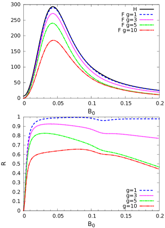
Figure 5: Quantum Fisher information $H$, position Fisher information $F$ (at different grain size $g$) (top panel) and their ratio $R=F/H$ (bottom panel) as a function of the magnitude $B_{0}$ of the static homogeneous magnetic field ($m_{x}=0$).

The first observation is that the QFI (solid black line $H$) is non-vaninshing in the whole magnetic field interval considered, showing that estimation of the field may be indeed obtained from ground state measurement. Then, we notice that even if the position FI (dashed colored lines $F$) is smaller than the QFI, it has the same order of magnitude. In particular, it decreases for increasing the grain size $g$, but it still preserves a structure analogous to that of the QFI. The behavior of the FI is more clearly depicted in bottom panel of Fig. 5, where we see that the ratio $R=F/H$ moderately decreases as the grain size increases. Yet, for $g=1$, $F$ overlaps very well to the curve of $H$, as proved by the fact that the ratio $R$ is close to $1$ in the whole interval of $B_{0}$ considered.

In Fig. 6 we illustrate the behavior of the QFI: it is dependent on the magnetic field and the region of high QFI suggests that some values can be estimated more efficiently than the others. Indeed, as it can be seen from Eq. (16), high values of QFI denote that a slight change in the parameter of interest greatly affects the ground state, in a way that $|\langle\psi_{\lambda+\delta\lambda}|\psi_{\lambda}\rangle|<1$. The same interval of $B_{0}$ characterized by a high QFI is also where the system partial energy spectrum, i.e. the lowest Hamiltonian eigenvalues, shows the more complex dependence on $B_{0}$.

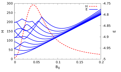
Figure 6: Quantum Fisher information $H$ (dashed red line) and lower-energy spectrum (solid blue line) as a function of the magnitude $B_{0}$ of the static homogeneous magnetic field ($m_{x}=0$).

IV.2 Inhomogeneous magnetic field

The interesting features shown by the QFI for a static homogeneous magnetic field ($m_{x}=0$) are further investigated here by considering a static inhomogeneous magnetic field ($m_{x}>0$). In this case, as we notice in top panel of Fig. 7, the QFI (solid black line $H$) is still non-null within the whole interval of magnetic field considered. The position FI does not follow the behavior of the QFI for low $B_{0}$ but it does it in correspondence of the peak of the QFI. Also in this case we show the ratio $R=F/H$ in the bottom panel of Fig. 7.

As it may be seen looking at Fig. 8, the QFI peak occurs for the value of $B_{0}$ such that the lowest energy eigenvalues present an avoided crossing phenomenon, such that the behavior of the QFI may be interpreted in terms of the structure of a two-level effective system. Indeed, in systems with parameter-dependent Hamiltonians, small perturbations may induce relevant changes in the ground state of the system, and this behavior is emphasised in the presence of level anticrossing. Summarizing from Ghirardi et al. (2018), we have that for a two-level system with (generic) Hamiltonian of the form

$${\cal H}_{2}=\omega_{0}\sigma_{0}-\Delta(\lambda)\sigma_{3}+\gamma(\lambda)\sigma_{1}\,,$$

where $\sigma_{k}$ (with $k=0,\ldots,3$) denote the Pauli matrices, the QFI $H(\lambda)$ may be written as

$$H(\lambda)=16\,\left(\frac{\Delta}{h_{+}-h_{-}}\right)^{4}\left[\partial_{\lambda}\left(\gamma/\Delta\right)\right]^{2}\,,$$ (21)

where $h_{\pm}$ are the eigenvalues of ${\cal H}_{2}$.

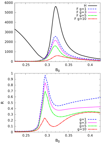
Figure 7: Quantum Fisher information $H$, position Fisher information $F$ (at different grain size $g$) (top panel) and their ratio $R=F/H$ (bottom panel) as a function of the magnitude $B_{0}$ (value in the lattice center) of the static inhomogeneous magnetic field ($m_{x}=0.015$).

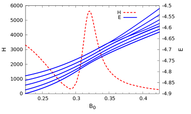
Figure 8: Quantum Fisher information $H$ (dashed red line) and lower-energy spectrum (solid blue line) as a function of the magnitude $B_{0}$ (value in the lattice center) of the static inhomogeneous magnetic field ($m_{x}=0.015$).

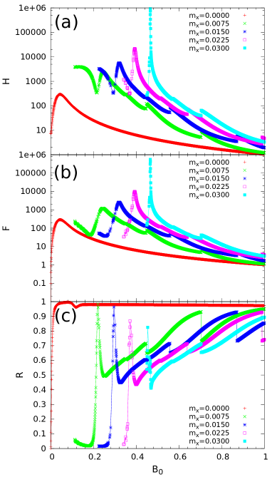
Figure 9: (a) Quantum Fisher information $H$, (b) position Fisher information $F$ at grain size $g=1$ and (c) their ratio $R=F/H$ at varying magnitude $B_{0}$ (value in the lattice center) of the static inhomogeneous magnetic field for different values of the gradient $m_{x}$.

In Fig. 9 we plot the QFI as a function of $B_{0}$ for different values of the gradient $m_{x}$. These results clearly show that for any value of the parameter $B_{0}$ to be estimated, there is a gradient value $m_{x}$ which maximizes the QFI. Therefore estimability performances can be enhanced by a proper choice of $m_{x}$. In other words, the system may actually be employed as a quantum magnetometer, since it allows to estimate the magnetic field magnitude $B_{0}$ starting from a ground state measurement, which can be optimized by choosing the optimal gradient $m_{x}$. We stress again that the estimation of $B_{0}$ and the prior knowledge of $m_{x}$ are enough to fully describe the magnetic field shape. We notice here that the complentary problem of gradient magnetometry has been recently addressed Apellaniz et al. (2018) with atomic ensembles, showing that achieving the precision bounds requires the knowledge of the homogeneous part of the field. The correlation between the QFI maxima and the structures of the energy spectrum can be exploited by considering the possibility of obtaining informations about the energy spectrum starting from the QFI, or vice versa by investigating the energy spectrum in order to gain informations about the QET properties of the system.

V Conclusions

In this work, we have studied a charged spinless particle on a finite 2D square lattice in the presence of a locally transverse magnetic field. The Hamiltonian has been derived from a spatial discretization of the Hamiltonian of the corresponding system in a plane, and the time-independent Schrödinger equation has been solved exactly by numerical diagonalization for a lattice size $31\times 31$. Our focus has been on the potential use of the quantum features of this system as quantum magnetometer. In particular, we have analyzed its performance in the estimation of a transverse magnetic field, either homogeneous or inhomogeneous, by performing measurements on the system’s ground state.

Our results show that the system is of interest from the metrological standpoint: the ground state QFI for the magnetic field is non-negligible in a large range of configurations. We have first seen this behavior for the case of a homogeneous magnetic field, and then for a space-dependent magnetic field. In particular, we have found that the QFI shows peaks at specific values of the magnetic field and of its gradient, making it possible to optimize the estimation strategy by properly tuning the value of the latter. In order to gain insight into the origin of the QFI peaks, we have analyzed the structure of the Hamiltonian spectra, and found that the relation between the QFI peaks and the values of magnetic field at which they occur may be understood in terms of avoided crossing phenomena between the two lowest Hamiltonian eigenvalues.

We have also studied the performance of position measurements. In the case of ground state measurements the corresponding FI provides a quite good approximation to the QFI, showing an analogous peak structure. In particular, for a homogeneous magnetic field the FI overlaps very well to the QFI. For an inhomogeneous magnetic field the FI reproduces the behavior of QFI at least in the neighborhood of QFI peak. Concerning robustness, we have found that if one is not able to perform measurements at site resolution, but have access to coarse-grained measurement only at level of clusters of sites, the FI decreases as the grain size increases. On the other hand, the FI has the same order of magnitude of the QFI and preserves a peak structure analogous to QFI, proving the robustness of this kind of measurement.

In conclusion, our results show that effective quantum sensing of magnetic fields is possible using a charged spinless particle on a finite two-dimensional lattice. In particular, ultimate bounds to precision may be approached by position measurement on the ground state of the system, which is also robust against coarse-graining, i.e. reduction of resolution.