The coherent structure of the kinetic energy transfer in shear turbulence

Abstract

The cascade of energy in turbulent flows, i.e., the transfer of kinetic energy from large to small flow scales or vice versa (backward cascade), is the cornerstone of most theories and models of turbulence since the 1940s. Yet, understanding the spatial organisation of kinetic energy transfer remains an outstanding challenge in fluid mechanics. Here, we unveil the three-dimensional structure of the energy cascade across the shear-dominated scales using numerical data of homogeneous shear turbulence. We show that the characteristic flow structure associated with the energy transfer is a vortex shaped as an inverted hairpin followed by an upright hairpin. The asymmetry between the forward and backward cascade arises from the opposite flow circulation within the hairpins, which triggers reversed patterns in the flow.

1 Introduction

Turbulence exhibits a wide range of flow scales, whose interactions are far from understood (Cardesa et al., 2017). These interactions are responsible for the cascading of kinetic energy from large eddies to the smallest eddies, where the energy is finally dissipated (Richardson, 1922; Obukhov, 1941; Kolmogorov, 1941, 1962; Aoyama et al., 2005; Falkovich, 2009). Given the ubiquity of turbulence, a deeper understanding of the energy transfer among the flow scales would enable significant progress to be made across various fields ranging from combustion (Veynante & Vervisch, 2002), meteorology (Bodenschatz, 2015), and astrophysics (Young & Read, 2017) to engineering applications of external aerodynamics and hydrodynamics (Sirovich & Karlsson, 1997; Hof et al., 2010; Marusic et al., 2010; Kühnen et al., 2018; Ballouz & Ouellette, 2018). In the vast majority of real-world scenarios, turbulence is accompanied by an abrupt increase of the mean shear in the vicinity of the walls due the friction induced by the latter. These friction losses are responsible for roughly 10% of the electric energy consumption worldwide (Kühnen et al., 2018). Moreover, the success of large-eddy simulation (LES), which is an indispensable tool for scientific and engineering applications (Bose & Park, 2018), lies in its ability to correctly reproduce energy transfer among scales. Hence, a comprehensive analysis of the interscale energy transfer mechanism is indispensable for both physical understanding of turbulence and for conducting high-fidelity LES.

Substantial efforts have been directed toward the statistical characterisation of interscale kinetic energy transfer using flow data acquired either by simulations or experimental measurements (e.g., Natrajan & Christensen, 2006; Kawata & Alfredsson, 2018). Several works have further examined the cascading process conditioned to selected regions of the flow, mainly motivated by the fact that the interscale energy transfer is highly intermittent both in space and time (see Piomelli et al., 1991; Domaradzki et al., 1993; Cerutti & Meneveau, 1998; Aoyama et al., 2005; Ishihara et al., 2009; Dubrulle, 2019, and references therein). By conditionally averaging the flow, previous works have revealed that kinetic energy fluxes entail the presence of shear layers, hairpin vortices, and fluid ejections/sweeps. However, further progress in the field has been hindered by the scarcity of flow information, which has been limited to a few velocity components and two spatial dimensions. Consequently, less is known about the underlying three-dimensional structure of the energy transfer, which is the focus of this work.

Härtel et al. (1994) conducted one of the earliest numerical investigations on kinetic energy fluxes and their accompanying coherent flow structures. Their findings showed that the backward transfer of energy is confined within a near-wall shear layer. In a similar study, Piomelli et al. (1996) proposed a model comprising regions of strong forward and backward energy transfer paired in the spanwise direction, with a quasi-streamwise vortex in between. This view was further supported by an LES study on the convective planetary boundary layer (Lin, 1999). The previous works pertain to the energy transfer across flow scales under the influence of the mean shear, which is the most relevant case from the engineering and geophysical viewpoints. Still, it is worth mentioning that the inertial energy cascade has been classically ascribed to the stretching exerted among vortices at different scales in isotropic turbulence (Goto et al., 2017; Motoori & Goto, 2019), although recent works have debated this view in favour of strain-rate self-amplification as the main contributor to the energy transfer among scales (Carbone & Bragg, 2019). The reader is referred to Alexakis & Biferale (2018) for an unified and exhaustive review of the different energy transfer mechanisms.

On the experimental side, Porté-Agel and collaborators (Porté-Agel et al., 2002, 2001; Carper & Porté-Agel, 2004) performed a series of studies in the atmospheric boundary layer. They conjectured that regions of intense forward and backward cascades organised around the upper trailing edge and lower leading edge of a hairpin, respectively. Later investigations using particle-image velocimetry in turbulent boundary layers with smooth walls (Natrajan & Christensen, 2006) and rough walls (Hong et al., 2012) corroborated the presence of counter-rotating vertical vorticity around regions of intense kinetic energy transfer, consistent with Carper & Porté-Agel (2004). More recent studies of the mixing layer induced by Richtmyer–Meshkov instability (Liu & Xiao, 2016) have also revealed flow patterns similar to those described above.

Previous numerical and experimental studies have helped advance our understanding of the spatial structure of energy transfer; however, they are limited to only two dimensions. With the advent of the latest simulations and novel flow identification techniques (e.g. Del Álamo et al., 2004; Lozano-Durán et al., 2012; Lozano-Durán & Jiménez, 2014; Dong et al., 2017; Osawa & Jiménez, 2018), the three-dimensional characterisation of turbulent structures is now achievable to complete the picture. In the present study, we shed light on the three-dimensional flow structure associated with regions of intense energy fluxes in the most fundamental set-up for shear turbulence.

The present work is organised as follows. The numerical database and the filtering approach to study the energy transfer in homogeneous shear turbulence is described in §2. The results are presented in §3, which is further subdivided into two parts. In §3.1, we show the spatial organisation of the flow structures responsible for the forward and backward energy cascade. The coherent flow associated with both energy cascades is analysed in §3.2. Finally, conclusions are offered in §4.

2 Numerical experiment and filtering approach

2.1 Database of homogeneous shear turbulence

We examine data from the direct numerical simulation (DNS) of statistically stationary, homogeneous, shear turbulence (SS-HST) from Sekimoto et al. (2016). The flow is defined by turbulence in a doubly periodic domain with a superimposed linear mean shear profile (Champagne et al., 1970). This configuration, illustrated in figure 1, is considered the simplest anisotropic flow, sharing the natural energy-injection mechanism of real-world shear flows. Hence, our numerical results are utilised as a proxy to gain insight into the physics of wall-bounded turbulence without the complications of the walls (Dong et al., 2017). The Reynolds number of the simulation based on the Taylor microscale is $Re_{\lambda}=q^{2}(5/3\nu\varepsilon)^{1/2}\approx 100$ (with $q^{2}$ and $\varepsilon$ the kinetic energy and dissipation, respectively), which is comparable to that in the logarithmic layer of wall-bounded turbulence at a friction Reynolds number of $Re_{\tau}\approx 2000$.

Hereafter, fluctuating velocities are denoted by $u$, $v$, and $w$ in the streamwise ($x$), vertical ($y$), and spanwise ($z$) directions, respectively. The mean velocity vector averaged over the homogeneous directions and time is $(U,V,W)=(Sy,0,0)$, where $S$ is the constant mean shear rate. Occasionally, we use subscripts $1$, $2$, and $3$ to refer to the streamwise, vertical, and spanwise directions (or velocities), respectively, in which case repeated indices imply summation. Details of the simulation are listed in table 1.

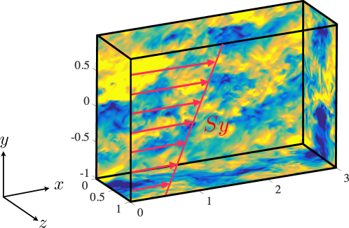
Figure 1: Schematic of the computational domain. $S$ is the superimposed mean shear. The read arrows are the streamwise mean velocity profile, $U=Sy$. The colours represent the magnitude of streamwise fluctuating velocity, $u$, in the range $[-1,1]$ from yellow to blue. The streamwise, vertical, and spanwise coordinates are $x$, $y$, and $z$, respectively. The lengths are normalised with the spanwise size of the domain. The velocities are normalised with the friction velocity defined as $u_{\tau}^{2}=|\nu S-\langle uv\rangle|$. The flow is periodic in $x$ and $z$. Periodicity is enforced at the upper and lower boundaries for points that are uniformly shifted in the $x$ consistently with the superimposed mean shear.

$Re_{\lambda}$	$A_{xz}$	$A_{yz}$	$\Delta x/\eta$	$\Delta y/\eta$	$\Delta z/\eta$	$L_{c}/\eta$	$L_{z}/\eta$
104	3	2	1.6$\pm$0.18	1.0$\pm$0.12	1.0$\pm$0.12	36	366

Table 1: Simulation parameters for the DNS of SS-HST used in this paper. $Re_{\lambda}=q^{2}(5/3\nu\varepsilon)^{1/2}$ is the Reynolds number based on the Taylor microscale ($q^{2}$ and $\varepsilon$ are the kinetic energy and dissipation, respectively); $A_{xz}=L_{x}/L_{z}$ and $A_{yz}=L_{y}/L_{z}$ are the box aspect ratios of the computational domain; $\Delta x/\eta$, $\Delta y/\eta$ and $\Delta z/\eta$ are the grid resolutions in terms of the average Kolmogorov length-scale $\eta$, with their standard deviations due to intermittency. $\Delta x$ and $\Delta z$ are computed from the number of Fourier modes before dealiasing; $L_{c}$ is the Corrsin length-scale defined as $L_{c}=\sqrt{\varepsilon/S^{3}}$.

The code integrates in time the equation for the vertical vorticity $\omega_{y}$ and for the Laplacian of $v$. The spatial discretization is dealiased Fourier spectral in the two periodic directions, and compact finite differences with spectral-like resolution in $y$. The Navier–Stokes equations of motion, including continuity, are reduced to the evolution equations for $\phi=\nabla^{2}v$ and $\omega_{y}$ (Kim et al., 1987) with the advection by the mean flow explicitly separated,

$$\dfrac{\partial\omega_{y}}{\partial t}+Sy\dfrac{\partial\omega_{y}}{\partial x}=h_{g}+\nu\nabla^{2}\omega_{y},\qquad\dfrac{\partial\phi}{\partial t}+Sy\dfrac{\partial\phi}{\partial x}=h_{v}+\nu\nabla^{2}\phi,$$ (1)

where $\nu$ is the kinematic viscosity. Defining $\textbf{{H}}=\textbf{{u}}\times\boldsymbol{\omega}$,

$$h_{g}\equiv\dfrac{\partial H_{x}}{\partial z}-\dfrac{\partial H_{z}}{\partial x}-S\dfrac{\partial v}{\partial z},\qquad h_{v}\equiv-\dfrac{\partial}{\partial y}\left(\dfrac{\partial H_{x}}{\partial x}+\dfrac{\partial H_{z}}{\partial z}\right)+\left(\dfrac{\partial^{2}}{\partial{x}^{2}}+\dfrac{\partial^{2}}{\partial{z}^{2}}\right)H_{y}.$$ (2)

In addition, the governing equation for $\langle\textbf{{u}}\rangle_{xz}$ are

$$\dfrac{\partial\langle u\rangle_{xz}}{\partial t}=-\dfrac{\partial\langle uv\rangle_{xz}}{\partial y}+\nu\dfrac{\partial^{2}\langle u\rangle_{xz}}{\partial{y}^{2}},\qquad\dfrac{\partial\langle w\rangle_{xz}}{\partial t}=-\dfrac{\partial\langle wv\rangle_{xz}}{\partial y}+\nu\dfrac{\partial^{2}\langle w\rangle_{xz}}{\partial{y}^{2}},$$ (3)

where $\langle\cdot\rangle_{xz}$ denotes averaging on the homogeneous directions. The time stepping is a third-order explicit Runge–Kutta (Spalart et al., 1991) modified by an integrating factor for the mean-flow advection.

The spanwise, vertical, and spanwise size of the domain are denoted by $L_{x}$, $L_{y}$, and $L_{z}$, respectively. The numerical domain is periodic in $x$ and $z$, with boundary conditions in $y$ that enforce periodicity between uniformly shifting points at the upper and lower boundaries. More precisely, the boundary condition used is that the velocity is periodic between pairs of points in the top and bottom boundaries of the computational box, which are shifted in time by the mean shear (Baron, 1982; Schumann, 1985; Gerz et al., 1989; Balbus & Hawley, 1998). For a generic fluctuating quantity $g$,

$$g(t,x,y,z)=g(t,x+mStL_{y}+lL_{x},y+mL_{y},z+nL_{z}),$$ (4)

where $l,m$ and $n$ are integers. In terms of the spectral coefficients of the expansion,

$$g(t,x,y,z)=\sum_{k_{x}}\sum_{k_{z}}\widehat{g}(t,k_{x},y,k_{z})\exp[{\rm i}(k_{x}x+k_{z}z)],$$ (5)

the boundary condition becomes

$$\widehat{g}(t,k_{x},y,k_{z})=\widehat{g}(t,k_{x},y+mL_{y},k_{z})\exp[{\rm i}k_{x}mStL_{y}],$$ (6)

where $k_{i}=n_{i}\Delta k_{i}\,(i=x,z)$ are wavenumbers, $n_{i}$ are integers, and $\Delta k_{i}=2\pi/L_{i}$. This shifting boundary condition in $y$ avoids the periodic remeshing required by tilting-grid codes (Rogallo, 1981), and most of their associated enstrophy loss.

The simulations are characterised by the streamwise and vertical aspect ratios of the simulation domain, $A_{xz}=L_{x}/L_{z}=3$ and $A_{yz}=L_{y}/L_{z}=2$, and the Reynolds number $Re_{z}=SL_{z}^{2}/\nu$, where $\nu$ is the kinematic viscosity of the fluid. The velocities are normalised with the friction velocity defined as $u_{\tau}^{2}=|\nu S-\langle uv\rangle|$. Occasionally, we also use the Corrsin length, $L_{c}=(\varepsilon/S^{3})^{1/2}$, above which the mean shear dominates, where $\varepsilon$ is the mean rate of turbulence kinetic energy dissipation.

2.2 Definition of interscale kinetic energy transfer $\varPi$

The evolution equation for the $i$-th component of the velocity is

$$\frac{\partial u_{i}}{\partial t}+\frac{\partial u_{i}u_{j}}{\partial x_{j}}+Sy\frac{\partial u_{i}}{\partial x_{1}}=-Sv\delta_{i1}-\frac{1}{\rho}\frac{\partial p}{\partial x_{i}}+\nu\frac{\partial^{2}u_{i}}{\partial x_{j}\partial x_{j}}.$$ (7)

After low-pass filtering (7) using an isotropic Gaussian filter with filter size $r_{f}$, the equation for the filtered kinetic energy $\widetilde{k}=\widetilde{u}_{i}\widetilde{u}_{i}/2$ is given by

$$\frac{D\widetilde{k}}{Dt}=-S\widetilde{u}_{1}\widetilde{u}_{2}-J-\nu\frac{\partial\widetilde{u}_{i}}{\partial x_{i}}\frac{\partial\widetilde{u}_{i}}{\partial x_{i}}-\varPi_{\mathrm{MF}}-\varPi,$$ (8)

where $D(\cdot)/Dt$ is the material derivative and

$$\varPi_{\mathrm{MF}} = -[\widetilde{u_{i}U}-\widetilde{u}_{i}\widetilde{U}]\frac{\partial\widetilde{u}_{i}}{\partial x_{1}},$$ (9)

$$\varPi = -\tau_{ij}\frac{\partial\widetilde{u}_{i}}{\partial x_{j}}=-[\widetilde{u_{i}u_{j}}-\widetilde{u}_{i}\widetilde{u}_{j}]\frac{\partial\widetilde{u}_{i}}{\partial x_{j}},$$ (10)

$$J = \frac{\partial\widetilde{u}_{j}\widetilde{u}_{i}^{2}/2}{\partial x_{j}}+\frac{\partial\widetilde{Sy}\widetilde{u}_{i}^{2}/2}{\partial x}+\frac{1}{\rho}\frac{\partial\widetilde{p}\widetilde{u}_{i}}{\partial x_{i}}-\nu\frac{\partial}{\partial x_{j}}(\widetilde{u}_{i}\frac{\partial\widetilde{u}_{i}}{\partial x_{j}})+$$

$$+ \frac{\partial\widetilde{u}_{i}\widetilde{u_{i}u_{j}}}{\partial x_{j}}+\frac{\partial\widetilde{u}_{i}^{2}\widetilde{u}_{j}}{\partial x_{j}}+\frac{\partial\widetilde{u}_{i}\widetilde{Syu_{i}}}{\partial x}-\frac{\partial\widetilde{Sy}\widetilde{u}_{i}^{2}}{\partial x}.$$

$\varPi_{\mathrm{MF}}$ is the kinetic energy transfer due to the interaction between the filtered and mean flow, $\varPi$ is the transfer between flow scales, and $J$ is a spatial flux. We are concerned with $\varPi$, which represents the energy cascade. A positive value of $\varPi$ implies a transfer of energy from the large, unfiltered scales to the small, filtered scales (forward cascade), while negative values of $\varPi$ represent an opposite transfer (backward cascade). Filtered quantities are calculated using filter widths $r_{f}$ ranging from $23.3\eta$ in the viscous range to $80.0\eta$ in the inertial range, where $\eta$ is the Kolmogorov length scale. Since the large-scale structures in SS-HST are only slightly elongated in the streamwise direction (Dong et al., 2017), we utilise an spatially isotropic filter.

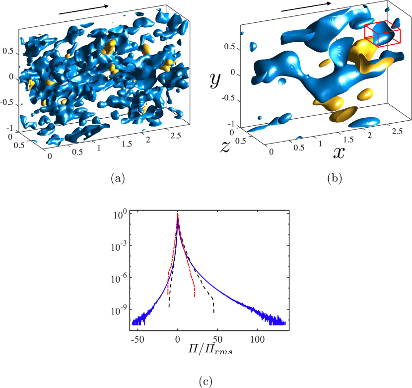
Figure 2: Instantaneous spatial distribution of regions of intense positive (blue) and negative (yellow) kinetic energy transfer $\varPi$ for filter sizes equal to (a) $r_{f}=23.3\eta$, and (b) $r_{f}=60\eta$. The arrow indicates the mean flow direction. The lengths are normalised with the spanwise size of the domain. The red box in panel (b) is the bounding box of an individual $\varPi^{+}$-structure identified by Eq. (12). (c) The p.d.f. of $\varPi$ for filter sizes equal to $23.3\eta$ (            ) and $60\eta$ (                   ). For comparison purposes, the figure also includes the additional filter width $r_{f}=5.8\eta$

(   ). Each p.d.f. is normalised by its standard deviation, $\varPi_{rms}$.

3 Results

Figures 2(a) and 2(b) show the instantaneous spatial distribution of regions of intense $\varPi$ for two filter widths, $r_{f}=23.3\eta$ and $r_{f}=60\eta$. Both forward and backward cascades coexist, as seen from the positive and negative regions of $\varPi$, although the forward cascade prevails. The spatial distribution of the fluxes is strongly inhomogeneous, with regions of intense energy transfer organised into intermittent spots (Piomelli et al., 1991; Domaradzki et al., 1993; Cerutti & Meneveau, 1998; Aoyama et al., 2005; Ishihara et al., 2009; Wu et al., 2017; Yang & Lozano-Durán, 2017). The probability density function (p.d.f.) of $\varPi$ (figure 2c) shows that the skewness factor of $\varPi$ decreases monotonically with the filter size (from 6.54 to 0.73), i.e., the cascade process becomes more symmetric at larger scales. The intensity of rare events also decreases dramatically as a function of the filter size.

In the following, we study the properties of three-dimensional structures of intense kinetic energy transfer. Individual structures are identified as a contiguous region in space satisfying

$$|\varPi(\boldsymbol{x})|>\alpha\varPi_{rms},$$ (12)

where $\boldsymbol{x}=(x,y,z)$, $\alpha>0$ is a threshold parameter, and $\varPi_{rms}$ is the standard deviation of $\varPi$. The value of $\alpha$ is chosen to be 1.0 based on a percolation analysis (Moisy & Jiménez, 2004); however, similar conclusions are drawn for $0.5<\alpha<2.0$. Connectivity is defined in terms of the six orthogonal neighbours in the Cartesian mesh of the DNS. By construction of Eq. (12), each individual structure belongs to either a region of forward or backward cascade, denoted by $\varPi^{+}$ and $\varPi^{-}$, respectively. Each structure is circumscribed within a box aligned to the Cartesian axes, whose streamwise, vertical, and spanwise sizes are denoted by $\Delta_{x}$, $\Delta_{y}$, and $\Delta_{z}$, respectively. The diagonal of the bounding box is given by $d=\sqrt{\Delta_{x}^{2}+\Delta_{y}^{2}+\Delta_{z}^{2}}$. The total number of structures used to compute the averaged flow field is of the order of $10^{4}$. Examples of instantaneous structures for two different filter sizes can be seen in figure 2(a) and figure 2(b). In the latter, one individual structure of $\varPi^{+}$ is enclosed within its bounding box (in red).

Prior to the investigation of the spatial organisation of the energy transfer, we discuss the amount of forward and backward cascade structures. Figure 3(a) shows the ratio of the total volume of backward cascade structures ($\sum_{i}V_{i}^{b}$) and the total volume of forward cascade structures ($\sum_{i}V_{i}^{f}$) for the different times employed in the analysis and for $r_{f}=60\eta$. The p.d.f. of the volume ratio $\sum_{i}V_{i}^{b}/\sum_{i}V_{i}^{f}$ is given in figure 3(b). The mean value is roughly 0.3, i.e., forward cascade events dominate, consistent with previous results in the literature (Piomelli et al., 1991; Aoyama et al., 2005). However, the ratio varies widely among instants, ranging from $2\times 10^{-3}$ to $4$, showing the time intermittency of the cascade.

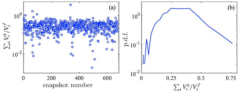
Figure 3: (a) The ratio of the total volume of backward cascade structures $\sum_{i}V_{i}^{b}$ and total volume of forward cascade structures $\sum_{i}V_{i}^{f}$ as a function of the snapshot used in the analysis. $V_{i}^{f}$ and $V_{i}^{b}$ are the volume of individual forward and backward structures, respectively, satisfying (12) with $\alpha=1.0$. The results are for filter width $r_{f}=60\eta$. (b) The p.d.f. of the volume ratio of backward and forward cascade structures from the data shown in panel (a).

3.1 Spatial organisation of the energy cascades

The spatial organisation of $\varPi^{+}$ and $\varPi^{-}$ is studied through the three-dimensional joint p.d.f., $p^{ij}$, of the relative distances between the individual structures of type $i$ and $j$, where $i$ and $j$ refer to either $\varPi^{+}$ or $\varPi^{-}$. The vector of relative distances is defined as

$$\boldsymbol{\delta}^{(ij)}=(\delta_{x},\delta_{y},\delta_{z})^{(ij)}=2\frac{\boldsymbol{x}_{c}^{(j)}-\boldsymbol{x}_{c}^{(i)}}{d^{(j)}+d^{(i)}},$$ (13)

where $\boldsymbol{x}_{c}^{(i)}$ is the centre of gravity of one individual structure, and $d^{(i)}$ is the diagonal length of its bounding box (highlighted in red in figure 2b). Only pairs of structures with similar sizes are considered in the computation of relative distances (Lozano-Durán et al., 2012; Osawa & Jiménez, 2018; Dong et al., 2017), in particular, those satisfying $1/2\leq d^{(j)}/d^{(i)}\leq 2$. We also take advantage of the spanwise symmetry of the flow, and $\delta_{z}$ is chosen to be positive toward the closest $j$-type structure.

Structures of $\varPi^{+}$ and $\varPi^{-}$ are preferentially organised size-by-size in the spanwise direction, as shown by the cross-section of $p^{\varPi^{+}\varPi^{-}}$ in figure 4(a). Except for $r_{f}=23.3\eta$, the distribution of $p^{\varPi^{+}\varPi^{-}}$ is bi-modal along the vertical direction, with peaks lying almost symmetrically at $\delta_{y}\approx\pm 0.25$. Conversely, structures of the same type are aligned in the streamwise direction with a separation of $|\delta_{x}|\approx 1$ and tilted by roughly $15^{\circ}$. The p.d.f.s in figure 4(b) are for $p^{\varPi^{+}\varPi^{+}}$ at $\delta_{z}=0$, but similar results are found for $p^{\varPi^{-}\varPi^{-}}$.

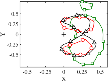
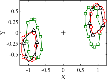
(a) (b)

Figure 4: Cross-sections of the three-dimensional joint p.d.f. of relative distances between the $\varPi$-structures for (a) $p^{\varPi^{+}\varPi^{-}}$ in the ($\delta_{z},\delta_{y}$) plane and (b) $p^{\varPi^{+}\varPi^{+}}$ in the ($\delta_{x},\delta_{y}$) plane. P.d.f.s are integrated over $\delta$=$\pm$0.2 normal to the plane of the plot. Contours contain the highest 15% of the data. In all the panels, the symbols are $\square$, $r_{f}=23.3\eta$; $\triangle$, $r_{f}=46\eta$; $\bigcirc$, $r_{f}=60\eta$; and $+$, $\delta_{x}=\delta_{y}=\delta_{z}=0$.

The p.d.f. and mean values of the diagonal length of individual $\varPi$-structures for different filter widths are plotted in figure 5(a) and figure 5(b), respectively. The results shows that the size of the structures are, on average, proportional to the filter width. Figure 5(a) shows some disparity between the p.d.f. of $d/L_{c}$ for $\varPi^{+}$ and $\varPi^{-}$, but the difference decreases with $r_{f}$, consistent with the skewness of the p.d.f. of $\varPi$ from figure 2(c). For $\varPi^{+}$ (similar trend for $\varPi^{-}$), the average values of $d/L_{c}$ are 3.2, 7.3, and 9.7 for increasing $r_{f}$. Therefore, the fair collapse of the contours in figure 4(a) for $r_{f}>23.3\eta$ implies that the spatial organisation of $\varPi^{+}$ and $\varPi^{-}$ is self-similar across the flow scales above the viscous range.

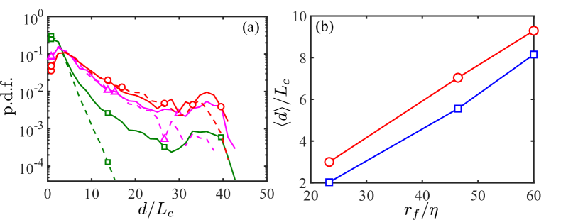
Figure 5: (a) P.d.f. of the diagonal length of individual three-dimensional $\varPi$ structures for $r_{f}=23.3\eta$ ($\square$), $r_{f}=46\eta$ ($\triangle$), and $r_{f}=60\eta$ ($\bigcirc$). Solid and dashed lines are for $\varPi^{+}$ and $\varPi^{-}$, respectively. (b) Mean value of the diagonal length of individual three-dimensional $\varPi$ structures as a function of the filter width. Colours and symbols are red circles for $\varPi^{+}$ and blue squares for $\varPi^{-}$.

3.2 Coherent flow associated with the energy cascades

Once we have established the self-similar organisation of the cascades in space, we characterise the three-dimensional flow conditioned to the presence of $\varPi$-structures. We follow the methodology of Dong et al. (2017); i.e., the flow is averaged in a rectangular domain whose centre coincides with the centre of gravity of the $n$-th structure, $\boldsymbol{x}_{c}^{n}$, and its edges are $\boldsymbol{r}=(r_{x},r_{y},r_{z})$ times the diagonal length $d^{n}$ of the bounding box of the structure. The conditionally averaged quantity $\widetilde{\phi}$ is then computed as

$$\{\widetilde{\phi}\}(\boldsymbol{r})=\sum_{n=1}^{N}\frac{\widetilde{\phi}(\boldsymbol{x}_{c}^{n}+d^{n}\boldsymbol{r})}{N},$$ (14)

where $n=1,..,N$ is the set of $\varPi$-structures selected for the conditional average. In the remainder of this work, the results are for $r_{f}=60\eta$, but similar conclusions are drawn for $r_{f}=23.3\eta$ and $r_{f}=46.6\eta$. Additionally, we focus on the energy-transfer mechanism for $\varPi$-structures with sizes larger than the Corrsin length-scale, $d>L_{c}$, above which the mean shear dominates.

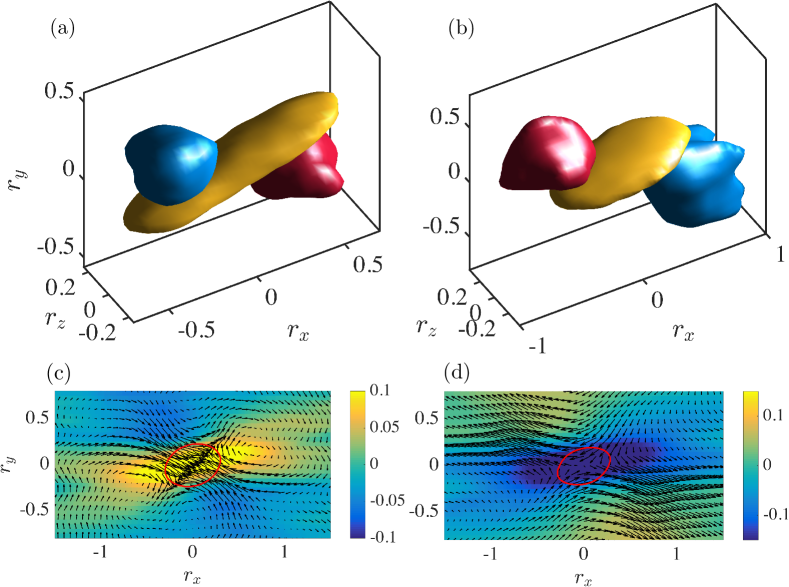
Figure 6: Averaged flow fields conditioned on $\varPi^{+}$-structures (a,c), and $\varPi^{-}$-structures (b,d). The isosurfaces in (a) and (b) are regions where $-\{\widetilde{u}\}\cdot\{\widetilde{v}\}$ and $\{\partial_{y}{\widetilde{u}}\}$ are larger than 0.4 and 0.7 of their maximum values in the domain, respectively. The colours are blue for the sweep, red for the ejection, and yellow for the shear layer. In panels (c) and (d), the arrows are $(\{\widetilde{u}\},\{\widetilde{v}\})$, and the colours represent $\{\partial_{y}{\widetilde{u}}\}$. Velocities are normalised by $SL_{z}$, $\partial\widetilde{u}/\partial y$ is normalised by the mean shear rate $S$, and distances are normalised by the diagonal length of individual structures as seen in (14). The solid red lines in panels (c) and (d) represent 0.6 of the maximum probability of finding a point belonging to a $\varPi^{+}$ or $\varPi^{-}$ structure, respectively.

3.2.1 Averaged flow field conditioned on intense $\varPi$

The three-dimensional velocities conditioned on intense structures of $\varPi^{+}$ and $\varPi^{-}$ are disclosed in figure 6(a,c) and (b,d), respectively. Panels (a) and (b) show the averaged tangential Reynolds stress $\{\widetilde{u}\}\cdot\{\widetilde{v}\}$ and shear layer $\{\partial_{y}{\widetilde{u}}\}$. To facilitate the visualisation of the velocity field, figures 6(c) and (d) contain the vector field $(\{\widetilde{u}\},\{\widetilde{v}\})$ overlaid with $\{\partial_{y}{\widetilde{u}}\}$ in the plane $r_{z}=0$. Regions of intense $\varPi$ are closely associated with a sweep ($\{\widetilde{u}\}>$0, $\{\widetilde{v}\}<$0) and an ejection ($\{\widetilde{u}\}<$0, $\{\widetilde{v}\}>$0) represented by the regions coloured in blue and red, respectively, in figures 6(a) and (b). For the forward cascade, the ejection is located downstream and beneath $\varPi^{+}$, while the sweep occurs upstream and above $\varPi^{+}$. Conversely, the positions of the sweep and the ejection are interchanged for intense $\varPi^{-}$.

Interestingly, figure 6(c) shows that the forward energy transfer is confined within a large-scale shear layer (the yellow region in figure 6a) originated by the collision of the sweep and the ejection. Inversely, as shown in figure 6(d) the backward energy transfer occurs within the saddle region induced by the separation of the sweep and the ejection. The shear layers are inclined with respect to the streamwise direction by roughly $16^{\circ}$, with a characteristic length of about two times the diagonal length of the associated $\varPi$ structure. The inclination angle is almost identical to that of the streamwise fluxes train shown in figure 4(b). The intensity of the shear layer around $\varPi$ is 10% of $S$ owing to the lack of small scales motions, which are filtered out. The intensities of the averaged vertical velocity $\{\widetilde{v}\}$ conditioned on $\varPi^{+}$ and $\varPi^{-}$ are almost identical, but the averaged streamwise velocity $\{\widetilde{u}\}$ conditioned on $\varPi^{-}$ is roughly twice of that conditioned on $\varPi^{+}$.

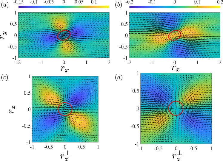
Figure 7: The averaged vorticity field conditioned on intense $\varPi^{+}$ (a,c) and $\varPi^{-}$ (b,d). Panels (a) and (b) are for spanwise vorticity $\{\widetilde{\omega_{z}}\}$ in the same plane as figure 6(a,b). Panels (c-d) are for $(\{\widetilde{\omega_{x}}\}$+$\{\widetilde{\omega_{y}}\})$cos$(45^{\circ})$ in the plane containing $\boldsymbol{\delta}=\textbf{0}$ with an inclination angle 135^∘ with respect to the streamwise direction. $\delta_{z}^{\bot}=\delta_{y}/$cos$(45^{\circ})$. Arrows represent $(\{\widetilde{u}\},\{\widetilde{v}\})$ in (a-d) and $(\{\widetilde{w}\}^{\bot},\{\widetilde{w}\})$ in (c,d), where $\{\widetilde{w}\}^{\bot}=(\{\widetilde{v}\}-\{\widetilde{u}\})$cos$(45^{\circ})$. The range of the contour is $[-0.25\ 0.25]S$ in (a-b) and $[-0.125\ 0.125]S$ in (c-f) from blue to yellow. The solid red lines are the same as in figure 6

The velocity patterns shown in figure 6, as well as the inclination angle of the shear layer, agree well with those in zero-pressure-gradient turbulent boundary layer (Natrajan & Christensen, 2006), in the channel with rough walls (Hong et al., 2012) and in the atmosphere boundary layer with near-neutral atmospheric stability (Carper & Porté-Agel, 2004). However, the organisation of the ejection and the sweep in SS-HST around $\varPi$ is symmetric due the nature of the flow, in contrast to the pattern observed in the near-wall region of wall-bounded turbulence (Piomelli et al., 1996; Carper & Porté-Agel, 2004).

We analyse next the organisation of the vorticity $\{\widetilde{\omega_{i}}\}$ around intense energy transfer events. To gain a better insight into the flow organisation, it is convenient to represent the flow in the plane aligned with the mean inclination angle of the shear layer. Figure 7(c-d) shows ($\{\widetilde{\omega_{x}}\}$+$\{\widetilde{\omega_{y}}\}$)cos$(45^{\circ})$ in the plane ($z^{\bot}-z$), which is inclined by 135^∘ with respect to the streamwise direction. The ($z^{\bot}-z$) plane contains $\boldsymbol{\delta}=\textbf{0}$ and cuts through the centre of $\{\widetilde{\omega_{x}}\}$ and $\{\widetilde{\omega_{y}}\}$, with $z^{\bot}$ defined by $y/\textup{cos}(45^{\circ})$. The velocity vectors in figure 7(c-d) are $(\{\widetilde{w}\}^{\bot},\{\widetilde{w}\})$ with $\{\widetilde{w}\}^{\bot}=(\{\widetilde{v}\}-\{\widetilde{u}\})$cos$(45^{\circ})$. The inclination angles of the vorticity pairs with the same sign in $z^{\bot}-z$ plane are also $45^{\circ}$ or $135^{\circ}$.

Figure 7(a-b) show the conditional averaged spanwise vorticity, $\{\widetilde{\omega_{z}}\}$, in the same plane as in figure 6(c-d). The average spanwise vorticity shows a quadrupolar configuration: one pair of $\{\widetilde{\omega_{z}}\}$ is inclined by the same angle as the shear layer, whereas a weaker second pair appears with opposite sign normal to the shear layer. The result differs slightly from the observations in the channel flows with rough walls (Hong et al., 2012), where the $\{\widetilde{\omega_{z}}\}$ inclined with the shear layer does not form a pair, but a train in the downstream of the flux. The conditional averaged $\{\widetilde{\omega_{x}}\}$ and $\{\widetilde{\omega_{y}}\}$ also adopt a quadrupolar configuration, but different from the one obtained for $\{\widetilde{\omega_{z}}\}$. Both $\{\widetilde{\omega_{x}}\}$ and $\{\widetilde{\omega_{y}}\}$ are parallel to the $x-y$ plane and are inclined by $45^{\circ}$ with respect to the streamwise direction.

The quadrupolar $\{\widetilde{\omega_{y}}\}$ was also observed in the inner mixing zone of flow induced by the Richtmyer-Meshkov instability at the early stage of mixing process (Liu & Xiao, 2016), in the zero-pressure-gradient turbulent boundary layer (Carper & Porté-Agel, 2004) and in the channel with rough walls (Hong et al., 2012). In the latter two cases, the counter rotating $\{\widetilde{\omega_{y}}\}$ pairs in the downstream and upstream of the flux have different intensities, which reflects the different intensities of sweeps and ejections.

In summary, the flow patterns reported above suggest that the flow around $\varPi^{+}$ forms a saddle region contained in the streamwise and vertical direction such that $\{\partial_{x}\widetilde{u}\}<0$, $\{\partial_{y}\widetilde{v}\}<0$ and $\{\partial_{z}\widetilde{w}\}>0$. The reversed pattern is observed for the flow around $\varPi^{-}$. Such abrupt changes would cause strong gradients and a significant kinetic energy transfer. The decomposition of $\varPi$ as the sum $\varPi=\sum_{ij}\varPi_{ij}$ with $\varPi_{ij}=-\tau_{ij}\partial\tilde{u}_{i}/\partial x_{j}$ reveals that, $\varPi_{11}$, $\varPi_{33}$ and $\varPi_{12}$ are the dominant terms, contributing 61.5%, $-$30.0% and 48.8%, respectively, to the total $\varPi$.

3.2.2 Connection between conditional flow fields, vortex stretching, and strain self-amplification

A vast body of literature places vortex stretching at the core of the energy transfer mechanism among scales (Leung et al., 2012; Goto et al., 2017; Lozano-Durán et al., 2016; Motoori & Goto, 2019), while recent works suggest that strain-rate self-amplification is the main contributor to the energy transfer (Carbone & Bragg, 2019). Thus, it is relevant to explore the connection between the flow structure identified in §3.2.1 and the vortex stretching and strain self-amplification mechanisms. Following Betchov (1956), the vortex stretching rate can be expressed as

$$\widetilde{\boldsymbol{\omega}}^{\top}\widetilde{\boldsymbol{S}}\widetilde{\boldsymbol{\omega}}=-4\textup{Tr}(\widetilde{\boldsymbol{S}}^{3})=-12\alpha\beta\gamma,$$ (15)

where $\widetilde{\boldsymbol{S}}$ is the filtered rate of strain tensor, and $\alpha\geq\beta\geq\gamma$ are its real eigenvalues. The incompressibility condition requires that $\alpha+\beta+\gamma=0$. The largest eigenvalue $\alpha$ is always positive (extensional), $\gamma$ is always negative (compressive), while $\beta$ can be either positive or negative depending on the magnitudes of $\alpha$ and $\gamma$. Hence, the role played by vortex stretching is controlled by the sign of $\beta$. The values of $\beta$ conditioned on $\varPi^{+}$ and $\varPi^{-}$ are shown in figure 8. At the core of $\varPi^{+}$, $\beta>0$, which implies that, on average, $\widetilde{\boldsymbol{\omega}}^{\top}\widetilde{\boldsymbol{S}}\widetilde{\boldsymbol{\omega}}>0$. The opposite is true at the core of $\varPi^{-}$, where $\widetilde{\boldsymbol{\omega}}^{\top}\widetilde{\boldsymbol{S}}\widetilde{\boldsymbol{\omega}}<0$ in the mean. The previous outcome suggests that vortex stretching is active during the forward cascade, while the vortex destruction dominates in regions of backward cascade. Similarly, the strain self-amplification rate is

$$\widetilde{\boldsymbol{S}}^{\top}\widetilde{\boldsymbol{S}}\widetilde{\boldsymbol{S}}=-\frac{3}{4}\widetilde{\boldsymbol{\omega}}^{\top}\widetilde{\boldsymbol{S}}\widetilde{\boldsymbol{\omega}},$$ (16)

and the strain destruction ($\boldsymbol{S}^{\top}\boldsymbol{S}\boldsymbol{S}<0$) is bound to dominate in the regions of forward cascade, whereas the strain amplification ($\boldsymbol{S}^{\top}\boldsymbol{S}\boldsymbol{S}>0$) is active within backward cascade events.

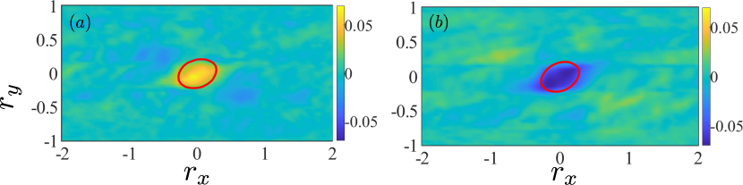
Figure 8: The averaged $\beta$ (intermediate eigenvalue of $\boldsymbol{S}$) conditioned on intense $\varPi^{+}$ (a) and $\varPi^{-}$ (b). The values of $\beta$ are normalised by the mean shear $S$.

3.2.3 Relation between intense $\varPi$ and hairpins

We inspect the enstrophy structure surrounding the forward and backward energy cascades. To this end, we compute the averaged enstrophy $\{\widetilde{\omega}\}^{2}=\{\widetilde{\omega_{x}}\}^{2}+\{\widetilde{\omega_{y}}\}^{2}+\{\widetilde{\omega_{z}}\}^{2}$ conditioned on structures of forward and backward kinetic energy transfer, where $\omega_{i}$ is the vorticity. As seen in figure 9, both $\varPi^{+}$ and $\varPi^{-}$ are located at the leading edge of an upstream inverted hairpin and at the trailing edge of a downstream upright hairpin. Given the average nature of the conditional flow, the emerging upright and inverted hairpins should be appraised as statistical manifestations rather than instantaneous features of the flow.

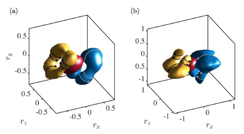
Figure 9: Averaged conditional enstrophy $\{\widetilde{\omega}\}^{2}=\{\widetilde{\omega_{x}}\}^{2}+\{\widetilde{\omega_{y}}\}^{2}+\{\widetilde{\omega_{z}}\}^{2}$ associated with forward (a) and backward (b) cascades. Upright and inverted hairpins, defined by $\{\widetilde{\omega}\}^{2}$=0.5$\{\widetilde{\omega}\}^{2}_{\textup{max}}$, are coloured in blue and yellow, respectively. The isosurface coloured in red is 0.7 of the maximum probability of finding a point belonging to a $\varPi$-structure. The curved arrows indicate the direction of rotation of the flow based on the signs of averaged vorticities. In particular, the rotation of the legs is based on the signs of the averaged $\omega_{x}$ and $\omega_{y}$, while the rotation at the head is based on the averaged $\omega_{z}$.

It was assessed that repeating the analysis using only half of the flow fields does not altered the conclusions presented above. More precisely, if we denote by $\{\tilde{\omega}\}_{1}$ and $\{\tilde{\omega}\}_{2}$ the average vorticity field obtained using all and half of the flow fields, respectively, the relative difference between both fields was found to be at most 1%. Similar values are obtained for other quantities.

Our results show that both upright and inverted hairpins are involved in the kinetic energy transfer. The flow representation promoted above differs from previous models in which upright hairpins dominate (Carper & Porté-Agel, 2004; Natrajan & Christensen, 2006). The sweep and ejection around the kinetic energy flux are attributed respectively to the head and legs of upright hairpins. Nonetheless, those studies were hampered by two-dimensional observations, whereas we have highlighted that a fully three-dimensional analysis is necessary to elucidate the actual enstrophy structure of $\varPi$. As supplementary material, we provide videos of the flow patterns in figure 9 and figures 6(a,b) to assist the reader in understanding the spatial structure of the energy cascade [movie_S1,S2,S3, and S4]. Individual inverted hairpins have been observed numerically and experimentally in homogeneous shear turbulence (Kim & Moin, 1987; Vanderwel & Tavoularis, 2011) and in channels flows (Kim & Moin, 1986), and other investigations have also linked $\varPi^{+}$ to U-shaped regions in the flow (Gerz et al., 1994; Finnigan et al., 2009; Hong et al., 2012) akin to the inverted hairpin reported here. Hong et al. (2012) concluded that both the sweep and the ejection around $\varPi^{+}$ are induced by the legs hairpins aligned in the streamwise direction. Our results suggest, however, that both upright and inverted hairpins are involved in the generation of sweeps and ejections around $\varPi$.

4 Conclusions

We have studied the three-dimensional flow structure and organisation of the kinetic energy transfer in shear turbulence for flow scales above the Corrsin length. Our analysis is focused on spatially intermittent regions where the transfer of energy among flow scales is intense. The structure of the velocity and enstrophy fields around these regions has been investigated separately for forward cascade events and backward cascade events.

The inspection of the relative distances between forward and backward cascades has shown that positive and negative energy transfers are paired in the spanwise direction and that such pairs form a train aligned in the mean-flow direction. Our results also indicate that the latter arrangement is self-similar across flow scales. We have further uncovered that the energy transfer is accompanied by nearby upright and inverted hairpins, and that the forward and backward cascades occur, respectively, within the shear layer and the saddle region lying in between the hairpins. The asymmetry between the forward and backward cascades emerges from the opposite flow circulation of the associated upright/inverted hairpins, which prompts reversed patterns in the flow. To date, the present findings represent the most detailed structural description of the energy cascade in shear turbulence. In virtue of the previously reported similarities between wall turbulence and SS-HST, we expect our results to be representative of wall-bounded flows. Nonetheless, additional efforts should be devoted to confirm this scenario in other flow configurations.

We have applied our method to the simplest shear turbulence, but nothing prevents its application to the inertial range of isotropic turbulence and to more complex configurations with rotation, heat transfer, electric fields, quantum effects, etc. Finally, the characterisation of the cascade presented in this study is static and do not contain dynamic information on how the kinetic energy is transferred in time between hairpins at different scales. Therefore, our work is just the starting point for future investigations and opens new venues for the analysis of the time-resolved structure of the energy cascade (Cardesa et al., 2017), including cause-effect interactions among energy-containing eddies (Lozano-Durán et al., 2020).