Identifying Exoplanets with Deep Learning III: Automated Triage and Vetting of TESS Candidates

Abstract

NASA’s Transiting Exoplanet Survey Satellite (TESS) presents us with an unprecedented volume of space-based photometric observations that must be analyzed in an efficient and unbiased manner. With at least $\sim 1,000,000$ new light curves generated every month from full frame images alone, automated planet candidate identification has become an attractive alternative to human vetting. Here we present a deep learning model capable of performing triage and vetting on TESS candidates. Our model is modified from an existing neural network designed to automatically classify Kepler candidates, and is the first neural network to be trained and tested on real TESS data. In triage mode, our model can distinguish transit-like signals (planet candidates and eclipsing binaries) from stellar variability and instrumental noise with an average precision (the weighted mean of precisions over all classification thresholds) of 97.0% and an accuracy of 97.4%. In vetting mode, the model is trained to identify only planet candidates with the help of newly added scientific domain knowledge, and achieves an average precision of 69.3% and an accuracy of 97.8%. We apply our model on new data from Sector 6, and present 288 new signals that received the highest scores in triage and vetting and were also identified as planet candidates by human vetters. We also provide a homogeneously classified set of TESS candidates suitable for future training.

.pspdf.pdfps2pdf -dEPSCrop -dNOSAFER #1

1. Introduction

The advent of large-scale transit surveys revolutionized our understanding of exoplanets. Both ground-based and space-based telescopes, such as OGLE (Udalski et al., 2002), TrES (Alonso et al., 2004), HATNET/HATS (Bakos et al., 2004), WASP (Pollacco et al., 2006), KELT (Siverd et al., 2009), and CoRoT (Auvergne et al., 2009), have provided us with an unprecedented volume and rate of new discoveries. Perhaps the most notable of all these surveys is NASA’s Kepler space telescope (Borucki et al., 2010; Koch et al., 2010). Over the course of its four-year mission, Kepler observed a total of 200,000 stars, including hosts of more than 2,000 confirmed planets (Borucki, 2016). After the failure of two of its reaction wheels, the repurposed spacecraft (K2; Howell et al., 2014) yielded another $\sim 360$ confirmed planets across the ecliptic plane (e.g. Crossfield et al., 2016; Mayo et al., 2018; Livingston et al., 2018a, b). Kepler’s successor, the recently launched Transiting Exoplanet Survey Satellite (TESS; Ricker et al., 2014) will likely more than double the number of known exoplanets (Sullivan et al., 2015; Huang et al., 2018a). During its two-year mission duration, TESS will observe the sky in $24^{\circ}\times 96^{\circ}$ sectors and downlink data twice during every 27-day sector, eventually covering 20 million stars and 90% of the sky (Sullivan et al., 2015). Because TESS observes in the anti-Sun direction (Ricker et al., 2014), TESS targets can be immediately observed from the ground if identified sufficiently rapidly. Prompt follow-up observations are rendered even more crucial by TESS’s shorter observing windows, which mean that ephemeris decay (increasing uncertainty in future transit times as we extrapolate our predictions beyond the data used to determine the ephemeris) presents a much bigger problem for TESS than for Kepler and K2 (Dragomir et al. in prep.).

Despite the need for rapid and accurate planet candidate identification, space surveys like TESS continue to rely on human vetting. Typically, teams of experts manually examine possible planet signals and vote on their final dispositions (e.g. Yu et al., 2018; Crossfield et al., 2018, Guerrero et al. in prep). This process can be quite time-consuming: for a typical TESS sector, it may take a few experienced humans up to a few days to perform triage, i.e. the procedure of rapidly eliminating the obvious false positives, on tens of thousands of candidates. Then, a team of $\sim 10$ vetters may spend up to a week classifying the remaining $\sim 1,000$ high-quality candidates if we require each one to be viewed by at least three different people. Furthermore, human vetters may not always maintain a consistent set of criteria when judging potential planetary signals. Even an experienced team of vetters may sometimes disagree on the disposition of a TCE, and dispositions given to the same object may vary depending on, for example, the manner of presentation, other TCEs viewed recently, or even the time of day, as we have seen both in Kepler vetting (e.g. Coughlin et al., 2016) and in our own experience with TESS.

In response to these shortcomings in human vetting, a number of efforts have emerged to classify light curves automatically and uniformly. Non-machine learning methods make use of classical tree diagrams with criteria designed to mimic the manual process for rejecting false positives (Coughlin et al., 2016; Mullally et al., 2016). These were completely automated by the end of the Kepler mission. Early works on using machine learning to classify Kepler light curves have explored techniques such as $k$-nearest neighbors (Thompson et al., 2015), random forests (McCauliff et al., 2015; Mislis et al., 2016), and self-organizing maps (Armstrong et al., 2017). Convolutional neural networks (CNNs), a class of deep neural networks that has proven successful in image recognition and classification, emerged as another possible method. Zucker & Giryes (2018) and Pearson et al. (2018) investigated the feasibility of using CNNs to detect transiting planets by applying them to simulated data. The first successful CNN that identified planets in real data from Kepler was AstroNet (Shallue & Vanderburg, 2018). Ansdell et al. (2018) further improved upon the model by incorporating scientific domain knowledge. Since then, researchers have either modified the original AstroNet model or created their own CNNs to classify candidates from ground-based surveys (Schanche et al., 2019) and K2 (Dattilo et al., 2019). Osborn et al. (2019) registered the first attempt to adapt AstroNet for TESS candidates, but the model was trained on simulated data, which are likely to have very different systematics from real TESS data. As a result, the model suffers a deterioration in performance when applied to real TESS data, recovering about 61% of the previously identified TESS objects of interest.

Here we present the first CNN trained and tested on real TESS data. Our model takes as inputs human-labeled light curves produced by the MIT Quick Look Pipeline (Huang et al. in prep.), and can be trained to perform either triage or vetting on TESS candidates. This paper is organized as follows: In Section 2, we describe the creation of the data set used in this study, including how we produced and labeled the light curves; Section 3 describes the architecture and training of our neural network for triage and vetting purposes; in Section 4, we evaluate the ability of our neural network to identify planet-like events in the test set; in Section 5, we apply our neural network to new data from TESS Sector 6 and present a number of new planet candidates; finally, we discuss some potential improvements to our model in Sector 6. All of our code and the list of labeled TESS targets used in this paper are publicly available.

2. Data set

Since our goal is to create a neural network capable of performing triage and vetting on TESS light curves, we train and test our models using TESS light curves from Sectors 1-5. Here, we give a brief overview of how these light curves are produced and processed prior to training. We also describe some additional criteria we use to refine this data set.

2.1. Identifying Threshold-Crossing Events

Like Shallue & Vanderburg (2018), we work with possible planet signals, which are called “threshold-crossing events” or TCEs. These are periodic dimming events potentially consistent with signals produced by transiting planets, and are typically identified by an algorithm designed to find such signals. In this study, we adopt the MIT Quick Look Pipeline (QLP; Huang et al. in prep) for light curve production and transit searches. The QLP is partially based on fitsh (Pál, 2009), and is designed to process TESS full-frame images (FFIs) that are obtained with 30-minute time sampling. Immediately upon data downlink, the QLP produces light curves using internal calibrated images from the MIT Payload Operation Center and identifies TCEs. It has already been used to find and alert planet candidates from early TESS sectors (e.g. Huang et al., 2018b; Vanderspek et al., 2019; Rodriguez et al., 2019).

2.1.1 Light Curve Production

The QLP uses a catalog-based circular aperture photometry method to extract light curves for all stars in the TESS Input Catalog (TIC) with TESS-band magnitudes brighter than 13.5. The apertures are centered based on a predetermined astrometric solution derived on each observed frame using stars with TESS magnitudes between 8-10. The light curves are extracted using five circular apertures. The background is estimated using annuli around the target star on difference images and a photometric reference frame. The photometric reference is computed using the median of 40 frames with minimal scattered light. The difference images are computed using a direct subtraction of the photometric reference frame from the observed frames.

The light curves produced this way usually contain low-frequency variability from stellar activity or instrumental noise. Following Vanderburg & Johnson (2014), the QLP removes this variability by fitting a B-spline to the light curve and dividing the light curve by the best-fit spline. Outlier points caused by momentum dumps or other instrumental anomalies are masked out prior to detrending. To avoid distorting any transits present, we iteratively fit the spline, remove $3\sigma$ outliers, and refit the spline while interpolating over these outliers (see Fig. 3 in Vanderburg & Johnson, 2014). We then select an optimal aperture for stars in each magnitude range (13 linear bins between TESS magnitudes of 6-13.5) by determining which aperture size produces the smallest photometric scatter in the magnitude bins.

The light curves are extracted and detrended one TESS orbit at a time, and then stitched together into multi-sector light curves after dividing out the median levels of the detrended light curves. By Sector 6, stars observed in TESS’s continuous viewing zone have light curves with baselines of $\approx$ 166 days, while stars observed in camera 1 (closest to the ecliptic plane) have baselines of only a single $\approx$ 27 day TESS sector.

2.1.2 Transit Search

After producing a detrended light curve for each star using its optimal aperture, the QLP searches the light curves for periodic dipping signals using the Box Least Squares algorithm (BLS; Kovács et al., 2002). We perform the search for periods ranging from $0.1$ days, to half the length of the longest baseline expected for the given camera. The number and spacing of frequencies searched by BLS is adapted to the total baseline in the light curves as well, following Vanderburg et al. (2016). We designate any signal with a signal-to-pink-noise ratio (SNR, as defined by Hartman & Bakos, 2016) $>9$ and BLS peak significance $>10$ as a TCE. The BLS peak significance is defined as the height of the BLS peak in the spectrum compared to the noise floor of the BLS spectrum.

2.2. “Ground Truth” Labels

Unlike the Kepler DR24 data set used by Shallue & Vanderburg (2018), our TESS TCEs do not come with a complete set of human-assigned labels. A small fraction of TCEs underwent group vetting, in which a team of human vetters closely examined the signals using candidate reports created by the QLP and voted on their dispositions, but even this process can yield inconsistent results: a TCE that appears in more than one sector can have different dispositions in different sectors. To ensure homogeneity in the labeling, one of us (LY) visually inspected the light curves of all the TCEs and assigned each to one of four categories: planet candidates (PC), eclipsing binaries (EB), stellar variability (V) and instrumental noise (IS). We used the following set of rules to guide our classification:

• Any planet-like signal that does not have a strong secondary eclipse, odd/even transit shape differences, or transit depths that increase with aperture size (indicating that the source of the transit is off-target) is classified as PC.

• Some transiting brown dwarfs and M dwarfs have previously been identified as eclipsing binaries in ground-based surveys (e.g. Triaud et al., 2017; Collins et al., 2018) and assigned EB labels in group vetting, but without information beyond the TESS data, even experienced human vetters cannot distinguish these systems from transiting giant planets. We relabel these TCEs as PCs in the data set.

• Our data set contains one known planet with visible secondary eclipses, namely the hot Jupiter WASP-18b (Hellier et al., 2009; Shporer et al., 2019). We assigned this planet to the PC class.

• Off-target transit signals whose depths increase with aperture size are always labeled as EBs, regardless of whether the signals could be consistent with planetary transits after correcting for dilution.

• Some eclipsing binary systems also exhibit stellar variability. We classify such systems as V if the amplitude of the variability is more than half the eclipse depth, and as EB otherwise.

• Any TCEs that are so ambiguous that even human vetters cannot decide whether they are viable planet candidates or false positives are removed from the training set.

• PCs and EBs that are significantly distorted by detrending (i.e. if the transits are no longer recognizable as transits, or if their depths change by 50% or more) are removed from the training set.

• We do not make any cuts on transit depth. Deep transit signals that do not show any other signs of being eclipsing binaries are still classified as PCs. The deepest transit in our data set has a depth of 8%.

• Unusual signals that do not fit well into any of the four categories are classified as V.

For the rest of the paper, we assume that these dispositions are the ground truth, even though they may not be perfect. It is likely that a small number of TCEs are misclassified, especially ones that exhibit both stellar variability and eclipses. There may also be a few duplicates in the data set. But since the number of such errors is very small, we expect their impact on our model and performance metrics to be minimal. There are also cases where BLS misidentified the period of a TCE. We corrected as many of these as possible by hand. Occasionally, BLS identifies single-transit events at a fraction of the true period. Our dataset included 20 such singly-transiting EBs and 9 singly-transiting PCs. We do not know the exact periods of these objects, so we use the smallest integer multiple of the BLS period that exceeds the baseline as a guess for the true period. Since the duty cycle of the transit provides information on the density of the host star, which may be useful in distinguishing PCs from EBs (large duty cycles typically indicate that the host star is a giant, and therefore more likely to host EBs), any inaccurate estimates of the period would only be a potential concern in vetting, not in triage. But the number of PCs affected is also small, so again we do not expect them to have a large impact on our model’s performance.

After manually assigning labels to all TCEs, we binarize the labels as “planet-like” and “non planet-like”. When using our neural network to perform triage, both the PC and EB classes are considered to be “planet-like”, so that we retain as many potential planet candidates as possible. When using the network for vetting, we perform a more rigorous selection and only consider PCs as “planet-like”.

We make use of TCEs from TESS Sectors 1-4, but because the V and IS classes drastically outnumber both PCs and EBs, we supplemented our data set with 296 PCs and EBs from Sector 5. In total, we have 16,516 TCEs for triage, including 493 PCs, 2,155 EBs and 13,868 V and IS combined. If an object is identified as a TCE in multiple sectors, we break up the light curve into individual sectors and count each sector as a separate object. For vetting, another 65 TCEs were discarded due to an insufficient number of points ($<$ 5) to construct secondary eclipse views, resulting in 492 PCs, 2,154 EBs and 13,805 V and IS combined. We randomly shuffle and partition them into three subsets: training (80%), validation (10%) and test (10%). The validation set is used to choose model hyperparameters during training, and the test set to evaluate final model performance.

2.3. Preparing Input Representations

Following Shallue & Vanderburg (2018), we process each light curve into a standardized input representation before feeding it into the neural network. Since the QLP already removes low-frequency variability from the light curves, we skip the detrending step. The light curve is then phase-folded at the period identified by BLS, such that the transits are lined up and centered. We remove any points corresponding to images with non-zero data quality flags, and any upward outliers that are more than 5 times the median absolute deviation away from the median.

We then binned the data into two views, similar to those described in Shallue & Vanderburg (2018): a “global view”, which shows the light curve over an entire orbital period; and a “local view”, which is a close-up of the transit event, spanning no more than two transit durations on either side of the transit mid-point. Shallue & Vanderburg (2018) grouped their phase-folded light curves into 2,001 bins for the global view, and 201 bins for the local view. The Kepler light curves used by Shallue & Vanderburg (2018) span up to 4 years in duration and contain approximately 70,000 points each. Many TESS light curves, on the other hand, only span about 27 days and have far fewer data points. The resulting phase-folded light curves are therefore much sparser than those from Kepler. For this reason, we reduced the number of bins in the global and local views to 201 and 61 respectively, and linearly interpolated the data over empty bins.

In vetting mode, we also prepare a “secondary eclipse view”, which was not present in the original AstroNet model, but was suggested as a possible improvement to the model by Shallue & Vanderburg (2018). We first perform a search for the most likely secondary eclipse by masking the transits in the phase-folded light curves and using a BLS-like algorithm to fit a box (whose width is fixed to that of the primary transit) to various positions between orbital phases 0.1 and 0.9 in the masked and folded light curve. The position that yields the highest S/N is assumed to be the midpoint of the most likely secondary eclipse. We then normalize and bin the folded light curve within up to two transit durations on either side of this location into 61 bins, following the exact same procedure we use to produce the local views.

Fig. 1 shows examples of global, local and secondary eclipse views for different classes of signals.

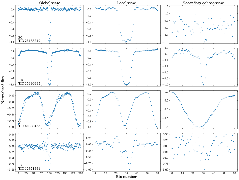
Figure 1.— For each TCE, we prepare three phase-folded, depth-normalized representations of the light curve: the “global view” (left column) is a fixed-length representation of the entire period; the “local view” (middle column) is a close-up view of the putative transit; the “secondary eclipse view” (right column), only present in vetting mode, is a close-up view of the most likely secondary eclipse. Each row presents an example from one of the four categories of TCEs: PC (planet candidates), EB (eclipsing binaries), V (stellar variability) and IS (instrumental artifact).

3. Neural Network

3.1. Architecture

Our neural network architecture is based on AstroNet, a deep convolutional neural network (CNN) developed by Shallue & Vanderburg (2018). CNNs are a class of deep learning model used for inputs with spatial structure (e.g. images or time series). A CNN contains a hierarchy of “convolutional layers.” Each convolutional layer performs a cross-correlation operation by sliding a small filter over the input, summing the result, and adding it to a feature map. Each filter activates in response to a specific feature or pattern in its input. A CNN typically contains many consecutive convolutional layers. In the deeper layers, simpler features learned in previous layers are combined into more complex features. During training, the parameters of the convolutional filters are adjusted to minimize a cost function, a measure of how far the model’s predictions are from the true labels in its training set.

AstroNet is implemented in TensorFlow (Abadi et al., 2016), an open source machine learning framework developed at Google Brain. The global and local view vectors (and secondary eclipse view in vetting mode) are passed through disjoint convolutional columns with max pooling, and then combined in shared fully connected layers ending in a sigmoid activation function. The model outputs a value in $(0,1)$, with values close to 1 indicating high confidence that the input is a transiting planet and values close to 0 indicating high confidence that the input is a false positive. Shallue & Vanderburg (2018) trained 10 independent copies of the model with different random parameter initializations and averaged the outputs from these 10 copies for all predictions. This technique, known as “model averaging”, improves the robustness of the predictions by averaging over the stochastic differences between the individual models. We refer the interested reader to the Shallue & Vanderburg (2018) paper for a more detailed description of convolutional neural networks and the associated terminology.

We have made a few key modifications to the original AstroNet architecture, depending on whether the model is used for triage or vetting. Here we describe the two different modes in detail.

3.1.1 Triage Mode

The main goal of triage is to eliminate all the obvious non-planetary signals among the TCEs. Most TCEs are caused by instrumental artifacts and stellar variability. The remaining TCEs (usually a mix of planet candidates, eclipsing binaries and blended eclipsing binaries) are then passed on to the vetting stage, where they are examined in more detail. Typically, triage is performed by a human who visually inspects the light curve of each TCE and separates the signals that do not look remotely planet-like at first glance. There are usually a large number of TCEs to be triaged (a few thousand per TESS sector). Our neural network’s triage mode, which we dub AstroNet-Triage, is designed to automate the triage process.

AstroNet-Triage serves to classify TCEs into “planet-like” (including PCs and EBs) and everything else. We find that the original AstroNet architecture works well for triage purposes, and that changing the architecture does not yield any significant improvement over the original model, so we make no modifications to the architecture in triage mode. We pass both the global and local views, described in Section 2.3, through separate convolutional columns before concatenating them in the fully connected layers. We reproduce this architecture in Fig. 2.

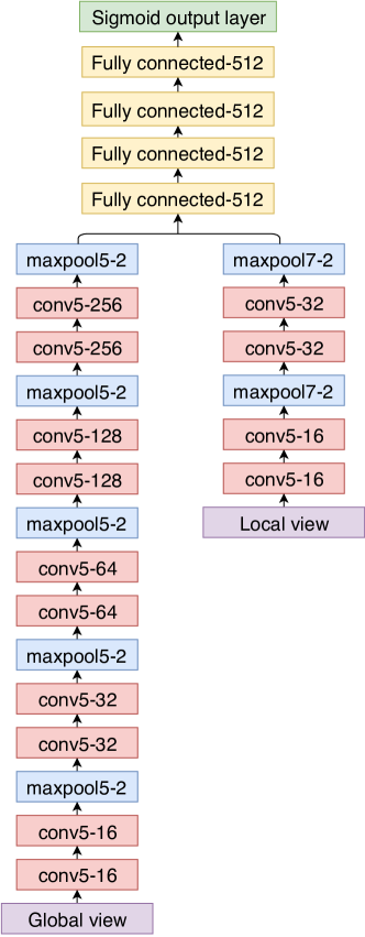
Figure 2.— The architecture of AstroNet-Triage (identical to that of the best-performing neural network from Shallue & Vanderburg, 2018). Convolutional layers are denoted conv$<$kernel size$>$-$<$number of feature maps$>$, maxpooling layers are denoted maxpool$<$window length$>$-$<$stride length$>$, and fully connected layers are denoted Fully connected-$<$number of units$>$.

3.1.2 Vetting Mode

When used for vetting, the model (dubbed AstroNet-Vetting) must also be able to distinguish EBs from PCs. Here we feed the global and local views to the neural network as we do in triage mode, but we also include a close-up of the most likely secondary eclipse (described in Section 2.3) in a disjoint convolutional column. In addition, we also concatenate a scalar feature to the outputs of the convolutional columns, namely the difference in transit depths measured in two apertures with radii of 2.75 and 3 pixels, divided by the out-of-transit standard deviation measured in the smaller aperture. We chose these two apertures because we find that they are generally large enough to encompass most of the flux from the target star, yet small enough to not include too much flux from background stars. The transit depths are estimated by fitting a box-shaped model to the light curves. This “depth change” feature is normalized by subtracting the mean of the entire training set and dividing by the standard deviation. The motivation behind adding a transit depth difference between different apertures is to help the model identify potential blends. When the source of a transit is off-target, a larger aperture typically produces a deeper transit than a smaller one. Transit depth differences are a simpler alternative to including the entire centroid time series, which Ansdell et al. (2018) and Osborn et al. (2019) used in their model. Also unlike Ansdell et al. (2018) and Osborn et al. (2019), we chose not to incorporate stellar parameters because a substantial fraction of our TCEs simply do not have stellar parameters available. This is because we search all stars in the FFIs, not just those selected for 2-minute-cadence observations. We also experimented with adding the TESS magnitude as a scalar feature, but its effect on the output is negligible. The architecture of the AstroNet-Vetting model is illustrated in Fig. 3.

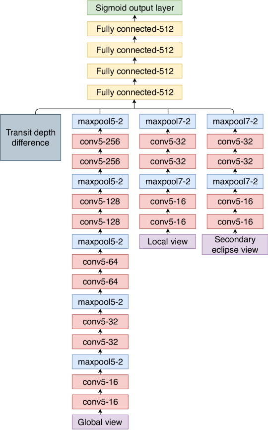
Figure 3.— Same as Fig. 2, but for AstroNet-Vetting.

3.2. Training

We trained the model for 14,000 steps on the training set in both the triage and vetting modes. We used the Adam optimization algorithm (Kingma & Ba, 2014) to minimize the cross-entropy error function over the training set. The number of training steps was chosen to minimize this error function over the validation set. During training, we augmented our training data by applying random horizontal reflections to the light curves with a 50% probability. This process generates similar but not identical samples with the same labels as the originals, thereby increasing the effective size of our training set and reducing the risk of overfitting. We trained the model with a batch size of 64, a learning rate of $\alpha=10^{-5}$, and exponential decay rates of $\beta_{1}=0.9$, $\beta_{2}=0.999$ and $\epsilon=10^{-8}$ (for more details on these parameters, see Kingma & Ba, 2014).

Like Shallue & Vanderburg (2018), we also make use of “model averaging” to improve the robustness of our predictions. We trained 10 independent, randomly initialized copies of the same model and used the average outputs of all copies for all predictions. Each copy may perform better or worse in different regions of parameter space due to its random parameter initialization, but model averaging averages over these differences. It also minimizes the stochastic differences that exist between individual models, thus making different configurations more comparable.

4. Evaluation of Neural Network Performance

We assess the performance of our neural network using the test set, the 10% of TCEs that were randomly left out of the training/validation sets and were thus not used to tune the model or its hyperparameters. Given the highly imbalanced nature of our training set, accuracy - the fraction of TCEs that the model correctly classified - is not a very useful measure of the model’s performance, because we can achieve high accuracy simply by classifying everything as negative (not planet-like). The same can be said of the AUC (area under the receiver-operator characteristic curve, equivalent to the probability that a randomly selected positive is assigned a higher prediction than a randomly selected negative). We therefore make use of three additional metrics: precision (reliability), recall (completeness) and average precision. Precision is defined as the fraction of all objects classified as positives that are indeed true positives. Recall is defined as the fraction of all positives in the test set that were correctly classified as positives. There is a trade-off between precision and recall depending on the classification threshold (the score above which we consider an object to be a positive): increasing the threshold typically raises the precision while lowering the recall, and vice versa. Average precision is the weighted mean of precisions achieved at each threshold, with the increase in recall from the previous threshold used as the weight.

In Fig. 4, we show the precision-recall (PR) curves for triage and vetting on our test set. Each point on a curve corresponds to the precision and recall values for that model at a different choice of classification threshold. For AstroNet-Vetting, we also plot separate PR curves for the original AstroNet model architecture and models with the two new features added individually to show the impact of each on model performance. Table 1 shows the accuracies (calculated for a classification threshold of 0.5), AUC, and average precisions achieved by all of these models on the test set. As mentioned earlier, the models can achieve very high accuracy and AUC in vetting mode and yet still struggle to produce a reliable planet sample.

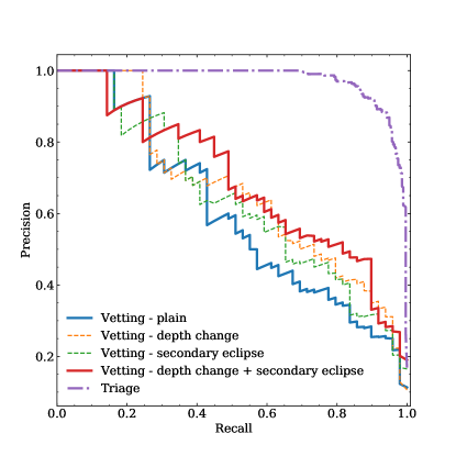
Figure 4.— Precision-recall curve of our neural network in both triage and vetting modes. The triage model is trained to distinguish PCs and EBs from obvious false positives, and the vetting model is trained to identify only PCs. The line labeled “vetting - plain” shows the original AstroNet model applied to vetting without the addition of any new features. The two dashed lines show the individual contributions of new features we added: “vetting - depth change” is the addition of transit depth differences alone, and “vetting - secondary eclipse” is the addition of secondary eclipse views. “Vetting - depth change + secondary eclipse” is the final AstroNet-Vetting model that combines both features.

Table 1Ensembled results achieved on the test set

Model	Accuracy	AUC	Average precision
Triage	0.974	0.992	0.970
Vetting - AstroNet plain	0.977	0.973	0.605
Vetting - depth change	0.978	0.980	0.669
Vetting - secondary eclipse	0.976	0.978	0.642
Vetting - depth change	0.978	0.984	0.693
+ secondary eclipse

We can also visualize the results in a different way. Fig. 5 shows a histogram of predictions given by the model to our test sets. The prediction loosely represents the probability that the model considers a given TCE to be a “positive”, meaning either a PC or EB in triage mode, or a PC in vetting mode. The color of each bar corresponds to the fraction of TCEs in that bin that are truly positives: a yellow bin contains mostly TCEs that are positives, while a blue bin contains mostly negatives. A good classifier would assign high predictions to positives and low predictions to negatives, so as to produce a histogram with yellow bins on the right side and blue bins on the left side. This is indeed what we see in both histograms.

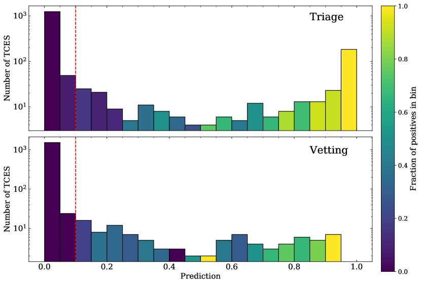
Figure 5.— Histogram of predictions on the test set by AstroNet-Triage (top) and AstroNet-Vetting (bottom). The color of each bar represents the fraction of TCEs in that bin that are actually positives (PCs and EBs in triage mode, and just PCs in vetting mode). A yellow bin contains mostly TCEs that are positives, while a blue bin contains mostly negatives. The red dashed line marks a classification threshold of 0.1, which we find to maximize the fraction of false positives eliminated while still retaining almost all of the PCs.

AstroNet-Triage is already capable of achieving high precision and recall. Since the primary goal of triage is to cull the list of candidates while preserving most or all true PCs, we choose a classification threshold of 0.1 in order to discard only TCEs that the model is confident are false positives. With this classification threshold, we reach a precision of 0.749 and a recall of 0.975 on our test set of 1,650 TCEs. We recover all of the 49 PCs and the vast majority of EBs, while still eliminating 93% of the negatives. The model can therefore be used to automatically eliminate obvious false positives in a set of TCEs with a minimal loss of PCs, allowing human vetters to focus instead on the strong candidate planets. The MIT TESS Team has already started using this model to perform triage on new TCEs from Sector 6 (see Section 5) and onward.

AstroNet-Vetting, on the other hand, is less successful and not ready to be used in production. A natural classification threshold for vetting would be 0.5, which would select only those TCEs that the model considers more-likely-than-not planets. However, we find that the vetting model has difficulty distinguishing some PCs from EBs: at a threshold of 0.5, we recover just 28 of the 49 PCs from the same test set with a precision of 0.651. Since TESS is a mission designed with follow-up in mind, we would rather retrieve as many PCs as possible at the expense of more false positives, which can be easily vetted out by follow-up programs. We therefore choose to evaluate our vetting model at the more conservative threshold of 0.1. At this threshold, we recover 44 of the 49 PCs with a precision of 0.449. Of the 5 missed PCs, three have systematics in their light curves that could have been mistaken for secondary eclipses, one is very V-shaped, and the last shows residual out-of-transit variability from imperfect detrending. 54 of the 69 false positives are EBs. A visual examination of the input representations of these misclassified EBs reveals that most do not have visible secondary eclipses nor exhibit significant changes in eclipse depth with aperture size. Most of these objects received EB labels during the initial inspection because they had odd-even transit differences or had synchronized out-of-transit variability that was later removed during detrending. These features are not captured in our input representation, so the model lacks sufficient information to distinguish these particular EBs from PCs. We discuss several ideas for improving the input representation in Section 6. The inability of the vetting model to separate EBs from PCs may also be due to the small number of PCs present in the training set. With the addition of new PCs from later TESS sectors, the model’s performance in vetting mode may continue to improve. Still, our current results and success in triage mode indicate that our approach to automated vetting is a promising one.

We note that even though AstroNet-Vetting cannot replace human vetting in its current state, and may never be able to do so completely, it can serve as a valuable complement to human vetting. This can help neutralize the shortcomings in both human and machine vetting. For example, it is difficult for human vetters to maintain a constant set of criteria when judging potential planet candidates, but machine learning can assign dispositions in a self-consistent, unbiased manner. On the other hand, a neural network can only detect patterns it was trained to detect. Unusual and interesting astrophysical signals that humans would recognize, such as WD 1145+017 b (Vanderburg et al., 2015) and KIC 8462852 (Boyajian et al., 2016), would likely be classified as IS or V and discarded by neural networks. It would be useful to compare lists of PCs produced by humans and neural networks.

5. Application to Previously Unseen TCEs

TESS finished observing Sector 6 on Jan 7, 2019. We directly applied the trained AstroNet-Triage model to 59,719 new TCEs with the strongest BLS signals from Sector 6. Among these, 11,895 TCEs received a triage score of 0.1 or higher. We manually examined a random subset of 3,177 TCEs with triage scores of 0.1 or higher, and TESS magnitudes brighter than 12. Among these, we labeled 2,223 as EBs, 415 as PCs and 539 as IS or V. So if we accept these manually assigned labels as the ground truth, the precision of our model is 0.83 at a threshold of 0.1. Therefore our model is able to successfully eliminate a large number of false positives from Sector 6 TCEs, despite being trained on previous sectors that may have different systematics. It is worth noting that Sector 6 also covers a different stellar population compared to Sectors 1-5: because of its proximity to the Galactic plane, there are more evolved and variable stars in Sector 6. That our model was able to attain a precision comparable to that from Sectors 1-5 indicates that the model generalizes well to previously unseen sectors. We are also starting to see similar systematics from sector to sector now, so once we have built up a large sample from data taken using the same pointing strategy, we may achieve an even better performance when extrapolating to future sectors.

Although AstroNet-Vetting is not quite ready to be used in production, we generated scores for the manually examined subset of 3,177 TCEs with AstroNet-Vetting as a demonstration of what we can achieve with purely automated vetting at this stage. 700 of these TCEs received vetting predictions of 0.1 or higher, including 288 of the 415 PCs. Fig. 6 shows 25 TCEs with the highest PC class probabilities that were also labeled as PCs by humans. At first glance, these do not show any warning signs of being non-planetary in nature (e.g. V-shaped transits or synchronized stellar activity). Our experience with Kepler, K2 and earlier TESS sectors leads us to believe that most of these are indeed planetary in nature, and can quickly be confirmed via follow-up observations. The transit properties from BLS for these TCEs and the remainder of the 273 highly ranked PCs are given in Table 2.

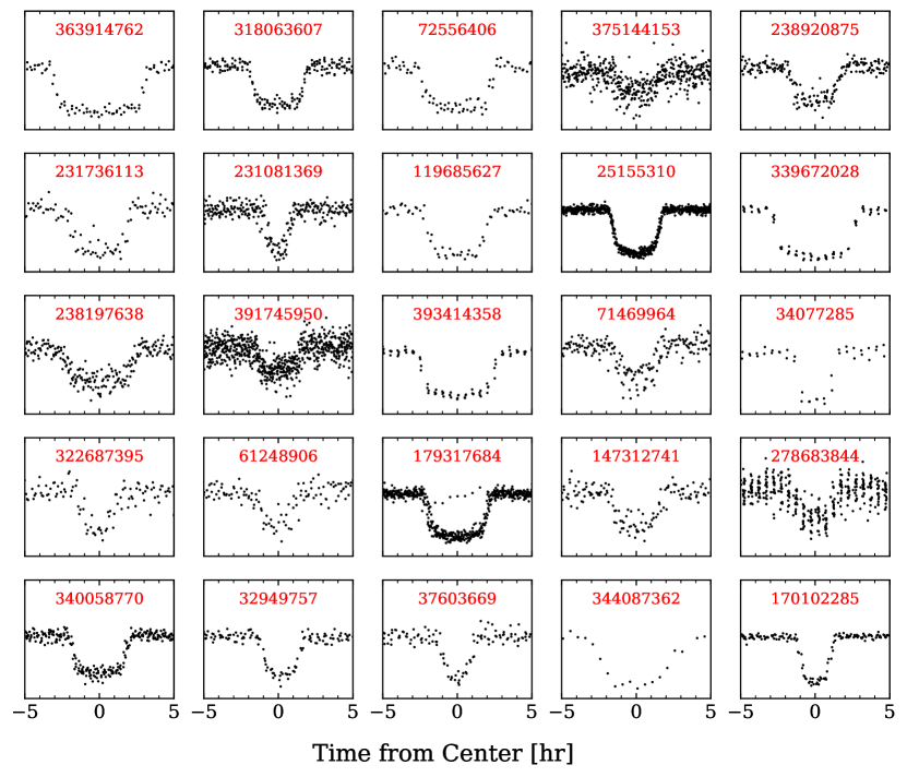
Figure 6.— Phase-folded light curves of our 25 highest-quality planet candidates from Sector 6, along with their TIC IDs. To avoid clutter, we did not label the y-axis. Their transit parameters are listed in Table 2.

6. Future Work

AstroNet-Triage is already quite successful at distinguishing “planet-like” TCEs (PCs and EBs) from instrumental noise and stellar variability, but both AstroNet-Triage and AstroNet-Vetting have room for improvement going forward. We have identified a few ways to improve these models in the future:

• Currently, our training set only contains about $\sim 14,000$ TCEs, all of which are labeled by hand. It is therefore highly likely that there are some incorrectly labeled TCEs in the training set. Moreover, only $\sim 500$ of the TCEs are PCs. A larger, more accurately labeled data set would likely improve the performance of our model. Specifically, having more PCs on which to train should boost the accuracy of AstroNet-Vetting. One way to do this is to incorporate simulated transits injected into TESS light curves, but it is challenging to realistically simulate transit depth changes in different apertures, or to add simulated PCs with correct distributions of orbital periods and transit durations. If the simulated signals are sufficiently different from real PCs, including them may be detrimental to the model’s performance. Future work may either explore how to accurately simulate TCEs, or retrain the model with new TCEs from future sectors.

• Ansdell et al. (2018) showed that the inclusion of features such as stellar effective temperature, surface gravity, metallicity, radius, mass and density will likely improve our model’s vetting accuracy. This is therefore a promising avenue for improving the model. In the future, we may amass a large enough sample of TCEs with stellar parameters from Gaia DR2 or the TIC to make this feasible.

• Including separate views of even- and odd-numbered transits may help AstroNet-Vetting identify eclipsing binaries with a true orbital period twice that reported by BLS and deep secondary eclipses present at phase 0.5.

• The interpolation method used to produce our input representations is not yet ideal. When generating binned views of light curves, we estimate the values of empty bins by linearly interpolating over neighboring bins (see Section 2.3). This can distort the shapes of signals when there are large gaps in the data. A more intelligent interpolation method may be able to improve the model’s performance. Alternatively, we could modify the model to take empty bins into account and avoid interpolation altogether.

Although our models currently only perform binary classification, they only require minor adjustments to perform multi-class classification. This may be of interest to researchers studying eclipsing binaries or stellar variability.

Table 2New TCEs from Sector 6 with the highest likelihood of being planet candidates and manually assigned PC labels

TIC ID	Tmag	$P$	$T_{0}$	Duration	Depth	Triage prediction	Vetting prediction
		[d]	[BJDTDB - 2457000]	[hr]	[ppm]
363914762	10.931	13.862950	1445.332277	6.57	7490	0.894	0.935
318063607	11.591	1.972508	1470.574615	3.98	6900	0.994	0.93
72556406	10.763	5.564581	1470.665685	5.36	3590	0.976	0.926
375144153	11.611	3.349557	1328.947672	3.20	1370	0.989	0.913
238920875	11.740	6.534533	1326.067219	3.70	6610	0.935	0.911
231736113	11.371	10.576018	1414.601978	4.52	5180	0.798	0.906
231081369	11.686	7.632922	1329.841961	2.04	4880	0.968	0.906
119685627	11.396	5.033517	1472.754875	4.71	9400	0.97	0.899
25155310	10.555	3.288961	1327.516978	3.72	7020	0.996	0.894
339672028	9.370	10.330855	1387.669219	5.89	4580	0.893	0.89
238197638	11.729	7.276679	1355.883202	5.23	3270	0.945	0.89
391745950	11.078	2.429812	1327.492932	3.07	1630	0.991	0.889
393414358	10.417	4.374266	1469.700462	5.58	7210	0.994	0.886
71469964	9.543	2.048315	1468.865706	3.15	900	0.978	0.878
34077285	9.210	6.381659	1471.137677	2.93	3220	0.58	0.872
322687395	11.415	4.002862	1471.141177	2.32	4300	0.967	0.871
61248906	11.792	2.993511	1469.423987	2.64	3790	0.982	0.864
179317684	10.843	4.231651	1328.874103	4.67	7190	0.992	0.862
147312741	11.391	2.816972	1471.197891	3.57	3380	0.99	0.861
278683844	9.234	5.542128	1327.600005	3.01	480	0.829	0.861
340058770	11.874	2.758566	1385.912920	4.22	12690	0.996	0.857
32949757	11.927	3.767558	1468.974521	2.86	11620	0.939	0.847
37603669	11.584	2.969808	1468.864996	2.47	5020	0.99	0.845
344087362	10.030	13.962886	1481.818801	6.84	3740	0.922	0.845
170102285	11.682	2.941959	1470.667403	2.64	20280	0.982	0.844
349789882	11.301	10.016470	1329.628043	1.69	1980	0.84	0.842
443539530	11.158	2.719387	1470.030341	2.24	3290	0.97	0.832
52640302	11.988	1.572030	1469.592407	2.55	16770	0.996	0.83
235067594	11.276	8.296909	1438.933450	2.96	3750	0.892	0.826
34371411	10.938	3.881647	1472.485586	4.54	8780	0.99	0.82
172409263	9.995	2.111086	1469.560165	2.20	1140	0.974	0.816
317924729	11.067	1.998197	1468.957994	3.61	11510	0.993	0.816
255704097	10.585	6.014029	1470.980421	1.72	7740	0.86	0.815
49079670	9.875	1.891807	1470.207475	1.44	770	0.887	0.809
172464366	11.056	2.920137	1470.049317	3.17	14790	0.991	0.808
443452168	11.857	4.634948	1472.707943	9.59	6880	0.986	0.808
119170373	8.860	3.231364	1470.577387	1.65	1430	0.786	0.803
25250808	11.515	3.323634	1468.782982	5.80	13550	0.995	0.803
34466256	11.970	0.702749	1468.973241	1.20	2470	0.965	0.802
150098860	9.656	10.692789	1335.921402	2.54	570	0.881	0.801
322740947	11.883	1.750530	1470.221519	2.90	2120	0.987	0.799
172193428	10.328	2.939634	1470.250746	1.25	1940	0.89	0.798
38846515	10.307	2.849407	1326.744696	3.98	7730	0.998	0.797
63571763	11.979	3.657340	1470.778793	3.04	3820	0.986	0.791
79292541	9.373	2.275200	1470.742574	2.09	1490	0.946	0.79
167418898	10.179	10.979537	1335.776524	1.92	2680	0.925	0.783
157533118	11.733	2.519023	1470.833981	3.72	1510	0.782	0.776
317483660	11.494	3.331287	1471.200359	4.10	11740	0.983	0.771
54064834	11.495	6.057196	1470.396892	2.48	2960	0.92	0.768
156836699	10.463	5.175336	1473.410078	3.05	3100	0.949	0.763
201493205	10.619	4.063323	1472.533860	2.58	8260	0.97	0.757
142523514	11.701	2.920137	1470.496760	2.34	7970	0.963	0.754
339769761	11.442	4.604645	1386.570095	2.45	1520	0.949	0.752
21725655	11.641	4.015693	1439.318766	2.39	3970	0.974	0.748
67196573	10.729	2.556024	1469.400820	1.06	3280	0.689	0.734
35644550	9.453	5.430301	1469.685013	3.83	2060	0.931	0.733
139444326	11.474	3.526167	1440.702014	2.47	1300	0.641	0.732
61404104	10.698	4.116773	1469.622464	3.64	1280	0.984	0.732
63199675	10.425	2.833525	1470.244562	1.88	3530	0.954	0.723
279644164	11.495	7.441509	1469.869921	4.49	15190	0.95	0.718
200324182	10.342	1.297000	1411.750103	1.53	1890	0.991	0.716
97279976	11.547	1.530326	1469.171958	3.44	5560	0.996	0.713
172521714	11.279	3.831710	1470.174757	4.01	32160	0.99	0.712
350445771	10.998	3.190404	1326.799310	1.57	2850	0.967	0.711
317277995	11.873	2.433191	1470.987509	2.09	3610	0.92	0.708
279425357	11.544	9.017454	1358.154457	1.44	4120	0.52	0.703
279645722	10.369	2.220812	1469.322319	1.61	930	0.925	0.699
78953309	9.725	1.931130	1470.346593	2.60	560	0.923	0.698
38696105	10.482	5.577113	1326.104199	2.42	590	0.723	0.694
232038804	11.217	4.154500	1471.244532	2.12	8930	0.96	0.693
100589632	11.070	3.946770	1439.568240	1.81	1780	0.8	0.69
192831602	11.381	9.790579	1447.827549	5.09	7200	0.927	0.686
119544485	11.603	2.322156	1469.287125	2.93	1840	0.896	0.684
63572800	11.829	2.021734	1470.356296	3.22	38350	0.991	0.674
120165978	11.422	1.465310	1469.752267	3.06	2250	0.994	0.667
24887574	11.001	1.771662	1468.921754	2.17	1020	0.718	0.66
259701232	11.529	2.485701	1384.181439	3.18	4190	0.988	0.655
443369587	11.885	2.085436	1470.142533	1.34	9360	0.965	0.652
300116105	11.596	2.075595	1469.703864	1.42	3080	0.944	0.651
346316941	11.412	1.688926	1469.289457	1.40	5510	0.918	0.651
71728593	11.536	2.392378	1470.782565	2.53	13730	0.988	0.646
443164624	11.764	2.525427	1469.482256	1.91	2620	0.921	0.641
346574001	10.591	5.450762	1468.878060	3.64	820	0.699	0.641
149603524	9.716	4.412208	1326.074373	3.95	14710	0.996	0.64
200321330	11.143	1.815170	1411.405135	2.16	5130	0.987	0.635
220459826	11.762	2.239526	1355.728967	1.26	1040	0.549	0.632
124201045	11.899	7.157484	1474.437824	4.44	6760	0.85	0.631
288078795	9.347	2.055383	1469.367685	1.68	2690	0.971	0.63
147263084	11.743	0.614515	1468.868150	1.76	5660	0.956	0.624
350623356	11.469	2.871340	1328.054642	2.66	660	0.944	0.618
231969683	10.616	13.986153	1481.389627	3.54	13590	0.893	0.618
238129783	11.277	4.849406	1469.394608	2.00	1680	0.3	0.612
123742935	11.640	1.712055	1469.065779	1.81	2310	0.944	0.607
47911178	9.776	3.586105	1470.300149	2.83	11850	0.98	0.605
299742843	11.927	3.351131	1470.590447	1.89	8980	0.762	0.601
140691463	11.976	2.084444	1326.551771	2.26	12920	0.992	0.6
300146940	11.988	0.355657	1438.097487	1.31	5320	0.996	0.596
63665162	11.783	3.985532	1471.517260	2.55	9520	0.969	0.59
147977348	10.002	5.000113	1469.747290	3.51	6900	0.974	0.581
123898871	9.831	4.901942	1470.359873	4.29	12330	0.98	0.576
32925763	11.042	1.679960	1469.859626	1.45	2250	0.842	0.572
306477840	10.981	5.522099	1469.524965	3.78	9700	0.939	0.57
21725658	11.200	4.015693	1439.320057	2.48	2460	0.925	0.566
48242396	11.709	0.865599	1468.736100	1.67	1760	0.943	0.566
61341442	11.624	1.918690	1469.833807	3.79	2660	0.984	0.564
339958786	11.703	7.497688	1389.519061	3.64	16280	0.954	0.561
382626661	9.649	8.810778	1333.461016	3.79	280	0.712	0.553
30031594	11.588	4.806822	1330.384295	2.70	1300	0.856	0.55
142522973	11.821	7.097287	1473.393670	4.90	5790	0.969	0.54
146918469	11.984	3.523713	1469.853577	3.34	8590	0.971	0.539
200387965	11.673	0.550108	1411.443175	1.15	1300	0.979	0.536
157568289	10.341	1.840512	1468.735923	5.17	3010	0.996	0.529
443556801	11.266	1.508082	1470.123856	1.36	1550	0.7	0.523
443115550	11.067	2.924354	1469.496132	3.25	1800	0.925	0.52
97056348	11.956	2.898275	1471.068489	2.00	9330	0.949	0.518
52452979	11.803	12.540751	1472.832850	4.19	5160	0.817	0.509
32606889	11.585	4.684260	1440.937721	4.85	11120	0.987	0.502
124331723	11.956	1.403180	1469.811385	3.58	10520	0.995	0.502
35299896	11.809	7.057715	1470.284406	3.78	10120	0.734	0.499
49187106	11.953	1.712634	1468.924649	3.14	1510	0.789	0.498
14091704	9.136	0.764880	1438.420081	1.50	1900	0.995	0.493
382101339	11.739	0.268842	1325.740785	0.74	630	0.895	0.492
130613909	11.924	2.240024	1470.162214	1.79	11610	0.954	0.483
349271454	11.575	0.716456	1325.793257	1.10	870	0.851	0.482
238926217	11.983	3.351340	1326.984089	2.16	1370	0.948	0.481
52639431	11.061	1.475015	1469.544384	2.18	3550	0.992	0.474
78669071	11.280	1.516892	1469.596999	2.26	2990	0.988	0.469
95418277	9.545	2.902560	1470.810932	3.41	460	0.808	0.465
427352241	9.969	1.264720	1468.823180	2.31	2360	0.992	0.46
33100834	11.332	5.741253	1473.985525	1.79	9060	0.841	0.459
33797807	11.376	7.446982	1468.788619	4.27	1730	0.714	0.459
35491505	11.987	2.714285	1471.002712	3.03	3080	0.979	0.458
119024411	11.095	0.973156	1469.121692	1.93	5860	0.992	0.456
232038798	11.275	4.154500	1471.244036	2.14	10810	0.902	0.456
260268672	11.066	2.199328	1326.994207	1.31	550	0.81	0.452
124493296	11.393	0.462865	1468.916825	1.65	3710	0.994	0.452
46312336	11.418	4.592904	1439.292303	1.76	1730	0.813	0.447
147478809	11.844	1.593514	1469.999134	2.70	3520	0.988	0.445
10001673159	11.388	2.091282	1326.962632	5.19	690	0.888	0.441
443129289	11.610	0.510670	1468.851587	1.56	3470	0.97	0.44
14092291	11.802	1.908158	1439.077233	2.72	12650	0.993	0.435
220397831	11.936	7.048540	1359.766935	11.43	810	0.924	0.434
349576483	11.856	0.259746	1325.701037	0.99	740	0.981	0.433
124106074	11.285	5.586068	1469.075132	4.38	6830	0.295	0.433
157661381	11.533	0.911638	1469.024954	2.17	1620	0.98	0.428
120544415	11.782	1.911447	1468.968402	3.25	4210	0.776	0.423
142468550	11.850	6.658610	1469.047725	3.37	5190	0.959	0.421
279322914	11.542	9.434735	1328.214438	6.12	21230	0.921	0.419
134198986	11.648	1.012970	1468.802921	1.57	4530	0.933	0.417
34366697	11.428	0.746141	1469.256947	1.83	5290	0.989	0.416
72490088	11.895	0.944827	1469.220860	2.55	1520	0.918	0.413
238082493	10.065	0.876523	1468.667915	1.91	1210	0.989	0.413
72580791	11.379	1.754168	1469.274700	2.21	1690	0.945	0.411
443115574	10.523	2.925198	1469.481622	2.73	1500	0.805	0.411
461840150	11.424	0.538105	1468.549807	1.02	1620	0.931	0.408
391745951	11.804	2.429695	1327.495315	3.14	1620	0.935	0.406
20178111	10.244	1.734102	1468.622076	2.18	2290	0.994	0.406
172308091	11.242	1.224808	1469.622611	2.57	1880	0.985	0.405
333340702	11.292	2.029839	1469.033238	2.32	1450	0.906	0.405
375090561	11.381	5.423940	1330.698602	3.15	2840	0.585	0.403
339733013	10.038	5.620686	1328.386377	2.52	550	0.709	0.403
63113815	10.432	1.738210	1469.892651	2.41	1590	0.986	0.401
79142467	10.751	1.003933	1468.769629	3.30	1500	0.988	0.393
157311499	11.142	2.010626	1470.124626	3.29	1050	0.744	0.392
49669244	11.763	1.708877	1469.344553	4.68	9240	0.995	0.392
30321299	11.105	3.864392	1327.954251	3.27	720	0.953	0.388
350274840	11.624	1.597868	1326.048299	2.33	3230	0.99	0.386
72090501	6.832	1.070700	1469.473875	2.16	3820	0.986	0.383
49379306	11.418	2.116823	1469.224144	3.94	3460	0.983	0.382
150437346	11.557	1.392659	1326.870639	2.05	7120	0.993	0.381
79941130	11.975	1.698273	1469.433447	3.58	1920	0.903	0.38
7420600	11.211	1.014010	1439.016749	2.30	2430	0.991	0.376
238197709	10.260	6.864081	1354.344756	2.86	4030	0.918	0.374
47711963	11.225	2.318965	1468.682246	1.68	1280	0.66	0.373
63665158	11.785	3.987102	1471.515918	2.81	9270	0.944	0.366
66915559	11.196	1.127067	1469.542826	3.45	3470	0.985	0.358
34196883	11.631	1.617181	1469.404646	3.54	8310	0.996	0.355
157129452	11.309	1.182573	1468.527976	3.32	1940	0.931	0.355
35582553	9.840	0.935488	1468.837040	1.73	1360	0.98	0.348
389920949	9.888	11.917522	1335.248973	3.96	5930	0.341	0.343
278775625	11.215	5.128430	1328.941195	2.19	670	0.746	0.342
421900585	11.449	6.903744	1472.660729	5.42	1990	0.873	0.339
219151731	10.086	1.485150	1438.985678	2.37	1120	0.971	0.33
443130801	10.576	2.169894	1470.664990	4.12	1270	0.942	0.326
130415266	7.281	13.473506	1481.792518	6.39	8360	0.941	0.324
35290793	10.970	0.280211	1468.827125	1.14	640	0.761	0.311
52324253	10.318	1.676432	1469.319684	2.21	2510	0.992	0.307
150186145	11.788	0.270739	1325.764847	0.93	2580	0.993	0.302
157041282	11.995	6.491574	1474.795888	2.70	9010	0.805	0.302
317548889	6.781	6.861642	1469.573795	3.75	230	0.488	0.301
78820372	10.373	0.812993	1469.265872	1.37	800	0.874	0.293
101144450	11.487	4.368986	1470.701150	2.17	1600	0.59	0.292
348995211	11.333	0.345693	1325.753557	1.34	2260	0.996	0.29
79682476	11.748	3.357798	1470.594351	4.10	1850	0.916	0.288
219421728	11.154	0.671078	1411.370168	1.65	3950	0.996	0.287
284288080	10.783	1.834544	1469.906630	2.99	970	0.593	0.284
30538087	11.740	4.136415	1355.799976	5.80	830	0.713	0.284
317022315	11.968	2.226672	1469.258933	4.81	4500	0.983	0.28
124323593	11.305	5.589151	1469.077755	4.23	5160	0.249	0.279
79139296	11.697	1.516437	1468.911918	2.44	1550	0.865	0.279
157404343	8.352	3.139683	1470.492164	3.63	450	0.972	0.271
172410994	11.392	0.453232	1468.691820	1.19	1490	0.795	0.268
346488066	10.601	0.834499	1469.438340	1.95	840	0.9	0.267
200326413	10.356	0.455446	1411.412194	1.07	900	0.975	0.266
52812339	11.831	5.513609	1473.895818	3.90	2000	0.611	0.266
32641207	11.536	0.407934	1438.509538	1.83	1710	0.992	0.265
48752342	10.087	1.614603	1469.310972	2.33	5170	0.985	0.263
35410741	11.047	1.049614	1469.351019	3.37	1130	0.954	0.262
156992575	10.520	0.486501	1468.795743	2.05	1180	0.991	0.259
52169698	10.885	0.622254	1468.530363	1.53	1300	0.979	0.257
157566468	11.288	1.067850	1468.617298	2.32	6830	0.992	0.257
443257841	11.943	2.697654	1471.092085	1.94	2700	0.543	0.257
47773319	11.797	0.693984	1468.691629	1.72	8850	0.993	0.257
231717034	10.771	2.198655	1384.483532	3.35	2440	0.229	0.248
388128308	11.955	1.194126	1325.815270	2.09	8620	0.993	0.246
31142436	11.714	5.271984	1440.303827	4.11	1080	0.453	0.245
35488933	11.880	2.173153	1469.109265	2.52	1730	0.696	0.245
388850377	11.094	2.467580	1469.295266	1.95	1040	0.577	0.245
34377352	11.594	7.142339	1469.185327	3.51	4860	0.828	0.243
287995512	11.938	0.938523	1468.930512	2.34	10560	0.965	0.242
34521303	11.848	1.891453	1469.549945	3.47	1660	0.743	0.24
220397824	11.379	7.049527	1359.742831	10.45	510	0.495	0.238
37770169	10.650	6.097314	1474.488281	3.85	1860	0.835	0.238
369517674	11.714	0.713896	1469.042390	2.15	1730	0.733	0.237
32643071	10.570	2.161556	1470.560955	3.85	1090	0.972	0.234
348995212	11.471	0.345693	1325.753438	1.34	2580	0.994	0.233
34790951	11.363	4.974178	1473.246406	3.85	5310	0.579	0.227
443451099	11.829	3.133377	1470.767509	3.70	6890	0.981	0.225
120540763	11.908	2.261481	1470.124763	3.31	2900	0.672	0.225
25413404	11.333	1.921603	1469.926743	4.07	4410	0.989	0.221
123457307	11.995	2.870472	1469.458499	4.63	14430	0.974	0.217
31852980	9.821	7.412709	1327.144736	4.09	350	0.203	0.214
33602950	10.780	0.816532	1468.952009	2.70	770	0.46	0.213
92845561	11.352	5.651537	1442.294869	3.08	1350	0.897	0.212
255588086	10.869	0.896959	1438.655066	1.80	2760	0.992	0.211
30848598	10.791	0.753911	1326.409307	3.29	570	0.974	0.211
79143083	10.314	1.503826	1468.975437	3.09	3170	0.993	0.208
120540056	11.158	1.522823	1469.819949	1.76	2560	0.959	0.207
124022931	11.994	5.589151	1469.072801	4.63	19330	0.83	0.206
48806546	11.074	0.932731	1468.802668	1.91	600	0.51	0.196
219205407	10.804	6.125959	1327.329607	1.82	34050	0.977	0.187
150066562	10.186	0.978050	1325.961256	1.11	420	0.404	0.185
63423599	10.661	1.185797	1469.632930	4.90	4070	0.997	0.184
147375101	10.741	1.586524	1469.185487	3.01	730	0.432	0.184
299655932	11.433	1.331064	1468.785574	1.76	1750	0.77	0.179
124097546	11.479	0.750065	1469.124751	1.85	1870	0.818	0.177
238192097	11.919	1.227093	1325.744153	2.20	24100	0.996	0.177
172409594	11.869	0.341709	1468.731897	1.33	2290	0.919	0.175
349483495	11.643	0.998846	1326.031092	2.31	7380	0.997	0.173
167714792	11.072	0.929267	1438.106543	1.58	1030	0.822	0.171
382302241	10.976	1.598020	1326.041226	2.40	2010	0.98	0.168
94989423	11.697	0.977006	1438.996675	1.11	1240	0.899	0.164
260708537	9.342	1.744675	1326.979158	1.26	190	0.566	0.16
333426440	11.379	2.423293	1470.386555	3.75	15780	0.99	0.157
404965758	11.854	0.663947	1326.128108	3.48	2000	0.973	0.155
143350974	11.608	1.081449	1439.142065	2.23	10260	0.98	0.154
34443859	11.583	1.676900	1469.862528	2.61	1800	0.789	0.154
349311188	11.291	5.608167	1326.174989	4.66	510	0.507	0.151
340797848	11.702	7.387224	1474.903044	5.04	4030	0.669	0.15
201508515	11.480	0.986094	1468.913865	1.71	1250	0.278	0.149
48176862	11.412	1.925622	1469.928224	4.17	20480	0.993	0.146
151628217	11.022	1.111059	1438.206509	2.38	9600	0.995	0.145
92880568	10.924	0.588447	1438.538668	1.40	3470	0.993	0.144
33002823	11.063	0.737931	1469.091985	1.96	1840	0.97	0.143
55272169	11.385	1.008285	1326.298004	1.93	430	0.68	0.141
260709785	11.896	1.156873	1325.754191	1.76	650	0.274	0.138
53823382	11.671	3.452825	1470.817027	4.69	7590	0.984	0.135
31109502	11.411	4.077800	1329.635600	3.44	520	0.731	0.134
31054498	9.879	1.411197	1439.448140	3.06	520	0.949	0.132
93123746	11.991	0.634459	1438.554379	3.70	1960	0.952	0.131
32050278	10.889	9.040116	1325.996384	3.51	6510	0.864	0.131
79439026	11.621	0.787574	1468.899673	2.00	4470	0.978	0.13
201369213	11.508	2.809158	1469.713993	3.63	10470	0.961	0.125
78672342	10.118	2.976792	1471.303365	3.44	910	0.872	0.123
25191560	9.787	2.150539	1469.403285	3.83	910	0.856	0.121
78956561	11.109	2.028213	1469.845112	4.02	930	0.321	0.12
393159572	10.821	1.403214	1469.733819	2.57	2490	0.991	0.119
123958679	11.426	5.589151	1469.074462	4.14	4210	0.164	0.119
238006656	11.314	0.877241	1354.366910	1.73	880	0.935	0.116
71917644	11.394	1.109653	1468.838374	2.67	1680	0.798	0.115
364395234	11.708	1.375841	1326.602612	2.70	7660	0.998	0.114
124543547	10.486	5.355631	1471.746463	7.07	3300	0.866	0.114
120027834	11.518	2.996169	1471.466335	3.66	2570	0.6	0.111
375032908	9.328	8.518659	1333.616043	3.21	530	0.26	0.11
143218704	11.692	1.857112	1469.812388	5.55	30850	0.997	0.106
317876382	10.966	2.150539	1470.621890	4.18	950	0.774	0.104
382068562	11.293	12.129942	1330.347472	2.15	16680	0.959	0.102
4616346	11.498	0.690059	1468.773630	1.77	1230	0.409	0.1

References

- Abadi et al. (2016) Abadi, M., Agarwal, A., Barham, P., et al. 2016, arXiv e-prints, arXiv:1603.04467
- Alonso et al. (2004) Alonso, R., Brown, T. M., Torres, G., et al. 2004, ApJ, 613, L153
- Ansdell et al. (2018) Ansdell, M., Ioannou, Y., Osborn, H. P., et al. 2018, ApJ, 869, L7
- Armstrong et al. (2017) Armstrong, D. J., Pollacco, D., & Santerne, A. 2017, MNRAS, 465, 2634
- Auvergne et al. (2009) Auvergne, M., Bodin, P., Boisnard, L., et al. 2009, A&A, 506, 411
- Bakos et al. (2004) Bakos, G., Noyes, R. W., Kovács, G., et al. 2004, PASP, 116, 266
- Borucki (2016) Borucki, W. J. 2016, Reports on Progress in Physics, 79, 036901
- Borucki et al. (2010) Borucki, W. J., Koch, D., Basri, G., et al. 2010, Science, 327, 977
- Boyajian et al. (2016) Boyajian, T. S., LaCourse, D. M., Rappaport, S. A., et al. 2016, MNRAS, 457, 3988
- Collins et al. (2018) Collins, K. A., Collins, K. I., Pepper, J., et al. 2018, AJ, 156, 234
- Coughlin et al. (2016) Coughlin, J. L., Mullally, F., Thompson, S. E., et al. 2016, ApJS, 224, 12
- Crossfield et al. (2016) Crossfield, I. J. M., Ciardi, D. R., Petigura, E. A., et al. 2016, ApJS, 226, 7
- Crossfield et al. (2018) Crossfield, I. J. M., Guerrero, N., David, T., et al. 2018, ApJS, 239, 5
- Dattilo et al. (2019) Dattilo, A., Vanderburg, A., Shallue, C. J., et al. 2019, AJ, 157, 169
- Hartman & Bakos (2016) Hartman, J. D., & Bakos, G. Á. 2016, Astronomy and Computing, 17, 1
- Hellier et al. (2009) Hellier, C., Anderson, D. R., Collier Cameron, A., et al. 2009, Nature, 460, 1098
- Howell et al. (2014) Howell, S. B., Sobeck, C., Haas, M., et al. 2014, PASP, 126, 398
- Huang et al. (2018a) Huang, C. X., Shporer, A., Dragomir, D., et al. 2018a, arXiv e-prints, arXiv:1807.11129
- Huang et al. (2018b) Huang, C. X., Burt, J., Vanderburg, A., et al. 2018b, ApJ, 868, L39
- Kingma & Ba (2014) Kingma, D. P., & Ba, J. 2014, CoRR, arXiv:1412.6980
- Koch et al. (2010) Koch, D. G., Borucki, W. J., Basri, G., et al. 2010, ApJ, 713, L79
- Kovács et al. (2002) Kovács, G., Zucker, S., & Mazeh, T. 2002, A&A, 391, 369
- Livingston et al. (2018a) Livingston, J. H., Endl, M., Dai, F., et al. 2018a, AJ, 156, 78
- Livingston et al. (2018b) Livingston, J. H., Crossfield, I. J. M., Petigura, E. A., et al. 2018b, AJ, 156, 277
- Mayo et al. (2018) Mayo, A. W., Vanderburg, A., Latham, D. W., et al. 2018, AJ, 155, 136
- McCauliff et al. (2015) McCauliff, S. D., Jenkins, J. M., Catanzarite, J., et al. 2015, ApJ, 806, 6
- Mislis et al. (2016) Mislis, D., Bachelet, E., Alsubai, K. A., Bramich, D. M., & Parley, N. 2016, MNRAS, 455, 626
- Mullally et al. (2016) Mullally, F., Coughlin, J. L., Thompson, S. E., et al. 2016, PASP, 128, 074502
- Osborn et al. (2019) Osborn, H. P., Ansdell, M., Ioannou, Y., et al. 2019, arXiv e-prints, arXiv:1902.08544
- Pál (2009) Pál, A. 2009, PhD thesis, Department of Astronomy, Eötvös Loránd University
- Pearson et al. (2018) Pearson, K. A., Palafox, L., & Griffith, C. A. 2018, MNRAS, 474, 478
- Pollacco et al. (2006) Pollacco, D. L., Skillen, I., Collier Cameron, A., et al. 2006, PASP, 118, 1407
- Ricker et al. (2014) Ricker, G. R., Winn, J. N., Vanderspek, R., et al. 2014, in Proc. SPIE, Vol. 9143, Space Telescopes and Instrumentation 2014: Optical, Infrared, and Millimeter Wave, 914320, arXiv:1406.0151
- Rodriguez et al. (2019) Rodriguez, J. E., Quinn, S. N., Huang, C. X., et al. 2019, arXiv e-prints, arXiv:1901.09950
- Schanche et al. (2019) Schanche, N., Collier Cameron, A., Hébrard, G., et al. 2019, MNRAS, 483, 5534
- Shallue & Vanderburg (2018) Shallue, C. J., & Vanderburg, A. 2018, AJ, 155, 94
- Shporer et al. (2019) Shporer, A., Wong, I., Huang, C. X., et al. 2019, AJ, 157, 178
- Siverd et al. (2009) Siverd, R. J., Pepper, J., Stanek, K., et al. 2009, in IAU Symposium, Vol. 253, Transiting Planets, ed. F. Pont, D. Sasselov, & M. J. Holman, 350–353, doi:10.1017/S1743921308026628
- Sullivan et al. (2015) Sullivan, P. W., Winn, J. N., Berta-Thompson, Z. K., et al. 2015, ApJ, 809, 77
- Thompson et al. (2015) Thompson, S. E., Mullally, F., Coughlin, J., et al. 2015, ApJ, 812, 46
- Triaud et al. (2017) Triaud, A. H. M. J., Martin, D. V., Ségransan, D., et al. 2017, A&A, 608, A129
- Udalski et al. (2002) Udalski, A., Paczynski, B., Zebrun, K., et al. 2002, Acta Astronomica, 52, 1
- Vanderburg & Johnson (2014) Vanderburg, A., & Johnson, J. A. 2014, PASP, 126, 948
- Vanderburg et al. (2015) Vanderburg, A., Johnson, J. A., Rappaport, S., et al. 2015, Nature, 526, 546
- Vanderburg et al. (2016) Vanderburg, A., Latham, D. W., Buchhave, L. A., et al. 2016, ApJS, 222, 14
- Vanderspek et al. (2019) Vanderspek, R., Huang, C. X., Vanderburg, A., et al. 2019, ApJ, 871, L24
- Yu et al. (2018) Yu, L., Crossfield, I. J. M., Schlieder, J. E., et al. 2018, AJ, 156, 22
- Zucker & Giryes (2018) Zucker, S., & Giryes, R. 2018, AJ, 155, 147