NJL-type models in the presence of intense magnetic fields: the role of the regularization prescription

Abstract

We study the regularization dependence of the Nambu-Jona–Lasinio model (NJL) predictions for some properties of magnetized quark matter at zero temperature (and baryonic density) in the mean field approximation. The model parameter dependence for each regularization procedure is also analyzed in detail. We calculate the average and difference of the quark condensates using different regularization methods and compare with recent lattice results. In this context, the reliability of the different regularization procedures is discussed.

I Introduction

Many efforts have been dedicated to studying Quantum Chromodynamics (QCD) under extreme conditions such as very high temperatures and densities reviewsQCD . One of the greatest challenges at the present time is to understand the physics that describe Quark Gluon Plasma (QGP), a new state of matter found experimentally, that corresponds to a thermalized color deconfined state of nuclear matter . Many Heavy-Ion-Collisions (HIC) experiments are under way, e.g., RHIC @ BNL, LHC @ CERN and others are upcoming NICA @ JINR and FAIR @ GSI, to study this novel state of QCD matter and try to obtain some information that can help us to build a description of the unknown QCD phase diagram. Although, from the theoretical point of view, a considerable amount of work has been devoted to studying the phase diagram of QCD, it still remains poorly understood. One of the main reasons is that the energy range involved demands the calculation of QCD in the non-perturbative regime, which is to date impracticable and the ab initio lattice QCD approach has difficulties in dealing with the region of moderately high densities due the “sign problem” karsch ; nonaka . In this situation most of our present knowledge about the QCD phase diagram arises from the study of effective models, that offer the possibility of obtaining predictions for regions that are no accessible through lattice techniques.

A topic that has attracted considerable attention in recent years is related to the fact that in non-central heavy-ion collision strong magnetic fields can be generated. In fact, they may reach strengths of the order of $10^{20}$ G BinHIC1 ; BinHIC2 . These strong magnetic fields, produced during the first instants after the collision, can affect the QCD phases because they are of the order or higher than the QCD scale $\Lambda_{QCD}^{2}$. More details of the recent advances in the understanding of the phase structure and the phase transitions of hadronic matter in strong magnetic fields can be found in recent reviews andersenRMP ; miranskyrev ; ferrerepja . In recent years the number of articles dedicated to the study of the quark matter under strong magnetic fields is immense and growing. The NJL model reports and its variations has a prominent role in this context. Since these models are non-renormalizable the calculation of observables within these models demands always an appropriate regularization procedure to treat the divergent integrals. The way that the divergencies are treated is of fundamental importance for the results that are obtained in the calculations to be reliable. In the literature several different procedures have been used and many of them have serious problems which, in many situations, ruin completely the conclusions of the calculations. The scope of the present work is to discuss an issue related to the application of the NJL model to the study of the properties of the strongly interacting matter in the presence of intense magnetic fields. We are particularly interested in the impact of the use of different regularization procedures proposed in the literature within the SU(2) version of the model. Namely, we discuss how the results for the behavior of the quark (u and d) condensates as functions of the magnetic field depends on the way in which the NJL is regularized. We pay special attention to the Magnetic Field Independent Regularization (MFIR) proposed in Ref. Ebert:1999ht ; klimenko . Such a scheme has been recently applied in several works Menezes:2008qt ; sidneymfirsu3 ; mpi0plb ; epja_runn ; magsu2prc ; mpi0PRD ; prcIMC14 and, in particular, it has been shown to avoid non-physical oscillations in the context of magnetized quark matter in the presence of color superconductivity scoccola_csc ; prd16becbcs ; mfirscs ; GR_proceed . The procedure follows the steps of the dimensional regularization prescription of QCD, performing a sum over all Landau levels in the vacuum term. In this procedure we can isolate the divergence into a term that has the form of the zero magnetic field vacuum energy and that can be regularized by different regularization schemes. As a criteria to determine which regularization procedure is more appropriate to describe magnetized quark matter, we confront our NJL results with recent simulations of QCD on the lattice (implemented at zero baryonic densities) lattice ; fodor ; bali ; Bali:2012zg . One of the main objectives of this work is to clarify these issues showing the appropriate way to be followed in order to obtain reliable results in the calculations of physical quantities using non-renormalizable models.

The paper has been organized as follows: in Sec. II we evaluate the quark condensates within the NJL model in the presence of a constant magnetic field. In Sec. III we discuss the MFIR regularization scheme, in Sec. IV in the context of the MFIR and non-MFIR (nMFIR) schemes the non-covariant and covariant regularization schemes have been applied in the calculation of the quarks condensates using NJL model in presence of strong magnetic fields and confronted with lattice results. Finally, we conclude in Sec. V. We include two appendix (A and B) containing some details about the magnetic field independent regularization procedure and the model parametrization for each regularization scheme.

II Quark condensates within the NJL model in the presence of a constant magnetic field

Our starting point is the Euclidean effective action of the NJL model in the presence of an external electromagnetic field. It reads:

$$S_{E} = \int d^{4}x\left\{\bar{\psi}(-i\gamma_{\mu}D_{\mu}+m_{0})\psi-G\left[(\bar{\psi}\psi)^{2}\right.\right.$$ (1)

$$+ \left.\left.(\bar{\psi}i\tau\gamma_{5}\psi)^{2}\right]\right\},$$

where the Euclidean $\gamma$ matrices satisfy $\{\gamma_{\mu},\gamma_{\nu}\}=-2\delta_{\mu\nu}$ ripka , $m_{0}$ is the current quark mass and $G$ is a coupling constant. The coupling of the quarks to the electromagnetic field ${\cal A}_{\mu}$ is implemented by the covariant derivative $D_{\mu}=\partial_{\mu}-iq_{f}{\cal A}_{\mu}$ where $q_{f}$ represents the quark electric charge ($q_{u}/2=-q_{d}=e/3$). We consider a static and constant magnetic field in the $3$-direction, ${\cal A}_{\mu}=\delta_{\mu 2}\ x_{1}\ B$. Since the model under consideration is not renormalizable, a regularization scheme needs to be specified. As it will be discussed below this introduces an additional parameter $\Lambda$. Together $m_{0}$, $G$ and $\Lambda$ form a set of three parameters that completely determine the model. These parameters are usually fixed in order to reproduce the empirical values in the vacuum of the pion mass $m_{\pi}$, the pion decay constant $f_{\pi}$, and the average quark condensate $\bar{\Phi}_{0}=(<\bar{u}u>_{0}+<\bar{d}d>_{0})/2$. Whereas the physical values $m_{\pi}=138.0$ MeV and $f_{\pi}=92.4$ MeV, are known quite accurately, the uncertainties for the quark condensate are rather large. Limits extracted from sum rules are $190\mbox{MeV}<-\bar{\Phi}_{0}^{1/3}<260$ MeV at a renormalization scale of 1 GeVDosch:1997wb , while typically lattice calculations yield $\bar{\Phi}_{0}^{1/3}=-231\pm 8\pm 6$ MeV Giusti:1998wy (see e.g. Ref.McNeile:2005pd for some other lattice results). In order to test the stability of our results we will consider parametrizations leading to quark condensates in the range $220$ MeV $<-\bar{\Phi}_{0}^{1/3}<260$ MeV.

As it is well-known the presence of a constant magnetic field in the 3-direction leads to a quantization of the momentum in the 1-2 plane. Thus, the free energy in the mean field approximation can be obtained from the one in the absence of magnetic field

$${\cal F}=\frac{(M-m_{0})^{2}}{4G}-N_{c}\sum_{f,s}\int\frac{d^{4}p}{(2\pi)^{4}}\ln\left[p^{2}+M^{2}\right],$$ (2)

by using the replacement

$$\vec{p}\ ^{2} \rightarrow\,\,p_{3}^{2}+2k|q_{f}|B$$

$$\sum_{s}\int\frac{d^{4}p}{(2\pi)^{4}} \rightarrow\,\,\frac{|q_{f}|B}{2\pi}\int_{-\infty}^{\infty}\frac{dp_{3}}{2\pi}\int_{-\infty}^{\infty}\frac{dp_{4}}{2\pi}\sum_{k=0}^{\infty}\alpha_{k}\leavevmode\nobreak\ ,$$

where $N_{c}=3$ is the number of colors, $f=u,d$ runs over the quark flavors and $s$ stands for the spin label. In addition, $M=m_{0}-2G\left\langle\bar{\psi}\psi\right\rangle$, is the dressed quark mass, $k$ is the index associated with Landau levels (LL’s) and $\alpha_{k}=2-\delta_{k0}$ is the degeneracy factor. The resulting expression is

$${\cal F} = \frac{(M-m_{0})^{2}}{4G}-N_{c}\sum_{f}\frac{|q_{f}|B}{2\pi}\sum_{k=0}^{\infty}\alpha_{k}\$$

$$\times \int_{-\infty}^{\infty}\frac{dp_{3}}{2\pi}\int_{-\infty}^{\infty}\frac{dp_{4}}{2\pi}\ln\left[p_{4}^{2}+p_{3}^{2}+2k|q_{f}|B+M^{2}\right]$$

from which the associated gap equation can be obtained from the condition $\partial{\cal F}/\partial M=0$. As expected expression Eq.(LABEL:free) is divergent and, thus, some regularization scheme is required in order to proceed. At this point we introduce another approach which is commonly used in the literature. Instead of using directly Eq.(2) we firstly perform the integration in $p_{4}$ obtaining for the free energy:

$${\cal F}=\frac{(M-m_{0})^{2}}{4G}-N_{c}\sum_{f,s}\int\frac{d^{3}p}{(2\pi)^{3}}\sqrt{p^{2}+M^{2}}\leavevmode\nobreak\ .$$ (5)

Now, the replacement for obtaining the magnetized free energy, Eq.(II), is modified to:

$$\sum_{s}\int\frac{d^{3}p}{(2\pi)^{3}}\rightarrow\,\,\frac{|q_{f}|B}{2\pi}\int_{-\infty}^{\infty}\frac{dp_{3}}{2\pi}\sum_{k=0}^{\infty}\alpha_{k}\leavevmode\nobreak\ .$$ (6)

Therefore, one obtains:

$${\cal F}=\frac{(M-m_{0})^{2}}{4G}-N_{c}\sum_{f}\frac{|q_{f}|B}{2\pi}\sum_{k=0}^{\infty}\alpha_{k}\ \int_{-\infty}^{\infty}\frac{dp_{3}}{2\pi}E_{p_{3},k}\leavevmode\nobreak\ ,$$ (7)

where $E_{p_{3},k}=\sqrt{p_{3}^{2}+2k|q_{f}|B+M^{2}}$, this expressions is also ultraviolet divergent and some regularization procedure has to be specified. The regularization procedure will be discussed in detail in the forthcoming sections.

As mentioned in the Introduction, our aim here is to compare the dependence of the quark condensates on the magnetic field with the existing lattice results, where the condensates are calculated within the NJL model using different regularizations. In particular, in Table 1 of Ref.Bali:2012zg lattice data for the quantities $\bar{\Sigma}=(\Sigma_{u}+\Sigma_{d})/2$ and $\Sigma^{-}=\Sigma_{u}-\Sigma_{d}$, where

$$\Sigma_{f}(B,T) = \frac{2m_{0}}{D^{4}}\left[\Phi^{f}_{B,T}-\Phi^{f}_{0,0}\right]+1\ ,$$ (8)

are listed. Since here we are only interested in the case $T=0$, we will drop the second index in what follows. In Eq.(8), $\Phi^{f}\equiv<\bar{f}f>$ is the quark condensate associated to the flavor $f$ and the constant $D$, taken to be $D=(135\times 86)^{1/2}$ MeV as in Ref.Bali:2012zg , is introduced just for dimensional reasons. In addition, as in the latter reference, we are working in the isospin limit $m_{u}=m_{d}=m_{0}$. We are mainly interested in the behavior of the change of the condensate due to the magnetic field. Thus, following Ref.Bali:2012zg we define

$$\Delta\Sigma_{f}(B)=\Sigma_{f}(B)-\Sigma_{f}(0)$$ (9)

in terms of which the change in the average of the flavor condensates is

$$\Delta\bar{\Sigma}\equiv\frac{\Delta\Sigma_{u}(B)+\Delta\Sigma_{d}(B)}{2}=-\frac{2m_{0}}{D^{4}}\left(\bar{\Phi}_{B}-\bar{\Phi}_{0}\right)\leavevmode\nobreak\ ,$$ (10)

where $\bar{\Phi}_{B}=(\Phi^{u}_{B}+\Phi^{d}_{B})/2$ indicates the average quark condensate for arbitrary magnetic field $B$. In order to compare with lattice results we calculate this quantity using the condensates as evaluated in the NJL. Since in this model the average quark condensate is related to the dressed quark mass as

$$\bar{\Phi}=-\frac{M-m_{0}}{4G}\leavevmode\nobreak\ ,$$ (11)

we get

$$\Delta\bar{\Sigma}=\frac{m_{0}}{D^{4}}\frac{M_{B}-M_{0}}{2G}\leavevmode\nobreak\ ,$$ (12)

where $M_{0}$ if the constituent quark mass evaluated in the absence of magnetic field.

Using the definition Eq.(8), we introduce the difference between the condensates

$$\Sigma^{-}=\Sigma_{u}-\Sigma_{d}=\frac{2m_{0}}{D^{4}}\left(\Phi_{B}^{u}-\Phi_{B}^{d}\right)\leavevmode\nobreak\ .$$ (13)

We recall here that the definition of $\Phi_{B}^{f}$ depends on the regularization procedure adopted as will be explained in the following sections.

The parameters used in our calculations for the different regularization schemes to be discussed in detail in the following sections are given in Table 1. They were determined by fitting the pion mass and its decay constant to their empirical values $m_{\pi}=138$ MeV and $f_{\pi}=92.4$ MeV, respectively, and the average quark condensate $\bar{\Phi}_{0}$ to values within the phenomenological range $-\Phi_{0}^{1/3}=220-260$ MeV.

Regulation type	$-\bar{\Phi}_{0}^{1/3}$	$M_{0}$	$G\Lambda^{2}$	$\Lambda$	$m_{0}$
	MeV	MeV		MeV	MeV
Lorenztian N=5	245.0	428.85	2.333	569.52	5.455
	260.0	286.19	1.860	681.38	4.552
Woods-Saxon $\alpha=0.1$	245.0	399.48	2.316	588.07	5.452
	260.0	285.44	1.923	693.77	4.552
Gaussian	250.0	394.52	2.236	598.53	4.456
	260.0	311.47	1.994	675.26	3.956
Fermi-Dirac $\alpha=0.01\Lambda$	245.0	333.53	2.188	626.34	5.438
	260.0	270.18	1.954	719.17	4.548
3D cutoff	241.0	390.32	2.404	591.6	5.723
	260.0	270.14	1.954	719.23	4.548
Proper Time	220.0	224.17	4.001	886.62	7.383
	260.0	191.70	3.608	1164.10	4.516
4D cutoff	220.0	305.58	4.568	807.83	7.449
	260.0	222.72	3.719	1094.76	4.531
Pauli Villars	220.0	313.20	3.337	681.84	7.453
	260.0	224.67	2.688	926.57	4.532

Table 1: Parametrizations of the NJL model for the different regularization schemes.

III Magnetic Field Independent regularization - MFIR

The magnetic field independent regularization (MFIR) was developed in Ref.Ebert:1999ht and there it was shown that it is possible to separate a divergent vacuum contribution from a finite magnetic field contribution. This was achieved in Ref.Menezes:2008qt by using the dimensional regularization method. In this section we will study this regularization method both in the case where all components of the quark four-momentum are treated on an equal footing and after an integration in $p_{4}$. For this purpose it is convenient to start from the derivative with respect to dressed mass of the (unregularized) free energy Eq.(LABEL:free). Namely,

$$\frac{\partial{{\cal F}}}{\partial M} = \frac{M-m_{0}}{2G}-2MN_{c}\leavevmode\nobreak\ \tilde{I}\leavevmode\nobreak\ ,\leavevmode\nobreak\$$

$$\tilde{I} = \sum_{f}\frac{|q_{f}|B}{2\pi}\sum_{k=0}^{\infty}\alpha_{k}\int_{-\infty}^{\infty}\frac{dp_{4}}{2\pi}$$ (14)

$$\times \int_{-\infty}^{\infty}\frac{dp_{3}}{2\pi}\frac{1}{p_{4}^{2}+p_{3}^{2}+2k|q_{f}|B+M^{2}}\leavevmode\nobreak\ .$$

At this stage we add and subtract the contribution in the absence of magnetic field. We get then,

$$\tilde{I}=\left[I_{1}+\sum_{f}I_{f}\right]\leavevmode\nobreak\ ,$$ (15)

where

$$I_{1}=4\int\frac{d^{4}p}{(2\pi)^{4}}\frac{1}{p^{2}+M^{2}}$$ (16)

and

$$I_{f} = \int_{-\infty}^{\infty}\frac{dp_{4}}{2\pi}\int_{-\infty}^{\infty}\frac{dp_{3}}{2\pi}\left[\frac{|q_{f}|B}{2\pi}\sum_{k=0}\alpha_{k}\right.$$ (17)

$$\times \left.\frac{1}{p_{3}^{2}+p_{4}^{2}+2k|q_{f}|B+M^{2}}-2\int_{-\infty}^{\infty}\frac{dp_{1}}{2\pi}\right.$$

$$\times \left.\int_{-\infty}^{\infty}\frac{dp_{2}}{2\pi}\frac{1}{p_{1}^{2}+p_{2}^{2}+p_{3}^{2}+p_{4}^{2}+M^{2}}\right]\leavevmode\nobreak\ .$$

Interestingly, while $\tilde{I}$ in Eq. 14 is divergent and requires some type of regularization procedure, $I_{f}$ in Eq. 17 is finite. In fact, as shown in the Appendix-A, one has

$$I_{f}=\frac{M^{2}}{8\pi^{2}}\ \eta(x_{f})\leavevmode\nobreak\ ,$$ (18)

where $\eta(x)$ is give by:

$$\eta(x)=\frac{\ln\Gamma(x)}{x}-\frac{\ln{2\pi}}{2x}+1-\left(1-\frac{1}{2x}\right)\ln x\leavevmode\nobreak\ ,$$ (19)

where $x_{f}=M^{2}/(2|q_{f}|B)$. Therefore, Eq.(14) can be casted into the form

$$\frac{\partial{{\cal F}}}{\partial M}=\frac{M-m_{0}}{2G}-2MN_{c}I_{1}-\frac{Nc}{4\pi^{2}}M^{3}\sum_{f}\eta(x_{f})\leavevmode\nobreak\ ,$$ (20)

from which the explicit form of the regularized free energy can be obtained by integration. However, from the way it has been derived here, we see that any covariant regularization method can be used to treat the vacuum term as well. For example, in Ref.Ebert:1999ht a 4D sharp cutoff was used.

For the alternative form of the free energy, Eq.(7), proceeding analogously as above, one obtains:

$$\frac{\partial{{\cal F}}}{\partial M}=\frac{M-m_{0}}{2G}-2MN_{c}\leavevmode\nobreak\ \tilde{I}^{3D}\leavevmode\nobreak\ ,$$ (21)

$$\tilde{I}^{3D}=\sum_{f}\frac{|q_{f}|B}{4\pi}\sum_{k=0}\alpha_{k}\int_{-\infty}^{\infty}\frac{dp_{3}}{2\pi}\frac{1}{\sqrt{p_{3}^{2}+2k|q_{f}|B+M^{2}}}\leavevmode\nobreak\ ,$$ (22)

where, after adding and subtracting the non-magnetic vacuum term one obtains:

$$\tilde{I}^{3D}=\left[I_{1}^{3D}+\sum_{f}I_{f}^{3D}\right]\leavevmode\nobreak\ ,$$ (23)

where

$$I_{1}^{3D}=2\int\frac{d^{3}p}{(2\pi)^{3}}\frac{1}{\sqrt{p^{2}+M^{2}}}$$ (24)

and

$$I_{f}^{3D} = \int_{-\infty}^{\infty}\frac{dp_{3}}{2\pi}\left[\frac{|q_{f}|B}{4\pi}\sum_{k=0}\alpha_{k}\frac{1}{\sqrt{p_{3}^{2}+2k|q_{f}|B+M^{2}}}\right.$$

$$-\left.\int_{-\infty}^{\infty}\frac{dp_{1}}{2\pi}\int_{-\infty}^{\infty}\frac{dp_{2}}{2\pi}\frac{1}{\sqrt{p_{1}^{2}+p_{2}^{2}+p_{3}^{2}+M^{2}}}\right]\leavevmode\nobreak\ .$$

The finite magnetic contribution, $I_{f}^{3D}$, was obtained inMenezes:2008qt , and coincides with the expression given in Eq.(18):

The resulting derivative of the free energy, $\frac{\partial{\cal F}}{\partial M}$, can be written as:

$$\frac{\partial{{\cal F}}}{\partial M}=\frac{M-m_{0}}{2G}-2MN_{c}I_{1}^{3D}-\frac{N_{c}}{{4}\pi^{2}}M^{3}\sum_{f}\eta(x_{f})\leavevmode\nobreak\ ,$$

where $I_{1}^{3D}$ is given in Eq.(56) of the Appendix B.

IV Regularization Procedures

From the discussion in the previous section, it is clear that we have to specify a regularization procedure in order to perform the calculation of any quantity within the NJL model. In fact, this choice has to be considered a part of the model. In principle, we have two possibilities for the regularization scheme to be used in the calculation of the condensate:
a) nMFIR regularization: in this case the gap equation, or equivalently, the condensate through Eq.(11) is calculated regularizing directly the expressions $\tilde{I}$ or $\tilde{I}^{3D}$ given in Eq.(14) and Eq.(22). In this procedure the magnetic and non-magnetic vacuum contributions are entangled and the consequences of this choice will be addressed in this section.
b) MFIR regularization: in this procedure the gap equation is calculated regularizing only the non-magnetic vacuum integrals $I_{1}$ or $I_{1}^{3D}$ in Eq.(20) and Eq.(III). This procedure separates exactly the finite magnetic term from the divergent non-magnetic one.  Next, we will discuss the advantages and disadvantages of each regularization scheme. Here, we emphasize that both procedures are largely utilized in the literature.

IV.1 Non-covariant regularizations

We start with the case where the integral over $p_{4}$ was performed in the expressions of interest.

IV.1.1 Form factor regularizations

Firstly, we discuss how form factor regularizations are introduced within the nMFIR scheme. In this kind of regularization a form factor $U_{\Lambda}$ is introduced such that in Eq.(22)

$$\sum_{k=0}^{\infty}\int_{-\infty}^{\infty}\frac{dp_{3}}{2\pi}\rightarrow\sum_{k=0}^{\infty}\int_{-\infty}^{\infty}\frac{dp_{3}}{2\pi}\ U_{\Lambda}(p_{3}^{2}+2k|q_{f}|B)$$ (27)

This particular procedure was used in the comparison of (P)NJL results to lattice results indicated in Fig.3 of Ref.Bali:2012zg , and which leads to the statement that a good agreement is only obtained for magnetic fields smaller that about $0.3$ GeV². In addition, it is interesting to note that non-physical oscillations might arise with this regularization scheme, and these oscillations are more evident in studies which include color pairing interactions based on this kind of regularization. Interesting applications of MFIR in this context can be found in Refs. scoccola_csc ; prd16becbcs ; mfirscs ; GR_proceed . From the application of the replacement Eq.(27) in Eq.(22), the gap equation $\frac{\partial\cal F}{\partial M}=0$, can be casted into the form

$$M = m_{0}+\frac{N_{c}}{2\pi^{2}}\ G\ M\sum_{f}|q_{f}|B\sum_{k=0}^{\infty}\alpha_{k}$$ (28)

$$\times \int_{-\infty}^{\infty}dp_{3}\frac{U_{\Lambda}(p_{3}^{2}+2k|q_{f}|B)}{E_{p_{3},k}}$$

To solve this equation the specific form of $U_{\Lambda}$ has to be specified. In principle, one might be tempted to use a simple step function $\theta(x-\Lambda^{2})$. However, this introduces strong unphysical oscillations in the behavior of different quantities as functions of the magnetic field. To avoid these difficulties different smooth form factors have been used in the literature. For example, in Refs.Gatto:2010pt ; Frasca:2011zn the Lorenztian function

$$U_{\Lambda}^{(LorN)}(x)=\left[1+\left(\frac{x}{\Lambda^{2}}\right)^{N}\right]^{-1}$$ (29)

has been used. Alternatively, in Ref.Fayazbakhsh:2010gc Woods-Saxon (WS) type form factors

$$U_{\Lambda}^{(WS\alpha)}(x)=\left[1+\exp\left(\frac{x/\Lambda-1}{\alpha}\right)\right]^{-1}$$ (30)

have been used. It should be noted that all these form factors include an additional parameter that controls their smoothness. To choose the values of such parameter one has to take into account that a too steep function gives rise to the unphysical oscillations mentioned above and that a too smooth function leads to values of the average quark condensate $\Phi_{0}$ which are quite above the phenomenological range. Thus, the value $N=5$ is usually chosen in the case of the Lorenztian form factor (Lor5) while $\alpha=0.1$ is taken for the case of Woods-Saxon one (WS).

In Ref.noronha ; ferrer the authors introduce a Gaussian regulator (GR) with momentum cutoff $\Lambda=1$ GeV.

$$U_{\Lambda}^{(GR)}(x)=\exp\left(-\frac{x^{2}}{\Lambda^{2}}\right)$$ (31)

In Ref.jaikumar2017 the authors use the following Fermi-Dirac-type smooth cutoff function

$$U^{FD}_{\Lambda}(x)=\frac{1}{2}\left[1-\tanh\left(\frac{\frac{x}{\Lambda}-1}{\alpha}\right)\right]$$ (32)

where $\alpha=0.01$.

To evaluate the difference between the condensates in this scheme we use the definition of the condensates $\Phi_{B}^{f}$ using form factors:

$$\Phi_{B}^{f}=-2N_{c}M\frac{|q_{f}|B}{4\pi}\sum_{k=0}^{\infty}\alpha_{k}\int_{-\infty}^{\infty}\frac{dp_{3}}{2\pi}\frac{U_{\Lambda}(p_{3}^{2}+2k|q_{f}|B)}{E_{p_{3},k}}$$

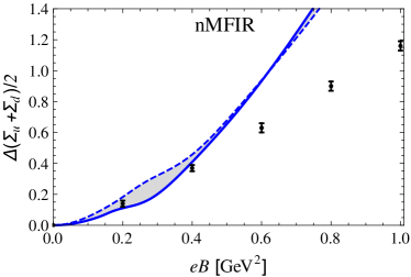
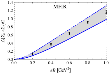
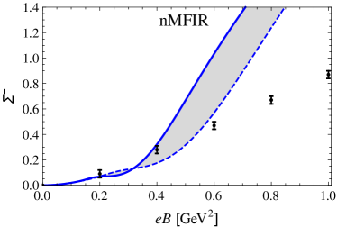
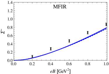
Figure 1: Results for the Lor5 form factor compared with lattice results. Upper panels: Average flavor condensate as a function of $eB$: nMFIR (left panel) and MFIR (right panel). Lower panels: difference of the up and the down quark condensates as a function of $eB$: nMFIR (left panel) and MFIR (right panel)

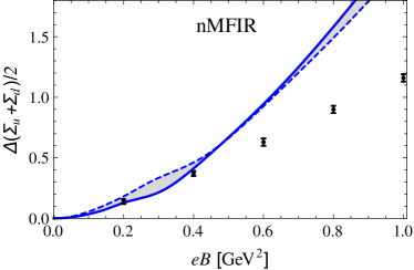
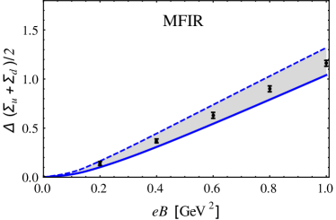
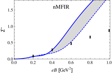
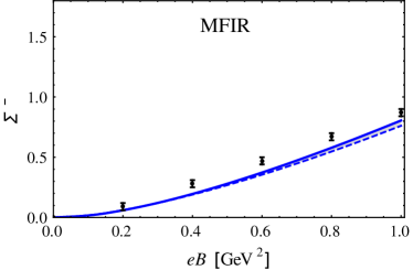
Figure 2: Results for the WS form factor with $\alpha=0.1$ compared with lattice results. Upper panels: Average flavor condensate as a function of $eB$: nMFIR (left panel) and MFIR (right panel). Lower panels: difference of the up and the down quark condensates as a function of $eB$: nMFIR (left panel) and MFIR (right panel)

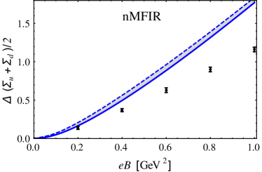
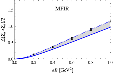
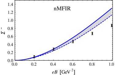
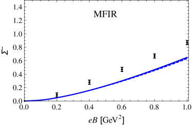
Figure 3: Results for the GR form factor compared with lattice results. Upper panels: Average flavor condensate as a function of $eB$: nMFIR (left panel) and MFIR (right panel). Lower panels: difference of the up and the down quark condensates as a function of $eB$: nMFIR (left panel) and MFIR (right panel)

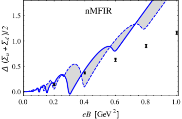
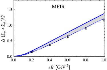
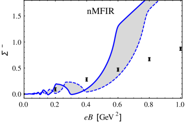
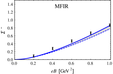
Figure 4: Results for the FD form factor with $\alpha=0.01$ compared with lattice results. Upper panels: Average flavor condensate as a function of $eB$: nMFIR (left panel) and MFIR (right panel). Lower panels: difference of the up and the down quark condensates as a function of $eB$: nMFIR (left panel) and MFIR (right panel)

We turn now to the form factor regularizations within the MFIR scheme. In this case we consider the gap equation, Eq.(III), where only the divergent integral $I^{3d}_{1}$ defined in Eq.(24) is regularized through the use of the several form factors just discussed.

In the Figs. 1-5 we present our numerical results for the behavior of the condensates as a function of $eB$ in bands for each parametrization given in Table 1. Left panels correspond to the nMFIR scheme while those on the right to the MFIR one. The dashed lines (solid lines) correspond to the higher(lower) value of $-\Phi_{0}^{1/3}$ at $B=0$ as given in Table 1 for a particular parametrization.

Our numerical results for the average quark condensate as a function of the magnetic field in the case of the Lor5 regulator are shown in the upper panels of Fig. 1 together with the lattice results of Ref.Bali:2012zg . To test the stability of our results we have used different parametrizations compatible with phenomenological bounds for $\Phi_{0}$.

In fact, they all fall within the quite narrow band indicated in the figure. In addition, we have performed the same calculations using the WS regulator with $\alpha=0.1$, and we can see in Fig.2 that again the corresponding results fall basically in the same band as those of the Lor5 regulator. Therefore, we confirm the results reported in Fig.3 of Ref.Bali:2012zg noting, in addition, that they are quite insensitive to the model parametrization. One can then conclude that the use of LorN and WS form factor regulators within the nMFIR scheme leads to a behavior of the average condensate which is in reasonable agreement with lattice results only up to $eB\sim 0.3$ GeV².

In the Fig. 3 we show the condensate as a function of $eB$ in the case of the GR regulator . One interesting aspect of using the GR form factor is that for this regulator the oscillations that appear (in nMFIR scheme) in the behavior of the condensates using the LorN and the WS form factors are not present. It should be noted, however, that the corresponding results for the condensates compare quite poorly with the lattice ones.

We can see the condensate as a function of $eB$ in the case of the FD regulator from the results of Fig.4. Non-physical oscillations arise with the FD form factor and for this regulator they are stronger than the oscillations that appear in the case of the LorN and WS form factors. We can understand these discrepancies between different form factors analyzing the behavior of the form factors as a function of the momentum. In Fig.5 we can see that FD is the sharpest function and GR in the smoothest one and the smoothness is one factor that contributes to the magnitude of the non-physical oscillations that appear when we use form factors. This is the reason why the Gaussian form factor GR do not present oscillations for the quark condensates, as shown in the left panel of Fig.3.

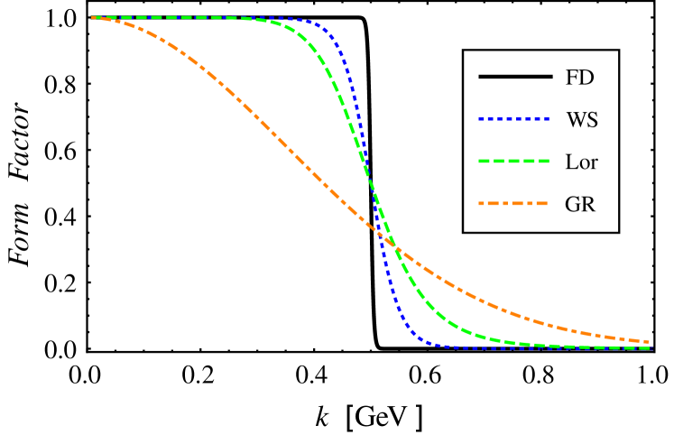
Figure 5: Behavior of the form factors FD, WS, Lor5 and GR as a functions of the momentum. In this comparison we use $\Lambda=0.5$ GeV

.

In the case of the MFIR procedure our numerical results show that for all the different shape of the form factors we obtain a good agreement with available lattice QCD calculations. This clearly shows the importance of implementing the separation of the purely magnetic part from the vacuum part, avoiding in this way the non physical oscillations that are present in nMFIR scheme.

IV.1.2 MFIR - 3D sharp cutoff regularization

In this regularization scheme the gap equation, $\frac{\partial{\cal F}}{\partial M}=0$, follows from Eq.(III). The only divergent integral $I_{1}^{3D}$, Eq.(24), is regularized introducing a non-covariant cutoff $\Lambda$ as shown in Eq.(56) of the Appendix B. In Fig. 6 we can see that this regularization procedure leads to a behavior of the average condensate which is compatible with lattice results and very similar with that ones obtained using form factors (Fig.1-Fig.4). There the upper bound of the band corresponds to $(\bar{\Phi}_{0})^{1/3}=-260$ MeV while the lower to $(\bar{\Phi}_{0})^{1/3}=-241$ MeV. We see that this band covers the lattice points.

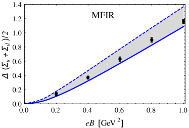
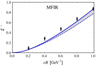
Figure 6: Average of the flavor condensate as a function of $eB$ (left panel) and difference of the up and the down quark condensates as a function of $eB$ (right panel) evaluated with MFIR using 3D cutoff method compared with lattice results.

The difference between the condensates in this regularization method can be calculated with Eq. 13, using the following definition for the condensate (magnetic part)

$$\Phi_{B}^{f}=-2N_{c}\frac{M^{3}}{8\pi^{2}}\eta(x_{f})$$ (34)

where $\eta(x_{f})$ is given by Eq. 19.

Notice that for every regularizarization based in the MFIR scheme the pure magnetic part (finite) of the condensate is given by Eq. 34.

IV.2 Covariant regularizations

As examples of these covariant regularization methods we consider the 4D sharp cutoff, proper time and Pauli-Villars. The corresponding expressions for $I_{0}^{4D}$, $I_{0}^{PT}$ and $I_{0}^{PV}$ as well as the associated parametrizations are given in Appendix B. The corresponding results for $\Delta(\Sigma_{u}+\Sigma_{d})/2$ and $\Sigma^{-}$ using a 4D sharp cutoff as a function of the magnetic field in comparison to those of the lattice are shown in Fig.7.

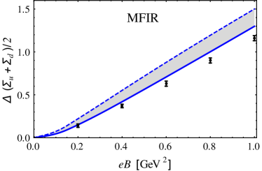
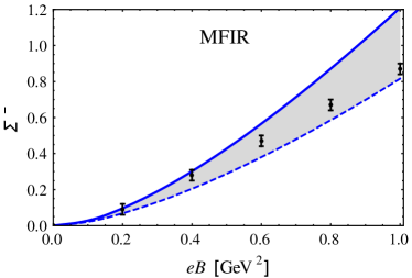
Figure 7: Average of the flavor condensate as a function of $eB$ (left panel) and difference of the up and the down quark condensates as a function of $eB$ (right panel) evaluated with MFIR using 4D cutoff method compared with lattice results.

Comparing to the results in Fig.6 we can see that the result for the difference $\Sigma^{-}$ using 4D sharp cutoff is more compatible with lattice results than the one obtained using 3D sharp cutoff. On the other hand we note that the band associated to the average condensate in the region $220$ MeV $<-\bar{\Phi}_{0}^{1/3}<260$ MeV is somewhat above the lattice values.

Alternatively, proper-time was also proposed PT and in the nMFIR scheme the integration $I_{f}$ is given by:

$$I_{f}=\frac{1}{8\pi^{2}}\int_{\frac{1}{\Lambda^{2}}}^{\infty}ds\frac{e^{-sM^{2}}}{s}|q_{f}|B\coth(|q_{f}|Bs)$$ (35)

and the condensate by:

$$\phi^{f}_{B}=-\frac{MN_{c}}{4\pi^{2}}\int_{\frac{1}{\Lambda^{2}}}^{\infty}ds\frac{e^{-sM^{2}}}{s}|q_{f}|B\coth(|q_{f}|Bs).$$ (36)

In this sense it is interesting to note that using the relations given in Appendix A the quantity $I_{f}$ to be used in the MFIR scheme can be also casted into the form

$$I_{f}=\frac{1}{8\pi^{2}}\int_{0}^{\infty}\frac{ds}{s^{2}}\ e^{-sM^{2}}\Big{[}|q_{f}|Bs\ \coth{(|q_{f}|Bs)}-1\Big{]}$$

(37)

which is the magnetic term obtained within the Schwinger formalism. In Fig. 8 we show our results using proper-time scheme, we can see that the results are similar to lattice results only for small values of $eB$.

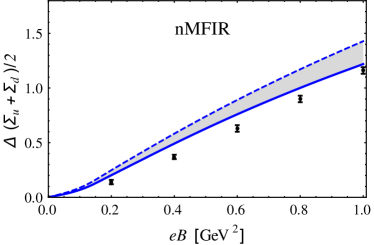
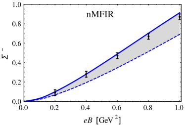
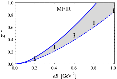
Figure 8: Results for the PT method compared with lattice results. Upper panels: Average flavor condensate as a function of $eB$: nMFIR (left panel) and MFIR (right panel). Lower panels: difference of the up and the down quark condensates as a function of $eB$: nMFIR (left panel) and MFIR (right panel).

Other very interesting regularization scheme that is used in the literature is the Pauli-Villars regularization (PV) revKlevansky ; volkov ; hatsuda ; buballa ; ruggieri . In the MFIR scheme, we have to modify the integral $I_{1}$ in Eq. 16 as given in Eq. 64. Alternatively, recent investigations focusing on the study of the effects produced by a magnetic field in quark matter are using PV regularization Cao1 ; Cao2 ; Mao1 ; Mao2 , but they do not implement the separation of the magnetic effects from the vacuum, i. e., they use a nMFIR procedure.

Following the prescriptions Cao1 ; Cao2 ; Mao1 ; Mao2 , Eq. 17 may alternatively be written replacing the integrations as

$$\sum_{k=0}^{\infty}\alpha_{k}\int\frac{dp_{3}}{2\pi}F(E_{f})\rightarrow\sum_{i=0}^{2}C_{i}\sum_{k=0}^{\infty}\alpha_{k}\int\frac{dp_{3}}{2\pi}F(E_{f},i),$$

also, we must introduce the regularized masses $M\rightarrow M^{2}_{i}=M^{2}+b_{i}\Lambda^{2}$ in the quark energy $E_{f}$. This procedure obviously rebuilds the results at $eB=0$, but does not separate explicitly the cutoff from purely magnetic contribution. The coefficients $C_{i}$ and $b_{i}$ are determined by the constraints $\sum_{i=0}^{2}C_{i}=0$ and $\sum_{i=0}^{2}C_{i}M_{i}^{2}=0$ with $b_{0}=0$, $C_{0}=1$ as indicated in revKlevansky .

The condensate in this scheme is given by

$$\Phi_{B}^{f} = -2N_{c}M\sum_{i=0}^{2}C_{i}\frac{|q_{f}|B}{2\pi}\sum_{k=0}^{\infty}\alpha_{k}$$

$$\times \int_{-\infty}^{\infty}\frac{dp_{4}}{2\pi}\int_{-\infty}^{\infty}\frac{dp_{3}}{2\pi}\frac{1}{p_{4}^{2}+p_{3}^{2}+2|q_{f}|B+M_{i}^{2}}$$

, (39)

and the integral $I_{f}$ in the nMFIR is given by

$$I_{f} = \sum_{i=0}^{2}C_{i}\int_{-\infty}^{\infty}\frac{dp_{4}}{2\pi}\int_{-\infty}^{\infty}\frac{dp_{3}}{2\pi}\left[\frac{|q_{f}|B}{2\pi}\sum_{k=0}\alpha_{k}\right.$$ (40)

$$\times\left.\frac{1}{p_{4}^{2}+p_{3}^{2}+2k|q_{f}|B+M^{2}_{i}}\right].$$

In Fig.9 we compare the two procedures: PV including MFIR and without MFIR. We clearly see that if we do not separate the magnetic contributions from the vacuum we obtain quantitative differences compared to the case where we have used the MFIR. The results obtained using Pauli-Villars regularization with MFIR are in agreement with lattice results.

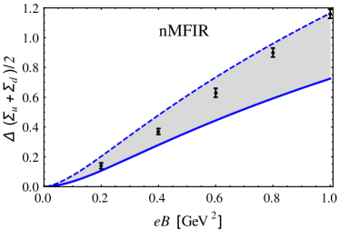
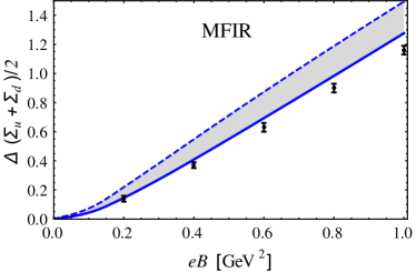
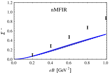
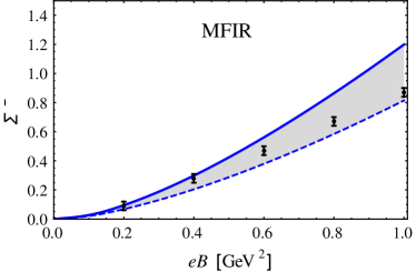
Figure 9: Results for the PV method compared with lattice results. Upper panels: Average flavor condensate as a function of $eB$: nMFIR (left panel) and MFIR (right panel). Lower panels: difference of the up and the down quark condensates as a function of $eB$: nMFIR (left panel) and MFIR (right panel).

V Conclusions

In this work we use results from lattice simulations of QCD in the presence of intense magnetic fields as a benchmark platform for comparing different regularization procedures used in the literature for the NJL type models in the context of both the so-called “magnetic field independent regularization” (MFIR) scheme, where only the non-magnetic vacuum term is regularized, and “non magnetic field independent regularization” (nMFIR) scheme, where also the magnetic terms are regularized. We implement different regularization schemes in the $SU(2)$ NJL model: Form factors, Proper Time and Pauli-Villars in both MFIR and nMFIR schemes and $3D$/$4D$ Cutoff only in the MFIR scheme. As exhaustively discussed in this work, in the MFIR scheme for the calculation of the condensates an exact separation of magnetic and non-magnetic vacuum contributions is performed before the adopted regularization prescription is applied. It is important to stress that in such case only the original vacuum term of the NJL model at $B=0$ has to be regularized. In figures 1-4 the several non-covariant form factor regularizations are compared using both nMFIR and MFIR schemes. Is is seen in figures 1 and 2 that in a nMFIR scheme the Lorentzian and Woods-Saxon procedures describe approximately the lattice data trend for the average and the difference of the flavor condensates at $eB\leq 0.3$ GeV². However, these figures already show the presence of a non-physical oscillatory behavior. The Fermi-Dirac regularization shown in Fig. (4) present a huge non-physical oscillatory behavior. As discussed in section IV, the Gaussian regulator shown in Fig. (3) has a behavior without oscillations but fails to satisfactorily reproduce the lattice data. The form factor regularizations calculated within the MFIR scheme, shown in the right panels of figures (1-4) show a satisfactory trend as compared to lattice results and, besides, no oscillatory behavior appears at all. The comparison between nMFIR with MFIR results for the form factor regularizations show clearly that the latter present much more consistent results when compared with lattice results and should be always used for reliable calculations of physical observables. In Fig.(6) the non-covariant 3D-cutoff regularization is used for the calculation of the condensates in the MFIR scheme. It is also seen in the latter figure that a good description of the trend of the lattice results is achieved and no oscillatory behavior is found.

In figures 7-9 we show results for the covariant regularizations, i. e., 4D cuttoff, Proper-Time and Pauli-Villars. Again we calculate the condensates using the covariant regularizations within the MFIR and nMFIR scheme for the Proper-Time and Pauli-Villars and only MFIR for the 4D-cutoff. It is obvious from these figures that the 4D-cutoff and the Pauli-Villars in the MFIR scheme are the best regularizations of all the covariant types. If one consider all the regularizations studied in this work, the conclusion is that the non covariant 3D-cutoff and the covariant 4D-cutoff and Pauli-Villars are the ones that better describe the lattice results for the condensates and should be chosen in any reliable calculation of physical quantities within the NJL model under strong magnetic fields. Although, in this work we focus only on the comparison of the condensates calculated within the NJL model with the corresponding lattice results, the MFIR scheme should be applied in the calculation of any physical quantity. The use of an inappropriate regularization is magnified in the calculation of several observables, e. g., the pion mass has been calculated in the literature using unreliable form factors in a nMFIR scheme and some authors have found tachyonic pions, huge oscillations of the pion mass which are, in fact, only an artifact of a bad regularization choice. Another example which highlights the importance of a correct regularization procedure is the calculation of thermodynamical quantities, since several thermodynamic quantities involve derivatives of the thermodynamic potentials, they are strongly dependent on the regularization and the existence of unphysical oscillations would certainly produce results completely unreliable. This is particularly the case when studying the color superconducting phases in the presence of a strong magnetic field where unphysical oscillations can be easily confused with actual de Haas-van Alfven oscillations.

Appendix A DERIVATION OF EQ.(18)

We start from the definition of $I_{f}$ given in Eq.(17). After substituting in this latter equation $\alpha_{k}=2-\delta_{0k}$ and using the Riemann-Hurwitz zeta function

$$\zeta(z,x)=\sum_{n=0}^{\infty}\frac{1}{(x+n)^{z}}\leavevmode\nobreak\ \leavevmode\nobreak\ ,$$ (41)

it can be written as:

$$I_{f} = \int_{-\infty}^{\infty}\frac{dp_{4}}{2\pi}\int_{-\infty}^{\infty}\frac{dp_{3}}{2\pi}\left[\frac{1}{2\pi}\zeta\left(1,\frac{p_{3}^{2}+p_{4}^{2}+M^{2}}{2|q_{f}|B}\right)\right.$$

$$- \left.\frac{|q_{f}|B}{2\pi}\frac{1}{p_{3}^{2}+p_{4}^{2}+M^{2}}\right.$$

$$- 2\int_{-\infty}^{\infty}\frac{dp_{1}}{2\pi}\left.\int_{-\infty}^{\infty}\frac{dp_{2}}{2\pi}\frac{1}{p_{1}^{2}+p_{2}^{2}+p_{3}^{2}+p_{4}^{2}+M^{2}}\right]$$

Next, from the integral representations of the zeta function

$$\int_{0}^{\infty}y^{z-1}e^{-\beta y}\coth(\alpha y) = \Gamma(z)\left[2^{z-1}\alpha^{-z}\zeta\left(z,\frac{\beta}{2\alpha}\right)\right.$$ (43)

$$- \left.\beta^{-z}\right]\leavevmode\nobreak\ ,$$

and

$$\frac{1}{A}=\int_{0}^{\infty}ds\leavevmode\nobreak\ e^{-sA}\leavevmode\nobreak\ ,$$ (44)

then Eq.(LABEL:eqb1) can be written as:

$$I_{f} = \int_{-\infty}^{\infty}\frac{dp_{4}}{2\pi}\int_{-\infty}^{\infty}\frac{dp_{3}}{2\pi}\left[\frac{|q_{f}|B}{2\pi}\int_{0}^{\infty}dye^{-(p_{3}^{2}+p_{4}^{2}+M^{2})y}\right.$$

$$\times \left.\coth(|q_{f}|By)\right.$$

$$- 2\int_{-\infty}^{\infty}\frac{dp_{1}}{2\pi}\left.\int_{-\infty}^{\infty}\frac{dp_{2}}{2\pi}\int_{0}^{\infty}dye^{-(p_{1}^{2}+p_{2}^{2}+p_{3}^{2}+p_{4}^{2}+M^{2})y}\right]$$

$$\leavevmode\nobreak\ .$$ (45)

After performing trivial Gaussian momentum integrals, one obtains the magnetic term in the Schwinger representation:

$$I_{f}=\frac{1}{8\pi^{2}}\int_{0}^{\infty}\frac{ds}{s^{2}}e^{-sM^{2}}\left[\leavevmode\nobreak\ |q_{f}|Bs\coth(|q_{f}|Bs)-1\right]\leavevmode\nobreak\ .$$ (46)

This latter integral can be calculated analytically, first we make a change of variables and write:

$$I_{f} = \frac{|q_{f}|B}{8\pi^{2}}\lim_{\epsilon\to 0}\left\{\int_{0}^{\infty}\leavevmode\nobreak\ dse^{-s\frac{M^{2}}{|q_{f}|B}}\left[\leavevmode\nobreak\ s^{-1+\epsilon}\coth(s)\right.\right.$$ (47)

$$- \left.\left.s^{-2+\epsilon}\right]\right\}\leavevmode\nobreak\ .$$

Finally, using the expressions given in the appendix of Ref.Dittrich for the integrals involved in Eq.(47):

$$\int_{0}^{\infty}ds\leavevmode\nobreak\ e^{-s\frac{M^{2}}{|q_{f}|B}}s^{-1+\epsilon}\coth(s) = -\frac{2x_{f}}{\epsilon}+2x_{f}(C+\ln 2)$$ (48)

$$+ 2\ln\Gamma(x_{f})-\ln(2\pi)$$

$$+ \ln x_{f}\leavevmode\nobreak\ ,$$

$$\int_{0}^{\infty}ds\leavevmode\nobreak\ e^{-s\frac{M^{2}}{|q_{f}|B}}s^{-2+\epsilon} = -\frac{2x_{f}}{\epsilon}+2x_{f}\ln(2x_{f})$$ (49)

$$+ 2x_{f}(C-1)\leavevmode\nobreak\ ,$$

where $C$ denotes the Euler constant, one easily obtains:

$$I_{f} = \frac{M^{2}}{8\pi^{2}}\eta(x_{f})$$

$$= \frac{M^{2}}{8\pi^{2}}\left[\frac{\ln\Gamma(x_{f})}{x_{f}}-\frac{\ln{2\pi}}{2x_{f}}+1-\left(1-\frac{1}{2x_{f}}\right)\ln x_{f}\right]$$

$$\leavevmode\nobreak\ .$$ (50)

Appendix B MODEL PARAMETRIZATIONS

The expression required to determined these quantities can be written in terms of two integrals, $I_{1}$ and $I_{2}(q^{2})$, whose explicit forms are regularization dependent. At the mean field level the gap equation leads to

$$M=m_{0}+4GMN_{c}I_{1}$$ (51)

Where $I_{1}$ is given by:

$$I_{1}=4\int\frac{d^{4}p}{(2\pi)^{4}}\frac{1}{p^{2}+M^{2}}$$ (52)

and the average condensate is given by Eq.(11). At the quadratic level the equation for the pion mass is

$$1-2GJ(-m_{\pi}^{2})=0\leavevmode\nobreak\ ,$$ (53)

where $J(q^{2})=2N_{c}\left[I_{1}+q^{2}I_{2}(q^{2})\right]$, where $I_{2}(q^{2})$ is given by

$$I_{2}(q^{2})=-2\int_{0}^{1}dz\int\frac{d^{4}p}{(2\pi)^{4}}\frac{1}{(p^{2}+M^{2}-z(z-1)q^{2})^{2}}\leavevmode\nobreak\ .$$

Finally, the pion decay constant is

$$f_{\pi}=-2\ Z_{\pi}^{1/2}\ M\ N_{c}\ I_{2}(-m_{\pi}^{2})\leavevmode\nobreak\ ,$$ (55)

where $Z_{\pi}^{-1}=-dJ(q^{2})/dq^{2}|_{q^{2}=-m_{\pi}^{2}}$.

Introducing the dimensionless quantities $M_{\Lambda}=M/\Lambda$ and $q_{\Lambda}=q/\Lambda$ the explicit expressions of $I_{1}$ and $I_{2}(q^{2})$ are as follows. For the case of 3D sharp cutoff we have

$$I^{3D}_{1} = \frac{\Lambda^{2}}{2\pi^{2}}\left[\sqrt{1+M_{\Lambda}^{2}}+M_{\Lambda}^{2}\ln{\frac{M_{\Lambda}}{1+\sqrt{1+M_{\Lambda}^{2}}}}\right]$$

(56)

$$I^{3D}_{2}(q^{2}) = \frac{1}{4\pi^{2}}\int_{0}^{1}dz\left[\frac{1}{\sqrt{1+M_{\Lambda}^{2}-z(z-1)q_{\Lambda}^{2}}}\right.$$ (57)

$$+\left.\ln{\frac{{\sqrt{M_{\Lambda}^{2}-z(z-1)\ q_{\Lambda}^{2}}}}{1+\sqrt{1+M_{\Lambda}^{2}-z(z-1)\ q_{\Lambda}^{2}}}}\right]\ ,$$

while the 3D form factor regularization read

$$I^{FF}_{1}=\frac{\Lambda^{2}}{\pi^{2}}\int_{0}^{\infty}du\frac{u^{2}U_{\Lambda}(u^{2})}{\sqrt{u^{2}+M_{\Lambda}^{2}}}$$ (58)

$$I^{FF}_{2}(q^{2})=-\frac{1}{4\pi^{2}}\int_{0}^{\infty}du\frac{u^{2}U_{\Lambda}(u^{2})}{(u^{2}+M_{\Lambda}^{2}-z(z-1)q_{\Lambda}^{2})^{3/2}}\leavevmode\nobreak\ .$$ (59)

For proper time regularization one gets

$$I^{PT}_{1} = \frac{\Lambda^{2}}{4\pi^{2}}E_{2}\left(M_{\Lambda}^{2}\right)$$ (60)

$$I^{PT}_{2}(q^{2}) = -\frac{1}{8\pi^{2}}\int_{0}^{1}dz\ E_{1}\left(M_{\Lambda}^{2}-z(z-1)\ q_{\Lambda}^{2}\right)\leavevmode\nobreak\ ,$$

where $E_{n}(x)=\int_{1}^{\infty}dt\ t^{-n}\exp{(-tx)}$ is the exponential integral function.

For $4D$ cutoff regularization one gets

$$I^{4D}_{1} = \frac{\Lambda^{2}}{4\pi^{2}}\left[1+M_{\Lambda}^{2}\ln\frac{M_{\Lambda}^{2}}{1+M^{2}_{\Lambda}}\right]\leavevmode\nobreak\ ,$$ (62)

$$I^{4D}_{2}(q^{2}) = \frac{1}{8\pi^{2}}\int_{0}^{1}dz\left[\frac{1}{1+M_{\Lambda}^{2}-z(z-1)q_{\Lambda}^{2}}\right.$$ (63)

$$+ \left.\ln{\left(\frac{M_{\Lambda}^{2}-z(z-1)\ q_{\Lambda}^{2}}{1+M_{\Lambda}^{2}-z(z-1)\ q_{\Lambda}^{2}}\right)}\right]\leavevmode\nobreak\ .$$

Finally, for Pauli-Villars regularization one gets

$$I^{PV}_{1} = \frac{\Lambda^{2}}{4\pi^{2}}\left[\left(2+M^{2}_{\Lambda}\right)\log{\left(1+2M^{-2}_{\Lambda}\right)}-2\left(1+M^{2}_{\Lambda}\right)\right.$$ (64)

$$\times \left.\log{\left(1+M^{-2}_{\Lambda}\right)}\right]$$

$$I^{PV}_{2}(q^{2}) = -\frac{1}{8\pi^{2}}\int_{0}^{1}dz\left[2\log\left(1+\frac{1}{M_{\Lambda}^{2}-z(z-1)q_{\Lambda}^{2}}\right)\right.$$ (65)

$$- \left.\log\left(1+\frac{2}{M_{\Lambda}^{2}-z(z-1)q_{\Lambda}^{2}}\right)\right].$$

where, here, $M_{\Lambda}=M/\Lambda$.

References

- (1) M.A. Stephanov, Prog. Theor. Phys. Suppl. 153, 139 (2004); M.A. Stephanov, Int. J. Mod. Phys. A 20, 4387 (2005) ; M.A. Stephanov, PoS LAT 2006, 024 (2006); O. Philipsen, Prog. Theor. Phys. Suppl. 174, 206 (2008); W. Weise, Prog. Theor. Phys. Suppl. 186, 390 (2010); K. Fukushima, T. Hatsuda, Rep. Prog. Phys. 74, 014001 (2011) ; G. Endrodi, Z. Fodor, S.D. Katz, K.K. Szabo, J. High Energy Phys. 1104, 001 (2011).
- (2) F. Karsch, Lect. Notes Phys. 583, 209 (2002).
- (3) S. Muroya, A. Nakamura, C. Nonaka, and T. Takaishi, Prog. Theor. Phys. 110, 615 (2003).
- (4) I. A. Shovkovy, Magnetic Catalysis: A Review, Lect. Notes Phys. 871, 13 (2013); M. Delia, Lect. Notes Phys. 871, 181 (2013); K. Fukushima, Lect. Notes Phys. 871, 241 (2013); N. Mueller, J. A. Bonnet and C. S. Fischer, Phys. Rev. D 89, 094023 (2014).
- (5) D. E. Kharzeev, L. D. McLerran and H. J. Warringa, Nucl. Phys. A 803, 227 (2008); V. Skokov, A. Y. Illarionov and V. Toneev, Int. J. Mod. Phys. A 24, 5925 (2009); V. Voronyuk, V. D. Toneev, W. Cassing, E. L. Bratkovskaya, V. P. Konchakovski and S. A. Voloshin, Phys. Rev. C 83, 054911 (2011).
- (6) J. O. Andersen, W. R. Naylor, A. Tranberg, Rev. Mod. Phys. 88, 025001 (2016).
- (7) V. A. Miransky and I. A. Shovkovy, Phys. Rept. 576, 1 (2015).
- (8) E.J. Ferrer, V. de la Incera, Eur. Phys. Jour. A52, 266 (2016).
- (9) U. Vogl and W. Weise, Prog. Part. Nucl. Phys. 27, 195 (1991);T. Hatsuda and T. Kunihiro, Phys. Rep. 247, 221 (1994); M. Buballa, Phys. Rept. 407, 205 (2005).
- (10) D. Ebert, K. G. Klimenko, M. A. Vdovichenko and A. S. Vshivtsev, Phys. Rev. D 61, 025005 (2000); M. A. Vdovichenko, A. S. Vshivtsev and K. G. Klimenko, Phys. Atom. Nucl. 63, 470 (2000) [Yad. Fiz. 63, 542 (2000)]. doi:10.1134/1.855661 doi:10.1134/1.855661.
- (11) D. Ebert and K. Klimenko, Nucl. Phys. A728, 203 (2003).
- (12) D. P. Menezes, M. Benghi Pinto, S. S. Avancini, A. Perez Martinez and C. Providência, Phys. Rev. C 79, 035807 (2009).
- (13) D.P. Menezes, M. Benghi Pinto, S.S. Avancini, C. Providência, Phys. Rev. C 80, 065805 (2009).
- (14) S. S. Avancini, R. L. S. Farias, M. B. Pinto, W. R. Tavares, V. S. Timóteo, Phys. Lett. B767, 247 (2017).
- (15) R.L.S. Farias, V.S. Timoteo, S.S. Avancini, M.B. Pinto, G. Krein, Eur. Phys. J. A53, 101 (2017).
- (16) S.S. Avancini, V. Dexheimer, R. L. S. Farias, V. S. Timóteo, Phys. Rev. C 97, 035207 (2018).
- (17) S. S. Avancini, W. R. Tavares, M. B. Pinto, Phys. Rev. D 93, 014010 (2016).
- (18) R.L.S. Farias, K.P. Gomes, G.I. Krein, M.B. Pinto, Phys. Rev. C 90, 025203 (2014).
- (19) M. Coppola, P. Allen, A.G. Grunfeld, N.N. Scoccola, Phys. Rev. D 96, 056013 (2017).
- (20) D.C. Duarte, P.G. Allen, R.L.S. Farias, P.H. A. Manso, R. O. Ramos, N.N. Scoccola, Phys. Rev. D 93, 025017 (2016).
- (21) P.G. Allen, A. G. Grunfeld, N. N. Scoccola , Phys. Rev. D 92, 074041 (2015).
- (22) D. C. Duarte, R.L.S. Farias , P. H.A. Manso and R. O. Ramos, Journ. Phys. Conf. Ser. 706, 052010 (2016).
- (23) G. S. Bali, F. Bruckmann, G. Endrödi, Z. Fodor, S. D. Katz, S. Krieg, A. Schäfer, and K. K. Szabó, JHEP 1202, 044 (2012).
- (24) G. S. Bali, F. Bruckmann, G. Endrödi, Z. Fodor, S. D. Katz, and A. Schäfer, Phys. Rev. D 86, 071502(R) (2012).
- (25) G. S. Bali, F. Bruckmann, G. Endrödi, S. D. Katz, and A. Schäfer, JHEP 1408, 177 (2014).
- (26) G. S. Bali, F. Bruckmann, G. Endrodi, Z. Fodor, S. D. Katz and A. Schafer, Phys. Rev. D 86, 071502 (2012).
- (27) G. Ripka, “Quarks bound by chiral fields: The quark-structure of the vacuum and of light mesons and baryons”, Oxford, UK: Clarendon Pr. (1997) 205.
- (28) H. G. Dosch and S. Narison, Phys. Lett. B 417, 173 (1998).
- (29) L. Giusti, F. Rapuano, M. Talevi and A. Vladikas, Nucl. Phys. B 538, 249 (1999).
- (30) C. McNeile, Phys. Lett. B 619, 124 (2005).
- (31) R. Gatto and M. Ruggieri, Phys. Rev. D 83, 034016 (2011).
- (32) M. Frasca and M. Ruggieri, Phys. Rev. D 83, 094024 (2011).
- (33) S. Fayazbakhsh and N. Sadooghi, Phys. Rev. D 82, 045010 (2010).
- (34) J. L. Noronha and I. A. Shovkovy, Phys. Rev. D 76, 105030 (2007); Erratum, Phys. Rev. D 86, 049901 (2012).
- (35) Jin-cheng Wang, V. de la Incera, E. Ferrer and Q. Wang, Phys. Rev. D84, 065014 (2011).
- (36) T. Inagaki, D. Kimura and T. Murata, Prog. Theor. Phys. 111, 371 (2004).
- (37) T. Mandal and P. Jaikumar, Adv. High Energy Phys. 2017, 6472909 (2017) .
- (38) M. Frasca, M. Ruggieri, Phys. Rev. D 83, 094024 (2011).
- (39) S. Klevansky, Rev. Mod. Phys. 64, 649 (1992).
- (40) M.K. Volkov, Phys. Part. Nucl. 24, 35 (1993).
- (41) T. Hatsuda, T. Kunihiro, Phys. Rep. 247 ,221(1994).
- (42) M. Buballa, Phys. Rep. 407, 205 (2005).
- (43) G. Cao, P. Zhuang, Phys. Rev. D 92, 105030 (2015).
- (44) G. Cao, A. Huang, Phys. Rev. D 93, 076007 (2016).
- (45) S. Mao, Phys. Lett. B758, 195 (2016).
- (46) S. Mao, Phys. Rev. D 94,036007 (2016).
- (47) W. Dittrich and H. Gies, Springer Tracts of Modern Physics 166, Springer-Verlag Berlin Heidelberg, 2000.