Generalized Multi-Order Total Variation for Signal Restoration

Abstract

Total Variation (TV) based regularization has been widely applied in restoration problems due to its simple derivative filters based formulation and robust performance. While first order TV suffers from staircase effect, second order TV promotes piece-wise linear reconstructions. Generalized Multi-Order Total Variation (GMO-TV) is proposed as a novel regularization method which incorporates a new multivariate Laplacian prior on signal derivatives in a non-quadratic regularization functional, that utilizes subtle inter-relationship between multiple order derivatives. We also propose a computational framework to automatically determine the weight parameters associated with these derivative orders, rather than treating them as user parameters. Using simulation results on ECG and EEG signals, we show that GMO-TV performs better than related regularization functionals.

Keywords Deblurring, signal restoration, higher order total variation, multi-order total variation, cross entropy, KL divergence, multivariate pdf, correlation matrix, $\ell_{1}$ regularization.

1 Introduction

Derivative-based regularization approach has proven to be powerful for signal restoration. The required signal is computed as a minimizer of cost that is a weighted sum of the goodness of fit to the measured data and a roughness measure, which is also known as the regularization functional. If the roughness functional is constructed as the square of derivative values summed over the entire signal support, the minimization is equivalent to Tikhonov filtering. If the roughness functional is constructed as the sum of absolute value of derivatives, the functionals are called Total Variation (TV) [1] regularization functionals. These type of functionals and the related extensions have been widely applied in signal/image restoration problems [2, 3, 4, 5, 6, 7] due to their simple filtering based formulation and robust performance in the presence of noisy measurements. TV regularization not only performs better than Tikhonov regularization [8] in terms of preserving the resolution, but also retains the benefits of filter based formulation, which supports parallelization [9, 10] and matrix free implementation with reduced storage and computational requirements.

Though first order TV [1] suffers from staircase artifacts [11, 12], higher order methods [13, 14, 15, 16, 17] yield better performance at the cost of increased computation. While second order TV [13] deals with the application of second order derivatives in TV functional, Lysaker et al. [14] included both first and second order derivatives in regularization using a parameterized function, where the parameter was adjusted manually to change contribution from different derivatives for increased restoration performance. Total Generalized Variation (TGV) [16] generalized the concept of bounded variation to arbitrary orders and its second order form [17] has been applied with state of art performance in restoration problems. The significant advantage with second order TGV (TGV2) is its coupling of first and second order terms through an auxiliary variable, which allows adaptive switching between derivative orders based on their corresponding derivative values. Generalized Total Variation (GTV) [18] is a recent extension that has been proposed to exploit the idea of group sparsity in second order signal derivatives, rather than direct sparsity of derivatives used in TV functional. The GTV functional performs better than both first and second order TV. Combined order TV [12] is another multi-order formulation proposed as a simple combination of first and second order TV functionals through user-tuned coupling parameters and demonstrated performance comparable to the state of art image restoration techniques including TGV2.

The success of using multiple order derivatives lies with the fact that the relative distribution of derivative magnitude of different orders can be exploited to retain signal sharpness in the presence of noise; this is achieved by choosing appropriate relative weights for derivative magnitudes of different orders. However, these weights are applied only on the global level after pixel-wise summation of the derivative magnitudes. In 2D, for a given pixel location, and given order, this magnitude is the norm of the result of vector differential operation. To elaborate on this with an example, consider the vectors derivative operators, ${\bf L}_{1}=[\frac{\partial}{\partial x}\;\;\frac{\partial}{\partial y}]$, ${\bf L}_{2}=[\frac{\partial^{2}}{\partial x^{2}}\;\;\frac{\partial^{2}}{\partial x^{2}}\;\;\sqrt{2}\frac{\partial^{2}}{\partial x\partial x}]$. Then the combined order TV functional of Lysaker et al. [12] can be expressed as

$$R_{ctv}(g)=\alpha_{1}\sum_{\bf r}\left\|({\bf L}_{1}g)({\bf r})\right\|_{2}+\alpha_{2}\sum_{\bf r}\left\|({\bf L}_{2}g)({\bf r})\right\|_{2}$$ (1)

The method of Bredies et al [16] uses a different approach to combine orders [16], but the contributions from derivative orders are combined in the same way as above: the weighting is applied after summing the pixel-wise derivative magnitudes. Further, all such methods leave the relative weights ($\alpha_{1}$ and $\alpha_{2}$) as user parameters.

1.1 Contribution and Outline

We are interested in developing a multiple order derivative based regularization functional where re-combining is performed directly on the derivative values without taking the magnitudes. For simplicity, we explore 1D signal restoration, where we consider the following way of combining multiple order derivatives:

$$R(g)=\sum_{r}\left\|{\bf S}(Lg)(r)\right\|_{2},$$ (2)

where ${\bf L}=\left[\frac{\partial}{\partial x},\;\frac{\partial^{2}}{\partial x^{2}},\;\cdots\;\frac{\partial^{K}}{\partial x^{K}}\right]^{T}$ is vector derivative operator, and ${\bf S}$ is a $K\times K$ full rank matrix. Our goal is to develop a probabilistic framework to construct a signal restoration method using the above form of regularization with automatic determination of the matrix ${\bf S}$. Our contributions can be summarized as given below:

1. We introduce a novel multivariate Laplacian density to model multiple order derivatives as well as their inter-dependencies. We then derive the regularization functional corresponding to the proposed density, where the interdependency is modeled by a symmetric positive definite matrix, which we call as the structure matrix ${\bf S}$.

2. We derive the proposed regularization applied on a signal $g$, as the cross entropy measure between the proposed multivariate Laplacian model, and sample multivariate density function constructed from the multi-order derivatives of the signal $g$. We call this regularization functional as the generalized multi-order total variation functional (GMO-TV).

3. Given an example signal $g$, we derive a majorization-minimization algorithm to determine ${\bf S}$ as the minimizer of KL divergence between the proposed multivariate Laplacian prior probability density modeled by ${\bf S}$ and sample multivariate density function constructed from the multi-order derivatives of the signal $g$. Interestingly, the cost minimized here is mostly identical to GMO-TV. We call this algorithm the MM-KL.

4. Next, we develop a training-based signal restoration method. Suppose we are given a set of noise-free training signals, $\{g_{1},\ldots,g_{n}\}$ and the noisy measured signal $f$ originating from an underlying signal. We need to estimate this signal, which belongs to the class represented by the model signals $\{g_{1},\ldots,g_{n}\}$. The first method determines ${\bf S}$ from $\{g_{1},\ldots,g_{n}\}$ using MM-KL and restores the required signal from $f$ by minimizing GMO-TV functional parameterized by ${\bf S}$. The minimization for $f$ is also carried out using majorization-minimization approach. We call this algorithm the MM-GMOTV.

5. Further, we develop a signal restoration method in which the required signal and the structure matrix are jointly determined as the minimizers of GMO-TV. The proposed method is constructed as an alternation between MM-KL and MM-GMOTV. We also provide a proof of convergence for this method.

6. We apply the proposed approach for 1D signal restoration on ECG and EEG signals including denoising and deblurring. The experimental results show that the proposed methods perform better than current multi-order derivative based methods, while having no requirement for tuning the model parameters as opposed to the compared methods, which leave the model parameters as user parameters.

The rest of the paper is as follows: Section 2 presents the signal restoration problem, in two view points: maximum a posteriori estimation and cross entropy penalized maximum likelihood estimation. Section 3 presents the proposed multi-variate Laplacian prior parameterized by a structure matrix and the derivation of GMO-TV functional. It also develops an algorithm to determine the structure matrix (MM-KL). Section 4 presents the training-based signal restoration using the GMO-TV functional (MM-GMOTV). Section 5 presents the training-free signal restoration approach using the GMO-TV functional. Section 6 presents some experimental results.

2 Signal restoration as MAP estimation and Cross-entropy penalized ML estimation

Let $g_{o}:\Omega\to\mathbb{R}$ be the original uncorrupted 1D discrete signal defined on finite $\Omega\subseteq\mathbb{Z}$ and $f:\Omega\to\mathbb{R}$ be the discrete measurement of $g_{o}$ given by

$$f(x)=h(x)\ast g_{o}(x)+\eta(x),\ x\in\Omega$$ (3)

where $h$ is a known linear transfer function representing the distortion and $\eta$ is the additive noise that corrupts the measurement. When $h$ is considered to be $\delta(x)$, the restoration problem becomes denoising. It is given that the pdf of distribution of noise $\eta(x)$ is $p_{Y}(y,m)$, where $m$ denotes the ideal measurable value and $y$ denotes the actual value measured by the acquisition device. It is also given that the values of the derivatives of $g_{o}$ (specific order) follows a distribution with pdf $q_{V}(v)$. With these definitions, the conditional probability for $f$ being the measured signal with the condition that the given candidate signal $g$ is the source of the measurement, can be expressed as

$$p(f|g)=\prod_{x}p_{Y}(f(x),(h*g)(x)),$$ (4)

where we have assumed that, for any two index $x_{1}$ and $x_{2}$, the noise is independently distributed.

The posterior probability of a candidate signal $g$, given measurement $f$ is

$$p(g|f)=\frac{p(f|g)p(g)}{p(f)},$$ (5)

where $p(f|g)$ is the probability of obtaining the observation $f$ given $g$, $p(g)$ is the probability distribution of $g$ and $p(f)$ is the probability distribution of $f$. The maximum a posteriori method (MAP) computes the required signal as a maximizer of the above probability with respect to $g$ as the maximization variable. Since $p(f)$ is independent of the maximization variable $g$, it can be skipped from the expression. The probability $p(g)$ is known as prior probability and is defined in terms of point-wise roughness of the signal. To maximize the above probability, we minimize its negative logarithm. The MAP based signal restoration amounts to finding $\hat{g}$ as a minimizer of negative logarithm of $p(g|f)$. In the remainder of the paper, we restrict ourself to Gaussian pdf for $p_{Y}(\cdot,m)$ which is the most commonly used assumption.

Our focus is now on investigating the form of $p(g)$ such that negative log of $p(g|f)$ becomes compatible with known forms of cost functions used in the literature for signal restoration. $p(g)$ can be expressed as

$$p(g)=\prod_{x}q_{V}((L*g)(x)),$$ (6)

where $L$ is the discrete filter implementing the derivative of a given order, and $q_{V}(\cdot)$ is the prior probability on the distribution of derivatives. Here too, we assume that the distributions of derivatives across different sample locations are independent. With this assumption, the negative log of $p(g|f)$ can be written as follows with $p_{Y}(\cdot,m)$ restricted to be Gaussian pdf:

$$J(g)=\underbrace{\frac{1}{2}\sum_{x}(((h*g)(x)-f(x))^{2}}_{D(f,g)}\underbrace{-\sum_{x}log(q_{V}((L*g)(x)))}_{R(g)}.$$ (7)

The independence assumption on the derivatives at different sample locations is clearly not true. However, well-known cost functionals used for signal restoration can be expressed using this assumption. For example, the following form of $q_{V}(\cdot)$ will give the well-known quadratic functional,

$$q_{{\mathbf{V}}}({\mathbf{v}})=\frac{1}{Z}e^{\frac{-\lambda||{\mathbf{v}}||_{2}^{2}}{2}},{\mathbf{v}}\in{\mathbb{R}}.$$ (8)

This quadratic functional is known as Tikhonov functional, which can be expressed as

$$R(g)=\lambda\sum_{x}((L*g)(x))^{2}.$$ (9)

Next, the total variation functional

$$R(g)=\lambda\sum_{x}|((L*g)(x))|,$$ (10)

is the result of using the following form of $q_{V}(\cdot)$:

$$q_{V}(v)=\frac{1}{Z}e^{\frac{-\lambda||{\mathbf{v}}||_{2}}{2}}.$$ (11)

An alternative way to get the form in the equation (7) is by summing negative log of $p(g|f)$ with a penalty term known as the cross entropy measure. Specifically,

$$J(g)=\frac{1}{2}{\sum_{x}(((h*g)(x)-f(x))^{2}}+H(p_{\scriptscriptstyle V,g},q_{\scriptscriptstyle V}),$$ (12)

where $H(p_{\scriptscriptstyle V,g},q_{\scriptscriptstyle V})$ is the cross entropy measure between $q_{\scriptscriptstyle V}$ and the sample pdf obtained from the derivatives of the candidate signal $g$. The cross entropy can be expressed as given below:

$$H(p_{\scriptscriptstyle V,g},q_{\scriptscriptstyle V})=-\int_{\bf v}p_{\scriptscriptstyle V,g}({\bf v})log[q_{\scriptscriptstyle V}({\bf v})]d{\bf v}$$ (13)

The sample pdf $p_{\scriptscriptstyle V,g}$ is expressed in the form of a Parzen window based estimator as given below:

$$p_{\scriptscriptstyle V,g}(\mathbf{v)}=\frac{1}{Z}\sum_{x}G_{\sigma}(||\mathbf{v}-(L*g)(x)||_{2}^{2})\\$$ (14)

where $G_{\sigma}$ is the Gaussian kernel with size $\sigma$, and $Z$ is a normalization constant. Substituting equation (14) in the equation (13) gives

$$H(p_{\scriptscriptstyle V,g},q_{\scriptscriptstyle V})=-\int_{\bf v}\frac{1}{Z}\sum_{x}G_{\sigma}(||\mathbf{v}-(L*g)(x)||_{2}^{2})log[q_{\scriptscriptstyle V}({\bf v})]d{\bf v}$$ (15)

Taking the integral inside the summation gives

$$H(p_{\scriptscriptstyle V,g},q_{\scriptscriptstyle V})=-\frac{1}{Z}\sum_{x}\int_{\bf v}G_{\sigma}(||\mathbf{v}-(L*g)(x)||_{2}^{2})log[q_{\scriptscriptstyle V}({\bf v})]d{\bf v}.$$ (16)

To simplify further, we take the limit $\sigma\rightarrow 0$. With this limit, the integral $\int_{\bf v}G_{\sigma}(||\mathbf{v}-(L*g)(x)||_{2}^{2})log[q_{\scriptscriptstyle V}({\bf v})]d{\bf v}$ becomes $log[q_{\scriptscriptstyle V}((L*g)(x)]$ because $G_{\sigma}(||\mathbf{v}-(L*g)(x)||_{2}^{2})$ becomes a sampling kernel for $\sigma\rightarrow 0$. Hence, the cross entropy becomes

$$H(p_{\scriptscriptstyle V,g},q_{\scriptscriptstyle V})=-\sum_{x}log[q_{\scriptscriptstyle V}((L*g)(x))].$$ (17)

This means that the $H(p_{\scriptscriptstyle V,g},q_{\scriptscriptstyle V})$ is identical to $R(g)$ introduced in the equation (7). Hence, cross entropy augmented negative log of data-Likelihood is identical to negative log of posterior probability, and hence cross entropy penalized ML estimation is the same as the MAP estimation. Needless to say, the well-known Tikhonov and total variation functionals of equations (9), and (10) can also be derived as specific cases of the cross entropy $H(p_{\scriptscriptstyle V,g},q_{\scriptscriptstyle V})$.

So far, we have reviewed two formulations that lead to cost functionals used for regularized signal restoration namely, MAP estimation, and cross entropy penalized ML (CE-ML) estimation. The advantage of the latter formulation is that, it does not assume that signal derivatives across difference sample locations are distributed independently. In the following section, we propose the GMO-TV functional parameterized by the so-called structure matrix, and derive an iterative algorithm to determine the structure matrix using cross entropy formulation.

3 Generalized Multi-Order Total Variation Functional

3.1 Multivariate Laplacian prior on signal derivatives and the corresponding regularization functional

Consider a signal $g(x)$ with derivative $\mathbf{v}_{g}(x)$ given by $\mathbf{v}_{g}(x)=\mathbf{L}(x)\ast g(x)$, where ${\bf L}$ is a vector derivative filter for derivatives upto the $K^{th}$ order and given by

$${\bf L}(x)=\left[\frac{\partial}{\partial x},\;\frac{\partial^{2}}{\partial x^{2}},\;\cdots\;\frac{\partial^{K}}{\partial x^{K}}\right]^{T},$$ (18)

To incorporate a general prior best suited for modeling long-tailed distribution observed in signal derivatives and also handle local inter-dependencies among these derivatives, we propose to use the following form of multivariate Laplacian prior:

$$q_{\mathbf{V}}(\mathbf{v})=\frac{1}{Z(K)|{\bf C}|^{\frac{1}{2}}}e^{-\sqrt{\left({\bf v}^{T}{\bf C}^{-1}{\bf v}\right)}},\mathbf{v}\in\mathbb{R}^{K},$$ (19)

where ${\bf C}$ is positive definite matrix, and $Z(K)$ is normalization constant. Next, the sample multivariate pdf estimated from the multi-order derivatives of $g$ can be expressed as

$$p_{\scriptscriptstyle V,g}(\mathbf{v)}=\frac{1}{Z_{p}}\sum_{x}G_{\sigma}(||\mathbf{v}-(L*g)(x)||_{2}^{2}),\\$$ (20)

where $Z_{p}$ is another normalization constant. Now, note that the steps used in the second part of Section 2 to derive the expression for $H(p_{\scriptscriptstyle V,g},q_{\scriptscriptstyle V})$ in the univariate case are directly extendible for the multivariate case. Hence $H(p_{\scriptscriptstyle V,g},q_{\scriptscriptstyle V})$ for the current multivariate case can be expressed as

$$H(p_{\scriptscriptstyle V,g},q_{\scriptscriptstyle V})=-\sum_{x}log[q_{\scriptscriptstyle V}(({\bf L}*g)(x))].$$ (21)

Substituting the expression of the equation (19) in the above equation gives

$$\bar{R}(g,{\bf C})=H(p_{\scriptscriptstyle V,g},q_{\scriptscriptstyle V})=-\sum_{x}\sqrt{(({\bf L}*g)(x))^{T}{\bf C}^{-1}({\bf L}*g)(x)}+\frac{1}{2}\log|{\bf C}|.$$ (22)

Here we have ignored the constant that is independent of both $g$ and ${\bf C}$. As a regularization functional applied on $g$, we ignore the term involving only ${\bf C}$ and write

$$R(g,{\bf C})=\sum_{x}\sqrt{(({\bf L}*g)(x))^{T}{\bf C}^{-1}({\bf L}*g)(x)}.$$ (23)

Since ${\bf C}^{-1}$ is a symmetric matrix, it can be written as ${\bf C}^{-1}={\bf U}{\bf D}{\bf U}^{T}$, where ${\bf U}$ is an orthonormal matrix satisfying ${\bf U}^{T}{\bf U}={\bf I}$, and ${\bf D}$ is a diagonal matrix. Hence ${\bf C}^{-1}$ can be written as ${\bf C}^{-1}={\bf S}^{T}{\bf S}$, where ${\bf S}$ is a matrix of the form

$${\bf S}=\left[\begin{array}[]{c}{\bf p}_{1}^{T}\\ {\bf p}_{2}^{T}\\ \ldots,\\ {\bf p}_{k}^{T}\end{array}\right],$$

wtih ${\bf p}_{i}$’s satisfying ${\bf p}_{i}^{T}{\bf p}_{j}=0$ for $i\neq j$, and ${\bf p}_{i}^{T}{\bf p}_{i}>0$. Substituting for ${\mathbf{C}}^{-1}$ in terms of ${\mathbf{S}}$, we get the corresponding functional $R(g,{\bf S})$ as

$$R(g,{\bf S})=\sum_{x}\|{\bf S}({\bf L}*g)(x)\|_{2}.$$ (24)

Since $|{\bf C}|=\frac{1}{|{\bf S}^{T}{\bf S}|}=\frac{1}{|{\bf S}{\bf S}^{T}|}$, $\bar{R}(g,{\bf S})$ can be written as

$$\bar{R}(g,{\bf S})=\sum_{x}R(g,{\bf S})-\frac{1}{2}\log|{\bf S}{\bf S}^{T}|.$$ (25)

3.2 Determining the structure matrix ${\bf S}$

Minimizing derivative based roughness functional helps to suppress noise; but it also leads to the loss of resolution since sharp signal variations are suppressed by minimizing derivative magnitude. In this viewpoint, the purpose of introducing multi-order derivative is the following: instead of minimizing individual derivative magnitudes, we intend to minimize the deviation from the pre-determined inter-relationship among derivatives of multiple order, which will hopefully reduce the loss of signal resolution. The inter-relationship is captured by $q_{\mathbf{V}}(\mathbf{v})$ by means of the structure matrix, and its deviation from the inter-relationship present in the candidate signal $g$ is measured by the cross entropy, $H(p_{\scriptscriptstyle V,g},q_{\scriptscriptstyle V})$.

Here, we address the problem of determining ${\bf S}$, given an example signal $\bar{g}$. An obvious approach is to determine ${\bf S}$ by minimizing $H(p_{\scriptscriptstyle V,g},q_{\scriptscriptstyle V})$ given in equation (21). This approach is also optimal in information theoretic viewpoint: it minimizes the complexity of representing the derivatives of $g$ using the pdf parameterized by ${\bf S}$ by means of cross entropy measure. Interestingly, the well-known KL divergence which is also used to estimate a parametric pdf from given set of samples coincide with cross entropy measure. The KL divergence between the pdf’s $p_{\scriptscriptstyle V,g}$ and $q_{\scriptscriptstyle V}$ is expressed as

$$D_{KL}(P||Q)= \int_{\bf v}p_{\scriptscriptstyle V,g}({\bf v})\log\left(\frac{p_{\scriptscriptstyle V,g}({\bf v})}{q_{\scriptscriptstyle V}(\bf v)}\right)d{\bf v}$$ (26)

$$= \int_{\bf v}p_{\scriptscriptstyle V,g}({\bf v})\log(p_{\scriptscriptstyle V,g}({\bf v}))d{\bf v}-\int_{\bf v}p_{\scriptscriptstyle V,g}({\bf v})\log(q_{\scriptscriptstyle V}(\bf v))d{\bf v}$$ (27)

$$= \ -H(p_{\scriptscriptstyle V,g})+H(p_{\scriptscriptstyle V,g},q_{\scriptscriptstyle V})$$ (28)

Since $H(p_{\scriptscriptstyle V,g})$ is independent of ${\bf S}$, this means that minimizing $D_{KL}(P||Q)$ with respect to ${\bf S}$ is the same as minimizing $H(p_{\scriptscriptstyle V,g},q_{\scriptscriptstyle V})$. In the following section, we develop a majorization-minimization method for determining ${\bf S}$ by minimizing $D_{KL}(P||Q)$.

Now our goal is to develop a computational method for the following minimization problem:

$${\bf S}^{*}=\arg\min_{\bf S}\bar{R}(g,{\bf S})=\arg\min_{\bf S}{R}(g,{\bf S})-\frac{1}{2}\log|{\bf S}{\bf S}^{T}|.$$ (29)

where $R(g,{\bf S})$ is as defined in equation (24). In order to make this method useful for both training-based and training-free signal restoration methods (Sections 3 and 4), we need to modify the above problem as given below:

$${\bf S}^{*}=\arg\min_{\bf S}{R}_{F}(g,{\bf S})=\arg\min_{\bf S}{R}(g,{\bf S})-\frac{1}{2}\log|{\bf S}{\bf S}^{T}|+\lambda_{F}\|{\bf S}\|_{F},$$ (30)

where $\|\cdot\|_{F}$ denotes the Frobenius norm of its matrix argument. The reason for using ${R}_{F}(g,{\bf S})$ instead of $\bar{R}(g,{\bf S})$ is that ${R}_{F}(g,{\bf S})$ is bounded below for all $g$, while $\bar{R}(g,{\bf S})$ is not bounded below if the derivatives of $g$ are not well-distributed.

Let ${\bf p}^{T}=[{\bf p}_{1}^{T}\cdots{\bf p}_{k}^{T}]$. Note that ${\bf p}_{i}^{T}$’s are the rows of ${\bf S}$. Let ${\bf v}(x)=({\bf L}*g)(x)$. Let ${\bf S}_{0}$ be the initialization towards iteratively solving the above problem. To solve the above computational problem, we adopt majorization-minimization approach. Given current estimate of the minimum, say ${\bf S}^{(k)}$, we build an ${\bf S}^{(k)}$-dependent auxiliary functional, ${R}_{F}^{(k)}(g,{\bf S},{\bf S}^{(k)})$ satisfying ${R}^{(k)}_{F}(g,{\bf S}^{(k)},{\bf S}^{(k)})$ $={R}_{F}(g,{\bf S}^{(k)})$, and ${R}^{(k)}_{F}(g,{\bf S},{\bf S}^{(k)})>{R}_{F}(g,{\bf S}^{(k)})$ for ${\bf S}\neq{\bf S}^{(k)}$. Then we compute the next refined estimate as

$${\bf S}^{(k+1)}=\arg\min_{\bf S}{R}^{(k)}_{F}(g,{\bf S},{\bf S}^{(k)}).$$ (31)

To construct the majorizer for ${R}_{F}(g,{\bf S})$, we need to find the majorizer for ${R}(g,{\bf S})$ which is the most complex part of ${R}_{F}(g,{\bf S})$. The ${\bf S}^{(k)}$-dependent majorizer for ${R}(g,{\bf S})$, denoted by ${R}^{(k)}(g,{\bf S},{\bf S}^{(k)})$ can be expressed as

$${R}^{(k)}(g,{\bf S},{\bf S}^{(k)})=\sum_{x}\frac{0.5}{\|{\bf S}^{(k)}({\bf L}*g)(x)\|_{2}}\|{\bf S}({\bf L}*g)(x)\|_{2}^{2}.$$ (32)

Based on this, the majorizer for ${R}_{F}(g,{\bf S})$ can be written as

$${R}^{(k)}_{F}(g,{\bf S},{\bf S}^{(k)})=\sum_{x}\frac{0.5}{\|{\bf S}^{(k)}({\bf L}*g)(x)\|_{2}}\|{\bf S}({\bf L}*g)(x)\|_{2}^{2}-\log|{\bf S}^{T}{\bf S}|+\lambda_{F}\|{\bf S}\|_{F}$$ (33)

To construct the algorithm based on the above majorization, we will need the expression for the gradients of ${R}^{(k)}_{F}(g,{\bf S},{\bf S}^{(k)})$ and ${R}_{F}(g,{\bf S})$, which are given in the following proposition. For notational convenience, we represent this gradient in matrix form with same size as ${\bf S}$.

Proposition 1

The gradient $\nabla_{\bf S}{R}_{F}(g,{\bf S})$ is given by

$$\nabla_{\bf S}{R}_{F}(g,{\bf S})={\bf S}{\bf A}-({\bf S}{\bf S}^{T})^{-1}{\bf S}+\lambda_{F}{\bf S}$$ (34)

where ${\bf A}=\sum_{x}\frac{1}{\|{\bf S}({\bf L}*g)(x))\|_{2}}(({\bf L}*g)(x))(({\bf L}*g)(x))^{T}$
The gradient $\nabla_{\bf S}{R}^{(k)}_{F}(g,{\bf S},{\bf S}^{(k)})$ is given by

$$\nabla_{\bf S}{R}^{(k)}_{F}(g,{\bf S},{\bf S}^{(k)})={\bf S}{\bf A}_{k}-({\bf S}{\bf S}^{T})^{-1}{\bf S}+\lambda_{F}{\bf S},$$ (35)

where ${\bf A}_{k}=\sum_{x}\frac{1}{\|{\bf S}^{(k)}(({\bf L}*g)(x))\|_{2}}(({\bf L}*g)(x))(({\bf L}*g)(x))^{T}$

Based on the gradient expression for ${R}^{(k)}_{F}(g,{\bf S},{\bf S}^{(k)})$ from the above proposition, we get the closed form expression for the minimum of ${R}^{(k)}_{F}(g,{\bf S},{\bf S}^{(k)})$ with respect to ${\bf S}$, which is given in the following proposition.

Proposition 2

The minimum of ${R}^{(k)}_{F}(g,{\bf S},{\bf S}^{(k)})$ with respect to ${\bf S}$ is given by ${\bf S}^{(k+1)}=({\bf D}_{k}+\lambda_{F}{\bf I})^{-1/2}{\bf U}_{k}^{T}$, where ${\bf D}_{k}$ and ${\bf U}_{k}$ are matrices involved in the Eigen decomposition of ${\bf A}_{k}$, i.e., ${\bf A}_{k}={\bf U}_{k}{\bf D}_{k}{\bf U}_{k}^{T}$.

Together with MM scheme expressed by equation (31), this completes the derivation of iterative algorithm for minimizing ${R}_{F}(g,{\bf S})$. For readers’ convenience, we express the full algorithm in terms of computational steps. The input ${\bf v}$ is given by ${\bf v}(x)=({\bf L}*g)(x)$
Algorithm I:    $\textrm{MM-KL}({\bf v},{\bf S}^{(0)},\lambda_{F},\epsilon)$

$$Initialization:{\bf A}_{0} =\sum_{x}\frac{1}{\left\|{\bf S}^{(0)}{\bf v}(x)\right\|_{2}}{\bf v}(x){\bf v}^{T}(x),\;k=0,\;r=1\;\;\;\;\;\;\;\;$$

$$while\;\;\;\;\;r>\epsilon\;\;do$$

$$Factorize\;\;{\bf A}_{k}={\bf U}_{k}{\bf D}_{k}{\bf U}_{k}^{T}$$

$$Update\;\;{\bf S}^{(k+1)}=({\bf D}_{k}+\lambda_{F}{\bf I})^{-1/2}{\bf U}_{k}^{T},$$

$$Compute\;\;{\bf A}_{k+1}=\sum_{x}\frac{1}{\left\|{\bf S}^{(k+1)}{\bf v}(x)\right\|_{2}}{\bf v}(x){\bf v}^{T}(x)$$

$$k\leftarrow k+1$$

$$r=\|{\bf S}^{(k)}{\bf A}_{k}-({\bf S}^{(k)}({\bf S}^{(k)})^{T})^{-1}{\bf S}^{(k)}+\lambda_{F}{\bf S}^{(k)}\|_{2}$$

$$\;\;Else\;\;return\;\;{\bf S}^{(k)}.$$

Clearly, MM-KL converges to the minimum of ${R}_{F}(g,{\bf S})$ for $\epsilon=0$. However, for practical purposes, we use small positive value $\epsilon$. Note that, calling MM-KL with $\lambda_{F}=0$ returns the minimum of $\bar{R}(g,{\bf S})$, and returns the minimum of ${R}_{F}(g,{\bf S})$ otherwise. Note that $R(g,{\mathbf{S}})$ and $R_{F}(g,{\mathbf{S}})$ are both non-differentiable when ${\mathbf{v}}(x)$ = $(\mathbf{L}\ast g)(x)$ = $\mathbf{0}$. For handling such cases, we replace $\|{\bf S}^{(k)}({\bf L}*g)(x)\|_{2}$ with the approximation $\sqrt{\epsilon+||{\bf S}^{(k)}({\bf L}*g)(x)||_{2}^{2}}$ in practice, with $\epsilon$ as a small positive constant. For notational convenience, we use the term $\|{\bf S}^{(k)}({\bf L}*g)(x)\|_{2}$ in equations, while differentiability is retained through the above mentioned approximation.

4 GMO-TV based signal restoration with training

Suppose we have a set of noise-free training signal models, $\{g_{1},\ldots,g_{n}\}$ and the noisy measured signal $f$ originating from an underlying signal, which we need to estimate, and which belongs to the class represented by the model signals $\{g_{1},\ldots,g_{n}\}$. Let ${\bf v}(x)$ denote the vector sequence obtained by augmenting the vector sequences $\{({\bf L}*g_{j})(x)\}_{j=1,\ldots,n}$ across the index $x$. We first determine ${\bf S}$ from ${\bf v}(x)$, by calling MM-KL with ${\bf S}^{(0)}={\bf I}$, $\lambda_{F}=0$, and with a sufficiently low value for $\epsilon$. Let ${\bf S}^{*}$ be the result returned by MM-KL. We then get the restored signal from $f$ by minimizing the following cost:

$$\bar{J}(g,{\bf S}^{*})=\frac{1}{2}\sum_{x}(f(x)-(h\ast g)(x))^{2}+\lambda\bar{R}(g,{\bf S}^{*}).$$ (36)

Note that, with respect to $g$, the cross entropy, $\bar{R}(g,{\bf S}^{*})$, differs from ${R}(g,{\bf S}^{*})$ only by a constant. Hence, we can as well minimize the following cost to get the required signal:

$$J(g,{\bf S}^{*})=\frac{1}{2}\sum_{x}(f(x)-(h\ast g)(x))^{2}+\lambda{R}(g,{\bf S}^{*}).$$ (37)

To express the gradient, we first define the following weight sequence based on a given signal $\bar{g}$:

$$w_{[\bar{g},{\bf S}^{*}]}(x)=\frac{1}{2\left({\|{\bf S}^{*}\left(\mathbf{L}(x)\ast\bar{g}({x})\right)\|_{2}}\right)}.$$ (38)

Based on this, we define the following $\bar{g}$-dependent operator on signal $g$:

$$({\cal Q}_{[\bar{g},{\bf S}^{*}]}g)(x)=h(-x)\ast h(x)\ast g(x)+\lambda\mathbf{L}^{T}(x)\ast\left\{w_{[\bar{g},{\bf S}^{*}]}(x)\mathbf{S}^{*T}\mathbf{S}^{*}\left[\mathbf{L}g(x)\right]\right\}$$ (39)

Note that ${\cal Q}_{[\bar{g},{\bf S}^{*}]}\left[g(x)\right]$ is a linear operator on $g$ if $g\neq\bar{g}$. If $\bar{g}$ is replaced with $g$, it becomes a non-linear operator, i.e., ${\cal Q}_{[g,{\bf S}^{*}]}\left[g(x)\right]$ is a non-linear operator on $g$. Now the gradient of $J$ at a given candidate signal $g$ can be expressed as

$$d_{[g,{\bf S}^{*}]}(x)=\nabla_{g}J(g,{\bf S}^{*})=({\cal Q}_{[g,{\bf S}^{*}]}g)(x)-h(-x)\ast f(x),$$ (40)

where the subscript in $\nabla_{g}$ signifies that fact that gradient is taken with respect to $g$. Note that $\nabla_{g}J(g,{\bf S}^{*})$ is the collection of derivatives with respect to each sample or element of $g$, and its number of elements is the same as that of $g$. Hence we represent the gradient using notational form used for signal, i.e., we denote the gradient by $d_{[g,{\bf S}^{*}]}(x)$.

The minimum for $J(g,{\bf S}^{*})$ can be obtained by solving $\nabla_{g}J(g,{\bf S}^{*})=0$. We can either use majorization-minimization (MM) approach, or nested nonlinear conjugate gradient approach (NNCG) [19] for minimizing $J(g,{\bf S}^{*})$. Although NNCG is faster than MM approach, the difference in speed will be insignificant since the current problem is in 1D; on the other hand, MM method is easier to implement. Hence use the MM approach here.

Given current estimate of minimum, say $g^{(k)}$, we build a $g^{(k)}$-dependent auxiliary functional, $J^{(k)}(g,{\bf S}^{*},g^{(k)})$ satisfying $J^{(k)}(g^{(k)},{\bf S}^{*},g^{(k)})=J(g^{(k)},{\bf S}^{*})$ and $J^{(k)}(g,{\bf S}^{*},g^{(k)})>J(g^{(k)},{\bf S}^{*})$ for $g\neq g^{(k)}$. Then we compute the next refined estimate as

$$g^{(k+1)}=\arg\min_{g}J^{(k)}(g,{\bf S}^{*},g^{(k)}).$$ (41)

$J^{(k)}(g,{\bf S}^{*},g^{(k)})$ is constructed as given below:

$$J^{(k)}(g,{\bf S}^{*},g^{(k)})=\sum_{x}(f(x)-(h\ast g)(x))^{2}+\lambda\sum_{x}w_{[g^{(k)},{\mathbf{S}}^{*}]}(x){||{\bf S}^{*}\left(\mathbf{L}(x)\ast g({x})\right)||^{2}}$$ (42)

The gradient of above cost is given by

$$d^{(k)}_{[g,{\bf S}^{*}]}(x)=\nabla_{g}J^{(k)}(g,{\bf S}^{*},g^{(k)})=({\cal Q}_{[g^{(k)},\mathbf{S}^{*}]}g)(x)-h(-x)\ast f(x).$$ (43)

The minimum of $J^{(k)}(g,{\bf S}^{*},g^{(k)})$ can be computed by solving $\nabla_{g}J^{(k)}(g,{\bf S}^{*},g^{(k)})$ = $0$.

The cost $J^{(k)}(g,{\bf S}^{*},g^{(k)})$ itself has to be solved iteratively, i.e., each step in the MM update from $g^{(k)}$ to $g^{(k+1)}$ defined in equation (41) should be solved iteratively. This is solved using the method of conjugate gradient (CG). Let $\{g^{(k)}_{l}\}_{l=0,1,\ldots}$ denote the sequence of iterates generated by this iteration. Let $g^{(k)}$ be the initialization for this CG iteration, i.e., $g^{(k)}_{0}=g^{(k)}$. If $l^{*}$ denotes the index at which the termination criterion is attained, $g^{(k+1)}$ becomes $g^{(k+1)}=g^{(k)}_{l^{*}}$. We propose to use the following termination condition: $\|\nabla_{g}J^{(k)}(g^{(k)}_{l^{*}},{\bf S}^{*},g^{(k)})\|_{2}<\epsilon_{q}$, where $\epsilon_{q}$ is a user-specified real positive number. Further, we propose to terminate the MM iteration specified by equation (41) on the attainment of condition $\|\nabla_{g}J(g^{(k)},{\bf S}^{*})\|_{2}<\epsilon_{m}$, where $\nabla_{g}J(g^{(k)},{\bf S}^{*})$ is as given in equation (40), and $\epsilon_{m}$ is an another user-specified real positive number. If the MM loop of equation (41) is initialized with $g^{(0)}$, and $\hat{g}$ is the result returned by the overall MM method with termination tolerances $\epsilon_{q}$ and $\epsilon_{m}$, we denote the action of the overall methods as $\hat{g}=\textrm{MM-GMOTV}(g^{(0)},{\bf S}^{*},\epsilon_{q},\epsilon_{m})$.

To speed-up CG iterations, we use the preconditioner based on the diagonal approximation of ${\cal Q}_{[g^{(k)},{\mathbf{S}}^{*}]}$. This diagonal approximation is multiplication by the following:

$${D}_{[g^{(k)}]}(x)=\ \sum_{y}\left(h(y)\right)^{2}+\sum_{i=1}^{4}\left(\hat{\mathbf{L}}_{i}(-x)\right)^{\boldsymbol{\cdot}2}\ast w^{(k-1)}(x),$$ (44)

where $\left(\bullet\right)^{\boldsymbol{\cdot}2}$ denotes the element-wise squaring of its filter argument, and $\hat{\mathbf{L}}_{i}(x)=\ \mathbf{p}^{T}_{i}\mathbf{L}(x)$ with $\mathbf{p}^{T}_{i}$ being the $i^{th}$ row of $\mathbf{S}^{*}$. The proposed preconditioner is the division with ${D}_{[g^{(k)}]}(x)$. As in previous section, we use the differentiable approximation for $||{\bf S}^{*}\left(\mathbf{L}(x)\ast g({x})\right)||_{2}$ in all cases.

Although the need for noise-free signals narrows-down the applicability of this method, such scenarios are not unnatural. For example, in applications where signals such as ECG, EEG, are transmitted over a communication channel, one can compute ${\bf S}^{*}$ before transmission, and use it to restore the signals received through the transmission channel. Another possibility is that, one can compute ${\bf S}^{*}$ from signals acquired using expensive low-noise equipments, and use it to restore signals that are acquired using inexpensive noisy equipments.

5 GMO-TV based signal restoration without training

5.1 Eliminating the training

To apply GMO-TV functional without the need for training signals, we propose to formulate the signal restoration problem as a joint minimization problem where both the signal, $g$, and the structure matrix, ${\bf S}$, become minimization variables. Specifically, the signal restoration becomes as given below

$$(g^{*},{\bf S}^{*})=\arg\min_{(g,{\bf S})}{J}_{F}(g,{\bf S})=\arg\min_{(g,{\bf S})}\frac{1}{2}\sum_{x}(f(x)-(h\ast g)(x))^{2}+\lambda{R}_{F}(g,{\bf S}),$$ (45)

where ${R}_{F}(g,{\bf S})$ is as given in equation (30). The restoration problem hence becomes estimating $g^{*}$ and ${\bf S}^{*}$ jointly such that they agree with each other in the sense of cross entropy, and $g^{*}$ fits the measured signal $f$ well. Note that ${R}_{F}(g,{\bf S})=\bar{R}(g,{\bf S})+\lambda_{F}\|{\bf S}\|_{F}$ is essentially the cross entropy $H(p_{\scriptscriptstyle V,g},q_{\scriptscriptstyle V})$ (except for the added Frobenius norm of ${\bf S}$), where $q_{\scriptscriptstyle V}$ is the parametric pdf expressed in terms of ${\bf S}$ (equation (19)), and $p_{\scriptscriptstyle V,g}$ is the sample pdf of the derivatives of $g$ (equation (14)). Note that $\bar{R}(g,{\bf S})$ can become unbounded below with respect to ${\bf S}$ when $g$ does not have its derivatives sufficiently distributed (example: $g=0$). This is why $\|S\|_{F}$ has been included, which makes the overall cost bounded below even for the cases when $g=0$. Note that $\lambda_{F}$ can be chosen to be arbitrary low, and the boundedness can still be ensured.

To compute the solution for the above problem, we adopt the method of block coordinate descent. Let ${\bf S}^{(0)}$ be the initialization. Then the block coordinate descent method involves the following steps with $m$ being the iteration index:

$$\mbox{Step 1}:\;\;\;\;\;\; g^{(m+1)}=\arg\min_{g}{J}_{F}(g,{\bf S}^{(m)})$$ (46)

$$\mbox{Step 2}:\;\;\;\;\; {\bf S}^{(m+1)}=\arg\min_{\bf S}{J}_{F}(g^{(m+1)},{\bf S})$$ (47)

The algorithm expressed by equations (46) and (47), belongs to the class of block-coordinate descent methods. It is known that these methods converge to a local minimum if the function is convex with respect to each block of variables according to the result of Bertsekas [20]. For our problem, this requirement is clearly satisfied, i.e., ${J}_{F}(g,{\bf S})$ is convex either with respect to $g$ with ${\bf S}$ fixed, or with respect to ${\bf S}$ with $g$ fixed. However, these minimization sub-problems cannot be computed exactly as there are no closed form solutions. Hence the convergence results of Bertsekas is not strictly applicable. In the following section, we first discuss about the iterative methods for solving these sub-problems. Then, we propose practical termination conditions for the above minimization sub-problems to ensure convergence of the overall algorithm.

5.2 Solving the subproblems

Note that, with respect to $g$ alone, the functionals $J_{F}(g,{\bf S})$ and ${J}(g,{\bf S})$ differ only by a constant. Hence, their gradients with respect to $g$ are identical, i.e., $\nabla_{g}{J}_{F}(g,{\bf S})=\nabla_{g}{J}(g,{\bf S})$, which is given in equation (40). Hence, the minimization in Step 1 can be solved by using Majorization-Minimization method. This can be done by calling MM-GMOTV with $g^{(m)}$ as the initialization for the minimization variable $g$, and with ${\bf S}^{(m)}$ as parameter for GMO-TV functional. In other words, the result of step 1, $g^{(m+1)}$, can be obtained as $g^{(m+1)}=\textrm{MM-GMOTV}(g^{(m)},{\bf S}^{(m)},\epsilon_{q},\epsilon_{m})$, with appropriately chosen termination tolerances $\epsilon_{q}$, and $\epsilon_{m}$.

Next, for solving step 2, we can use MM algorithm developed in Section 3.2. Specifically, we call MM-KL with ${\bf S}^{(m)}$ as initialization for the minimization variable ${\bf S}$, and with ${\bf v}(x)=({\bf L}*g^{(m+1)})(x)$. In other words, the result of step 2 can be obtained as ${\bf S}^{(m+1)}=\textrm{MM-KL}(({\bf L}*g^{(m+1)})(x),{\bf S}^{(m)},\lambda_{F},\epsilon_{kl})$, with appropriately chosen termination tolerance $\epsilon_{kl}$.

Note that, the iterative methods MM-GMOTV and MM-KL terminate based on the gradient norms. In our experiments, we observed a good convergence of the overall algorithm with high quality restoration results by setting the termination tolerance to be lower than $10^{-4}$. However, we are not aware of any theoretical results for the convergence of the overall iteration, when the iteration for sub-problems are terminated based on the gradient norms. In the following proposition, we provide alternative termination conditions for the sub-problem that can be met with finite number of inner iterations.

Proposition 3

The algorithm expressed by Step 1 and Step 2 in the equations (46) and (47), converges to a local minimum if the following conditions are satisfied:

$$\left|\left<g^{(m+1)}-g^{(m)},\nabla_{g}{J}_{F}(g^{(m+1)},{\bf S}^{(m)})\right>\right|<\left|\left<g^{(m+1)}-g^{(m)},\nabla_{g}{J}_{F}(g^{(m)},{\bf S}^{(m)})\right>\right|$$ (48)

$$\left|\left<{\bf S}^{(m+1)}-{\bf S}^{(m)},\nabla_{\bf S}{J}_{F}(g^{(m+1)},{\bf S}^{(m+1)})\right>\right|<\left|\left<{\bf S}^{(m+1)}-{\bf S}^{(m)},\nabla_{\bf S}{J}_{F}(g^{(m+1)},{\bf S}^{(m)})\right>\right|$$ (49)

6 Experimental results

To evaluate the effectiveness of the proposed regularization, GMO-TV, we used ECG and EEG signals from MIT-BIH databases [21]. We tested the effectiveness of the proposed GMO-TV approach in two variations: in the first form, we used first and second order derivatives, and in the second form, we used first to fourth order derivatives. We denote the first form by GMO-TV2 and the second form by GMO-TV4. The derivatives were implemented using the discrete filters [1 -1], [1 -2 1], [-1 3 -3 1] and [1 -4 6 -4 1]. The choice of fourth order as the highest order derivative is ad-hoc and the limit is allowable complexity. The corresponding iterative versions, where training is eliminated, is referred to as IGMO-TV2 and IGMO-TV4. We compared our proposed approaches against the state of art TGV [17] and the recent GTV [18]. We also compared with the classic TV versions, denoted as TV1 and TV2. To demonstrate the importance of combining higher order derivative with lower ones, we also implemented two other variations: third and fourth order total variations, denoted by TV3, and TV4. To measure the restoration performance in our experiments, we used ISNR defined as

$$\mathrm{ISNR}=20\log_{10}\left(\frac{||g-f||_{2}}{||g-\hat{g}||_{2}}\right)$$ (50)

where $\hat{g}$ is the restored image, $f$ is the distorted input image and $g$ is the original image. For all cases, the tuning parameters including $\lambda$ were selected for each method to get the highest ISNR. The number of iterations was set large enough for TGV and GTV to ensure convergence in all experiments. In the case of GMO-TV2 and GMO-TV4 formulations with training samples, the stopping condition for MM iterations was gradient norm falling below $10^{-6}$.

For implementing the training-free version, the termination conditions for the sub-problem of step 1 and step 2 (equations (46) and (47) were set as $\left\|\nabla_{g}{J}_{F}(g^{(m+1)},{\bf S}^{(m)})\right\|_{2}<\epsilon_{a}$ and $\left\|\nabla_{\bf S}{J}_{F}(g^{(m+1)},{\bf S}^{(m+1)})\right\|_{2}<\epsilon_{a}$ which we found to yield better results compared to conditions given in the Proposition 3. For all experiments, $\epsilon_{a}$ was set to $10^{-6}$. Note that the conditions we used are much stronger than the ones given in Proposition 3.

In the first experiment, we considered denoising of ECG signals corrupted by additive white gaussian noise (AWGN) with the noise variances adjusted to match the listed SNR values. The comparison results are given in Table 1. For the training mode, the structure matrix S was generated using samples of ECG record 16272 from the MIT-BIH Normal Sinus Rhythm database [22]. For generating test signal, 2048 samples from ECG record 16265 was taken and divided into four segments, each of 512 samples. Each experiment was performed on all four segments and the results averaged to get accurate performance results for all algorithms. The results show that GMO-TV4 gives the best performance in all cases followed closely by GMO-TV2, IGMO-TV4 and IGMO-TV2. It should be emphasized that the training-free versions, GMO-TV4 and IGMO-TV2 are clearly superior to TGV, and GTV. They are also superior to the single order total variations, TV1—TV4.

‘ SNR TV1 TV2 TV3 TV4 GMO-TV4 GMO-TV2 IGMO-TV4 IGMO-TV2 TGV GTV 25 3.43 3.18 2.99 2.52 4.06 3.97 3.83 3.98 3.20 3.36 20 4.06 3.75 3.68 3.25 4.86 4.64 4.82 4.67 3.74 4.04 15 4.90 4.30 4.46 3.94 5.92 5.45 5.80 5.43 4.37 4.88 10 6.54 5.83 5.69 5.29 7.80 7.30 7.46 7.19 5.92 6.46

Table 1: Denoising Normal Sinus Rhythm ECG Signal

In second experiment, we consider the deblurring problem. We tested both training-based and training-free methods. For generating test measurements, we consider the same set of ECG signals used for the first experiment, along with a new set of EEG signals. We used EEG record chb01_02_edfm from CHB-MIT Scalp EEG database [23] for training and four 512 length segments from chb01_01_edfm record for testing. We considered four levels of Gaussian blurring by setting the variance of blurring kernel, $\sigma_{b}^{2}$ appropriately. Also for each blurring level, we considered four levels of AWGN noise. The noise levels were chosen such that the corresponding BSNR attains dB values $\{10,15,20,25\}$ where BSNR is defined as follows [24]:

$$\mathrm{BSNR}=\mathrm{var}(h\ast g)/\sigma_{\eta}^{2}$$ (51)

The results for ECG and EEG test signals are presented in the Table 2 and Table 3 respectively.

Table 2: Deblurring Normal Sinus Rhythm ECG Signal

BSNR	$\sigma^{2}_{b}$	TV1	TV2	TV3	TV4	GMO-TV4	GMO-TV2	IGMO-TV4	IGMO-TV2	TGV
25	1	5.73	5.88	8.76	7.95	9.61	9.95	8.96	9.97	7.53
	2	5.97	7.22	10.42	9.76	10.98	12.11	10.99	11.28	9.45
	4	7.72	9.27	11.39	10.79	12.81	13.57	11.59	12.62	8.68
	6	7.65	9.28	9.87	8.82	12.05	12.38	10.04	12.61	6.59
20	1	2.69	4.20	7.30	6.33	7.85	8.09	7.37	8.07	4.75
	2	5.25	6.88	8.92	8.85	9.76	10.42	9.22	9.85	7.06
	4	6.31	8.14	9.13	8.52	10.80	11.06	9.90	11.13	6.64
	6	6.97	8.19	8.45	7.66	10.95	10.96	7.35	9.83	5.71
15	1	2.65	3.54	5.40	4.90	6.20	6.46	4.17	4.28	3.11
	2	4.46	5.71	7.16	6.86	8.30	8.46	7.66	8.51	4.86
	4	5.35	6.38	6.57	6.06	8.48	8.32	7.81	8.28	5.29
	6	5.45	6.18	5.97	5.50	8.47	8.08	6.49	7.82	3.76
10	1	3.00	3.62	4.02	3.62	5.53	5.34	1.71	3.37	2.30
	2	3.52	4.42	4.52	3.85	6.37	6.30	3.86	6.00	3.01
	4	4.34	4.79	4.70	4.10	6.77	6.44	6.46	5.64	3.65
	6	3.82	4.02	3.83	3.35	6.12	5.53	6.61	5.26	2.55

Table 3: Deblurring Scalp EEG Signal

BSNR	$\sigma^{2}_{b}$	TV1	TV2	TV3	TV4	GMO-TV4	GMO-TV2	IGMO-TV4	IGMO-TV2	TGV
25	1	1.48	2.37	2.82	2.49	2.81	2.77	2.34	2.42	2.58
	2	1.10	2.74	3.06	3.07	3.12	2.84	2.72	2.81	2.95
	4	1.55	3.05	3.32	3.33	3.46	3.24	3.50	3.38	3.47
	6	1.25	2.61	2.72	2.81	2.77	2.64	3.31	3.08	2.83
20	1	0.29	1.78	1.73	1.8	1.99	1.82	1.18	1.52	1.51
	2	0.72	2.23	2.33	2.41	2.44	2.21	1.94	2.08	2.35
	4	0.96	2.21	2.40	2.42	2.48	2.29	2.98	2.81	2.78
	6	1.29	2.52	2.68	2.66	2.59	2.43	2.27	2.27	2.21
15	1	0.57	1.41	1.45	1.47	1.66	1.57	0.32	1.25	1.43
	2	1.08	2.16	2.36	2.42	2.49	2.31	1.71	2.15	2.00
	4	1.46	2.47	2.61	2.62	2.63	2.50	2.31	2.24	2.33
	6	1.27	2.13	2.18	2.14	2.29	2.21	2.20	2.25	2.27
10	1	1.73	2.54	2.59	2.57	2.76	2.58	0.95	1.78	1.58
	2	1.70	2.46	2.52	2.47	2.72	2.56	1.68	2.20	2.88
	4	1.99	2.52	2.66	2.59	2.68	2.63	2.63	2.83	2.59
	6	1.80	2.46	2.53	2.49	2.49	2.42	2.52	2.68	2.50

The results offer some interesting insights into the working of proposed approaches. While GMO-TV2 and IGMO-TV2 utilizing first and second order derivatives perform better at high BSNR values for ECG restoration, GMO-TV4 and IGMO-TV4 perform better at lower BSNR values. This indicates that higher order derivatives are robust to noise, as seen in the denoising experiment. Similarly at high BSNR values, IGMO-TV2 is able to give performance comparable to learning based GMO-TV4 and GMO-TV2 or even better in some cases. This indicates that training from noise-free samples helps in increased performance only for measurements at high noise levels. In other cases, the measurements themselves are sufficient for building the structure matrix ${\mathbf{S}}$. Furthermore in all cases, IGMO-TV2 and IGMO-TV4 perform better than other TV based functionals including TGV, and GTV, demonstrating the power of our formulation even without any training samples. Figure 1 shows the restoration result with ECG signal corresponding to BSNR =25 and $\sigma_{b}^{2}$=4.

While ECG signals have a discernible structure and the restoration results from Table 2 indicate that the proposed approaches can utilize the same with or without training samples, exploiting the signal structure in EEG signals is much more challenging. The restoration results in Table 3 show that the proposed approaches give better performance than higher order TV as well as TGV in most cases. But unlike the case of ECG, where the proposed approaches gave around 2-4dB improvement over other TV functionals, the difference in ISNR between the techniques is around 0.1-1dB in the case of EEG. This is because of the fact that EEG signals are not as structured as ECG signals. Besides, TGV has an advantage that it is spatially adaptive because of the auxiliary variable involved in its definition. Nevertheless, all four variants of the proposed method including the training-free ones perform better than TGV in most cases.

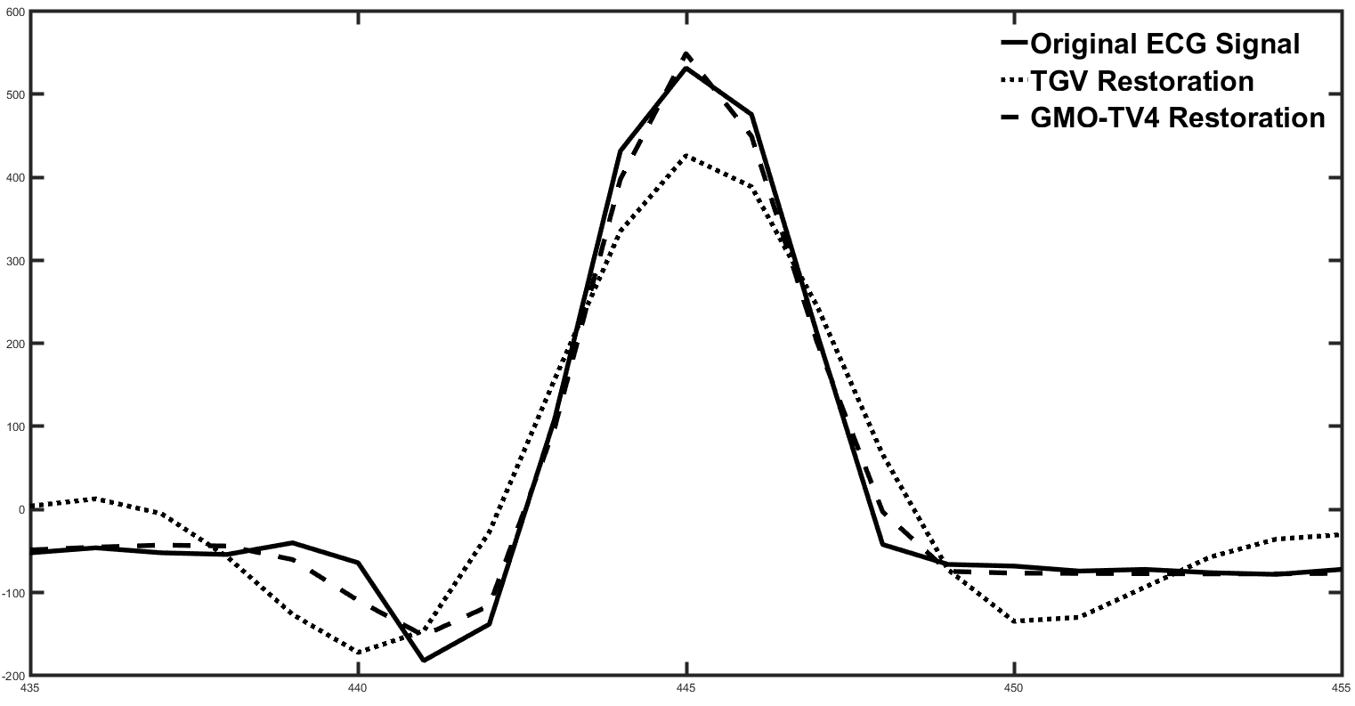
Figure 1: Deconvolution of ECG Signal (BSNR=25, $\sigma_{b}^{2}$=4)

7 Conclusion

We proposed a novel total variation based regularization functional named Generalized Multi-Order Total Variation (GMO-TV) that exploits dependencies among multiple order signal derivatives. We derived the functional from cross-entropy formulation by adopting a form of multivariate Laplacian prior probability for multiple order signal derivatives. The new prior allows the regularization functional to be adaptive to the patterns of intensity variations that are specific to the class of signals under consideration. The adaptivity is achieved by the means of a structure matrix either built via training, or estimated jointly along with the required signal via minimization. We demonstrated, using experimental examples, that GMO-TV outperforms standard TVs as well as TGV and GTV functionals with or without training.

Appendix

Proof of proposition 1

Let ${\bf p}=[{\bf p}_{1}^{T}\;{\bf p}_{2}^{T}\;\dots\bf p_{K}^{T}]^{T}$, where ${\bf p}_{i}$’s are vectors of size $K\times 1$ such that ${\bf S}=\left[{\bf p}_{1}\;{\bf p}_{2}\;\ldots\;{\bf p}_{K}\right]^{T}$. For notational convenience in deriving the algorithm, we re-express ${R}_{F}(g,{\bf S})$ in terms of ${\bf p}$ and ${\bf v}(x)$ as given below:

$$Z({\bf p},{\bf v})=\sum_{x}\sqrt{\sum_{i=1}^{K}({\bf p}_{i}^{T}{\bf v}(x))^{2}} +\frac{1}{2}\lambda_{F}\|{\bf p}\|_{2}^{2}$$ (52)

$$-\frac{1}{2}\log(\det|\left[{\bf p}_{1}\;{\bf p}_{2}\;\ldots\;{\bf p}_{K}\right]^{T}\left[{\bf p}_{1}\;{\bf p}_{2}\;\ldots\;{\bf p}_{K}\right]|)$$

Since the vectors ${\bf p}_{i}$’s are orthogonal, we get

$$Z({\bf p},{\bf v})=\sum_{x}\sqrt{\sum_{i=1}^{K}({\bf p}_{i}^{T}{\bf v}(x))^{2}}-\frac{1}{2}\log(\prod_{i=1}^{K}||\mathbf{p}_{i}||_{2}^{2})+\frac{1}{2}\lambda_{F}\sum_{i=1}^{K}||\mathbf{p}_{i}||_{2}^{2}$$ (53)

Taking gradient of $Z({\bf p},{\bf v})$ with respect to each ${\bf p}_{i}$ gives

$$\nabla_{{\bf p}_{i}}Z({\bf p},{\bf v})=\sum_{x}\frac{1}{\sqrt{\sum_{j=1}^{K}({\bf p}_{j}^{T}{\bf v}(x))^{2}}}{\bf v}(x){\bf v}^{T}(x)\mathbf{p}_{i}-\frac{{\bf p}_{i}}{\|\mathbf{p}_{i}\|_{2}^{2}}+\lambda_{F}\mathbf{p}_{i}$$ (54)

Let $\nabla_{\bf S}\bar{R}(g,{\bf S})$ denote gradient with respect to whole ${\bf S}$ in matrix form. Then

$$\nabla_{\bf S}\bar{R}(g,{\bf S})=\left[\nabla_{{\bf p}_{1}}Z({\bf p},{\bf v})\ldots\nabla_{{\bf p}_{K}}Z({\bf p},{\bf v})\right]^{T}$$ (55)

Combining the equations (54) and (55) gives $\nabla_{\bf S}\bar{R}(g,{\bf S})={\bf S}{\bf A}-({\bf S}{\bf S}^{T})^{-1}{\bf S}+\lambda_{F}{\bf S}$, where ${\bf A}$ = ${\sum\limits_{x}}\frac{1}{\|{\bf S}(({\bf L}*g)(x))\|_{2}}(({\bf L}*g)(x))(({\bf L}*g)(x))^{T}$. Using similar steps, we get gradient for $\bar{R}^{(k)}(g,{\bf S},{\bf S}^{(k)})$ as given below:

$$\nabla_{\bf S}\bar{R}^{(k)}(g,{\bf S},{\bf S}^{(k)})={\bf S}{\bf A}_{k}-({\bf S}{\bf S}^{T})^{-1}{\bf S}+\lambda_{F}{\bf S},$$ (56)

where ${\bf A}_{k}={\sum\limits_{x}}\frac{1}{\|{\bf S}^{(k)}({\bf L}*g)(x))\|_{2}}({\bf L}*g)(x))({\bf L}*g)(x))^{T}$

Proof of proposition 2

To minimize $\bar{R}^{(k)}(g,{\bf S},{\bf S}^{(k)})$, we equate the gradient to zero:

$${\bf S}{\bf A}_{k}-({\bf S}{\bf S}^{T})^{-1}{\bf S}+\lambda_{F}{\bf S}={\bf 0}$$

Using the fact that ${\bf A}_{k}$ is symmetric, re-write the above equation for individual rows of ${\bf S}$ as given below:

$$\mathbf{A}_{k}\mathbf{p}_{i}-\frac{1}{||\mathbf{p}_{i}||_{2}^{2}}\mathbf{p}_{i}+\lambda_{F}\mathbf{p}_{i}=0,\;i=1,\ldots,K.$$ (57)

The above equation implies that $\mathbf{p}_{i}$ are of the form $\mathbf{p}_{i}=\beta_{i}{\bf e}_{i}$ where ${\bf e}_{i}$ is the $i$th Eigen vector of $\mathbf{A}_{k}$ and $\beta_{i}$ is non-negative factor. Substituting this in the above equation gives

$$\beta_{i}\eta_{i}\mathbf{e}_{i}-\frac{1}{\beta_{i}^{2}}\beta_{i}\mathbf{e}_{i}+\lambda_{F}\beta_{i}\mathbf{e}_{i}=0,\;\;i=1,\ldots,K.$$ (58)

where $\eta_{i}$ is the corresponding Eigen value. The above equation gives $\beta_{i}=\frac{1}{\sqrt{\eta_{i}+\lambda_{F}}}$. This means that if ${\bf S}^{(k+1)}$ be the minimum of ${R}^{(k)}_{F}(g,{\bf S},{\bf S}^{(k)})$, then ${\bf S}^{(k+1)}=({\bf D}_{k}+\lambda_{F})^{-1/2}{\bf U}_{k}^{T}$ where ${\bf D}_{k}$ and ${\bf U}_{k}$ are the matrices involved in the Eigen decomposition of ${\bf A}_{k}$, i.e., ${\bf A}_{k}={\bf U}_{k}{\bf D}_{k}{\bf U}_{k}^{T}$.

Proof of proposition 3

Let ${\bf p}$ denote the rows of ${\bf S}$ stacked vertically and let ${\bf g}$ denote the samples of $g$ in vector form. Let ${\bf y}=[{\bf g}^{T}{\bf p}^{T}]^{T}$. Let $J_{v}({\bf y})$ is the function defined on ${\bf y}$ such that $J_{v}({\bf y})=J_{F}(g,{\bf S})$. Let ${\bf g}_{m}$ denote the vector corresponding to $g^{(m)}$ and let ${\bf p}_{m}$ denote the vector corresponding to ${\bf S}^{(m)}$. Let ${\bf y}_{2m-1}=[{\bf g}^{T}_{m}\;\;{\bf p}^{T}_{m-1}]^{T}$ and ${\bf y}_{2m}=[{\bf g}^{T}_{m}\;\;{\bf p}^{T}_{m}]^{T}$. Then ${\bf y}_{l=1,2,\ldots}$ denotes the sequence of iterates generated by the algorithm. Note that ${\bf d}_{l-1}={\bf y}_{l}-{\bf y}_{l-1}$ is the search direction at the point ${\bf y}_{l-1}$. Note that for odd $l$, ${\bf d}_{l}$ is non-zero only for the variable ${\bf p}$; similarly, for even $l$, ${\bf d}_{l}$ is non-zero only for the variable ${\bf g}$. Hence for any $l$, ${\bf d}_{l}$ is non-zero for parts corresponding to only one of the variables in $\{{\bf g},{\bf p}\}$. Further, note that the function $J_{v}({\bf y})$ is convex with respect to any one of the variables in $\{{\bf g},{\bf p}\}$. The last two statements imply that all ${\bf d}_{l}$’s are descent directions. For each descent direction ${\bf d}_{l}$, the update ${\bf y}_{l}={\bf y}_{l-1}+{\bf d}_{l-1}$ can be considered as a result of line search.

Then according to Zoutendijk Lemma [25], such a series of line searches along descent directions converge to a local minimum, if the following conditions are satisfied: (1) the sub-level set of $J_{v}({\bf y})$ for initialization ${\bf y}_{0}$ is bounded; (2) the gradient of $J_{v}({\bf y})$ is Lipschitz continuous; (3) the line search satisfies Wolfe’s condition, i.e.,

$$\left|{\bf d}_{l}^{T}\nabla_{\bf y}J_{v}({\bf y}_{l})\right|<\left|{\bf d}_{l}^{T}\nabla_{\bf y}J_{v}({\bf y}_{l-1})\right|$$ (59)

Since the function $J_{v}({\bf y})$ is bounded below, the first condition is satisfied. Also, the gradient is obviously Lipschitz continuous. Now, note that the condition given in the equation (59), can be written in two forms for odd and even values of $l$ as given below:

$$\left|({\bf g}_{m}-{\bf g}_{m-1})^{T}\nabla_{\bf g}J_{v}\left(\left[{\bf g}_{m}^{T}\;\;{\bf p}_{m-1}^{T}\right]^{T}\right)\right| <\left|({\bf g}_{m}-{\bf g}_{m-1})^{T}\nabla_{\bf g}J_{v}\left(\left[{\bf g}_{m-1}^{T}\;\;{\bf p}_{m-1}^{T}\right]^{T}\right)\right|$$ (60)

$$\left|({\bf p}_{m}-{\bf p}_{m-1})^{T}\nabla_{\bf g}J_{v}\left(\left[{\bf g}_{m}^{T}\;\;{\bf p}_{m}^{T}\right]^{T}\right)\right| <\left|({\bf p}_{m}-{\bf p}_{m-1})^{T}\nabla_{\bf g}J_{v}\left(\left[{\bf g}_{m}^{T}\;\;{\bf p}_{m-1}^{T}\right]^{T}\right)\right|$$ (61)

Rewriting the above equations in terms of the original variables $g$ and ${\bf S}$ by taking into account the dependence of the sub-parts of $J_{F}(g,{\bf S})$ on the variables $g$ and ${\bf S}$, we get the conditions of the Proposition 3.

References

- [1] Leonid I. Rudin, Stanley Osher, and Emad Fatemi. Nonlinear total variation based noise removal algorithms. Physica D: Nonlinear Phenomena, 60(1 4):259 – 268, 1992.
- [2] Om Prakash Yadav and Shashwati Ray. Smoothening and segmentation of ECG signals using total variation denoising-minimization-majorization and bottom-up approach. Procedia Computer Science, 85:483 – 489, 2016.
- [3] Kwang Jin Lee and Boreom Lee. Sequential total variation denoising for the extraction of fetal ECG from single-channel maternal abdominal ECG. Sensors, 16(7):1020, 2016.
- [4] Antonin Chambolle. An algorithm for total variation minimization and applications. Journal of Mathematical Imaging and Vision, 20(1):89–97, 2004.
- [5] T. F. Chan and Chiu-Kwong Wong. Total variation blind deconvolution. IEEE Transactions on Image Processing, 7(3):370–375, 1998.
- [6] N. Dey, L. Blanc-Feraud, C. Zimmer, Z. Kam, J. C. Olivo-Marin, and J. Zerubia. A deconvolution method for confocal microscopy with total variation regularization. In IEEE International Symposium on Biomedical Imaging: Nano to Macro, pages 1223–1226 Vol. 2, 2004.
- [7] Weihong Li, Quanli Li, Weiguo Gong, and Shu Tang. Total variation blind deconvolution employing split bregman iteration. Journal of Visual Communication and Image Representation, 23(3):409 – 417, 2012.
- [8] A. N. Tikhonov and V. Y. Arsenin. Solution of ill-posed problems. V.H. Winston, Washington, DC, 1977.
- [9] T. Pock, M. Unger, D. Cremers, and H. Bischof. Fast and exact solution of total variation models on the GPU. In IEEE Computer Society Conference on Computer Vision and Pattern Recognition Workshops, pages 1–8, 2008.
- [10] Xun Jia, Yifei Lou, Ruijiang Li, William Y. Song, and Steve B. Jiang. GPU-based fast cone beam CT reconstruction from undersampled and noisy projection data via total variation. Medical Physics, 37(4):1757–1760, 2010.
- [11] Wolfgang Ring. Structural properties of solutions to total variation regularization problems. ESAIM: Mathematical Modelling and Numerical Analysis, 34:799–810, 2000.
- [12] K. Papafitsoros and C. B. Schönlieb. A combined first and second order variational approach for image reconstruction. Journal of Mathematical Imaging and Vision, 48(2):308–338, 2014.
- [13] O. Scherzer. Denoising with higher order derivatives of bounded variation and an application to parameter estimation. Computing, 60(1):1–27, 1998.
- [14] Marius Lysaker and Xue-Cheng Tai. Iterative image restoration combining total variation minimization and a second-order functional. International Journal of Computer Vision, 66(1):5–18, 2006.
- [15] Maïtine Bergounioux and Loic Piffet. A second-order model for image denoising. Set-Valued and Variational Analysis, 18(3):277–306, Dec 2010.
- [16] Kristian Bredies, Karl Kunisch, and Thomas Pock. Total generalized variation. SIAM J. Img. Sci., 3(3):492–526, 2010.
- [17] Florian Knoll, Kristian Bredies, Thomas Pock, and Rudolf Stollberger. Second order total generalized variation (TGV) for MRI. Magnetic Resonance in Medicine, 65(2):480–491, 2011.
- [18] I. W. Selesnick. Generalized total variation: Tying the knots. IEEE Signal Processing Letters, 22(11):2009–2013, Nov 2015.
- [19] D. G. Skariah and M. Arigovindan. Nested conjugate gradient algorithm with nested preconditioning for non-linear image restoration. IEEE Transactions on Image Processing, 26(9):4471–4482, Sept 2017.
- [20] Dimitri P Bertsekas. Nonlinear programming. Athena scientific Belmont, 1999.
- [21] Ary L. Goldberger, Luis A. N. Amaral, Leon Glass, Jeffrey M. Hausdorff, Plamen Ch. Ivanov, Roger G. Mark, Joseph E. Mietus, George B. Moody, Chung-Kang Peng, and H. Eugene Stanley. Physiobank, physiotoolkit, and physionet. Circulation, 101(23):e215–e220, 2000.
- [22] Mit-bih nsrdb, https://www.physionet.org/physiobank/database/nsrdb/.
- [23] Chb-mit db, https://www.physionet.org/physiobank/database/chbmit/.
- [24] S. Lefkimmiatis, J. P. Ward, and M. Unser. Hessian schatten-norm regularization for linear inverse problems. IEEE Transactions on Image Processing, 22(5):1873–1888, 2013.
- [25] J. Nocedal and S. Wright. Numerical Optimization. Springer Series in Operations Research and Financial Engineering. Springer New York, 2006.