FLightNNs: Lightweight Quantized Deep Neural Networks for Fast and Accurate Inference

Abstract.

To improve the throughput and energy efficiency of Deep Neural Networks (DNNs) on customized hardware, lightweight neural networks constrain the weights of DNNs to be a limited combination (denoted as $k\in\{1,2\}$) of powers of 2. In such networks, the multiply-accumulate operation can be replaced with a single shift operation, or two shifts and an add operation. To provide even more design flexibility, the $k$ for each convolutional filter can be optimally chosen instead of being fixed for every filter. In this paper, we formulate the selection of $k$ to be differentiable, and describe model training for determining $k$-based weights on a per-filter basis. Over 46 FPGA-design experiments involving eight configurations and four data sets reveal that lightweight neural networks with a flexible $k$ value (dubbed FLightNNs) fully utilize the hardware resources on Field Programmable Gate Arrays (FPGAs), our experimental results show that FLightNNs can achieve 2$\times$ speedup when compared to lightweight NNs with $k=2$, with only 0.1% accuracy degradation. Compared to a 4-bit fixed-point quantization, FLightNNs achieve higher accuracy and up to 2$\times$ inference speedup, due to their lightweight shift operations. In addition, our experiments also demonstrate that FLightNNs can achieve higher computational energy efficiency for ASIC implementation.

1. Introduction

Emerging vision, speech and natural language applications have widely adopted deep learning models and, as a result, have achieved state-of-the-art accuracy. Furthermore, recent industrial efforts have focused on implementing the models on mobile devices (NNA, [n. d.]). However, real-time applications based on these deep models may incur unacceptably large latencies and can easily drain the battery on energy-limited devices. For example, smartphones can only run the AlexNet-based object detection for one hour (Yang et al., [n. d.]). Therefore, prior research has proposed model compression techniques including pruning and quantization to satisfy the stringent energy and speed requirements (Lin et al., 2016).

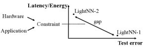
Figure 1. A discrete Pareto-optimal curve for LightNN models $w.r.t.$ test error and latency/energy. More continuous Pareto-optimal points are needed to adapt to the latency/energy constraints determined by the hardware and application.

One of the recently proposed quantization approaches, LightNN, constrains the weights of DNNs to be a sum of $k$ powers of 2, and therefore can use shift and add operations to replace the multiplications between activations and weights (Ding et al., 2017). For LightNN-1, all the multiplications of the DNNs will be replaced by a shift operation, while for LightNN-2, two shifts and an add replace the multiplication. Since shift operations are much more lightweight on customized hardware (e.g., FPGA or ASIC), LightNNs can achieve faster speed and lower energy consumption, and generally maintain accuracy for over-parameterized models (Ding et al., 2017, 2018). Although LightNNs provide better energy-efficiency, they lack the flexibility to provide fine-grained trade-offs between energy and accuracy. As shown in Fig. 1, the energy efficiency for these models also exhibits gaps, making the Pareto front of accuracy and energy discrete. However, a continuous accuracy and energy/latency trade-off is an important feature for designers to target different market segments (e.g., IoT devices, edge devices, and mobile devices).

To provide a more flexible Pareto front for the LightNN framework, we propose to equip each convolutional filter with the freedom to use a different number of shift-and-add operations to approximate multiplications. Specifically, we introduce a set of free variables $\mathbf{k}=\{\mathbf{k}_{1},\dots,\mathbf{k}_{F}\}$ where each element represents the number of shift-and-add for the corresponding convolutional filter. As a result, a more contiguous Pareto front can be achieved. For example, if we constrain $\mathbf{k}\in\{1,2\}^{F}$, then the throughput and energy consumption of the new model will sit between LightNN-1 ($\mathbf{k}=\{1\}^{F}$) and LightNN-2 ($\mathbf{k}=\{2\}^{F}$). Formally, we are solving $\min_{\mathbf{w},\mathbf{k}}\mathcal{L}(\mathbf{w},\mathbf{k})$, where $\mathcal{L}$ is the loss function and $\mathbf{w}$ is the weights vector. However, the commonly adopted stochastic gradient descent (SGD) algorithm does not apply in this case since $\mathcal{L}$ is non-differentiable $w.r.t.$ $\mathbf{k}$. In this paper, we propose a differentiable training algorithm which enables end-to-end optimization with standard SGD. The resulting network is dubbed FLightNN for its flexible $\mathbf{k}$ values.

2. Related Work

Prior work has extensively explored approaches to reduce latency and energy consumption of DNNs on hardware, through both algorithmic (Hubara et al., 2016; Yang et al., [n. d.]) and hardware (Chen et al., [n. d.]; Zhao and Liu, 2018) efforts. Since the latency and energy consumption of DNNs generally stem from computational cost and memory accesses, prior work in the algorithmic domain mainly focuses on the reduction of FLOPs and model size. Some work reduces the number of parameters through weight pruning (Han et al., [n. d.]), while some other work introduces structural sparsity via filter pruning for Convolutional Neural Networks (CNNs) (Wen et al., [n. d.]) to enable speedup on general hardware platforms incorporating CPUs and GPUs. To reduce the model size, previous work has also conducted neural architecture search with energy constraint (Yang et al., [n. d.]; Stamoulis et al., 2018a; Marculescu et al., 2018; Stamoulis et al., 2018b). In addition to algorithmic advances, prior art has also proposed methodologies to achieve fast and energy-efficient DNNs. Some previous work proposes the co-design of the hardware platform and the architecture of the neural network running on it (Brooks, [n. d.]). Some work proposes more lightweight DNN units for faster inference on general-purpose hardware (Sandler et al., [n. d.]), while others propose hardware-friendly DNN computation units to enable energy-efficient implementation on customized hardware (Tann et al., [n. d.]).

By reducing the weight and activation precision, DNN quantization has proved to be an effective technique to improve the speed and energy efficiency of DNNs on customized hardware, due to its lower computational cost and fewer memory accesses (Gupta et al., [n. d.]). Gupta et al. show that a DNN with 16-bit fixed-point representation can achieve competitive accuracy compared to the full-precision network (Gupta et al., [n. d.]). In the same vein, Zhou et al. explored the DNN accuracy w.r.t. a wide range of bit widths (Zhou et al., 2016). These uniform quantization approaches enable fixed-point hardware implementation for DNNs. Courbariaux et al. propose BinaryConnect, which uses only 1 bit for the DNN parameters, turning multiplications into XNOR operations on customized hardware (Courbariaux et al., [n. d.]). However, these models require an over-parameterized model size to maintain a high accuracy (Ding et al., 2017).

LightNNs constrain the model weights to be a power of 2, or the sum of a limited number of powers of 2 (Ding et al., 2017), while the activations use fixed-point quantization. Therefore, the multiplication between weights and activations can be implemented in hardware by shift operations and fixed-point additions. Compared to DNNs with fixed-point quantization, LightNNs replace the fixed-point multipliers by more lightweight shift operators, or shift and additions. Since the shift operators can be implemented using Look-Up Table (LUT) on FPGA while fixed-point multipliers require Digital Signal Processing (DSP) units, LightNNs can have higher inference speed than fixed-point DNNs when run on DSP-bounded FPGAs. In addition, in an ASIC implementation, shift operations are more lightweight than multiplications, making LightNNs more energy and area efficient than fixed-point DNNs.

However, LightNNs use a single $k$ value (i.e., the number of shifts per multiplication) across the whole network, and therefore lack flexibility to provide a fine-grained energy/latency and accuracy trade-off for hardware designers. Therefore, we propose FLightNNs which use customized $k$ values for each convolutional filter to enable a more continuous Pareto front. Recent work has explored the idea of differentiable training for architecture search (Liu et al., 2018) and neural network pruning (Louizos et al., 2018). In this paper, we propose an end-to-end differentiable training algorithm for FLightNNs via approximate gradient computation for non-differentiable operations and regularization to encourage sparsity. Moreover, the proposed differentiable training approach uses gradual quantization, which can achieve higher accuracy than LightNN-1 without increasing latency. In summary, this paper has the following key contributions:

(i) We propose a differentiable training algorithm for FLightNNs, which provides a continuous Pareto front for hardware designers to search for a highly accurate model under the hardware resource constraints.

(ii) The differentiable training for FLightNNs enables gradual quantization, and further pushes forward the Pareto-optimal curve.

3. LightNN Overview

As a quantized DNN model, LightNNs constrain the weights of a network to be the sum of $k$ powers of 2, denoted as LightNN-$k$. Thus, the multiplications between weights and activations can be implemented with $k$ shift operations and $k-1$ additions. Specifically, LightNN-1 constrains the weights to be a power of 2, and only uses a shift for a multiplication. The approximation function used by LightNN-$k$ to quantize a full-precision weight $w$ can be formulated in a recursive way: $\mathcal{Q}_{k}(w)=\mathcal{Q}_{k-1}(w)+\mathcal{Q}_{1}(w-\mathcal{Q}_{k-1}(w))$ for $k>1$, where $\mathcal{Q}_{1}(w)=sign(w)\times 2^{[log(|w|)]}$ which rounds the weight $w$ to a nearest power of 2.

LightNNs are trained with a modified backpropagation algorithm. In the forward phase of each training iteration, the parameters are first approximated using the $\mathcal{Q}_{k}$ function. Then, in the backward phase, the gradients of loss w.r.t. quantized weights are computed, and applied to the full-precision weights in the weight update phase. LightNNs have been proved to be accurate and energy-efficient on customized hardware (Ding et al., 2017). LightNN-2 can generally have an accuracy close to full-precision DNNs, while LightNN-1 can achieve higher energy efficiency than LightNN-2. Due to the nature of the discrete $k$ values, there exists a gap between LightNN-1 and LightNN-2 w.r.t. accuracy and energy. We propose to customize the $k$ values for each convolutional filter, and thus, achieve a smoother energy-accuracy trade-off to provide hardware designers with more design options.

4. Differentiable Training for FLightNNs

In this section, we first define the quantization function, and then introduce the end-to-end training algorithm for FLightNNs, equipped with a regularization loss to penalize large $\mathbf{k}$ values.

4.1. Quantization function

We first denote the $i^{th}$ filter of the network as $\mathbf{w}_{i}$ and the quantization function for the filter $\mathbf{w}_{i}$ as $\mathcal{Q}_{k}(\mathbf{w}_{i}|\mathbf{t})$, where $k=\max_{i}\mathbf{k}$ is the maximum number of shifts used for this network, and vector $\mathbf{t}$ is a latent variable that controls the approximation (e.g., some threshold value). Also, we denote the residual resulting from the approximation as $\mathbf{r}_{i,k}=\mathbf{w}_{i}-\mathcal{Q}_{k}(\mathbf{w}_{i}|\mathbf{t})$. Then, we formally define the quantization function as follows:

$$\mathcal{Q}_{k}(\mathbf{w}_{i}|\mathbf{t})=\left\{\begin{array}[]{ll}0,~{}~{}~{}~{}~{}~{}~{}~{}~{}~{}~{}~{}~{}~{}~{}~{}~{}~{}~{}~{}~{}~{}~{}~{}~{}~{}~{}~{}~{}~{}~{}~{}~{}~{}~{}~{}~{}~{}~{}~{}~{}~{}~{}~{}~{}~{}~{}\textup{if}~{}k=0\\ \sum_{j=0}^{k-1}\mathbbm{1}(||\mathbf{r}_{i,j}||_{2}>\mathbf{t}_{j})R(\mathbf{r}_{i,j}),~{}\textup{if}~{}k\geq 1\end{array}\right.\vspace{-3pt}$$

where $R(x)=sign(x)\times 2^{[log(|x|)]}$ rounds the input variable to a nearest power of 2, and $[.]$ is a rounding-to-integer function. This quantization flow is shown in Fig. 2. To interpret the thresholds $\mathbf{t}$, $\mathbf{t}_{0}$ determines whether this filter is pruned out, and $\mathbf{t}_{1}$ determines whether one shift is enough, etc. Then, the number of shifts for the $i$-th filter is $\mathbf{k}_{i}=\sum_{j=0}^{k-1}\mathbbm{1}(||\mathbf{r}_{i,j}||_{2}>\mathbf{t}_{j})$. Therefore, choosing $\mathbf{k}_{i}$ per filter is equivalent to finding optimal thresholds $\mathbf{t}$.

Figure 2. Quantization flow for $k=2$.

The FLightNN quantization approach targets efficient hardware implementation. Instead of assigning a customized $\mathbf{k}_{i}$ for each weight, FLightNNs have customized $\mathbf{k}_{i}$ values per filter, and therefore preserve the structural sparsity. As shown in Fig. 3, the convolution with a $\mathbf{k}_{i}=2$ filter can be equivalently converted to the sum of two convolutions each with a $\mathbf{k}_{i}=1$ filter. Thus, FLightNNs can be efficiently implemented as LightNN-1 with an extra summation of feature maps per layer.

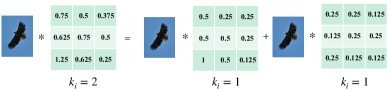
Figure 3. Equivalent conversion from a convolution with a $\mathbf{k}_{i}>1$ filter to $\mathbf{k}_{i}$ convolutions each with a $\mathbf{k}_{i}=1$ filter. This transforms the hardware implementation of the FLightNN into LightNN-1.

4.2. Differentiable training

Instead of picking the threshods $t$ by hand, we consider them as trainable parameters. Therefore, the loss function $\mathcal{L}(\mathbf{w},\mathbf{t})$ is a function of both weights and thresholds. Similar to prior work on DNN quantization (Zhou et al., 2016; Courbariaux et al., [n. d.]), we use the straight-through estimator (STE) (Bengio et al., 2013) to compute $\frac{\partial\mathcal{L}}{\partial\mathbf{w}_{i}}$. By defining $\frac{\partial\mathbf{w}_{i}^{q}}{\partial\mathbf{w}_{i}}=1$ where $\mathbf{w}_{i}^{q}=\mathcal{Q}_{k}(\mathbf{w}_{i}|\mathbf{t})$ is the quantized $\mathbf{w}_{i}$; therefore, we have $\frac{\partial\mathcal{L}}{\partial\mathbf{w}_{i}}=\frac{\partial\mathcal{L}}{\partial\mathbf{w}_{i}^{q}}\cdot\frac{\partial\mathbf{w}_{i}^{q}}{\partial\mathbf{w}_{i}}=\frac{\partial\mathcal{L}}{\partial\mathbf{w}_{i}^{q}}$, which becomes a differentiable expression.

To compute the gradient for thresholds, i.e., $\frac{\partial\mathbf{w}_{i}^{q}}{\partial\mathbf{t}_{j}}$, we relax the indicator function $g(x,\mathbf{t}_{j})=\mathbbm{1}(x>\mathbf{t}_{j})$ to a sigmoid function (Han and Moraga, [n. d.]), $\sigma(.)$, when computing gradients, i.e., $\hat{g}(x,\mathbf{t}_{j})=\sigma(x-\mathbf{t}_{j})$. In addition, we use STE to compute the gradient for $R(x)$. Thus, the gradient $\frac{\partial\mathbf{w}_{i}^{q}}{\partial\mathbf{t}_{j}}$ can be computed by:

$$\begin{split}&\frac{\partial\mathcal{Q}_{\mathbf{k}_{i}}(\mathbf{w}_{i}|\mathbf{t})}{\partial\mathbf{t}_{j}}=\sum_{l=0}^{\mathbf{k}_{i}-1}\frac{\partial\sigma(||\mathbf{r}_{i,l}||_{2}-\mathbf{t}_{l})}{\partial\mathbf{t}_{j}}R(\mathbf{r}_{i,l})+\sigma(||\mathbf{r}_{i,l}||_{2}-\mathbf{t}_{l})\frac{\partial R(\mathbf{r}_{i,l})}{\partial\mathbf{t}_{j}}\\ =&\sum_{l=0}^{\mathbf{k}_{i}-1}\sigma^{\prime}(||\mathbf{r}_{i,l}||_{2}-\mathbf{t}_{l})(\frac{\partial||\mathbf{r}_{i,l}||_{2}}{\partial\mathbf{t}_{j}}-\frac{\partial\mathbf{t}_{l}}{\partial\mathbf{t}_{j}})R(\mathbf{r}_{i,l})+\sigma(||\mathbf{r}_{i,l}||_{2}-\mathbf{t}_{l})\frac{\partial\mathbf{r}_{i,l}}{\partial\mathbf{t}_{j}}\end{split}$$

where $\frac{\partial||\mathbf{r}_{i,l}||_{2}}{\partial\mathbf{t}_{j}}$ and $\frac{\partial\mathbf{r}_{i,l}}{\partial\mathbf{t}_{j}}$ are $0$ for $l<j$; otherwise, they can be computed with the result of $\frac{\partial\mathcal{Q}_{l}(\mathbf{w}_{i}|\mathbf{t})}{\partial\mathbf{t}_{j}}$. $\frac{\partial\mathbf{t}_{l}}{\partial\mathbf{t}_{j}}=\mathbbm{1}(l=j)$.

4.3. Regularization

To encourage smaller $\mathbf{k}_{i}$ for the filters, we also add a regularization loss: $\mathcal{L}_{reg,k}(\mathbf{w})=\sum_{j=0}^{k-1}\lambda_{j}\sum_{i}||\mathbf{r}_{i,j}||_{2}$ where $\lambda_{j}$ performs as a handle to balance accuracy and model sparsity. This regularization loss is the sum of several group Lasso losses, since they can introduce structural sparsity (Wen et al., [n. d.]). The first item $\lambda_{0}\sum_{i}||\mathbf{r}_{i,0}||_{2}=\lambda_{0}\sum_{i}||\mathbf{w}_{i}||_{2}$ is used to prune the whole filters out, while the other items ($j>0$) regularize the residuals. Fig. 4 shows the two items of regularization loss and their sum for the case $k=2$, with $\lambda_{0}$=1e-5 and $\lambda_{1}$=3e-5. Therefore, the total loss for training a FLightNN is: $\mathcal{L}_{total}(\mathbf{w},\mathbf{t})=\mathcal{L}_{CE}(\mathbf{w},\mathbf{t})+\mathcal{L}_{reg,k}(\mathbf{w})$.

The new training algorithm is summarized in Algo. 1. This is the same as the conventional backpropagation algorithm for full-precision DNNs, except that in the forward phase, the weights are quantized given the thresholds $\mathbf{t}$. Then, due to the differentiability of the quantization function w.r.t. $\mathbf{w}$ and $\mathbf{t}$, one can compute their gradients and update their values in each training iteration.

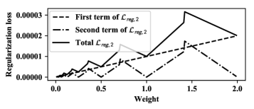
Figure 4. Regularization loss curve $w.r.t.$ weight value.

Input: Training dataset (x, y), where x is input and y is label; parameters after the $(p-1)$-th iteration: ${\textbf{w}}_{p-1}$ (weights), ${\textbf{b}}_{p-1}$ (biases), and quantization thresholds ${\textbf{t}}_{p-1}$; quantization function $\mathcal{Q}_{k}({\textbf{w}}|{\textbf{t}})$; DNN forward computation function $g(x,w,b)$; maximum k value used for all filters; regularization loss coefficients $\lambda$; learning rate $\eta$.

Output: Updated weights ${\textbf{w}}_{p}$, biases ${\textbf{b}}_{p}$ and thresholds ${\textbf{b}}_{p}$.

for each mini-batch of x, y do

       1. Quantize weights: ${\textbf{w}}^{q}=\mathcal{Q}_{k}({\textbf{w}}_{p-1}|{\textbf{t}}_{p-1})$

       2. Forward: compute intermediate results and cross entropy loss function $\mathcal{L}_{CE}$ with $g(\cdot)$, ${\textbf{w}}^{q}$, ${\textbf{b}}_{p-1}$, and mini-batch of x; compute regularization loss $\mathcal{L}_{reg,k}$ with $\lambda$ and ${\textbf{w}}_{p-1}$; get the total loss $\mathcal{L}_{total}=\mathcal{L}_{CE}+\mathcal{L}_{reg,k}$

       3. Backward: compute derivatives $\frac{\partial\mathcal{L}_{total}}{\partial{\textbf{w}}^{q}}$, $\frac{\partial\mathcal{L}_{total}}{\partial{\textbf{b}}_{p-1}}$, and $\frac{\partial\mathcal{L}_{total}}{\partial{\textbf{t}}_{p-1}}$

       4. Update parameters: ${\textbf{w}}_{p}={\textbf{w}}_{p-1}-\eta\frac{\partial\mathcal{L}_{total}}{\partial{\textbf{w}}^{q}}$; ${\textbf{b}}_{p}={\textbf{b}}_{p-1}-\eta\frac{\partial\mathcal{L}_{total}}{\partial{\textbf{b}}_{p-1}}$; ${\textbf{t}}_{p}={\textbf{t}}_{p-1}-\eta\frac{\partial\mathcal{L}_{total}}{\partial{\textbf{t}}_{p-1}}$

      

end for

Algorithm 1 FLightNN Training Epoch

5. Experimental Results

In this section, we first introduce the experiment setup. Then, we show the accuracy results of different quantized DNN models by software training, as well as their throughput on the FPGA and energy efficiency on the ASIC, to verify the effectiveness of FLightNNs.

5.1. Setup

We conduct experiments on both small and large CNNs for CIFAR-10, SVHN, CIFAR-100 and ImageNet datasets. The eight adopted network configurations are shown in Table 1. To explore the FLightNN performance on different types of network structures, we use a VGG structure with a series of stacked convolutional layers for Network 1, 3, 4 and 5, and adopt the ResNet structure with skip connections across layers for network 2, 6, 7 and 8. Networks 1, 2 and 3 are used for experiments on CIFAR-10; networks 4 and 5 are used for SVHN; networks 6 and 7 are used for CIFAR-100; the last one, network 8, is used for ImageNet. For all networks, each convolutional layer is followed by a batch normalization layer and a Leaky ReLU activation function (Maas et al., [n. d.]), and optionally followed by a max-pooling layer. We use the Adam optimizer (Kingma and Ba, 2015) to train the network. For each of the networks, we train different quantized models including full-precision DNNs, fixed-point DNNs with 4-bit weights and 8-bit activations, LightNN-2 with 8-bit weights and 8-bit activations, LightNN-1 with 4-bit weights and 8-bit activations, and FLightNNs with 8-bit activations. Due to large training times and limitations in computing resources, we train the ImageNet dataset on a ResNet-10 with reduced width (i.e., network 8), for LightNN-1, LightNN-2 and FLightNNs. For all FLightNNs, we initialize the threshods $\mathbf{t}$ to $\mathbf{0}$, and set the largest shifts $k$ as 2. For all, except the 32-bit full-precision model, we use 8-bit fixed-point quantization for the activations. By varying $\lambda$, we can have different accuracy-throughput or accuracy-energy trade-offs for FLightNNs. All these networks are trained in software through PyTorch.

Table 1. Network settings. “Depth” is the number of convolutional layers in the network. “Width” is the number of convolutional filters of the largest layer.

Network ID	Parameters	Structure	Depth	Width
1	0.08M	VGG	7	64
2	0.7M	ResNet	18	128
3	4.6M	VGG	7	512
4	0.03M	VGG	4	64
5	0.1M	VGG	4	128
6	0.7M	ResNet	18	128
7	2.8M	ResNet	18	256
8	1.8M	ResNet	10	256

5.2. Accuracy-throughput trade-off on FPGA

To show the accuracy-throughput trade-off of the models, we implement the inference of each network’s largest convolutional layer for each of the quantized DNN models on FPGA since prior work has shown that convolution operations typically take over 90% of the computation time of a CNN (Zhang et al., [n. d.]). Our implementation is built on the Xilinx Zynq ZC706 evaluation board. Its working frequency is 100 MHz. Pre-synthesis is executed on an Intel i7-4790 CPU (3.6GHz) with 16GB RAM. We use Vivado HLS (Xilinx, 2017) for FPGA implementation. The C code of DNN designs are parallelized by adding HLS-defined pragma and the parallel version is validated with the Vivado HLS timing analysis tool. To make a fair comparison, the same pragma and directives are used for full-precision, fixed-point DNNs, LightNNs and FLightNNs, and we follow the same scheduling settings as prior work (Ding et al., 2018). Batched inference is adopted, and the maximum batch size without running out of FPGA resources is set to obtain the highest throughtput.

Tables 2, 3, 4 and 5 show the accuracy and throughput comparison for full-precision DNNs, fixedpoint DNNs, LightNNs and FLightNNs. For all the experimented datasets, LightNNs show the advantage of flexible accuracy-speed trade-offs. In most of the networks (e.g., networks 1, 3, 6 and 7), FLightNNs can achieve an accuracy close to LightNN-2, but have much higher speedup than LightNN-2. Thus, FLightNNs provide continuous trade-offs for accuracy and speed. Compared to the fixed-point quantization, FLightNNs can achieve higher accuracy, and up to $2.0\times$, $1.8\times$ and $1.8\times$ speedup for CIFAR-10, SVHN, CIFAR-100 datasets, respectively. This is because the multiplication is replaced by shift operators, which require only LUT resources on FPGA while the multipliers require DSP units which are generally more scarce than LUT. Therefore, the computation for FLightNNs allows larger batch sizes than that of fixed-point DNNs, increasing data parallelism, and thus, improving the throughput.

It is also interesting to note that by comparing some FLightNNs (e.g., FL_1a, FL_2a, FL_3a, FL_6a and FL_7a) with LightNN-1, we find that FLightNNs can achieve higher accuracy with the same or even lower storage as LightNN-1. This is because initially FLightNNs quantize all the filters with two shifts (since $\mathbf{t}$ is initialized as $\mathbf{0}$), and gradually add constraints to the filters. This gradual quantization may be better than training a network with only one shift from scratch, as LightNN-1 does. The benefit of gradual quantization has also been observed by prior work (Dong et al., 2017) which shows that gradually imposing quantization constraints can achieve better accuracy than directly quantizing with a strict constraint.

Table 6 shows the FPGA resources utilization for networks 7 and 8. Since full-precision and fixed-point DNNs require DSP for both multiplication and addition, while LightNNs and FLightNNs only need DSP for addition, full-precision and fixed-point DNNs have larger DSP resource utilization. Compared to full-precision DNNs which use 32-bit floating point operations, fixed-point DNNs only use 4-bit weights and 8-bit activations, and therefore consume fewer DSP units. LightNNs and FLightNNs use LUT to implement the multipliers, and have a higher utilization of LUT than full-precision and fixed-point DNNs. However, the performance of (F)LightNNs is not bounded by LUT resources since the maximum usage of LUT by LightNN-2 is only 42% and 17% for networks 7 and 8, respectively. Instead, the memory resource (BRAM) bounds the performance for (F)LightNNs, while for full-precision and fixed-point DNNs, the performance is bounded by both BRAM and DSP.

Table 2. Accuracy and FPGA throughput for CIFAR-10. In the “Model” column, “Full”, “L-2”, “L-1”, “FP”, “FL” indicate full-precision DNN, LightNN-2, LightNN-1, Fixed-point DNN, and FLightNN, respectively. The subscript “$x$W$y$A” indicates $x$ bits for weights and $y$ bits for activations. The FLightNN results are shown in bold face. We use subscript $a$ and $b$ to denote the two trained FLightNNs for each network. These notations also apply for Table 3, 4 and 5.

ID	Model	Accuracy (%)	Storage (MB)	Throughput (images/s)	Speedup
1	Full	86.36	0.31	3.2e2	1$\times$
	L-28W8A	86.17	0.08	2.2e3	7.0$\times$
	L-14W8A	84.82	0.04	4.5e3	14.4$\times$
	FP4W8A	85.09	0.04	3.3e3	10.5$\times$
	FL1a	85.70	0.04	4.8e3	15.0$\times$
	FL1b	85.91	0.06	4.0e3	12.6$\times$
2	Full	91.70	2.8	1.4e2	1$\times$
	L-28W8A	91.64	0.7	1.6e3	11.5$\times$
	L-14W8A	91.15	0.4	2.7e3	19.0$\times$
	FP4W8A	91.17	0.4	1.5e3	10.7$\times$
	FL2a	91.36	0.4	2.8e3	18.9$\times$
	FL2b	91.48	0.7	1.9e3	13.0$\times$
3	Full	92.85	18.5	1.3	1$\times$
	L-28W8A	92.72	4.6	10.2	7.8$\times$
	L-14W8A	91.93	2.3	39.2	30.2$\times$
	FP4W8A	92.23	2.3	19.8	15.2$\times$
	FL3a	92.59	2.3	39.2	30.2$\times$
	FL3b	92.62	3.3	27.2	21.0$\times$

Table 3. Accuracy and FPGA throughput for SVHN.

ID	Model	Accuracy (%)	Storage (MB)	Throughput (images/s)	Speedup
4	Full	94.96	0.12	2.2e3	1$\times$
	L-28W8A	94.90	0.03	4.5e3	2.09$\times$
	L-14W8A	94.16	0.02	8.3e3	3.63$\times$
	FP4W8A	93.70	0.02	3.7e3	1.70$\times$
	FL4a	94.67	0.02	6.7e3	3.11$\times$
	FL4b	94.88	0.03	5.3e3	2.37$\times$
5	Full	96.44	0.4	1.1e3	1$\times$
	L-28W8A	96.38	0.1	2.1e3	2.00$\times$
	L-14W8A	95.93	0.05	3.7e3	3.53$\times$
	FP4W8A	96.02	0.05	1.8e3	1.71$\times$
	FL5a	96.21	0.06	3.2e3	3.06$\times$
	FL5b	96.24	0.08	3.0e3	2.84$\times$

Table 4. Accuracy and FPGA throughput for CIFAR-100.

ID	Model	Accuracy (%)	Storage (MB)	Throughput (images/s)	Speedup
6	Full	69.16	2.8	2.5e2	1$\times$
	L-28W8A	68.84	0.7	1.6e3	6.4$\times$
	L-14W8A	67.32	0.4	2.7e3	10.6$\times$
	FP4W8A	67.67	0.4	1.5e3	5.98$\times$
	FL6a	68.59	0.4	2.7e3	10.6$\times$
	FL6b	68.76	0.6	1.8e3	6.88$\times$
7	Full	71.22	11.2	7.4e1	1$\times$
	L-28W8A	70.96	2.8	6.0e2	8.11$\times$
	L-14W8A	69.71	1.4	1.1e3	15.2$\times$
	FP4W8A	69.34	1.4	6.9e2	9.26$\times$
	FL7a	70.85	1.4	1.1e3	15.2$\times$
	FL7b	70.87	2.4	7.4e2	9.98$\times$

Table 5. Top-5 Accuracy and FPGA throughput for ImageNet.

ID	Model	Accuracy (%)	Storage (MB)	Throughput (images/s)	Speedup
8	L-28W8A	75.04	1.8	2.7e2	1$\times$
	L-14W8A	72.94	0.9	5.2e2	1.95$\times$
	FL8a	74.80	1.5	3.1e2	1.16$\times$
	FL8b	75.00	1.7	2.8e2	1.06$\times$

Table 6. FPGA resource utilization for different quantized DNN models.

ID	Model	Maximum resource utilization				Speedup
		BRAM	DSP	FF	LUT
7	Full	896	642	69,344	128,339	1$\times$
	L-28W8A	1,024	4	66,491	90,949	8.11$\times$
	L-14W8A	1,024	4	66,491	90,949	15.2$\times$
	FP4W8A	1,024	514	7,110	90,949	9.26$\times$
	FL7a	1,024	4	84,192	90,949	9.98$\times$
	FL7b	1,024	4	63,648	80,940	15.2$\times$
8	L-28W8A	832	16	3,156	38,022	1$\times$
	L-18W8A	800	16	3,084	36,906	1.95$\times$
	FL8a	800	16	5,070	36,098	1.16$\times$
	FL8b	800	16	6,272	37,406	1.06$\times$
Available		1,090	900	437,200	218,600

5.3. Accuracy-energy trade-off on ASIC

For all quantized DNNs, we designed pipelined implementations with one stage per neuron, where the computation unit is reused for each neuron. A 65nm commercial standard library is adopted. The Synopsys Design Compiler (Manual, 2010) is used to generate the gate-level netlist of the computation units. The power consumption of all computation operations within one layer is calculated using Synopsys Primetime. We keep all the DNN architectures implemented in an unoptimized fashion because our main objective is to compare how different quantized DNNs impact computational energy.

The accuracy and computational energy trade-offs for the quantized DNN models are shown in Fig. 5. The energy shown in Fig. 5 only includes the computational energy consumption for the largest layer of each network. We can clearly observe that FLightNNs provide a more continuous Pareto front for LightNN-2 and LightNN-1, regardless of the network type (i.e., VGG or ResNet), size and the datasets. Similar to the observation in Sec. 5.2, in some networks FLightNNs can achieve higher accuracy than LightNN-1 with lower computational energy cost.

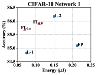
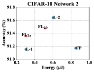
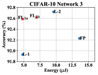
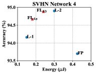
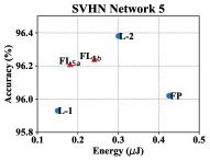
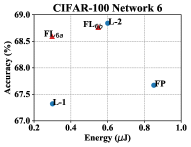
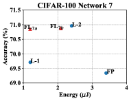
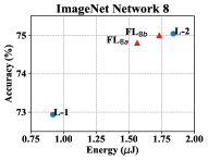
Figure 5. Accuracy and computational energy consumption in ASIC for different quantized models on CIFAR-10, SVHN, CIFAR-100 and ImageNet datasets. FLightNNs are marked as red triangles, while the other models are shown as blue dots.

6. Discussion

Since FLightNNs customize the $\mathbf{k}_{i}$ for each filter, LightNN-1 and LightNN-2 can be considered as two special cases for FLightNNs. Therefore, the Pareto front created by the searched FLightNN solutions should be the upper bound for the front of LightNN-1 and LightNN-2 with varied parameter numbers. We test this hypothesis on CIFAR-100 dataset using networks with varied number of convolutional filters. As shown in Fig. 6, the accuracy-storage Pareto-front created by FLightNNs is consistently higher than the LightNNs. This indicates that instead of only filling in the Pareto front of LightNNs, FLightNNs can push forward the Pareto front, due to their larger design space. The proposed differentiable training algorithm optimizes both $\mathbf{k}_{i}$ and weight values in an end-to-end fashion, and therefore significantly reduces searching effort compared to exhaustive or heuristic methods with multiple rounds of training. Future work will further improve training efficiency by using optimized training loss (Ding et al., 2019) or proper labels (Chen et al., 2018).

7. Conclusion

In this paper, we propose FLightNNs which customize the number of shift operations for each filter of LightNNs. Equipped with the proposed differentiable training algorithm, FLightNNs can achieve a flexible trade-off between accuracy and speed/energy. Our experimental results on FPGA and ASIC simulations show that FLightNNs can provide a more continuous Pareto front for LightNN models and consistently outperform fixed-point DNNs w.r.t. both accuracy and speed/energy. Moreover, due to the gradual quantization nature of the differentiable training, FLightNNs can achieve higher accuracy than LightNN-1 without sacrificing speed and energy efficiency, and thus, push forward the Pareto-optimal front. These promising results suggest the potentials for FLightNNs to achieve fast and accurate inference on learning-based customized hardware.

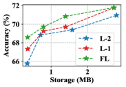
Figure 6. Accuracy-storage front for LightNN-2 LightNN-1 and FLightNN. The Pareto front of FLightNN is the upper bound of LightNNs.

- (1)
- NNA ([n. d.]) [n. d.]. NNAPI. https://developer.android.com/ndk/guides/neuralnetworks/. Accessed: 2018-10-15.
- Bengio et al. (2013) Yoshua Bengio, Nicholas Léonard, and Aaron Courville. 2013. Estimating or propagating gradients through stochastic neurons for conditional computation. arXiv preprint arXiv:1308.3432 (2013).
- Brooks ([n. d.]) David M Brooks. [n. d.]. Co-designed Systems for Deep Learning Hardware Accelerators. In IEEE VLSI Design, Automation and Test (VLSI-DAT), International Symposium. 1–1, 2018.
- Chen et al. ([n. d.]) Yu-Hsin Chen, Tushar Krishna, Joel S Emer, and Vivienne Sze. [n. d.]. Eyeriss: An Energy-efficient Reconfigurable Accelerator for Deep Convolutional Neural Networks. IEEE Journal of Solid-State Circuits 52, 1 ([n. d.]), 127–138, 2017.
- Chen et al. (2018) Zhuo Chen, Ruizhou Ding, Ting-Wu Chin, and Diana Marculescu. 2018. Understanding the Impact of Label Granularity on CNN-based Image Classification. In 2018 IEEE International Conference on Data Mining Workshops (ICDMW). IEEE, 895–904.
- Courbariaux et al. ([n. d.]) Matthieu Courbariaux, Yoshua Bengio, and Jean-Pierre David. [n. d.]. Binaryconnect: Training deep neural networks with binary weights during propagations. In Advances in neural information processing systems. 3123–3131, 2015.
- Ding et al. (2019) Ruizhou Ding, Ting-Wu Chin, Diana Marculescu, and Zeye Liu. 2019. Regularizing Activation Distribution for Training Binarized Deep Networks. In IEEE CVPR. IEEE.
- Ding et al. (2018) Ruizhou Ding, Zeye Liu, RD Blanton, and Diana Marculescu. 2018. Lightening the Load with Highly Accurate Storage- and Energy-Efficient LightNNs. ACM transactions on Reconfigurable Technology and Systems 11, 3 (2018), 20–44.
- Ding et al. (2017) Ruizhou Ding, Zeye Liu, Rongye Shi, Diana Marculescu, and RD Blanton. 2017. LightNN: Filling the Gap between Conventional Deep Neural Networks and Binarized Networks. In Proceedings of the on Great Lakes Symposium on VLSI. ACM, 35–40, 2017.
- Dong et al. (2017) Yinpeng Dong, Renkun Ni, Jianguo Li, Yurong Chen, Jun Zhu, and Hang Su. 2017. Learning Accurate Low-Bit Deep Neural Networks with Stochastic Quantization. BMVC (2017).
- Gupta et al. ([n. d.]) Suyog Gupta, Ankur Agrawal, Kailash Gopalakrishnan, and Pritish Narayanan. [n. d.]. Deep learning with limited numerical precision. In Proceedings of the 32nd International Conference on Machine Learning. 1737–1746, 2015.
- Han and Moraga ([n. d.]) Jun Han and Claudio Moraga. [n. d.]. The influence of the sigmoid function parameters on the speed of backpropagation learning. In International Workshop on Artificial Neural Networks. 195–201, 1995.
- Han et al. ([n. d.]) Song Han, Jeff Pool, John Tran, and William Dally. [n. d.]. Learning Both Weights and Connections for Efficient Neural Network. In Advances in Neural Information Processing Systems. 1135–1143, 2015.
- Hubara et al. (2016) Itay Hubara, Matthieu Courbariaux, Daniel Soudry, Ran El-Yaniv, and Yoshua Bengio. 2016. Binarized Neural Networks. In Advances in Neural Information Processing Systems. 4107–4115, 2016.
- Kingma and Ba (2015) Diederik P Kingma and Jimmy Ba. 2015. Adam: A method for stochastic optimization. ICLR (2015).
- Lin et al. (2016) Darryl Lin, Sachin Talathi, Sachin Talathi, and Sreekanth Annapureddy. 2016. Fixed point quantization of deep convolutional networks. In International Conference on Machine Learning. 2849–2858, 2016.
- Liu et al. (2018) Hanxiao Liu, Karen Simonyan, and Yiming Yang. 2018. Darts: Differentiable architecture search. arXiv preprint arXiv:1806.09055 (2018).
- Louizos et al. (2018) Christos Louizos, Max Welling, and Diederik P. Kingma. 2018. Learning Sparse Neural Networks through L_0 Regularization. In International Conference on Learning Representations.
- Maas et al. ([n. d.]) Andrew L Maas, Awni Y Hannun, and Andrew Y Ng. [n. d.]. Rectifier nonlinearities improve neural network acoustic models. In Proc. ICML, Vol. 30. 3, 2013.
- Manual (2010) Synopsys MEDICI User’s Manual. 2010. Synopsys inc. Mountain View, CA (2010).
- Marculescu et al. (2018) Diana Marculescu, Dimitrios Stamoulis, and Ermao Cai. 2018. Hardware-aware machine learning: modeling and optimization. In Proceedings of the International Conference on Computer-Aided Design. ACM, 137.
- Sandler et al. ([n. d.]) Mark Sandler, Andrew Howard, Menglong Zhu, Andrey Zhmoginov, and Liang-Chieh Chen. [n. d.]. MobileNetV2: Inverted Residuals and Linear Bottlenecks. In Proceedings of the IEEE Conference on Computer Vision and Pattern Recognition. 4510–4520, 2018.
- Stamoulis et al. (2018a) Dimitrios Stamoulis, Ermao Cai, Da-Cheng Juan, and Diana Marculescu. 2018a. HyperPower: Power-and memory-constrained hyper-parameter optimization for neural networks. In 2018 Design, Automation & Test in Europe Conference & Exhibition (DATE). IEEE, 19–24.
- Stamoulis et al. (2018b) Dimitrios Stamoulis, Ting-Wu Rudy Chin, Anand Krishnan Prakash, Haocheng Fang, Sribhuvan Sajja, Mitchell Bognar, and Diana Marculescu. 2018b. Designing adaptive neural networks for energy-constrained image classification. In Proceedings of the International Conference on Computer-Aided Design. ACM, 23.
- Tann et al. ([n. d.]) Hokchhay Tann, Soheil Hashemi, R Iris Bahar, and Sherief Reda. [n. d.]. Hardware-software Codesign of Accurate, Multiplier-free Deep Neural Networks. In 54th Design Automation Conference (DAC). 1–6, 2017.
- Wen et al. ([n. d.]) Wei Wen, Chunpeng Wu, Yandan Wang, Yiran Chen, and Hai Li. [n. d.]. Learning Structured Sparsity in Deep Neural Networks. In Advances in Neural Information Processing Systems. 2074–2082, 2016.
- Xilinx (2017) Xilinx. 2017. Vivado High-Level Synthesis. https://www.xilinx.com/products/design-tools/vivado/integration/esl-design.html (2017).
- Yang et al. ([n. d.]) Tien-Ju Yang, Yu-Hsin Chen, and Vivienne Sze. [n. d.]. Designing Energy-Efficient Convolutional Neural Networks Using Energy-Aware Pruning. In IEEE CVPR. 6071–6079, 2017.
- Zhang et al. ([n. d.]) Chen Zhang, Peng Li, Guanyu Sun, Yijin Guan, Bingjun Xiao, and Jason Cong. [n. d.]. Optimizing FPGA-based Accelerator Design for Deep Convolutional Neural Networks. In Proceedings of the International Symposium on Field-Programmable Gate Arrays. 161–170, 2015.
- Zhao and Liu (2018) Hengyu Zhao and Jiawen Liu. 2018. Processing-in-Memory for Energy-efficient Neural Network Training: A Heterogeneous Approach. In IEEE/ACM International Symposium on Microarchitecture.
- Zhou et al. (2016) Shuchang Zhou, Yuxin Wu, Zekun Ni, Xinyu Zhou, He Wen, and Yuheng Zou. 2016. Dorefa-net: Training low bitwidth convolutional neural networks with low bitwidth gradients. arXiv preprint arXiv:1606.06160 (2016).