Helicoidal excitonic phase in an electron-hole double layer system

Abstract

We propose helicoidal excitonic phase in a Coulomb-coupled two-dimensional electron-hole double layer (EHDL) system with relativistic spin-orbit interaction. Previously, it was demonstrated that layered InAs/AlSb/GaInSb heterostructure is an ideal experimental platform for searching excitonic condensate phases, while its electron layer has non-negligible Rashba interaction. We clarify that due to the Rashba term, the spin-triplet (spin-1) exciton field in the EHDL system forms a helicoidal structure and the helicoid plane can be controlled by an in-plane Zeeman field. We show that due to small but finite Dirac term in the heavy hole layer the helicoidal structure of the excitonic field under the in-plane field results in a helicoidal magnetic order in the electron layer. Based on linearization analyses, we further calculate momentum-energy dispersions of low-energy Goldstone modes in the helicoidal excitonic phase. We discuss possible experimental probes of the excitonic phase in the EHDL system.

I introduction

One of the fundamental challenges in condensed matter physics is an experimental realization of excitonic condensation and excitonic insulator at the equilibrium mott61 ; knox63 ; keldysh65 ; jerome67 ; halperin68 ; wakisaka09 ; kogar17 ; werdehausen18 . Early experiments report significant electron-hole Coulomb drag phenomena in bilayer quantum well structure lozovik75 ; comte82 ; datta85 ; xia92 ; zhu95 ; littlewood96 ; naveh96 made out of semiconductors such as GaAs/AlGaAs croxall08 ; seamons09 ; yang11 or Si sivan92 . Recently, a strained layer InAs/AlSb/GaInSb heterostructure naveh96 ; wu19 provides an ideal platform of Coulomb coupled electron-hole double layer (EHDL) system, that has a lot of advantages over the others. Thereby, a dual gate device enables a continuous change of both chemical potential and charge state energy. Large relativistic spin-orbit interaction (SOI) realizes a nearly isotropic Fermi contour of the heavy hole band as well as the electron band. In fact, a recent experiment reports a transport signature of the excitonic coupling in the charge neutrality regime of the strained layer heterostructure wu19 .

The excitonic pairing in Coulomb coupled EHDL system is either of the spin triplet (spin-1) nature or of the spin-singlet (spin-0) nature zhu95 ; zhu96 . An energy degeneracy between these two will be lifted by the large SOI in the electron layer of the EHDL system. Besides, due to the SOI, the spin triplet vector (spin-1 vector) could exhibit a non-trivial spatial texture, that breaks the translational symmetry in the two-dimensional plane. The spatial texture of the excitonic pairing field in EHDL system is generally free from charged and/or magnetic impurities in each layer, while it could be pinned by a spatial variation of the dielectric constant in the intermediate separation layer. To our best knowledge, it is entirely an open question at this moment how the spin-1 exciton forms spatial textures in the presence of the SOI, how the textures could be coupled with external magnetic (Zeeman) field, what kind of low-energy collective excitations would emerge from the translational symmetry breaking, and how the texture could be experimentally detected.

In this paper, we identify the spatial textures of the spin-1 exciton condensate in the presence of the SOI, clarify the natures of the low-energy collective modes in the excitonic phase, and propose possible experimental probes for detecting the spatial texture of the spin-1 exciton condensate. First, we derive a $\phi^{4}$ effective action for the spin-triplet (spin-1) excitonic pairing field and determine a form of the couplings among the exciton, the SOI and the magnetic Zeeman field. We then propose that helicoidal structures of the spin-1 exciton minimize the classical action. Based on the effective action and the classical configuration, we derive linearized EOMs for fluctuations of the spin triplet exciton field around the classical configuration. From the EOMs, we calculate the low-energy collective excitations in the helicoidal excitonic condensate. Using these theoretical knowledges, we propose possible experimental probes for detecting the helicoidal excitonic texture in the EHDL system.

II model and effective action

We begin with a non-interacting Hamiltonian for the two-dimensional EHDL system pikulin14 ;

$$H_{0}-\mu N \equiv\int d{\bm{x}}\!\ {\bm{a}}^{\dagger}({\bm{x}})\bigg{[}\Big{(}-\frac{\hbar^{2}\nabla^{2}}{2m_{e}}-E_{g}-\mu\Big{)}{\bm{\sigma}}_{0}$$

$$\ \ \ +\xi_{e}\big{(}-i\partial_{y}{\bm{\sigma}}_{x}+i\partial_{x}{\bm{\sigma}}_{y}\Big{)}+H{\bm{\sigma}}_{H}\bigg{]}{\bm{a}}({\bm{x}})$$

$$+\int d{\bm{x}}\!\ {\bm{b}}^{\dagger}({\bm{x}})\bigg{[}\Big{(}\frac{\hbar^{2}\nabla^{2}}{2m_{h}}+E_{g}-\mu\Big{)}{\bm{\sigma}}_{0}$$

$$\ +\Delta_{h}\big{(}-i\partial_{x}{\bm{\sigma}}_{x}-i\partial_{y}{\bm{\sigma}}_{y}\Big{)}+H{\bm{\sigma}}_{H}\bigg{]}{\bm{b}}({\bm{x}}),$$ (1)

with $H=x,y$, ${\bm{x}}\equiv(x,y)$, ${\bm{\sigma}}_{0}$, and ${\bm{\sigma}}_{i}$ ($i=x,y,z$) are two by two unit and Pauli matrices. ${\bm{a}}^{\dagger}({\bm{x}})\equiv(a^{\dagger}_{\uparrow}({\bm{x}}),a^{\dagger}_{\downarrow}({\bm{x}}))$ and ${\bm{b}}^{\dagger}({\bm{x}})\equiv(b^{\dagger}_{\uparrow}({\bm{x}}),b^{\dagger}_{\downarrow}({\bm{x}}))$ denote the creation and annihilation operators of electron and hole bands with respective mass $m_{e}\!\ (>0)$ and $m_{h}\!\ (>0)$. The chemical potential $\mu$ as well as the charge state energy $E_{g}$ (band inversion parameter) can be separately tuned by the dual gate device. The SOI in the electron band with $S_{z}=\pm 1/2$ doublet takes a form of the Rashba term with $\xi_{e}$ and the SOI in the heavy hole band with $J_{z}=\pm 3/2$ doublet takes a form of the Dirac term with $\Delta_{h}$. In the InAs/AlSb/GaInSb heterostructure, the Rashba term in the electron layer is much larger than that in the heavy hole band; $\xi_{e}/(E_{0}d_{0})\sim-0.1$, $\Delta_{h}/(E_{0}d_{0})\sim 0.001$, Here $E_{0}$ and $d_{0}$ (thickness of the intermediate separation layer) define a length scale and energy scale of the EHDL system; $E_{0}=(m^{-1}_{e}+m^{-1}_{h})\hbar^{2}/2d^{2}_{0}=e^{2}/(4\pi\epsilon\epsilon_{0}d_{0})$. Typically, $E_{0}/k_{\rm B}=100$K and $d_{0}=10$ nm pikulin14 ; wu19 . For simplicity, we take $\Delta_{h}=0$, unless dictated otherwise (e.g. Section. V). To study how the spatial texture of the spin-1 exciton condenate can be changed by an in-plane magnetic field, we include the magnetic Zeeman field $H$ along the in-plane direction ($H=x,y$).

The electron and hole layers are coupled with each other through the long-range Coulomb interaction. For simplicity, we employ the short-ranged repulsive interaction;

$$H_{\rm int}=g\int d{\bm{x}}\!\ a^{\dagger}_{\sigma}({\bm{x}})a_{\sigma}({\bm{x}})\!\ b^{\dagger}_{\sigma^{\prime}}({\bm{x}})b_{\sigma^{\prime}}({\bm{x}}).$$ (2)

with $g>0$. The spin-rotational symmetry in Eq. (2) allows to decompose the interaction into the spin singlet and triplet parts. In terms of the respective excitonic pairing fields $\hat{\cal O}_{\mu}({\bm{x}})\equiv{\bm{a}}^{\dagger}({\bm{x}}){\bm{\sigma}}_{\mu}{\bm{b}}({\bm{x}})$ ($\mu=0,x,y,z$), the interaction part takes a form of

$$H_{\rm int}=-\frac{g}{2}\int d{\bm{x}}\!\ \sum_{\mu=0,x,y,z}\hat{\cal O}^{\dagger}_{\mu}({\bm{x}})\hat{\cal O}_{\mu}({\bm{x}}).$$ (3)

Using the Stratonovich-Hubbard transformation followed by a standard procedure (appendix A), we derive a partition function $Z$ and its action $S$, that is a functional of the spin-triplet (spin-1) exciton pairing fields (‘$g$-vector’); $\phi_{\mu}({\bm{x}})\equiv\frac{g}{2}\langle\hat{\cal O}_{\mu}({\bm{x}})\rangle$ $(\mu=x,y,z)$,

$$Z =\int{\cal D}{\bm{\phi}}^{\dagger}{\cal D}{\bm{\phi}}\!\ \exp\Big{[}-S[{\bm{\phi}}^{\dagger},{\bm{\phi}}]\Big{]}$$

$$S =\int^{\beta}_{0}d\tau\int d{\bm{x}}\bigg{\{}-\eta{\bm{\phi}}^{\dagger}\partial_{\tau}{\bm{\phi}}-\Big{(}\alpha-\frac{2}{g}\Big{)}|{\bm{\phi}}|^{2}+\lambda|{\bm{\nabla}}{\bm{\phi}}|^{2}$$

$$\ \ -\gamma\Big{(}\big{(}|{\bm{\phi}}|^{2}\big{)}^{2}+4\big{(}|{\bm{\phi}}^{\prime}|^{2}|{\bm{\phi}}^{\prime\prime}|^{2}-({\bm{\phi}}^{\prime}\cdot{\bm{\phi}}^{\prime\prime})^{2}\big{)}\Big{)}$$

$$\ \ -D\Big{(}{\bm{e}}_{y}\cdot\big{(}{\bm{\phi}}^{\prime}\times\partial_{x}{\bm{\phi}}^{\prime}\big{)}-{\bm{e}}_{x}\cdot\big{(}{\bm{\phi}}^{\prime}\times\partial_{y}{\bm{\phi}}^{\prime}\big{)}\Big{)}$$

$$\ \ -D\Big{(}{\bm{e}}_{y}\cdot\big{(}{\bm{\phi}}^{\prime\prime}\times\partial_{x}{\bm{\phi}}^{\prime\prime}\big{)}-{\bm{e}}_{x}\cdot\big{(}{\bm{\phi}}^{\prime\prime}\times\partial_{y}{\bm{\phi}}^{\prime\prime}\big{)}\Big{)}$$

$$\ \ -2h{\bm{e}}_{H}\cdot\big{(}{\bm{\phi}}^{\prime}\times{\bm{\phi}}^{\prime\prime}\big{)}\bigg{\}}+{\cal O}(\xi^{2}_{e},H^{2},\xi_{e}H),$$ (4)

with $H=x,y$. ${\bm{e}}_{x}$ and ${\bm{e}}_{y}$ are the unit vectors along $x$ and $y$ axis. $\alpha$ and $\lambda$ are positive, and $\eta$ and $\gamma$ are negative (appendix A). Since $D$ and $h$ are proportional to $\xi_{e}$ and $H$ respectively, we can always assume $D>0$ and $h>0$ without loss of generality. Note that the spin-1 exciton field ${\bm{\phi}}({\bm{x}})$ has both real and imaginary parts, ${\bm{\phi}}^{\prime}({\bm{x}})$ and ${\bm{\phi}}^{\prime\prime}({\bm{x}})$; $\phi_{\nu}({\bm{x}})\equiv\phi^{\prime}_{\nu}({\bm{x}})+i\phi^{\prime\prime}_{\nu}({\bm{x}})$, $\phi^{\dagger}_{\nu}({\bm{x}})\equiv\phi^{\prime}_{\nu}({\bm{x}})-i\phi^{\prime\prime}_{\nu}({\bm{x}})$ ($\mu=x,y,z$). Note also that using a Talyor expansion, we took into account the lowest order in $\xi_{e}$ and $H$. Within the lowest order, the SOI favors helicoid orders of both the real and imaginary parts of the $g$-vector, where a rotational plane of the $g$-vector is parallel to a propagating direction within the $xy$ plane. The Zeeman field is linearly coupled with a vector chirality formed by the real and imaginary parts of the $g$-vector.

The quadratic part of the action in Eq. (4) gives energy dispersions of the spin-1 exciton bands as a function of momentum ${\bm{k}}$. The bands are triply degenerate at the zero momentum point at the zero magnetic field ($h=0$), while the degeneracy is lifted at non-zero momentum due to the SOI term yu14 . In the zero field, the lowest spin triplet exciton band has a ‘wine-bottle’ minimum at a line (ring) of $|{\bm{k}}|=K\equiv D/2\lambda$. The energy at the minimum is $-\alpha+2/g-D^{2}/4\lambda$. When the energy minimum decreases on lowering temperature or on decreasing the charge state energy $E_{g}$, the minimum eventually touches the zero energy. Thereby, the system picks up one ${\bm{k}}$ from the line of $|{\bm{k}}|=K$, and undergoes Bose-Einstein condensation (BEC) pethick01 of the spin-1 exciton band. The resulting phase is what we call in this paper helicoidal excitonic condensate phase. In the next section, we assume that $\alpha-2/g+D^{2}/4\lambda>0$ and describe this helicoidal excitonic phase in details and explain especially how the helicoidal excitonic condensate can be controlled by the in-plane Zeeman field ($h=x,y$).

III helicoidal excitonic condensate

The classical action at the zero magnetic field is maximally minimized by a helicoidal structure of the triplet pairing field;

$${\bm{\phi}}_{c}({\bm{x}})=\rho e^{i\theta}\big{\{}\hat{\bm{k}}\cos({\bm{k}}{\bm{x}})-\hat{e}_{z}\sin({\bm{k}}{\bm{x}})\big{\}},$$ (5)

with

$${\bm{k}} \equiv K\hat{\bm{k}}=\frac{D}{2\lambda}\big{(}\cos\omega\!\ \hat{\bm{e}}_{x}+\sin\omega\!\ \hat{\bm{e}}_{y}\big{)},$$ (6)

$$K \equiv\frac{D}{2\lambda},\ \rho\equiv\sqrt{\frac{1}{2|\gamma|}\Big{(}\alpha-\frac{2}{g}+\frac{D^{2}}{4\lambda}\Big{)}}.$$ (7)

The spatial pitch of the helicoid structure $1/K$ is determined by the SOI energy ($D$) and the phase stiffness energy ($\lambda$) in the classical action. The propagation direction of the helicoid structure $\hat{\bm{k}}$ is arbitrary at the zero field, where the system is symmetric under the continuous rotation of spin and coordinate around the $z$-axis; the U(1) phase $\omega$ is arbitrary. The momentum ${\bm{k}}$ and the $z$-axis subtend a rotational plane of the $g$-vector, while the real and imaginary parts of the $g$-vector are parallel to each other everywhere (Fig. 2(a)). The arbitrary U(1) phase $\theta$ represents a relative gauge degree of freedom; a difference between the two U(1) gauge degrees of freedom of the electron and hole bands.

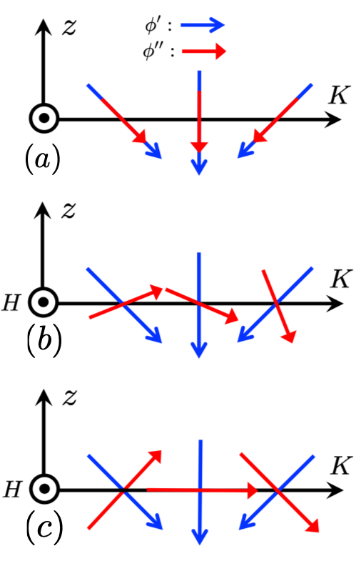
Figure 1: (color online) Helicoidal structure of the spin-triplet (spin-1) exciton field, ${\bm{\phi}}({\bm{x}})\equiv{\bm{\phi}}^{\prime}({\bm{x}})+i{\bm{\phi}}^{\prime\prime}({\bm{x}})$. The real/imaginary parts ${\bm{\phi}}^{\prime}$/${\bm{\phi}}^{\prime\prime}$ are depicted by blue/red arrow respectively. (a) helicoidal structure at the zero field (b) helicoidal structure at $h<h_{c}$, where the in-plane Zeen field is perpendicular to the paper. (c) helicoidal structure at $h>h_{c}$. The angle between the real and imaginary parts is $\pi/2$ and their amplitudes are same everywhere.

Under the in-plane Zeeman field (appendix B), the direction of the momentum $\hat{\bm{k}}$ becomes perpendicular to the Zeeman field, so that the $g$-vector can rotate around the in-plane Zeeman field (see Fig. 2(b,c)). The real and imaginary parts of the $g$-vector form a finite vector chirality along the field direction. The vector chirality is spatially uniform. The amplitude of the vector chirality becomes larger for the larger in-plane Zeeman field. Meanwhile, an angle between the real and imaginary part, $\nu$, saturates into $\pi/2$ at a critical field $h_{c}$ defined by

$$h_{c}\equiv\alpha-\frac{2}{g}+\frac{D^{2}}{4\lambda}.$$ (8)

For an in-plane Zeeman field below the critical field ($h\leq h_{c}$), the helicoid structure of the $g$-vector is given by ${\bm{\phi}}_{c}({\bm{x}})={\bm{\phi}}^{\prime}_{c}({\bm{x}})+i{\bm{\phi}}^{\prime\prime}_{c}({\bm{x}})$ with

$${\bm{\phi}}^{\prime}_{c}({\bm{x}})=\rho\cos\theta\big{(}\cos(Ky)\!\ \hat{\bm{e}}_{y}-\sin(Ky)\!\ \hat{\bm{e}}_{z}\big{)},$$ (9)

$${\bm{\phi}}^{\prime\prime}_{c}({\bm{x}})=\rho\sin\theta\big{(}\cos(Ky-\nu)\!\ \hat{\bm{e}}_{y}-\sin(Ky-\nu)\!\ \hat{\bm{e}}_{z}\big{)}.$$ (10)

Without loss of generality, we always take the field along the $x$-axis henceforth. The vector chirality formed by ${\bm{\phi}}^{\prime}_{c}$ and ${\bm{\phi}}^{\prime\prime}_{c}$ is spatially uniform, and it increases on increasing the field;

$$\sin 2\theta\sin\nu=\frac{h}{h_{c}}.$$ (11)

A ratio between $|{\bm{\phi}}^{\prime}_{c}|$ and $|{\bm{\phi}}^{\prime\prime}_{c}|$ is specified by $\theta$, and the angle between ${\bm{\phi}}^{\prime}_{c}$ and ${\bm{\phi}}^{\prime\prime}_{c}$ is specified by $\nu$. $\theta$ and $\nu$ form an energy degeneracy line under a fixed vector chirality [Eq. (11)]. When the in-plane field reaches the critical field $h_{c}$, the angle becomes $\pi/2$ and the ratio becomes the unit. Above the critical field ($h\geq h_{c}$), the angle $\nu$ takes $\pi/2$ and the ratio takes one everywhere (Fig. 2(c));

$${\bm{\phi}}_{c}({\bm{x}})=e^{iKy}\frac{\rho^{\prime}}{\sqrt{2}}(\hat{\bm{e}}_{y}+i\hat{\bm{e}}_{z}).$$ (12)

with

$$\rho^{\prime}\equiv\sqrt{\frac{h+h_{c}}{4|\gamma|}}.$$ (13)

IV low-energy collective modes

The helicoidal excitonic condensations described in the previous section break the spatial translational symmetry, spin rotational symmetry and the relative U(1) gauge symmetry; the condensate phases are accompanied by gapless Goldstone modes. Experimental observation of the collective excitations would serve as future ‘smoking-gun’ experiment for the confirmation of the excitonic condensation at the equilibrium and therefore, it is important to characterize theoretically energy-momentum dispersion of the low-energy collective modes. To this end, we take a functional derivative of the effective action (Eq. (4)) with respect to ${\bm{\phi}}$ and ${\bm{\phi}}^{\dagger}$, and derive a coupled non-linear equation of motions (EOMs) for the spin-triplet pairing field. The helicoidal structures described in the previous section are static solutions of these coupled EOMs. Thus, we consider a small fluctuation of the excitonic pairing field around these static solutions, ${\bm{\phi}}({\bm{x}})={\bm{\phi}}_{c}({\bm{x}})+\delta{\bm{\phi}}({\bm{x}})$ and ${\bm{\phi}}^{\dagger}({\bm{x}})={\bm{\phi}}^{\dagger}_{c}({\bm{x}})+\delta{\bm{\phi}}^{\dagger}({\bm{x}})$ and linearize the EOMs with respect to the fluctuation field, $\delta{\bm{\phi}}({\bm{x}})$ and $\delta{\bm{\phi}}^{\dagger}({\bm{x}})$.

As suggested by the Berry phase term in the effective action, ${\bm{\phi}}^{\dagger}\partial_{\tau}{\bm{\phi}}=i{\bm{\phi}}^{\dagger}\partial_{t}{\bm{\phi}}$, $\delta{\bm{\phi}}({\bm{x}})$ and $\delta{\bm{\phi}}^{\dagger}({\bm{x}})$ are nothing but (Holstein-Primakov) boson annihilation and creation operator respectively. Accordingly, the linearized EOMs thus obtained must reduce to a generalized eigenvalue problem with bosonic Bogoliubov de-Gennes (BdG) Hamiltonian colpa78 ;

$$|\eta|i\frac{\partial}{\partial t}\left(\begin{array}[]{c}\delta{\bm{\phi}}({\bm{x}})\\ \delta{\bm{\phi}}^{\dagger}({\bm{x}})\\ \end{array}\right)={\bm{\tau}}_{3}\hat{\bm{H}}_{\rm BdG}({\bm{\nabla}},{\bm{x}})\left(\begin{array}[]{c}\delta{\bm{\phi}}({\bm{x}})\\ \delta{\bm{\phi}}^{\dagger}({\bm{x}})\\ \end{array}\right).$$ (18)

Here ${\bm{\tau}}_{3}$ is the 2 by 2 diagonal Pauli matrix in the particle-hole space, that takes $+1$ for the annihilation and $-1$ for the creation operator. $\hat{\bm{H}}_{\rm BdG}({\bm{\nabla}},{\bm{x}})$ is a 6 by 6 matrix-formed differential operators, that are hermitian, $\hat{\bm{H}}^{\dagger}_{\rm BdG}({\bm{\nabla}},{\bm{x}})=\hat{\bm{H}}_{\rm BdG}(-{\bm{\nabla}},{\bm{x}})$. For $h\leq h_{c}$, the BdG Hamiltonian thus obtained takes the following explicit form,

$${\bm{H}}_{\rm BdG}=\left(\begin{array}[]{cccccc}-\alpha_{\nabla}&0&D\partial_{x}&-2|\gamma|\rho^{2}F_{0}&0&0\\ 0&-\alpha_{\nabla}&D\partial_{y}-ih&0&C_{y}&S_{y}\\ -D\partial_{x}&-D\partial_{y}+ih&-\alpha_{\nabla}&0&S_{y}&-C_{y}\\ -2|\gamma|\rho^{2}F^{*}_{0}&0&0&-\alpha_{\nabla}&0&D\partial_{x}\\ 0&C^{*}_{y}&S^{*}_{y}&0&-\alpha_{\nabla}&D\partial_{y}+ih\\ 0&S^{*}_{y}&-C^{*}_{y}&-D\partial_{x}&-D\partial_{y}-ih&-\alpha_{\nabla}\\ \end{array}\right).$$ (25)

For $h\geq h_{c}$, the BdG Hamiltonian is given by

$${\bm{H}}_{\rm BdG}=\left(\begin{array}[]{cccccc}-\alpha^{\prime}_{\nabla}&0&D\partial_{x}&0&0&0\\ 0&-\alpha^{\prime}_{\nabla}&D\partial_{y}+ih-i2\zeta&0&\zeta e^{2iKy}&i\zeta e^{2iKy}\\ -D\partial_{x}&-D\partial_{y}-ih+i2\zeta&-\alpha^{\prime}_{\nabla}&0&i\zeta e^{2iKy}&-\zeta e^{2iKy}\\ 0&0&0&-\alpha^{\prime}_{\nabla}&0&D\partial_{x}\\ 0&\zeta e^{-2iKy}&-i\zeta e^{-2iKy}&0&-\alpha^{\prime}_{\nabla}&D\partial_{y}-ih+i2\zeta\\ 0&-i\zeta e^{-2iKy}&-\zeta e^{-2iKy}&-D\partial_{x}&-D\partial_{y}+ih-i2\zeta&-\alpha^{\prime}_{\nabla}\\ \end{array}\right),$$ (32)

with

$$\zeta \equiv 2|\gamma|{\rho^{\prime}}^{2},$$ (33)

$$\alpha_{\nabla} \equiv\alpha-\frac{2}{g}-4|\gamma|\rho^{2}+\lambda{\nabla}^{2},$$ (34)

$$\alpha^{\prime}_{\nabla} \equiv\alpha-\frac{2}{g}-4|\gamma|{\rho^{\prime}}^{2}+\lambda{\nabla}^{2},$$ (35)

$$F_{0} =\cos 2\theta+i\sin 2\theta\cos\nu,$$ (36)

$$C_{y} \equiv\frac{h_{c}}{2}\big{(}e^{i2Ky}F_{+}+e^{-i2Ky}F_{-}\big{)},$$ (37)

$$S_{y} \equiv i\frac{h_{c}}{2}\big{(}e^{i2Ky}F_{+}-e^{-i2Ky}F_{-}\big{)},$$ (38)

$$F_{\pm} \equiv\cos^{2}\theta-\sin^{2}\theta e^{\mp i2\nu}+i\sin 2\theta e^{\mp i\nu}.$$ (39)

$K$, $\rho$, $\rho^{\prime}$ and $h_{c}$ are already defined by Eqs. (7,13,8) respectively. $\theta$ and $\nu$ in Eqs. (36,39) must satisfy Eq. (11). Note that the two BdG Hamiltonians beome identical to each other at $h=h_{c}$, where $F_{0}=0$, $F_{+}=2$, $F_{-}=0$. Using bosonic Bogoliubov transformations colpa78 , we diagonalize these Hamiltonians in the momentum space, to obtain energy-momentum dispersions of the low-energy collective excitations in the helicoidal excitonic phases (Appendix C). Fig. 2 shows the dispersions along the high symmetric line in the momentum space for $h=0$, $h<h_{c}$ and $h>h_{c}$ respectively.

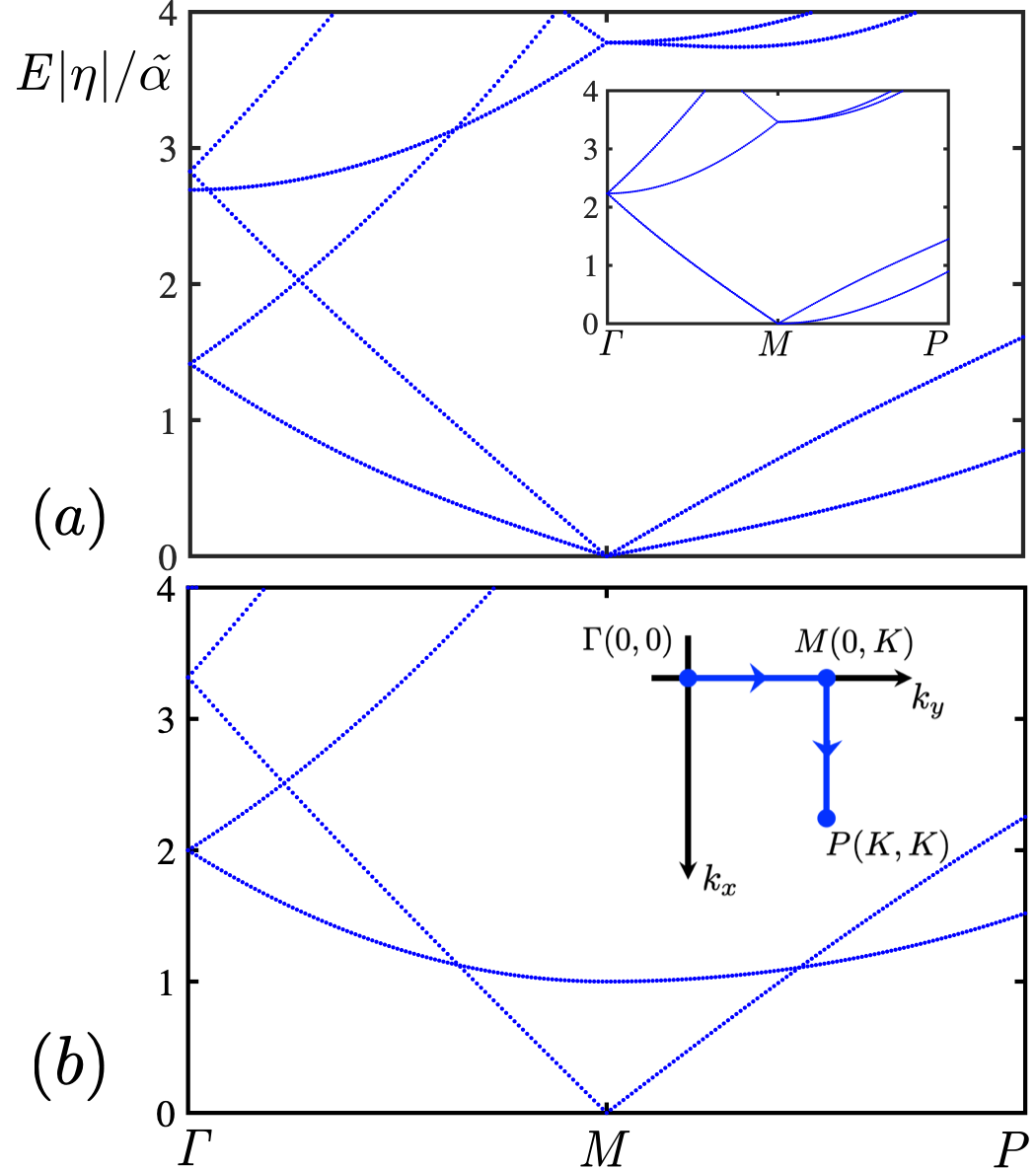
Figure 2: (color online) Energy-momentum dispersions of the low-energy collective modes in the helicoidal excitonic condensate phases. The dispersions are plotted along the high symmetric line (shown in the inset of (b)). The unit of the energy axis is $\tilde{\alpha}/|\eta|$ where $\tilde{\alpha}\equiv\alpha-\frac{2}{g}$. (a) The dispersion for $h<h_{c}$ where $\tilde{\alpha}=1,|\eta|=1,\lambda=1,D=2,h=1.5$ (inset is for $h=0$). (b) The dispersion for $h>h_{c}$, where $\tilde{\alpha}=1,|\eta|=1,\lambda=1,D=2,h=3$.

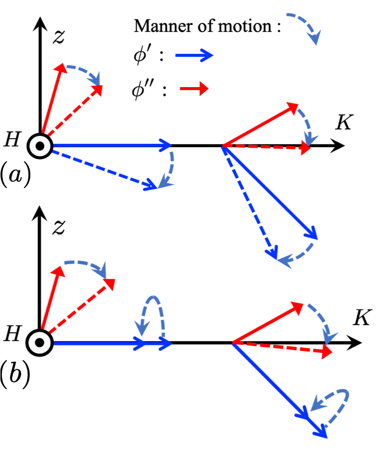
Figure 3: (color online) Schematic pictures of (a) translational mode and (b) spin rotational mode

The helicoidal condensate phase at $h\leq h_{c}$ has two gapless Goldstone modes around ${\bm{k}}=(0,K)$; translational mode and spin rotational mode (Fig. 2(a)). These two result from the spontaneous symmetry breakings of the continuous symmetries; translational symmetry and a combined symmetry of the relative gauge symmetry and the spin rotation symmetry respectively. The translational mode at the gapless point induces a simultaneous rotation of ${\bm{\phi}}^{\prime}$ and ${\bm{\phi}}^{\prime\prime}$ by the same angle around the $yz$ plane (Fig. 3(a)). The spin rotational mode induces a change of the amplitudes of ${\bm{\phi}}^{\prime}$ and ${\bm{\phi}}^{\prime\prime}$ as well as the relative angle between these two vectors (Fig. 3(b)), but it does not change the total amplitude of the spin-1 exciton field, $|{\bm{\phi}}|^{2}\equiv|{\bm{\phi}}^{\prime}|^{2}+|{\bm{\phi}}^{\prime\prime}|^{2}$. When the field is above the critical field ($h\geq h_{c}$), the relative angle between the real and imaginary part is locked to $\pi/2$ by the large in-plane field; the angle between these two are fully saturated (‘fully saturated phase’). Accordingly, the spin rotational mode acquires a finite mass and only the translational mode forms a gapless dispersion at ${\bm{k}}=(0,K)$ (See Fig. 2(b)).

Finally, let us give several remarks on light scatterings for probing these low-energy collective modes in the EHDL system. In the layered heterostructure, the electron and hole layers are physically well separated by an intermediate separation layer with its thickness being typically 10 nm wu19 . Meanwhile, single exciton is a pair of the electron creation and the hole creation. Thus, generally, the external electromagnetic field can couple with the exciton in the EHDL system only through 2-excitons process, 4-excitons process, and so on; one photon causes at least a pair of exciton creation and exciton annihilation in the EHDL system. A calculation in appendix D shows that the (static) helicoidal excitonic order parameter quadratically induces a uniform change of the electron density in the electron layer, $\delta\rho^{e}(\bm{x})\equiv\delta\langle a^{\dagger}_{\alpha}({\bm{x}})a_{\alpha}({\bm{x}})\rangle\sim\rho^{2}$. This suggests that photon can couple electrically with the low-energy collective modes in the helicoidal excitonic condensate in EHDL system.

V experimental probes

In the presence of a small Dirac term in the hole layer $(\Delta_{h}\neq 0)$, the helicoidal texture of the spin-1 exciton condensate induces a helicoidal texture of local magnetic moment in the electron layer, whose spatial pitch is $1/2K$ instead of $1/K$. At the zero magnetic field, however, the helicoid structure given by Eq. (5) is symmetric under the time-reversal symmetry combined with a gauge transformation for the electron or hole band. Thus, the local magnetic moment in each layer is quenched at $H=0$.

The helicoidal magnetic texture appears when the in-plane Zeeman field $H$ is applied to the helicoidal excitonic phase. Thereby, the local magnetic moment as well as the spin-1 exciton field rotate around the in-plane Zeeman field;

$${\bm{m}}^{e}({\bm{x}})\equiv\langle a^{\dagger}_{\alpha}({\bm{x}})[{\bm{\sigma}}]_{\alpha\beta}a_{\beta}({\bm{x}})\rangle$$

$$=A(H)\big{(}\cos^{2}\theta\cos(2Ky)+\sin^{2}\theta\cos(2Ky-2\nu)\big{)}\hat{\bm{e}}_{y}-$$

$$B(H)\big{(}\cos^{2}\theta\sin(2Ky)+\sin^{2}\theta\sin(2Ky-2\nu)\big{)}\hat{\bm{e}}_{z}+\cdots.$$ (40)

Here $A(H)$ and $B(H)$ are real-valued and odd functions in the magnetic field $H$; $A(-H)=-A(H)$, $B(-H)=-B(H)$. ‘$\cdots$’ in the right-hand side denotes the higher order harmonic contributions ($4Ky$, $6Ky$, $\cdots$ components). In the leading order in small $\Delta_{h}$, $A$ and $B$ are proportional to $\rho^{2}\Delta_{h}$ (Appendix D).

Having a finite out-of-plane (${\bm{e}}_{z}$-component) magnetization, the spatial magnetic texture given in Eq. (40) could be experimentally seen by magnetic optical measurements hubert98 . For example, when the electron layer is sufficiently reflective, a spatial map of the magnetic Kerr rotational angle in the two-dimensional layer must show a stripe structure. According to our theory prediction, the magnetic stripe appears in parallel to the in-plane Zeeman field, and it disappears when the field is set zero. The Kerr rotation angle changes its sign when the in-plane field is reversed.

VI conclusion and discussion

A recent transport experiment on a strained layered InAs/AlSb/GaInSb heterostructure reports resistive signatures of the excitonic coupling at low temperature around the charge neutrality line of the BEC regime wu19 . In this paper, we show that due to the large Rashba interaction in the electron layer, energy degeneracy among three spin-1 (spin-triplet) exciton bands are lifted at finite momentum. On lowering the temperature or on changing the charge state energy, the lowest spin-1 exciton band can undergo the BEC at finite momentum, resulting in a helicoidal structure of the spin-1 exciton field (helicoidal excitonic condensate). The helicoidal plane of the spin-1 exciton can be controlled by the in-plane Zeeman field.

Based on the linearized coupled EOMs of the spin-1 exciton, we calculate momentum-energy dispersions of the low-energy collective modes in the helicoidal excitonic phase. For future possible light scattering experiments, we show that these low-energy modes can couple electrically with one photon through the two-excitons processes. We also demonstrate that due to small Dirac term in the heavy hole layer, the helicoidal structure of the spin-1 exciton condensate results in a helicoidal magnetic structure in the electron layer. Having a finite out-of-plane magnetization, the helicoidal magnetic structure could be visualized by a spatial map of the magnetic Kerr rotation angle in the two-dimensional layer. Our theory predicts that the magnetic stripes appear in parallel to the in-plane Zeeman field and it disappears at the zero Zeeman field.

In a Coulomb coupled EHDL system without the SOI, the spin triplet (spin-1) excitons and spin singlet (spin-0) exciton are energetically degenerate due to the independent spin rotations of electron spin and hole spin zhu96 . Meanwhile, the analyses in this paper has ignored a coupling between the spin-0 exciton and spin-1 excitons. The coupling does exist at the first order in the Rashba term in the electron layer $\xi_{e}$ as well as at the first order in the in-plane Zeeman field $H$;

$$S =\cdots-D\int d{\bm{x}}\!\ \Big{[}\hat{\bm{e}}_{y}\cdot\big{(}{\bm{\phi}}^{\dagger}\times\partial_{x}{\bm{\phi}}\big{)}-\hat{\bm{e}}_{x}\cdot\big{(}{\bm{\phi}}^{\dagger}\times\partial_{y}{\bm{\phi}}\big{)}\Big{]}$$

$$+D\int d{\bm{x}}\!\ \Big{[}\phi^{\dagger}_{x}i\partial_{y}\phi_{0}+\phi^{\dagger}_{0}i\partial_{y}\phi_{x}-\phi^{\dagger}_{y}i\partial_{x}\phi_{0}-\phi^{\dagger}_{0}i\partial_{x}\phi_{y}\Big{]}$$

$$+ih\int d{\bm{x}}\!\ \hat{\bm{e}}_{H}\cdot\big{(}{\bm{\phi}}^{\dagger}\times{\bm{\phi}}\big{)}+h^{\prime}\int d{\bm{x}}\!\ \hat{\bm{e}}_{H}\cdot\big{(}{\bm{\phi}}^{\dagger}\phi_{0}+\phi^{\dagger}_{0}{\bm{\phi}}\big{)},$$ (41)

Here ${\bm{\phi}}$ and $\phi_{0}$ denote the spin-1 and spin-0 exciton fields respectively. The first and third terms are nothing but the last three terms in Eq. (4). $h$ and $h^{\prime}$ are proportional to the in-plane field $H$, $h\neq h^{\prime}$. At the quadratic level of the effective action at the zero field ($h=h^{\prime}=0$), the four-fold degenerate exciton bands at the zero momentum (one spin-0 and three spin-1) are split into two doubly degenerate exciton bands at finite momentum ${\bm{k}}$;

$$H_{{\rm EX}}=\sum_{\bm{k}}\left(\begin{array}[]{cccc}\phi^{\dagger}_{0}({\bm{k}})&\phi^{\dagger}_{x}({\bm{k}})&\phi^{\dagger}_{y}({\bm{k}})&\phi^{\dagger}_{z}({\bm{k}})\\ \end{array}\right)\left(\begin{array}[]{cccc}\beta_{\bm{k}}&-k_{y}D&k_{x}D&0\\ -k_{y}D&\beta_{\bm{k}}&0&ik_{x}D\\ k_{x}D&0&\beta_{\bm{k}}&ik_{y}D\\ 0&-ik_{x}D&-ik_{y}D&\beta_{\bm{k}}\\ \end{array}\right)\left(\begin{array}[]{c}\phi_{0}({\bm{k}})\\ \phi_{x}({\bm{k}})\\ \phi_{y}({\bm{k}})\\ \phi_{z}({\bm{k}})\\ \end{array}\right),$$ (51)

with $\beta_{\bm{k}}\equiv-\alpha+2/g+\lambda k^{2}>0$. The upper two exciton bands have an energy of $\beta_{\bm{k}}+D|{\bm{k}}|$, and the lower two exciton bands have an energy of $\beta_{\bm{k}}-D|{\bm{k}}|$. One of the lower two bands is a mixture of purely three spin-1 excitons, $\phi_{z}+i(\hat{k}_{x}\phi_{x}+\hat{k}_{y}\phi_{y})$, whose BEC induces the helicoidal excitonic phase [discussed in this paper]. On the one hand, the other of the lower two bands is a mixture of the spin-0 and spin-1 exciton bands, $\phi_{0}-(-\hat{k}_{y}\phi_{x}+\hat{k}_{x}\phi_{y})$, whose BEC induces an in-plane collinear texture of the spin-1 exciton field. The collinear texture and the helicoidal texture are energetically degenerate at the zero Zeeman field in the absence of the Dirac term in hole layer ($\Delta_{h}=H=0$). The energy degeneracy is due to the $\pi$ spin-rotation around the $z$-axis only in the hole band; ${\bm{b}}^{\dagger}_{\bm{k}}\rightarrow{\bm{b}}^{\dagger}_{\bm{k}}{\bm{\sigma}}_{z}$ in Eqs. (1,2). The degeneracy is lifted by the Dirac term in the hole band $\Delta_{h}$ as well as the in-plane Zeeman field. In the presence of these perturbations, a mixture of these two textures will be selected as a true classical ground state. By construction, the mixture has lower symmetries than the helicoidal excitonic phase discussed in this paper and thereby it has essentially the same physical response as the helicoidal phase [Sec. VI and Sec. V]. Nonetheless, detailed physical properties of the mixed phase need more theoretical studied and will be discussed elsewhere.

Appendix A derivation of the effective action

In this appendix, we derive an effective $\phi^{4}$ action for the spin-triplet (spin-1) exciton field in the presence of the SOI and the Zeeman field. We begin with the partition function $Z$ for Eq. (1,2,3) with $\Delta_{h}=0$,

$$Z=\int\prod{\cal D}{\bm{a}}^{\dagger}_{k}{\cal D}{\bm{a}}_{k}{\cal D}{\bm{b}}^{\dagger}_{k}{\cal D}{\bm{b}}_{k}\exp\big{[}-S[{\bm{a}},{\bm{b}}]\big{]}$$

where the effective action $S$ is given by

$$S[{\bm{a}},{\bm{b}}]=\sum_{k}\left(\begin{array}[]{cc}{\bm{a}}^{\dagger}_{k}&{\bm{b}}^{\dagger}_{k}\\ \end{array}\right)\!\ \big{(}G^{-1}_{0}(k)+G^{-1}_{\rm R}(k)+G^{-1}_{H}(k)\big{)}\!\ \left(\begin{array}[]{c}{\bm{a}}_{k}\\ {\bm{b}}_{k}\\ \end{array}\right)-\frac{g}{2}\sum_{k}\sum_{m=0,x,y,z}{\cal O}^{\dagger}_{m}(k){\cal O}_{m}(k)\Big{]}.$$ (55)

Here non-interacting temperature Green function, Rashba and Zeeman field parts take forms of,

$$G^{-1}_{0}(k) \equiv\left(\begin{array}[]{cc}(-i\omega_{n}+{\cal E}_{a}({\bm{k}})-\mu){\bm{\sigma}}_{0}&\\ &(-i\omega_{n}+{\cal E}_{b}({\bm{k}})-\mu){\bm{\sigma}}_{0}\\ \end{array}\right),$$ (58)

$$G^{-1}_{\rm R}(k) \equiv\left(\begin{array}[]{cc}\xi_{e}(k_{y}{\bm{\sigma}}_{x}-k_{x}{\bm{\sigma}}_{y})&\\ &0\\ \end{array}\right),\ \ G^{-1}_{H}(k)\equiv\left(\begin{array}[]{cc}H{\bm{\sigma}}_{H}&\\ &H{\bm{\sigma}}_{H}\\ \end{array}\right),$$ (63)

with ${\cal E}_{a}({\bm{k}})\equiv\hbar^{2}{\bm{k}}^{2}/2m_{e}-E_{g}$, ${\cal E}_{b}({\bm{k}})\equiv-\hbar^{2}{\bm{k}}^{2}/2m_{h}+E_{g}$, and $k\equiv(i\omega_{n},{\bm{k}})$. Note that we used the following Fourier transformation for ${\bm{a}}({\bm{x}},\tau)$, ${\bm{b}}({\bm{x}},\tau)$ and ${\cal O}({\bm{x}},\tau)$,

$$f({\bm{x}},\tau)=\frac{1}{\sqrt{\beta V}}\sum_{k}e^{i{\bm{k}}{\bm{x}}-i\omega_{n}\tau}f(k).$$ (64)

$\beta$ is an inverse temperature, $\beta\equiv 1/(k_{\rm B}T)$, $i\omega_{n}=(2n+1)\pi/\beta$ for ${\bm{a}}$ and ${\bm{b}}$, $i\omega_{n}=2n\pi/\beta$ for ${\cal O}$, and $\sum_{k}\equiv\sum_{\bm{k}}\sum_{\omega_{n}}$.

A decomposition of the interaction by the Stratonovich Hubbard (SH) variables ${\bm{\phi}}(k)$ fradkin91 gives out a quadratic form of the ${\bm{a}}$ and ${\bm{b}}$ fields,

$$\exp\Big{[}\frac{g}{2}\sum_{k}\sum^{z}_{m=0}{\cal O}^{\dagger}_{m}(k){\cal O}_{m}(k)\Big{]}$$

$$\hskip 14.22636pt=\int{\cal D}{\bm{\phi}}^{\dagger}{\cal D}{\bm{\phi}}\!\ \exp\Big{[}-\sum_{k}\frac{2}{g}|{\bm{\phi}}_{k}|^{2}$$

$$\hskip 28.45274pt+\sum_{k}\big{(}{\bm{\phi}}^{\dagger}(k)\cdot{\cal O}(k)+{\cal O}^{\dagger}(k)\cdot{\bm{\phi}}(k)\big{)}\Big{]}.$$ (65)

A gaussian integration over the ${\bm{a}}$ and ${\bm{b}}$ fields leads to a functional of the SH variables. A Taylor expansion of the functional with respect to the SH variables gives,

$$Z=\int{\cal D}{\bm{\phi}}^{\dagger}{\cal D}{\bm{\phi}}\!\ \exp\Big{[}-\sum_{k}\frac{2}{g}|{\bm{\phi}}_{k}|^{2}$$

$$\hskip 22.76228pt+{\rm Tr}\big{[}{\bm{1}}+G_{0}(k)\!\ G^{-1}_{\rm R}(k)\!\ \delta_{k,k^{\prime}}$$

$$\hskip 34.14322pt+G_{0}(k)\!\ G^{-1}_{H}(k)\!\ \delta_{k,k^{\prime}}-G_{0}(k)\!\ {\Phi}_{q}\!\ \delta_{k,k+q}\big{]}\Big{]}$$

$$=\int{\cal D}{\bm{\phi}}^{\dagger}{\cal D}{\bm{\phi}}\!\ \exp\Big{[}-\sum_{k}\frac{2}{g}|{\bm{\phi}}_{k}|^{2}$$

$$\hskip 22.76228pt+{\rm Tr}\big{[}G_{0}G^{-1}_{\rm R}G_{0}{\Phi}G_{0}{\Phi}+G_{0}G^{-1}_{H}G_{0}{\Phi}G_{0}{\Phi}$$

$$\hskip 34.14322pt-\frac{1}{2}G_{0}{\Phi}G_{0}{\Phi}-\frac{1}{4}G_{0}{\Phi}G_{0}{\Phi}G_{0}{\Phi}G_{0}{\Phi}\big{]}\Big{]},$$ (66)

where

$${\Phi}_{q}=\frac{1}{\sqrt{\beta V}}\left(\begin{array}[]{cc}0&\sum_{m}\phi_{m}(-q){\bm{\sigma}}_{m}\\ \sum_{m}\phi^{\dagger}_{m}(q){\bm{\sigma}}_{m}&0\\ \end{array}\right).$$ (69)

In the expansion, we took into account only the first order in the small $\xi_{e}$ and $H$. We also expand Eq. (66) in small $q\equiv(i\epsilon_{n},{\bm{q}})$, to keep up to ${\cal O}({\bm{q}}^{2},i\epsilon_{n})$ in ${\rm Tr}[G_{0}{\Phi}G_{0}{\Phi}]$, up to ${\cal O}({\bm{q}}^{1},i\epsilon_{n}^{0})$ in ${\rm Tr}[G_{0}G^{-1}_{\rm R}G_{0}{\Phi}G_{0}{\Phi}]$, and up to ${\cal O}({\bm{q}}^{0},i\epsilon_{n}^{0})$ in the other terms. This gives Eq. (4) as the effective action for the spin-1 exciton field. The coefficients in Eq. (4) are calculated in the followings,

$$-\alpha +\lambda{\bm{q}}^{2}+\cdots=\frac{2}{V}\sum_{\bm{k}}\frac{n_{\rm F}({\cal E}_{a}({\bm{k}}))-n_{\rm F}({\cal E}_{b}({\bm{k}}+{\bm{q}}))}{{\cal E}_{a}({\bm{k}})-{\cal E}_{b}({\bm{k}}+{\bm{q}})},$$

$$\eta =-\frac{2}{V}\sum_{\bm{k}}\bigg{\{}\frac{n_{\rm F}({\cal E}_{b}({\bm{k}}))-n_{\rm F}({\cal E}_{a}({\bm{k}}))}{({\cal E}_{a}({\bm{k}})-{\cal E}_{b}({\bm{k}}))^{2}}$$

$$-\frac{\beta}{2+2\cosh(\beta({\cal E}_{a}({\bm{k}})-\mu))}\frac{1}{{\cal E}_{a}({\bm{k}})-{\cal E}_{b}({\bm{k}})}\bigg{\}}<0,$$

$$\gamma =-\frac{1}{V}\sum_{\bm{k}}\bigg{(}\frac{1}{{\cal E}_{a}-{\cal E}_{b}}\bigg{)}^{2}\bigg{\{}2\frac{n_{\rm F}({\cal E}_{b})-n_{\rm F}({\cal E}_{a})}{{\cal E}_{a}-{\cal E}_{b}}$$

$$-\frac{\beta}{2+2\cosh(\beta({\cal E}_{b}-\mu))}-\frac{\beta}{2+2\cosh(\beta({\cal E}_{a}-\mu))}\bigg{\}}<0,$$

$$D =-\frac{\xi_{e}}{V}\sum_{\bm{k}}\frac{\hbar^{2}k^{2}_{x}}{m_{h}}\bigg{(}\frac{1}{{\cal E}_{a}-{\cal E}_{b}}\bigg{)}^{2}\bigg{\{}4\frac{n_{\rm F}({\cal E}_{b})-n_{\rm F}({\cal E}_{a})}{{\cal E}_{a}-{\cal E}_{b}}$$

$$-\frac{\beta}{1+\cosh(\beta({\cal E}_{b}-\mu))}-\frac{\beta}{1+\cosh(\beta({\cal E}_{a}-\mu))}\bigg{\}},$$

$$h =\frac{2H}{V}\sum_{\bm{k}}\frac{1}{{\cal E}_{a}-{\cal E}_{b}}\bigg{\{}2\frac{n_{\rm F}({\cal E}_{a})-n_{\rm F}({\cal E}_{b})}{{\cal E}_{a}-{\cal E}_{b}}$$

$$+\frac{\beta}{2+2\cosh(\beta({\cal E}_{b}-\mu))}+\frac{\beta}{2+2\cosh(\beta({\cal E}_{a}-\mu))}\bigg{\}}.$$

From these expressions, we can see that both $\alpha$ and $\lambda$ are positive. Since $D$ and $h$ are proportional to $\xi_{e}$ and $H$ respectively, we can assume that $D$ and $h$ are positive without loss of generality.

Appendix B minimization of the classical action

In this appendix, we minimize the classical energy in Eq. (4) with respect to the real and imaginary parts of the spin-1 exciton field, ${\bm{\phi}}={\bm{\phi}}^{\prime}+i{\bm{\phi}}^{\prime\prime}$. Take ${\bm{\phi}}^{\prime}=A{\bm{n}}^{\prime}$ and ${\bm{\phi}}^{\prime\prime}=B{\bm{n}}^{\prime\prime}$ with unit vectors ${\bm{n}}^{\prime}$ and ${\bm{n}}^{\prime\prime}$ ; $|{\bm{n}}^{\prime}|=|{\bm{n}}^{\prime\prime}|=1$. In the absence of the SOI, the exciton field takes a spatially uniform solution, because $\lambda>0$. Thereby, the real and imaginary parts are parallel to each other in the spin space;

$${\bm{\phi}}^{\prime}_{c}+i{\bm{\phi}}^{\prime\prime}_{c}=\frac{1}{2|\gamma|}\Big{(}\alpha-\frac{2}{g}\Big{)}e^{i\theta}{\bm{n}},$$ (70)

The solution breaks the two global symmetries. The U(1) symmetry associated with $\theta$ is nothing but a difference between the U(1) gauge degree of freedom of the electron and that of the hole. The SO(3) symmetry associate with ${\bm{n}}$ represents the global spin rotational symmetry. In the following, we study how the uniform solution would be deformed in the presence of finite SOI ($D\neq 0$).

B.1 $H=0$ and $D\neq 0$

In the presence of the SOI, the spin-1 exciton field takes a spatially dependent solution. Spatial gradients of the amplitudes, $A$ and $B$, do not lower the SOI energy. Accordingly, without loss of generality, we can assume that the amplitudes are spatially uniform and the unit vectors depend on the space coordinate ${\bm{x}}$;

$${\bm{\phi}}^{\prime} =A{\bm{n}}^{\prime}({\bm{x}}),$$ (71)

$${\bm{\phi}}^{\prime\prime} =B{\bm{n}}^{\prime\prime}({\bm{x}}).$$ (72)

This gives the following functional for the classical action, where $V$ and $\beta$ are the volume of the system and the inverse temperature respectively;

$$\frac{1}{\beta V}S[A,B,{\bm{n}}^{\prime}({\bm{x}}),{\bm{n}}^{\prime\prime}({\bm{x}})]$$

$$\ \ \ =-\big{(}\alpha-\frac{2}{g}\big{)}\big{(}A^{2}+B^{2}\big{)}-\gamma\big{(}A^{4}+B^{4}+6A^{2}B^{2}\big{)}$$

$$\ \ -\frac{A^{2}}{V}C_{1}[{\bm{n}}^{\prime}]-\frac{B^{2}}{V}C_{1}[{\bm{n}}^{\prime\prime}]+4\gamma\frac{A^{2}B^{2}}{V}C_{2}[{\bm{n}}^{\prime},{\bm{n}}^{\prime\prime}].$$ (73)

Here $C_{1}$ are $C_{2}$ are functionals of the unit vectors,

$$C_{1}[{\bm{n}}^{\prime}]\equiv \int d{\bm{x}}\Big{[}-\lambda|{\nabla}{\bm{n}}^{\prime}|^{2}$$

$$+D\big{(}{\bm{e}}_{y}\cdot({\bm{n}}^{\prime}\times\partial_{x}{\bm{n}}^{\prime})-{\bm{e}}_{x}\cdot({\bm{n}}^{\prime}\times\partial_{y}{\bm{n}}^{\prime})\big{)}\Big{]},$$ (74)

$$C_{2}[{\bm{n}}^{\prime},{\bm{n}}^{\prime\prime}] \equiv\int d{\bm{x}}\!\ \big{(}{\bm{n}}^{\prime}\cdot{\bm{n}}^{\prime\prime}\big{)}^{2}.$$ (75)

For the later convenience, let us rotate ${\bm{n}}^{\prime}$ and ${\bm{n}}^{\prime\prime}$ by $\pi/2$ around the $z$-axis;

$${\bm{n}}^{\prime(\prime\prime)}_{\rm new}({\bm{x}})=\left(\begin{array}[]{ccc}0&-1&0\\ 1&0&0\\ 0&0&1\\ \end{array}\right){\bm{n}}^{\prime(\prime\prime)}_{\rm old}({\bm{x}}).$$ (79)

In the rotated frame, $C_{1}$ and $C_{2}$ are given by

$$C_{1}[{\bm{n}}^{\prime}]= \int d{\bm{x}}\Big{[}-\lambda|{\bm{\nabla}}{\bm{n}}^{\prime}|^{2}+D{\bm{n}}^{\prime}\cdot({\bm{\nabla}}\times{\bm{n}}^{\prime})\Big{]}$$ (80)

$$C_{2}[{\bm{n}}^{\prime},{\bm{n}}^{\prime\prime}] =\int d{\bm{x}}\!\ \big{(}{\bm{n}}^{\prime}\cdot{\bm{n}}^{\prime\prime}\big{)}^{2}.$$ (81)

with ${\bm{\nabla}}\equiv(\partial_{x},\partial_{y},0)$.

In the following, we first minimize the classical action for fixed $A$ and $B$ (Eq. (73)). To this end, we have only to maximize $C_{1}[{\bm{n}}^{\prime}]$, $C_{1}[{\bm{n}}^{\prime\prime}]$ and $C_{2}[{\bm{n}}^{\prime},{\bm{n}}^{\prime\prime}]$ with respect to ${\bm{n}}^{\prime}$ and ${\bm{n}}^{\prime\prime}$, because $\gamma<0$. These three functionals can be simultaneously maximized.

To see this, let us first maximize $C_{1}[{\bm{n}}]$ under the normalization condition of $|{\bm{n}}({\bm{x}})|=1$ for any ${\bm{x}}$. In the momentum-space representation, the Fourier series of ${\bm{n}}({\bm{x}})$ comprises of two real-valued vectors, ${\bm{\alpha}}_{\bm{k}}$ and ${\bm{\beta}}_{\bm{k}}$,

$${\bm{n}}({\bm{x}}) =\sum_{\bm{k}}e^{i{\bm{k}}{\bm{x}}}\frac{1}{2}\big{(}{\bm{\alpha}}_{\bm{k}}+i{\bm{\beta}}_{\bm{k}}\big{)}$$

$$=\sum_{k_{x}>0}\big{(}\cos({\bm{k}}{\bm{x}}){\bm{\alpha}}_{\bm{k}}-\sin({\bm{k}}{\bm{x}}){\bm{\beta}}_{\bm{k}}\big{)},$$ (82)

with ${\bm{\alpha}}_{\bm{k}}={\bm{\alpha}}_{-{\bm{k}}}$ and ${\bm{\beta}}_{\bm{k}}=-{\bm{\beta}}_{-{\bm{k}}}$. In terms of these vectors, $C_{1}[{\bm{n}}]$ takes a form of

$$C_{1}[{\bm{n}}]=V\sum_{k_{x}>0}\Big{[}-\frac{\lambda}{2}\big{(}|{\bm{\alpha}}_{\bm{k}}|^{2}+|{\bm{\beta}}_{\bm{k}}|^{2}\big{)}k^{2}+D{\bm{k}}\cdot\big{(}{\bm{\alpha}}_{\bm{k}}\times{\bm{\beta}}_{\bm{k}}\big{)}\Big{]}.$$ (83)

The normalization condition imposes a global constraint onto the Fourier series;

$$\frac{1}{V}\int d{\bm{x}}\!\ |{\bm{n}}({\bm{x}})|^{2} =\frac{1}{2}\sum_{k_{x}>0}\big{(}|{\bm{\alpha}}_{\bm{k}}|^{2}+|{\bm{\beta}}_{\bm{k}}|^{2}\big{)}$$

$$\equiv\frac{1}{2}\sum_{k_{x}>0}w^{2}_{\bm{k}}=1.$$ (84)

Under Eq. (84), Eq. (83) is maximized by

$${\bm{n}}({\bm{x}})=\sum^{k_{x}>0}_{|{\bm{k}}|=D/2\lambda}\frac{w_{\bm{k}}}{\sqrt{2}}\big{(}\cos({\bm{k}}{\bm{x}})\hat{\bm{k}}_{\perp,1}-\sin({\bm{k}}{\bm{x}})\hat{\bm{k}}_{\perp,2}\big{)},$$ (85)

where $|{\bm{\alpha}}_{\bm{k}}|^{2}+|{\bm{\beta}}_{\bm{k}}|^{2}\equiv w^{2}_{\bm{k}}$ and ${\bm{k}}=k\hat{\bm{k}}$. The three unit vectors $\hat{\bm{k}},\hat{\bm{k}}_{\perp,1}$ and $\hat{\bm{k}}_{\perp,2}$ form the right-handed coordinate system, $\hat{\bm{k}}_{\perp,1}\times\hat{\bm{k}}_{\perp,2}=\hat{\bm{k}}$.

To satisfy $|{\bm{n}}({\bm{x}})|=1$ for every ${\bm{x}}$, the right-hand side of Eq. (85) must have only one momentum component. Suppose that it has two momentum components, ${\bm{k}}$ and ${\bm{k}}^{\prime}$,

$${\bm{n}}({\bm{x}}) =\frac{w}{\sqrt{2}}\big{(}\cos({\bm{k}}{\bm{x}})\hat{\bm{k}}_{\perp,1}-\sin({\bm{k}}{\bm{x}})\hat{\bm{k}}_{\perp,2}\big{)}$$

$$\ \ +\frac{w^{\prime}}{\sqrt{2}}\big{(}\cos({\bm{k}}^{\prime}{\bm{x}})\hat{\bm{k}}^{\prime}_{\perp,1}-\sin({\bm{k}}^{\prime}{\bm{x}})\hat{\bm{k}}^{\prime}_{\perp,2}\big{)}.$$ (86)

Without loss of generality, we can take from Eq. (85) as follows,

$$\left\{\begin{array}[]{c}{\bm{k}}=\frac{D}{2\lambda}{\bm{e}}_{x}\\ \hat{\bm{k}}_{\perp,1}={\bm{e}}_{y}\\ \hat{\bm{k}}_{\perp,2}={\bm{e}}_{z}\\ \end{array}\right.,\ \left\{\begin{array}[]{l}{\bm{k}}^{\prime}=\frac{D}{2\lambda}\big{(}c_{\gamma}{\bm{e}}_{x}+s_{\gamma}{\bm{e}}_{y}\big{)}\\ \hat{\bm{k}}^{\prime}_{\perp,1}=c_{\nu}(-s_{\gamma}{\bm{e}}_{x}+c_{\gamma}{\bm{e}}_{y})+s_{\nu}{\bm{e}}_{z}\\ \hat{\bm{k}}^{\prime}_{\perp,2}=s_{\nu}(s_{\gamma}{\bm{e}}_{x}-c_{\gamma}{\bm{e}}_{y})+c_{\nu}{\bm{e}}_{z}\\ \end{array}\right..$$ (93)

Here $c_{\nu}\equiv\cos\nu$, $s_{\nu}\equiv\sin\nu$, $c_{\gamma}\equiv\cos\gamma$, and $s_{\gamma}\equiv\sin\gamma$. Then, we have

$$|{\bm{n}}({\bm{x}})|^{2}=\frac{1}{2}\big{(}w^{2}+{w^{\prime}}^{2}\big{)}+ww^{\prime}\Big{\{}$$

$$c_{\nu}(c_{\gamma}-1)\cos\big{(}({\bm{k}}+{\bm{k}}^{\prime}){\bm{x}}\big{)}+c_{\nu}(c_{\gamma}+1)\cos\big{(}({\bm{k}}-{\bm{k}}^{\prime}){\bm{x}}\big{)}+$$

$$s_{\nu}(c_{\gamma}-1)\sin\big{(}({\bm{k}}+{\bm{k}}^{\prime}){\bm{x}}\big{)}-s_{\nu}(c_{\gamma}+1)\sin\big{(}({\bm{k}}-{\bm{k}}^{\prime}){\bm{x}}\big{)}\Big{\}}.$$

To make the right-hand side to be independent of ${\bm{x}}$, we must have

$$c_{\nu}(c_{\gamma}-1)=c_{\nu}(c_{\gamma}+1)=s_{\nu}(c_{\gamma}-1)=s_{\nu}(c_{\gamma}+1)=0.$$ (94)

Nonetheless, Eq. (94) cannot be achieved by any $\gamma\in[0,2\pi)$ and $\nu\in[0,2\pi)$; this requires $ww^{\prime}=0$; the right hand side of Eq. (85) must have only one momentum component ${\bm{k}}$ with $w_{\bm{k}}=\sqrt{2}$.

$C_{1}[{\bm{n}}^{\prime}]$, $C_{1}[{\bm{n}}^{\prime\prime}]$ and $C_{2}[{\bm{n}}^{\prime},{\bm{n}}^{\prime\prime}]$ are simultaneously maximized by

$${\bm{n}}^{\prime}({\bm{x}})={\bm{n}}^{\prime\prime}({\bm{x}})=\cos({\bm{k}}{\bm{x}})\hat{\bm{k}}_{\perp,1}-\sin({\bm{k}}{\bm{x}})\hat{\bm{k}}_{\perp,2}.$$ (95)

with ${\bm{k}}=D/(2\lambda)\hat{\bm{k}}$ and $\hat{\bm{k}}_{\perp,1}\times\hat{\bm{k}}_{\perp,2}=\hat{\bm{k}}$. $\hat{\bm{k}}$ is an arbitrary unit vector within the $xy$-plane. With Eq. (95), the whole classical energy is given by $A$ and $B$ as,

$$\frac{1}{\beta V}S[A,B] =-\big{(}\alpha-\frac{2}{g}\big{)}(A^{2}+B^{2})$$

$$\ \ \ -\gamma(A^{2}+B^{2})^{2}-(A^{2}+B^{2})\frac{D^{2}}{4\lambda}.$$ (96)

This has a global minimum at

$$A^{2}+B^{2}\equiv\rho^{2}=\frac{1}{2|\gamma|}\Big{(}\alpha-\frac{2}{g}+\frac{D^{2}}{4\lambda}\Big{)}.$$ (97)

To conclude, Eqs. (95,97,79) give a helicoidal order of the spin-1 exciton field as the classical solution at $H=0$;

$${\bm{\phi}}_{c} =\rho e^{i\theta}\big{\{}{\bm{e}}_{x}\cos\omega\cos({\bm{k}}{\bm{x}}-\nu)$$

$$+{\bm{e}}_{y}\sin\omega\cos({\bm{k}}{\bm{x}}-\nu)-{\bm{e}}_{z}\sin({\bm{k}}{\bm{x}}-\nu)\big{\}},$$

with

$$\left\{\begin{array}[]{c}{\bm{k}}=\frac{D}{2\lambda}(\cos\omega{\bm{e}}_{x}+\sin\omega{\bm{e}}_{y})\\ \rho=\sqrt{\frac{1}{2|\gamma|}\Big{(}\alpha-\frac{2}{g}+\frac{D^{2}}{4\lambda}\Big{)}}\\ \end{array}\right..$$ (100)

The U(1) phase $\theta$, $\omega$ and $\nu$ are arbitrary. The phase $\theta$ represents a relative U(1) phase between the two U(1) gauges of the electron and hole.

B.2 $H\neq 0$ and $D\neq 0$

The in-plane field linearly couples with the vector chirality between the real and imaginary parts of the spin-1 exciton field. Thereby, the classical solution at finite $h$ manifests a combined symmetry of the relative U(1) phase and the spin rotation, Eq. (11). To see this clearly, let us again begin with Eqs. (71,72). They lead to the following functional for the action at finite $h$;

$$\frac{1}{\beta V}S[A,B,{\bm{n}}^{\prime}({\bm{x}}),{\bm{n}}^{\prime\prime}({\bm{x}})]$$

$$\ \ \ =-\big{(}\alpha-\frac{2}{g}\big{)}\big{(}A^{2}+B^{2}\big{)}-\gamma\big{(}A^{4}+B^{4}+6A^{2}B^{2}\big{)}$$

$$\ \ -\frac{A^{2}}{V}C_{1}[{\bm{n}}^{\prime}]-\frac{B^{2}}{V}C_{1}[{\bm{n}}^{\prime\prime}]-\frac{1}{V}C_{3}[A,B,{\bm{n}}^{\prime},{\bm{n}}^{\prime\prime}],$$

where

$$C_{1}[{\bm{n}}]=\int d{\bm{x}} \Big{[}-\lambda|{\nabla}{\bm{n}}^{\prime}|^{2}+D{\bm{n}}^{\prime}\cdot(\nabla\times{\bm{n}}^{\prime})\Big{]},$$ (101)

$$C_{3}[A,B,{\bm{n}}^{\prime},{\bm{n}}^{\prime\prime}] =-4\gamma A^{2}B^{2}\int d{\bm{x}}\!\ \big{(}{\bm{n}}^{\prime}\cdot{\bm{n}}^{\prime\prime}\big{)}^{2}$$

$$\ \ \ +2ABh\int d{\bm{x}}\!\ {\bm{e}}_{H}\cdot\big{(}{\bm{n}}^{\prime}\times{\bm{n}}^{\prime\prime}\big{)}.$$ (102)

Note that for the convenience, we used the rotated frame as in Eq. (79). Thus $h{\bm{e}}_{H}$ in Eq. (102) is nothing but the $\pi/2$-rotation of the in-plane field around the $z$-axis.

Let us first maximize $C_{1}[{\bm{n}}^{\prime}]$, $C_{1}[{\bm{n}}^{\prime\prime}]$ and $C_{3}[\cdots]$ with respect to ${\bm{n}}^{\prime}$ and ${\bm{n}}^{\prime\prime}$ for fixed $A$ and $B$, and then minimize the whole action with respect to $A$, $B$, ${\bm{n}}^{\prime}$ and ${\bm{n}}^{\prime\prime}$. As shown above, $C_{1}[{\bm{n}}^{\prime}]$ and $C_{1}[{\bm{n}}^{\prime\prime}]$ are maximized by the helical orders in the rotated frame;

$$\left\{\begin{array}[]{l}{\bm{n}}^{\prime}({\bm{x}})=\cos({\bm{k}}^{\prime}{\bm{x}})\hat{\bm{\alpha}}^{\prime}-\sin({\bm{k}}^{\prime}{\bm{x}})\hat{\bm{\beta}}^{\prime}\\ {\bm{k}}^{\prime}=\frac{D}{2\lambda}{\bm{e}}_{y},\!\ \!\ \hat{\bm{\alpha}}^{\prime}=-{\bm{e}}_{x},\!\ \!\ \hat{\bm{\beta}}^{\prime}={\bm{e}}_{z}\\ \end{array}\right.,$$ (105)

and

$$\left\{\begin{array}[]{l}{\bm{n}}^{\prime\prime}({\bm{x}})=\cos({\bm{k}}^{\prime\prime}{\bm{x}})\hat{\bm{\alpha}}^{\prime\prime}-\sin({\bm{k}}^{\prime\prime}{\bm{x}})\hat{\bm{\beta}}^{\prime\prime}\\ {\bm{k}}^{\prime\prime}=\frac{D}{2\lambda}(\cos\omega\!\ {\bm{e}}_{y}-\sin\omega\!\ {\bm{e}}_{x})\\ \hat{\bm{\alpha}}^{\prime\prime}=\cos\nu(-\sin\omega\!\ {\bm{e}}_{y}-\cos\omega\!\ {\bm{e}}_{x})+\sin\nu{\bm{e}}_{z}\\ \hat{\bm{\beta}}^{\prime\prime}=-\sin\nu(-\sin\omega\!\ {\bm{e}}_{y}-\cos\omega\!\ {\bm{e}}_{x})+\cos\nu{\bm{e}}_{z}\\ \end{array}\right..$$ (110)

These two give

$${\bm{n}}^{\prime}\cdot{\bm{n}}^{\prime\prime} =\frac{1}{2}(\cos\omega-1)\cos(({\bm{k}}^{\prime}+{\bm{k}}^{\prime\prime}){\bm{x}}-\nu)$$

$$+\frac{1}{2}(\cos\omega+1)\cos(({\bm{k}}^{\prime}-{\bm{k}}^{\prime\prime}){\bm{x}}+\nu),$$

$${\bm{n}}^{\prime}\times{\bm{n}}^{\prime\prime} =-\frac{1}{2}(1-\cos\omega)\sin\big{(}({\bm{k}}^{\prime}+{\bm{k}}^{\prime\prime}){\bm{x}}-\nu\big{)}{\bm{e}}_{y}$$

$$+\frac{1}{2}(1+\cos\omega)\sin\big{(}({\bm{k}}^{\prime}-{\bm{k}}^{\prime\prime}){\bm{x}}+\nu\big{)}{\bm{e}}_{y}$$

$$-\frac{\sin\omega}{2}\Big{[}\sin\big{(}({\bm{k}}^{\prime}+{\bm{k}}^{\prime\prime}){\bm{x}}-\nu\big{)}+\sin\big{(}({\bm{k}}^{\prime}-{\bm{k}}^{\prime\prime}){\bm{x}}+\nu\big{)}\Big{]}{\bm{e}}_{x}$$

$$+\cdots$$ (111)

where $\cdots$ denotes the out-of-plane component (${\bm{e}}_{z}$). Noting that ${\bm{k}}^{\prime\prime}=\pm{\bm{k}}^{\prime}$ for $\cos\omega=\pm$, we have

$$\frac{1}{V}\int d{\bm{x}}\!\ ({\bm{n}}^{\prime}\cdot{\bm{n}}^{\prime\prime})^{2}=\left\{\begin{array}[]{cc}\frac{1}{4}(\cos^{2}\omega+1)&(\cos\omega\neq\pm 1)\\ \cos^{2}\nu&(\cos\omega=\pm 1)\\ \end{array}\right.,$$ (114)

$$\frac{1}{V}\int d{\bm{x}}\!\ ({\bm{n}}^{\prime}\times{\bm{n}}^{\prime\prime})_{\perp}=\left\{\begin{array}[]{cc}0&(\cos\omega\neq\pm 1)\\ \sin\nu\!\ {\bm{e}}_{y}&(\cos\omega=\pm 1)\\ \end{array}\right.$$ (117)

Thus, without loss of generality, we can take ${\bm{e}}_{H}$ in Eq. (102) along the $+y$-direction, to fully maximize $C_{3}[{\bm{n}}^{\prime},{\bm{n}}^{\prime\prime}]$;

$$\frac{1}{V}C_{3}[A,B,{\bm{n}}^{\prime},{\bm{n}}^{\prime\prime}]$$

$$\hskip 14.22636pt=\left\{\begin{array}[]{cc}|\gamma|A^{2}B^{2}(\cos^{2}\omega+1)&(\cos\omega\neq\pm 1)\\ 4|\gamma|A^{2}B^{2}\cos^{2}\nu+2hAB\sin\nu&(\cos\omega=\pm 1)\\ \end{array}\right..$$ (120)

Note that Eq. (120) with $\cos\omega=\pm 1$ fully maximizes $C_{3}[\cdots]$ for any given $A$ and $B$. Since Eqs. (105,110) with ${\bm{k}}^{\prime}=-{\bm{k}}^{\prime\prime}$ ($\cos\omega=-1$) is equivalent to Eqs. (105,110) with ${\bm{k}}^{\prime}={\bm{k}}^{\prime\prime}$ ($\cos\omega=1$) under $\nu\rightarrow\pi-\nu$, we have only to consider the case with ${\bm{k}}^{\prime}={\bm{k}}^{\prime\prime}$.

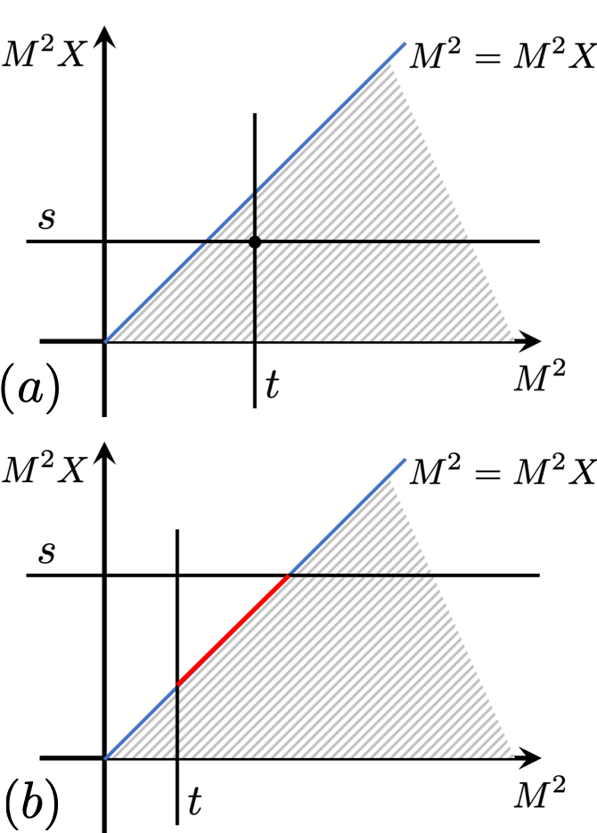
Figure 4: (color online) Locations of classical energy minima of Eq. (121) in the two-dimensional parameter space subtended by $M^{2}$ and $M^{2}x$ $(<M^{2})$. (a) $h<h_{c}$ (b) $h>h_{c}$.

When ${\bm{k}}^{\prime}={\bm{k}}^{\prime\prime}$ ($\omega=0$) in Eqs. (105,110), the total classical energy can be further minimized with respect to $A$, $B$ and $\nu$, the angle between ${\bm{\alpha}}^{\prime}$ and ${\bm{\alpha}}^{\prime\prime}$;

$$\frac{1}{\beta V}S[A,B,\nu] =-\Big{(}\alpha-\frac{2}{g}+\frac{D^{2}}{4\lambda}\Big{)}(A^{2}+B^{2})$$

$$-\gamma(A^{2}+B^{2})^{2}+4|\gamma|A^{2}B^{2}\sin^{2}\nu-2hAB\sin\nu.$$

Namely, take $(A,B)\equiv M(\cos\theta,\sin\theta)$, and minimize the energy with respect to $M$ and $x\equiv\sin 2\theta\sin\nu$ $(\leq 1)$,

$$\frac{S}{\beta V} =|\gamma|\big{[}(M^{2}-t)^{2}+(M^{2}x-s)^{2}-(t^{2}+s^{2})\big{]}.$$ (121)

Here $s$ and $t$ are given by

$$t\equiv\frac{h_{c}}{2|\gamma|},\ \ s\equiv\frac{h}{2|\gamma|},\ \ h_{c}\equiv\alpha-\frac{2}{g}+\frac{D^{2}}{4\lambda}.$$ (122)

Since $M^{2}x\leq M^{2}$, the energy has two different minima, depending on whether $s<t$ ($h<h_{c}$) or $s>t$ ($h>h_{c}$). When $h\leq h_{c}$ (Fig. 4(a)), the energy has a minimum at

$$M^{2}=t=\frac{h_{c}}{2|\gamma|},\!\ M^{2}x=s=\frac{h}{2|\gamma|}.$$ (123)

When $h\geq h_{c}$ (Fig. 4(b)), the energy must be minimized along $x=1$. Substituting $x=1$ into Eq. (121), one can see that it has a minimum at

$$M^{2}=\frac{1}{2}(t+s)=\frac{h_{c}+h}{4|\gamma|}.$$ (124)

In conclusion, the classical ground state configuration in the presence of the finite in-plane field is characterized by two helicoid orders of ${\bm{\phi}}^{\prime}_{c}({\bm{x}})$ and ${\bm{\phi}}^{\prime\prime}_{c}({\bm{x}})$. When the in-plane field is along the $+x$-direction, they take the following forms. For $h<h_{c}$,

$$\left\{\begin{array}[]{c}{\bm{\phi}}^{\prime}_{c}({\bm{x}})=\rho\cos\theta\big{(}\cos(Ky){\bm{e}}_{y}-\sin(Ky){\bm{e}}_{z}\big{)}\\ {\bm{\phi}}^{\prime\prime}_{c}({\bm{x}})=\rho\sin\theta\big{(}\cos(Ky-\nu){\bm{e}}_{y}-\sin(Ky-\mu){\bm{e}}_{z}\big{)}\\ K=\frac{D}{2\lambda},\!\ \!\ \rho=\sqrt{\frac{h_{c}}{2|\gamma|}},\!\ \!\ \sin\nu\sin 2\theta=\frac{h}{h_{c}}\\ \end{array}\right..$$ (128)

For $h>h_{c}$,

$$\left\{\begin{array}[]{c}{\bm{\phi}}^{\prime}_{c}({\b{x}})+i{\bm{\phi}}^{\prime\prime}_{c}({\bm{x}})=e^{iKy}\frac{\rho^{\prime}}{\sqrt{2}}({\bm{e}}_{y}+i{\bm{e}}_{z})\\ K=\frac{D}{2\lambda},\!\ \!\ \rho^{\prime}=\sqrt{\frac{h_{c}+h}{4|\gamma|}}\\ \end{array}\right..$$ (131)

Appendix C derivation of linearized EOM for fluctuation of the spin-1 exciton field

In this appendix, we derive a linearized equation of motion (EOM) for a fluctuation of the spin-1 exciton field around the helicoidal structure (Eqs. (128,131)). We first take a functional derivative of the effective action (Eq. (4)), to derive a coupled nonlinear EOMs for real and imaginary parts of the spin-1 exciton field;

$$|\eta|\partial_{t}\phi^{\prime\prime}_{x} -\Big{(}\alpha-\frac{2}{g}\Big{)}\phi^{\prime}_{x}+2|\gamma||{\bm{\phi}}^{\prime}|^{2}\phi^{\prime}_{x}+6|\gamma||{\bm{\phi}}^{\prime\prime}|^{2}\phi^{\prime}_{x}-4|\gamma|({\bm{\phi}}^{\prime}\cdot{\bm{\phi}}^{\prime\prime})\phi^{\prime\prime}_{x}+D\partial_{x}\phi^{\prime}_{z}-\lambda{\bm{\nabla}}^{2}\phi^{\prime}_{x}=0,$$

$$-|\eta|\partial_{t}\phi^{\prime}_{x} -\Big{(}\alpha-\frac{2}{g}\Big{)}\phi^{\prime\prime}_{x}+2|\gamma||{\bm{\phi}}^{\prime\prime}|^{2}\phi^{\prime\prime}_{x}+6|\gamma||{\bm{\phi}}^{\prime}|^{2}\phi^{\prime\prime}_{x}-4|\gamma|({\bm{\phi}}^{\prime}\cdot{\bm{\phi}}^{\prime\prime})\phi^{\prime}_{x}+D\partial_{x}\phi^{\prime\prime}_{z}-\lambda{\bm{\nabla}}^{2}\phi^{\prime\prime}_{x}=0,$$

$$|\eta|\partial_{t}\phi^{\prime\prime}_{y} -\Big{(}\alpha-\frac{2}{g}\Big{)}\phi^{\prime}_{y}+2|\gamma||{\bm{\phi}}^{\prime}|^{2}\phi^{\prime}_{y}+6|\gamma||{\bm{\phi}}^{\prime\prime}|^{2}\phi^{\prime}_{y}-4|\gamma|({\bm{\phi}}^{\prime}\cdot{\bm{\phi}}^{\prime\prime})\phi^{\prime\prime}_{y}+D\partial_{y}\phi^{\prime}_{z}-\lambda{\bm{\nabla}}^{2}\phi^{\prime}_{y}-h\phi^{\prime\prime}_{z}=0,$$

$$-|\eta|\partial_{t}\phi^{\prime}_{y} -\Big{(}\alpha-\frac{2}{g}\Big{)}\phi^{\prime\prime}_{y}+2|\gamma||{\bm{\phi}}^{\prime\prime}|^{2}\phi^{\prime\prime}_{y}+6|\gamma||{\bm{\phi}}^{\prime}|^{2}\phi^{\prime\prime}_{y}-4|\gamma|({\bm{\phi}}^{\prime}\cdot{\bm{\phi}}^{\prime\prime})\phi^{\prime}_{y}+D\partial_{y}\phi^{\prime\prime}_{z}-\lambda{\bm{\nabla}}^{2}\phi^{\prime\prime}_{y}+h\phi^{\prime}_{z}=0,$$

$$|\eta|\partial_{t}\phi^{\prime\prime}_{z} -\Big{(}\alpha-\frac{2}{g}\Big{)}\phi^{\prime}_{z}+2|\gamma||{\bm{\phi}}^{\prime}|^{2}\phi^{\prime}_{z}+6|\gamma||{\bm{\phi}}^{\prime\prime}|^{2}\phi^{\prime}_{z}-4|\gamma|({\bm{\phi}}^{\prime}\cdot{\bm{\phi}}^{\prime\prime})\phi^{\prime\prime}_{z}-D{\bm{\nabla}}\cdot{\bm{\phi}}^{\prime}-\lambda{\bm{\nabla}}^{2}\phi^{\prime}_{z}+h\phi^{\prime\prime}_{y}=0,$$

$$-|\eta|\partial_{t}\phi^{\prime}_{z} -\Big{(}\alpha-\frac{2}{g}\Big{)}\phi^{\prime\prime}_{z}+2|\gamma||{\bm{\phi}}^{\prime\prime}|^{2}\phi^{\prime\prime}_{z}+6|\gamma||{\bm{\phi}}^{\prime}|^{2}\phi^{\prime\prime}_{z}-4|\gamma|({\bm{\phi}}^{\prime}\cdot{\bm{\phi}}^{\prime\prime})\phi^{\prime}_{z}-D{\bm{\nabla}}\cdot{\bm{\phi}}^{\prime\prime}-\lambda{\bm{\nabla}}^{2}\phi^{\prime\prime}_{z}-h\phi^{\prime}_{y}=0,$$

with ${\bm{\nabla}}\equiv(\partial_{x},\partial_{y},0)$. Here we have replaced the imaginary time $\tau$ by the real time $t$; $i\partial_{\tau}=\partial_{t}$. The classical configurations given by Eqs. (128,131) are static solutions of the nonlinear EOMs. We thus introduce a small fluctuation of the exciton field around the classical configuration, ${\bm{\phi}}^{\prime}({\bm{x}})\equiv{\bm{\phi}}^{\prime}_{c}({\bm{x}})+\delta{\bm{\phi}}^{\prime}({\bm{x}})$ and ${\bm{\phi}}^{\prime\prime}({\bm{x}})\equiv{\bm{\phi}}^{\prime\prime}_{c}({\bm{x}})+\delta{\bm{\phi}}^{\prime\prime}({\bm{x}})$ and linearize the EOMs with respect to the fluctuations, $\delta{\bm{\phi}}^{\prime}$ and $\delta{\bm{\phi}}^{\prime\prime}$. For $h\leq h_{c}$, the linearized coupled EOMs for ${\bm{\phi}}^{\dagger}\equiv\delta{\bm{\phi}}^{\prime}-i\delta{\bm{\phi}}^{\prime\prime}$ and ${\bm{\phi}}\equiv\delta{\bm{\phi}}^{\prime}+i\delta{\bm{\phi}}^{\prime\prime}$ are given by

$$i|\eta|\partial_{t}\phi_{x}+\alpha_{\bm{\nabla}}\phi_{x}+2|\gamma|\rho^{2}F_{0}\phi^{\dagger}_{x}-D\partial_{x}\phi_{z}=0,$$

$$i|\eta|\partial_{t}\phi^{\dagger}_{x}-\alpha_{\bm{\nabla}}\phi^{\dagger}_{x}-2|\gamma|\rho^{2}F^{*}_{0}\phi_{x}+D\partial_{x}\phi^{\dagger}_{z}=0,$$

$$i|\eta|\partial_{t}\phi_{y}+\alpha_{\bm{\nabla}}\phi_{y}-(D\partial_{y}-ih)\phi_{z}-C_{y}\phi^{\dagger}_{y}+S_{y}\phi^{\dagger}_{z}=0,$$

$$i|\eta|\partial_{t}\phi^{\dagger}_{y}-\alpha_{\bm{\nabla}}\phi^{\dagger}_{y}+(D\partial_{y}+ih)\phi^{\dagger}_{z}+C^{*}_{y}\phi_{y}-S^{*}_{y}\phi_{z}=0,$$

$$i|\eta|\partial_{t}\phi_{z}+\alpha_{\bm{\nabla}}\phi_{z}+D{\bm{\nabla}}{\bm{\phi}}-ih\phi_{y}+C_{y}\phi^{\dagger}_{z}+S_{y}\phi^{\dagger}_{y}=0,$$

$$i|\eta|\partial_{t}\phi^{\dagger}_{z}-\alpha_{\bm{\nabla}}\phi^{\dagger}_{z}-D{\bm{\nabla}}{\bm{\phi}}^{\dagger}-ih\phi^{\dagger}_{y}-C^{*}_{y}\phi_{z}-S^{*}_{y}\phi_{y}=0.$$

where $\rho$, $\alpha_{\bm{\Delta}}$, $F_{0}$, $C_{y}$, and $S_{y}$ are defined in Eqs. (7,34,36,37,38) respectively. For $h\geq h_{c}$, the linearized EOMs are given by

$$i|\eta|\partial_{t}\phi_{x}+\alpha^{\prime}_{\bm{\nabla}}\phi_{x}-D\partial_{x}\phi_{z}=0,$$

$$i|\eta|\partial_{t}\phi^{\dagger}_{x}-\alpha^{\prime}_{\bm{\nabla}}\phi^{\dagger}_{x}+D\partial_{x}\phi^{\dagger}_{z}=0,$$

$$i|\eta|\partial_{t}\phi_{y}+\alpha^{\prime}_{\bm{\nabla}}\phi_{y}-(D\partial_{y}+ih-i2\zeta)\phi_{z}-\zeta e^{2iKy}(\phi^{\dagger}_{y}+i\phi^{\dagger}_{z})=0,$$

$$i|\eta|\partial_{t}\phi^{\dagger}_{y}-\alpha^{\prime}_{\bm{\nabla}}\phi^{\dagger}_{y}+(D\partial_{y}-ih+i2\zeta)\phi^{\dagger}_{z}+\zeta e^{-2iKy}(\phi_{y}-i\phi_{z})=0,$$

$$i|\eta|\partial_{t}\phi_{z}+\alpha^{\prime}_{\bm{\nabla}}\phi_{z}+D{\bm{\nabla}}{\bm{\phi}}+(ih-2i\zeta)\phi_{y}+\zeta e^{2iKy}(\phi^{\dagger}_{z}-i\phi^{\dagger}_{y})=0,$$

$$i|\eta|\partial_{t}\phi^{\dagger}_{z}-\alpha^{\prime}_{\bm{\nabla}}\phi^{\dagger}_{z}-D{\bm{\nabla}}{\bm{\phi}}^{\dagger}+(ih-2i\zeta)\phi^{\dagger}_{y}-\zeta e^{-2iKy}(\phi_{z}+i\phi_{y})=0.$$

where $\rho^{\prime}$, $\alpha^{\prime}_{\bm{\nabla}}$, and $\zeta$ are defined in Eqs. (13,35,33).

As indicated by the form of the effective action, ${\bm{\phi}}^{\dagger}$ and ${\bm{\phi}}$ play role of spin-1 boson creation and annihilation operator respectively. Therefore, the linearized EOMs should take a form of generalized eigenvalue equation with a bosonic BdG Hamiltonian;

$$|\eta|i\partial_{t}\left(\begin{array}[]{c}\phi_{x}({\bm{x}})\\ \phi_{y}({\bm{x}})\\ \phi_{z}({\bm{x}})\\ \phi^{\dagger}_{x}({\bm{x}})\\ \phi^{\dagger}_{y}({\bm{x}})\\ \phi^{\dagger}_{z}({\bm{x}})\\ \end{array}\right)={\bm{\tau}}_{3}\hat{\bm{H}}_{\rm BdG}({\bm{\nabla}},{\bm{x}})\!\ \left(\begin{array}[]{c}\phi_{x}({\bm{x}})\\ \phi_{y}({\bm{x}})\\ \phi_{z}({\bm{x}})\\ \phi^{\dagger}_{x}({\bm{x}})\\ \phi^{\dagger}_{y}({\bm{x}})\\ \phi^{\dagger}_{z}({\bm{x}})\\ \end{array}\right),$$ (144)

where $\hat{\bm{H}}_{\rm BdG}$ is an Hermitian operator

$$\hat{\bm{H}}^{\dagger}_{\rm BdG}(\partial_{x},\partial_{y},x,y)=\hat{\bm{H}}_{\rm BdG}(-\partial_{x},-\partial_{y},x,y).$$ (145)

In fact, Eq. (145) holds true for eqs. (25,32).

Appendix D evaluation of local magnetic moment and local charge density in the electron layer

In this appendix, we calculate local magnetic moment and local charge density in the electron layer, that are induced by the helicoidal excitonic order ($h<h_{c}$). To this end, let us begin with the following temperature Green’s function fetter03 ,

$$G^{a}_{\alpha\beta}({\bm{x}},\tau;{\bm{x}}^{\prime},\tau^{\prime})=-\frac{{\rm Tr}\big{[}e^{-\beta K}{\cal T}_{\tau}\big{\{}a_{\alpha}({\bm{x}},\tau)a^{\dagger}_{\beta}({\bm{x}}^{\prime},\tau^{\prime})\big{\}}\big{]}}{{\rm Tr}[e^{-\beta K}]}$$ (146)

where

$$a_{\alpha}({\bm{x}},\tau) \equiv e^{K\tau}a_{\alpha}({\bm{x}})e^{-K\tau},$$

$$a^{\dagger}_{\alpha}({\bm{x}},\tau) \equiv e^{K\tau}a^{\dagger}_{\alpha}({\bm{x}})e^{-K\tau},$$

with $K\equiv H_{0}-\mu N+H^{\prime}\equiv K_{0}+H^{\prime}$ and

$$-H^{\prime} =\int d{\bm{x}}\!\ \big{(}{\bm{\phi}}^{\prime}_{c}({\bm{x}})-i{\bm{\phi}}^{\prime\prime}_{c}({\bm{x}})\big{)}{\bm{b}}^{\dagger}({\bm{x}}){\bm{\sigma}}{\bm{a}}({\bm{x}})$$

$$\ \ +\int d{\bm{x}}\!\ \big{(}{\bm{\phi}}^{\prime}_{c}({\bm{x}})+i{\bm{\phi}}^{\prime\prime}_{c}({\bm{x}})\big{)}{\bm{a}}^{\dagger}({\bm{x}}){\bm{\sigma}}{\bm{b}}({\bm{x}}).$$

The classical configuration of the spin-1 exciton field for $h<h_{c}$ is given by Eqs. (9,10). In the momentum space, $K_{0}$ and $H^{\prime}$ are given by

$$K_{0} =\sum_{\bm{k}}a^{\dagger}_{\bm{k}}(\xi^{a}_{\bm{k}}{\bm{\sigma}}_{0}+\xi_{e}(k_{y}{\bm{\sigma}}_{x}-k_{x}{\bm{\sigma}}_{y})+H{\bm{\sigma}}_{x})a_{\bm{k}}$$

$$\ +\sum_{\bm{k}}b^{\dagger}_{\bm{k}}(\xi^{b}_{\bm{k}}{\bm{\sigma}}_{0}+\Delta_{h}(k_{x}{\bm{\sigma}}_{x}+k_{y}{\bm{\sigma}}_{y})+H{\bm{\sigma}}_{x})b_{\bm{k}}$$

$$H^{\prime} =-\frac{\rho}{2}\sum_{{\bm{k}}_{1},{\bm{k}}_{2}}\!$$

$$\Big{\{}{\bm{b}}^{\dagger}_{{\bm{k}}_{1}}({\bm{\sigma}}_{y}+i{\bm{\sigma}}_{z}){\bm{a}}_{{\bm{k}}_{2}}\delta_{{\bm{k}}_{1},{\bm{k}}_{2}+K{\bm{e}}_{y}}\big{(}\cos\theta-ie^{-i\nu}\sin\theta\big{)}$$

$$+{\bm{b}}^{\dagger}_{{\bm{k}}_{1}}({\bm{\sigma}}_{y}-i{\bm{\sigma}}_{z}){\bm{a}}_{{\bm{k}}_{2}}\delta_{{\bm{k}}_{1},{\bm{k}}_{2}-K{\bm{e}}_{y}}\big{(}\cos\theta-ie^{i\nu}\sin\theta\big{)}$$

$$+{\bm{a}}^{\dagger}_{{\bm{k}}_{1}}({\bm{\sigma}}_{y}+i{\bm{\sigma}}_{z}){\bm{b}}_{{\bm{k}}_{2}}\delta_{{\bm{k}}_{1},{\bm{k}}_{2}+K{\bm{e}}_{y}}\big{(}\cos\theta+ie^{-i\nu}\sin\theta\big{)}$$

$$+{\bm{a}}^{\dagger}_{{\bm{k}}_{1}}({\bm{\sigma}}_{y}-i{\bm{\sigma}}_{z}){\bm{b}}_{{\bm{k}}_{2}}\delta_{{\bm{k}}_{1},{\bm{k}}_{2}-K{\bm{e}}_{y}}\big{(}\cos\theta+ie^{i\nu}\sin\theta\big{)}\Big{\}},$$

with $\xi^{a/b}_{\bm{k}}\equiv{\cal E}_{a/b}({\bm{k}})-\mu$.

Using the standard Feynman-Dyson perturbation theory fetter03 , we evaluate the temperature Green function up to the lowest order in $H^{\prime}$. Since $H^{\prime}$ connects between electron and hole but it does not between electron and electron or between hole and hole, the lowest order starts from the second order in $H^{\prime}$;

$$G^{a}_{\alpha\beta}({\bm{x}},\tau:{\bm{x}}^{\prime},\tau^{\prime}) =$$

$$\frac{1}{V}\sum_{{\bm{q}},{\bm{q}}^{\prime}}\frac{1}{\beta}\sum_{i\omega_{n}}e^{i{\bm{q}}{\bm{x}}-i{\bm{q}}^{\prime}{\bm{x}}^{\prime}}e^{-i\omega_{n}(\tau-\tau^{\prime})}{G}^{a}_{\alpha\beta}({\bm{q}},{\bm{q}}^{\prime}:i\omega_{n}),$$ (147)

$$G^{a}_{\alpha\beta}({\bm{q}},{\bm{q}}^{\prime}:i\omega_{n}) =\delta_{{\bm{q}}-2K{\bm{e}}_{y},{\bm{q}}^{\prime}}{G}^{a}_{-}({\bm{q}}-K{\bm{e}}_{y},i\omega_{n})$$

$$+\delta_{{\bm{q}},{\bm{q}}^{\prime}}{G}^{a}_{0}({\bm{q}},i\omega_{n})+\delta_{{\bm{q}}+2K{\bm{e}}_{y},{\bm{q}}^{\prime}}{G}^{a}_{+}({\bm{q}}+K{\bm{e}}_{y},i\omega_{n}).$$ (148)

Here

$${G}^{a}_{\mp}({\bm{q}},i\omega_{n}) =\Big{(}\frac{\rho}{2}\Big{)}^{2}(\cos^{2}\theta+e^{\mp i2\nu}\sin^{2}\theta)\!\ {g}^{a}_{0}({\bm{q}}\pm K{\bm{e}}_{y},i\omega_{n})$$

$$({\bm{\sigma}}_{y}\pm i{\bm{\sigma}}_{z}){g}^{b}_{0}({\bm{q}},i\omega_{n})({\bm{\sigma}}_{y}\pm i{\bm{\sigma}}_{z}){g}^{a}_{0}({\bm{q}}\mp K{\bm{e}}_{y},i\omega_{n}),$$

$${G}^{a}_{0}({\bm{q}},i\omega_{n}) =\Big{(}\frac{\rho}{2}\Big{)}^{2}\sum_{\sigma=\pm}(1+\sigma\sin\nu\sin 2\theta)\!\ {g}^{a}_{0}({\bm{q}},i\omega_{n})$$

$$({\bm{\sigma}}_{y}+i\sigma{\bm{\sigma}}_{z}){g}^{b}_{0}({\bm{q}}-\sigma K{\bm{e}}_{y},i\omega_{n})({\bm{\sigma}}_{y}-\sigma i{\bm{\sigma}}_{z}){g}^{a}_{0}({\bm{q}},i\omega_{n}),$$

and

$${g}^{a}_{0}({\bm{q}},i\omega_{n}) =\frac{(i\omega_{n}-\xi^{a}_{\bm{q}}){\bm{\sigma}}_{0}+\xi_{e}(q_{y}{\bm{\sigma}}_{x}-q_{x}{\bm{\sigma}}_{y})+H{\bm{\sigma}}_{x}}{(i\omega_{n}-\xi^{a}_{\bm{q}})^{2}-\big{[}(\xi_{e}q_{x})^{2}+(\xi_{e}q_{y}+H)^{2}\big{]}},$$

$${g}^{b}_{0}({\bm{q}},i\omega_{n}) =\frac{(i\omega_{n}-\xi^{b}_{\bm{q}}){\bm{\sigma}}_{0}+\Delta_{h}(q_{x}{\bm{\sigma}}_{x}+q_{y}{\bm{\sigma}}_{y})+H{\bm{\sigma}}_{x}}{(i\omega_{n}-\xi^{b}_{\bm{q}})^{2}-\big{[}(\Delta_{h}q_{y})^{2}+(\Delta_{h}q_{x}+H)^{2}\big{]}}.$$

The local magnetic moment and charge density in the electron layer is calculated from the Green function,

$$\left\{\begin{array}[]{c}\rho^{e}({\bm{x}})={\rm Tr}\big{[}{G}^{a}({\bm{x}},\tau;{\bm{x}},\tau+0)\big{]}\\ {\bm{m}}^{e}({\bm{x}})=\frac{1}{2}{\rm Tr}\big{[}{\bm{\sigma}}{G}^{a}({\bm{x}},\tau;{\bm{x}},\tau+0)\big{]}\\ \end{array}\right.$$ (151)

When Eqs. (148,147) are substituted into Eq. (151), the first and third terms in Eq. (148) give rise to helicoidal spin density wave in the $yz$ plane, while the second term in Eq. (148) leads to uniform charge density and magnetic moment along the in-plane Zeeman field ($x$-direction). In the leading order in $\Delta_{h}$, they are given by

$$\rho^{e}({\bm{x}}) =C+{\cal O}(\Delta^{2}_{h})$$ (152)

$${\bm{m}}^{e}({\bm{x}}) =A\big{(}\cos^{2}\theta\cos(2Ky)+\sin^{2}\theta\cos(2Ky-2\nu)\big{)}{\bm{e}}_{y}$$

$$-B\big{(}\cos^{2}\theta\sin(2Ky)+\sin^{2}\theta\sin(2Ky-2\nu)\big{)}{\bm{e}}_{z}$$

$$+\frac{1}{2}D{\bm{e}}_{x}+{\cal O}(\Delta^{2}_{h})$$ (153)

where

$$\left(\begin{array}[]{c}A\\ B\\ \end{array}\right) \equiv\frac{\rho^{2}\Delta_{h}}{V}\sum_{\bm{q}}\frac{1}{\beta}\sum_{i\omega_{n}}e^{i\omega_{n}0+}q_{y}f({\bm{q}},H)\left(\begin{array}[]{c}t+s\\ t-s\\ \end{array}\right),$$ (158)

and

$$\left(\begin{array}[]{c}C\\ D\\ \end{array}\right) \equiv\frac{\rho^{2}}{V}\sum_{\bm{q}}\frac{1}{\beta}\sum_{i\omega_{n}}e^{i\omega_{n}0+}\sum_{\sigma=\pm}(1+\sigma\sin\nu\sin 2\theta)$$ (161)

$$\hskip 14.22636pt(i\omega_{n}-\xi^{b}_{\bm{q}}-H)g_{\sigma}({\bm{q}},H)\left(\begin{array}[]{c}u_{\sigma}+s\\ u_{\sigma}-s\\ \end{array}\right),$$ (164)

with

$$f({\bm{q}},H) \equiv\frac{1}{(i\omega_{n}-\xi^{b}_{\bm{q}})^{2}-H^{2}}\prod_{\sigma=\pm}\frac{1}{(i\omega_{n}-\xi^{a}_{{\bm{q}}+\sigma})^{2}-[(\xi_{e}q_{x})^{2}+(\xi_{e}(q_{y}+\sigma K)+H)^{2}]},$$

$$t \equiv[(i\omega_{n}-\xi^{a}_{{\bm{q}}+})+(\xi_{e}(q_{y}+K)+H)][(i\omega_{n}-\xi^{a}_{{\bm{q}}-})-(\xi_{e}(q_{y}-K)+H)],\ \ s\equiv(\xi_{e}q_{x})^{2},$$

$$g_{\sigma}({\bm{q}},H) \equiv\frac{1}{(i\omega_{n}-\xi^{b}_{\bm{q}})^{2}-H^{2}}\bigg{(}\frac{1}{(i\omega_{n}-\xi^{a}_{{\bm{q}}+\sigma})^{2}-[(\xi_{e}q_{x})^{2}+(\xi_{e}(q_{y}+\sigma K)+H)^{2}]}\bigg{)}^{2},$$

$$u_{\sigma} \equiv[(i\omega_{n}-\xi^{a}_{{\bm{q}}+\sigma})+(\xi_{e}(q_{y}+\sigma K)+H)]^{2},$$ (165)

and ${\bm{q}}+\sigma\equiv(q_{x},q_{y}+\sigma K)$ ($\sigma=\pm$). Eqs. (152,153) conclude that up to the first order in $\Delta_{h}$, the helicoidal excitonic order under the in-plane Zeeman field (along $x$) induces the uniform charge density and uniform magnetization (along $x$) as well as the helicoidal magnetic order within the $yz$ plane in the electron layer. A finite uniform charge density induced by the helicoidal excitonic order suggests that the low-energy collective modes in the excitonic phase can couple electrically with external electromagnetic waves. The helicoidal magnetic texture within the $yz$ plane suggests that the helicoidal structure can be seen by the magneto-optical Kerr spectroscopy.

References

- (1) N. F. Mott, Phil. Mag. 6, 287 (1961).
- (2) R. S. Knox, Solid State Physics, edited by F. Seitz and D. Turnbull (Academic Press, New York, 1963), suppl. 5, p. 100.
- (3) L. V. K. Kelydsh, and Y. V. Kopaev, Sov. Phys. Solid State, 6, 2219 (1965).
- (4) D. Jeorme, T. M. Rice, and W. Kohn, Phys. Rev. 158, 462 (1967).
- (5) B. I. Halperin, and T. M. Rice, Rev. Mod. Phys. 40, 755 (1968).
- (6) Y. Wakisaka, T. Sudayama, K. Takubo, T. Mizokawa, M. Arita, H. Namatame, M. Taniguchi, N. Katayama, M. Nohara, and H. Takagi, Phys. Rev. Lett. 103, 026402 (2009).
- (7) A. Kogar, M. S. Rak, S. Vig, A. A. Husain, F. Flicker, Y. I. Joe, L. Venema, G. J. MacDougall, T. C. Chiang, E. Fradkin, J. Wezel, P. Abbamonte, Science 358, 1314 (2017).
- (8) D. Werdehausen, T. Takayama, M. Hoppner, G. Albrecht, A. W. Rost, Y. Lu, D. Manske, H. Takagi, S. Kaiser, Science Advances, 4, eaap8652 (2018).
- (9) Y. E. Lozovik, and Y. I. Yudson, Sov. Phys. JETP Lett. 22, 274 (1975).
- (10) C. Comte, and P. Nozieres, J. Phys. 43, 1069 (1982).
- (11) S. Datta, M. R. Melloch, and R. L. Gunshor, Phys. Rev. B 32, 2607 (1985).
- (12) X. Xia, X. M. Chen, and J. J. Quinn, Phys. Rev. B 46, 7212 (1992).
- (13) X. Zhu, P. B. Littlewood, M. S. Hybertsen, and T. M. Rice, Phys. Rev. Lett. 74, 1633 (1995).
- (14) P. B. Littlewood, and X. Zhu, Physica Scripta T68, 56 (1996).
- (15) Y. Naveh, and B. Laikhtman, Phys. Rev. Lett. 77, 900 (1996).
- (16) A. F. Croxall, K. Das Gupta, C. A. Nicoll, M. Thangaraj, H. E. Beere, I. Farrer, D. A. Ritchie, and M. Pepper, Phys. Rev. Lett. 101, 246801 (2008).
- (17) J. A. Seamons, C. P. Morath, J. L. Reno, and M. P. Lilly, Phys. Rev. Lett. 102, 026804 (2009).
- (18) L. Yang, J. D. Koralek, J. Orenstein, D. R. Tibbetts, J. L. Reno, and M. P. Lilly, Phys. Rev. Lett. 106 247401 (2011).
- (19) U. Sivan, P. M. Solomon, and H. Shtrikman, Phys. Rev. Lett. 68, 1196 (1992).
- (20) X. Wu, W. Lou, K. Chang, G. Sullivan, and R. R. Du, Phys. Rev. B 99, 085307 (2019).
- (21) X. Zhu, M. S. Hybertsen and P. B. Littlewood, Phys. Rev. B 54, 13575 (1996).
- (22) D. I. Pikulin and T. Hyart, Phys. Rev. Lett. 112, 176403 (2014).
- (23) Degeneracy lifting in exciton bands by the SOI was also discussed in monolayer transition metal dichalcogenides; H. Yu, G. B. Liu, P. Gong, X. Xu, and W. Yao, Nature Communications, 5:3876, (2014).
- (24) C. J. Pethick and H. Smith, Bose–Einstein Condensation in Dilute Gases (Cambridge University Press, Cambridge, 2001).
- (25) J. H. Colpa, Physica A 93, 327 (1978).
- (26) A. Hubert, and R. Schafer, Magnetic Domains (Springer-Verlag, Berlin Heidelberg, 1998).
- (27) E. Fradkin, Field Theories of Condensed Matter Systems (Addison-Wesley Publishing Company, Redwood City, 1991).
- (28) A. L. Fetter, and J. D. Walecka, Quantum Theory of Many-Particle Systems (Dover Books, New York, 2003)