Planning under non-rational perception of uncertain spatial costs

Abstract

This work investigates the design of risk-perception-aware motion-planning strategies that incorporate non-rational perception of risks associated with uncertain spatial costs. Our proposed method employs the Cumulative Prospect Theory (CPT) to generate a perceived risk map over a given environment. CPT-like perceived risks and path-length metrics are then combined to define a cost function that is compliant with the requirements of asymptotic optimality of sampling-based motion planners (RRT*). The modeling power of CPT is illustrated in theory and in simulation, along with a comparison to other risk perception models like Conditional Value at Risk (CVaR). Theoretically, we define a notion of expressiveness for a risk perception model and show that CPT’s is higher than that of CVaR and expected risk. We then show that this expressiveness translates to our path planning setting, where we observe that a planner equipped with CPT together with a simultaneous perturbation stochastic approximation (SPSA) method can better approximate arbitrary paths in an environment. Additionally, we show in simulation that our planner captures a rich set of meaningful paths, representative of different risk perceptions in a custom environment. We then compare the performance of our planner with T-RRT* (a planner for continuous cost spaces) and Risk-RRT* (a risk-aware planner for dynamic human obstacles) through simulations in cluttered and dynamic environments respectively, showing the advantage of our proposed planner.

I INTRODUCTION

Motivation

Autonomous robots from industrial manipulators to robotic swarms [1, 2, 3], are becoming less isolated and increasingly more interactive. Arguably, most environments where these robots operate, have an associated spatial cost, which can lead to a robot’s loss or damage. For example, an oily surface can cause a robot to slip and collide with a nearby obstacle, resulting in a crash. In more complex scenarios, a decision maker (DM) may be directly involved with the motion of an autonomous system, such as in robotic surgery, search and rescue operations, or autonomous car driving. The risk perceived from these costs or losses could vary among different DMs. This motivates the consideration of richer models that are inclusive of non-rational perception of spatial costs in motion planning. With this goal, we aim to study how Cumulative Prospect Theory (CPT) [4] can be included into path planning, and compare its paths with those obtained from other risk perception models.

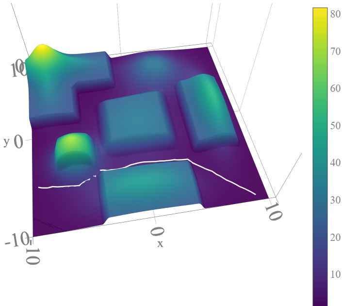
(a) Motion plan with expected risk

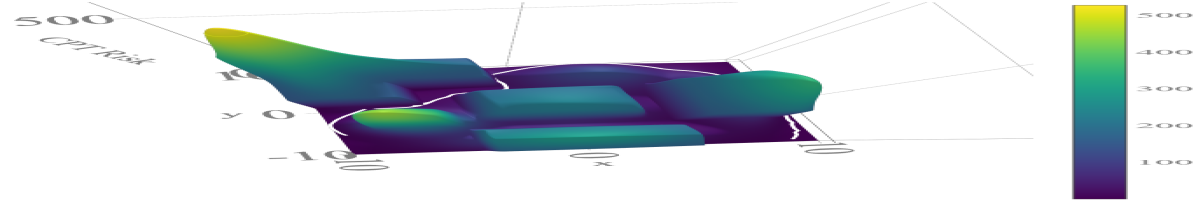
(b) Motion plan with CPT risks

Figure 1: Environment perception and sampling-based motion planning using a) Rational environment perception using expected risk, b) DM’s Risk-Averse environment perception with the chosen path in white.

Related Work

Traditional risk-aware path planning considers risk in the form of motion and state uncertainty [5], collision time [6], or sensing uncertainty [7]. Chance constrained approaches [8, 9] are used to handle agent and environment uncertainty in a robust manner, however discrete polyhedral obstacles are considered which cannot incorporate continuous spatial costs. Stochastic dynamic programming [10] in used in dynamic environments to locally integrate planning and estimation without optimality guarantees. Moreover, in all the above works, how the risks and uncertainties are perceived or relatively weighted has been overlooked. A few recent works [11] contemplate risk perception models, but assume rational DMs and use coherent risk measures like Conditional Value at Risk (CVaR) [12]. Unlike CPT’s suggestions, these measures are built using certain axioms that assume rationality and linearity of the DM’s risk perception [13]. CPT has been extensively used in engineering applications like traffic routing [14], network protection [15], stochastic optimization [16], and safe shipping [17] to model non-rational decision making. However, CPT is yet to be applied in robotic planning and control.

Regarding planning algorithms themselves, RRT* [18] has been the basis for many motion planners due to its asymptotic optimality properties and its ability to solve complex problems [19]. Risk [20] and uncertainty [21] have been an ingredient of motion planning problems involving a human, but have been mainly modeled in a probabilistic manner [22] with discrete obstacles. Very few of these works have considered modeling planning environments via continuous cost maps [23, 24], while, to the best of our knowledge, the simultaneous treatment of cost and uncertainty perception to model a DM’s spatial risk profile has largely been ignored.

Contributions

Our contributions lie in three main areas: Firstly, we adapt CPT into path planning to model non-rational perception of spatial cost embedded in an environment. With this, we can capture a larger variety of risk perception models, extending the existing literature. Secondly, we generate desirable paths using a sampling-based (RRT*-based) planning algorithm on the perceived risky environment. Our planner integrates a continuous risk profile and path length to calculate path cost, enabling us to plan in the perceived environment setting above. Furthermore, the chosen cost satisfies the sufficient conditions for asymptotic optimality of the planner, leading to reliable and consistent paths according to a specified risk profile. We then compare our planner’s performance with T-RRT* (continuous cost space planner) and Risk-RRT* (risk-aware planner) through simulations in cluttered and dynamic environments respectively. We show that our proposed planner can generate better paths in comparison. Finally, we define the notion of “expressiveness” for a risk perception model and show that CPT’s is higher than that of CVaR and expected risk. Furthermore using SPSA, we show that the expressiveness hierarchy translates to our path planning setting, where we observe that a planner equipped with CPT can better approximate arbitrary paths in an environment. We clarify that here, we merely examine CPT based environment perception models for motion planning and leave the validation of these models with human user studies for future work.

Fig. 1 shows a preview of how a nonlinear DM’s perception of the environment influences the path produced to reach a goal. While Fig. 1(a) shows a rational perception of the environment using expected risk, Fig. 1(b) illustrates a nonlinearly deformed and scaled surface that reflects the perception of a certain DM using CPT.

II Preliminaries

Here, we describe some basic notations used in the paper along with a concise description of Cumulative Prospect Theory. More details about CPT can be found in [25].

Notation

We let denote the space of real numbers, $\mathbb{Z}_{\geq 0}$ the space of positive integers and $\mathbb{R}_{\geq 0}$ the space of non negative real numbers. Also, ⁿ and $\mathcal{C}\subset{}^{n}$ denote the $n$-dimensional real vector space and the configuration space used for planning. We use $\|.\|$ for the Euclidean norm and $\circ$ for the composition of two functions $f$ and $g$, that is $f(g(x))=f\circ g(x)$. We model a tree by an directed graph $G=(V,E)$, where $V=\{1,\dots,T\}$ denotes the set of sampled points (vertices of the graph), and $E\subset V\times V$, denotes the set of edges of the graph.

Cost and uncertainty weighting using CPT

CPT is a non-rational decision making model which incorporates non-linear perception of uncertain costs. Traditionally it has been used in scenarios of monetary outcomes such as lotteries [4] and the stock market [25].

Let us suppose a DM is presented with a set of prospects $\{\rho^{1},\dots,\rho^{k},\dots,\rho^{K}\}$, representing potential outcomes and their probabilities, $\rho^{k}=\{(\rho^{k}_{i},p^{k}_{i})\}_{i=1}^{M}$. More precisely, there are $M$ possible outcomes associated with a prospect $k$, given by $\rho_{i}^{k}\in\mathbb{R}_{\geq 0}$, for $i\in\{1,\dots,M\}$, which can happen with a probability $p_{i}^{k}$. The outcomes are arranged in a decreasing order denoted by $\rho_{M}^{k}<\rho_{M-1}^{k}<...<\rho_{1}^{k}$ with their corresponding probabilities, which satisfy $\sum_{i=1}^{M}p_{i}^{k}=1$. The outcomes of prospect $k$ may be interpreted as the random cost of choosing prospect $k$.

We define a utility function, $v:\mathbb{R}_{\geq 0}\rightarrow\mathbb{R}_{\geq 0}$ modeling a DM’s perceived cost and $w:[0,1]\rightarrow[0,1]$ as the probability weighting function which represents the DM’s perceived uncertainty. While previous literature have used various forms for these functions, here we will focus on CPT utility function $v$ taking the form:

$$v(\rho)=\lambda\cdot\rho^{\gamma},$$ (1)

where $0<\gamma<1$ and $\lambda>1$. Tversky and Kahnemann [4] suggest the use of $\gamma=0.88$ and $\lambda=2.25$ to parametrize an average human in the scenario of monetary lotteries, however this may not hold for our application scenario. The parameter $\lambda$ represents the coefficient of cost aversion with greater values implying stronger aversion indicative of higher perceived costs, as indicated in Figure 2(a). The parameter $\gamma$ represents the coefficient of cost sensitivity with lower values implying greater indifference towards cost $\rho$ which is indicated in Figure 2(b).

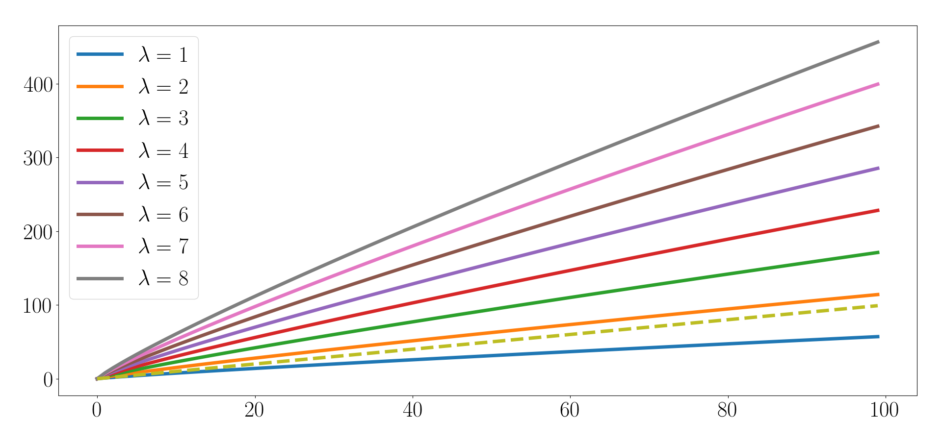
(a) Change in risk aversion $\lambda$ with $\gamma=0.88$

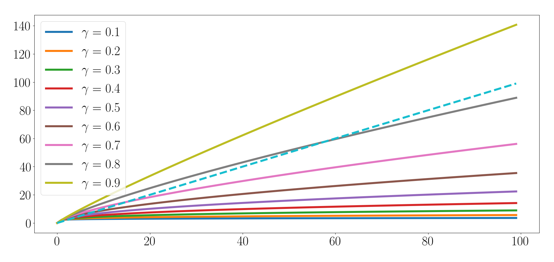
(b) Change in risk sensitivity $\gamma$ with $\lambda=2.25$

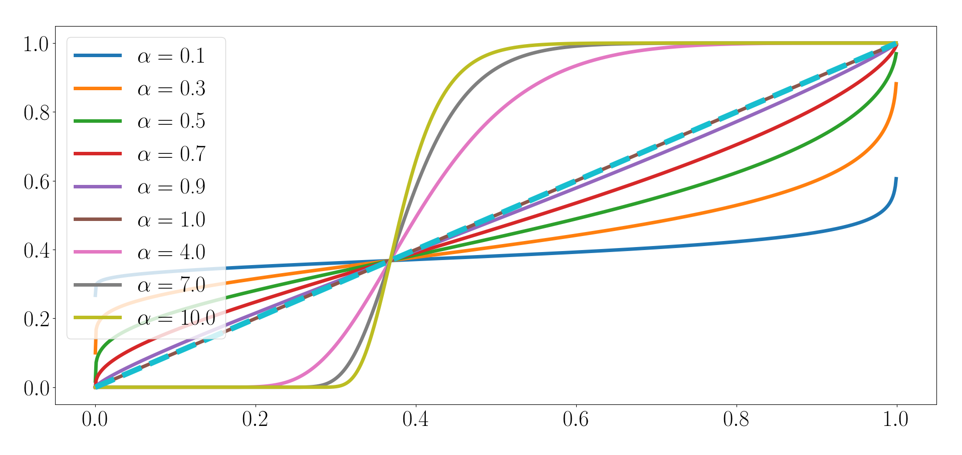
(c) Change in $\alpha$ with $\beta=1$

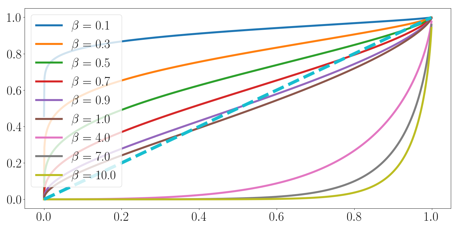
(d) Change in $\beta$ with $\alpha=0.74$

Figure 2: Variation of risk aversion, risk sensitivity and uncertainty perception using CPT. (a)-(b) show risk perception with x-axis indicating the associated risk, $\rho$, and the y-axis showing the perceived risk, $v$. The dotted line indicates the line $v=\rho$. (c)-(d) show uncertainty perception with x-axis indicating probabilities $p$ and y-axis showing their perception $w$, with the dotted line depicting $w=p$

We will be using the popular Prelec’s probability weighting function [25, 26] indicative of perceived uncertainty, which takes the form:

$$w(p)=e^{-\beta(-\log p)^{\alpha}},\alpha>0,\beta>0,w(0)=0.$$ (2)

Figures 2(c) and 2(d) show changing uncertainty perception resulting from varying $\alpha$ and $\beta$ respectively. By choosing low $\alpha$ and $\beta$ values, one can get “uncertainty averse” behavior with $w(p)>p$, implying that unlikely outcomes are perceived to be more certain, as seen on Figures 2(c) and 2(d). When $w(p)<p$, “uncertainty insensitive” behavior is obtained implying that the DM only considers more certain outcomes, which can be observed with high $\alpha$ and $\beta$ values.

These concepts illustrate the nonlinear perception of cost and uncertainty, a DM under consideration can be categorized by the parameters $\Theta=\{\alpha,\beta,\gamma,\lambda\}$. Using the non-linear parametric perception functions $v$ and $w$, CPT calculates a value function $R^{c}(\rho)$, indicating the perceived risk value of the prospect $\rho$. This calculation is detailed in Section IV using our planning setting.

III Environment Setup and Problem Statement

In this work, we consider spatial sources of risk embedded in the $\mathcal{C}$ space. Our starting point is an uncertain cost function $\rho(x)$ that aims to quantify objectively the (negative) consequences of being at a location $x$ or adopting a certain decision under uncertainty at a point $x$.

For example, suppose a robot moves to a location $x$ from $x^{\prime}$ where there is an obstacle with certain probability. Then, we can define a cost measurement as the possible damage to the robot by moving from $x^{\prime}$ to $x$ under action $a^{\prime}$ applied at $x^{\prime}$. A cost value $\rho(x^{\prime},x,a^{\prime})$ can be defined depending on i) the type of robot (flexible robot or rigid robot), ii) the probability of having an obstacle in the said location, and iii) the type of action applied at $x^{\prime}$ to get to $x$ (e.g. slow/fast velocity). For simplicity, adopting a worst-case scenario, we may reduce the previous cost function to a function of the state $\rho(x)\equiv\max_{x^{\prime},a^{\prime}}\rho(x^{\prime},x,a^{\prime})$.

As another example, consider a drone navigating in a building which is ablaze. In this case, the cost function can be proportional to the temperature profile. As sensors are noisy, the temperature profile is uncertain, resulting into a noisy spatial cost value $\rho(x)$. Similarly, environmental conditions that affect the robot’s motion may lead to underperformance. When moving over an icy road, the dynamics of the robot may behave unpredictably, resulting in a temporary loss of control and departure from an intended goal state. In this case, the uncertain cost may be quantified as the state disturbance under a given action over a given period of time. For example, for a simple second-order and fully actuated vehicle dynamics with acceleration input $a$ which is subject to a locally constant “ice” disturbance $d(x)\approx d$, in a small neighborhood of $x$, we have $(x^{\prime}-x)=(a+d(x))\Delta t^{2}/2$ for a small time $\Delta t$. Thus, the difference with an intended state can be measured by the random variable $\rho(x)=\frac{\|d(x)\|\Delta t^{2}}{2}$, which encodes information about $d(x)$ and the unit time of actuation, $\Delta t$. Here $d(x)$ is uncertain, and can be modeled with prior data or measured with a noisy sensor as in the temperature profile case.

Prior knowledge in the form of expert inputs and data collected from sensors can be used to get information about the cost $\rho(x)$, environmental uncertainty, and the robot’s capabilities. In this way, icy roads pose much lesser cost in the previous sense to a 4WD car with snow tires than a 2WD car with summer tires, hence the same cost at a given location could be scaled differently depending upon the robot’s capabilities.

In this work, we will assume that the cost at a location $x\in\mathcal{C}$ has been characterized as a random variable $\rho(x)$ with a mean $\rho_{\mu}(x)\in\mathbb{R}_{\geq 0}$ and standard deviation $\rho_{\sigma}(x)\in\mathbb{R}_{\geq 0}$, for each $x\in\mathcal{C}$. We remark that this cost can be constructed from diverse criteria: From nature of location (For eg. operating table at hospital being mostly static but highly risky) to dynamic properties (For eg. velocity, state) of close-by obstacles. In particular, it is reasonable to approximate $\rho_{\mu}(x)$ via a “bump function,” a concept extensively used in differential geometry. To fix ideas, consider the previous case where a vehicle moves through an “icy” environment, and assume $\Delta t=1$. Then, a mean disturbance over a subset $A\subseteq\mathcal{C}$ should result approximately into a disturbance $\frac{\|d\|}{2}\ell=\rho^{\textup{max}}\ell$, where $\ell$ is the portion of the trajectory from $x$ to $x^{\prime}$ that is inside the icy section $A$. As $x$ is farther from $x^{\prime}$, the disturbance reduces its effect on $x$, and the value of $\ell$ should decrease to zero. In other words, there is a $B$ such that $A\subseteq B$, where $B$ is an enlarged region whose boundary delimits the uncertain cost area from the certain one (i.e. outside $B$ the cost is zero with low uncertainty). The effect of $\ell$ is thus similar to that of a bump function defined with respect to $A$ and $B$. Bump functions are infinitely smooth, take a positive constant value over $A$, which smoothly decreases and becomes zero outside $B$. There are many ways of defining bump functions on manifolds, such as via convolutions, which works in arbitrary dimensions as described the following. Let $\chi_{D}:\mathcal{C}\rightarrow\real$ denote the indicator function of a subset $D\subseteq\mathcal{C}$, and, given $A$, define $f(x)=\frac{\rho^{\textup{max}}}{C}\exp(-\frac{1}{1-\|x\|^{2}})\chi_{A}(x)$, with $\int_{A}\exp(-\frac{1}{1-\|x\|^{2}})=C$. Then, a bump function based on $A$ and $B$ can be given by the convolution $b(x)=\chi_{B}\star f(x)$, $x\in\mathcal{C}$. This function takes a value of $0$ outside $B$, $\rho^{\textup{max}}$ inside $A$ and a value between $0$ and $\rho^{\textup{max}}$ at the points $x\in B\setminus A$. See Section VII for an alternative choice of bump function.

In this work, the notions of “risk” and “risk perception” relate to the way in which the values of $\rho(x)$ are scaled and averaged in expectation. That is, risk is a moment of a given uncertain function (either $\rho(x)$ or a composition with $\rho$). For example, the risk of being at a location $x$ can be measured via expected cost; that is $R^{e}(x)=\mathbb{E}(\rho(x))$, which may represent “expected damage to robot” with respect to uncertainty. However, there are other ways of weighting the $\rho(x)$ outcomes to define alternative risk functions, such as using CPT. With this is mind, we proceed to define the following three main problems and address them in Section IV, Section V and Section VI, respectively.

Problem 1

(CPT environment generator). Given the configuration space $\mathcal{C}$ containing the uncertain cost $\rho$ along with the DM’s CPT parameters $\Theta$, obtain a DM’s (non-rational) perceived risk $R^{c}$ consistent with CPT theory.

Problem 2

(Planning with perceived risk). Given a start and goal points $x_{s}$ and $x_{g}$, compute a desirable path $P$ from $x_{s}$ to $x_{g}$ in accordance with the DM’s perceived risk $R^{c}$.

Problem 3

(CPT planner evaluation). Given a configuration space $\mathcal{C}$, and an uncertain cost $\rho$ along with a drawn path $P_{d}$, evaluate the CPT planner as a model approximator to generate the perceived risk $R^{c}$ representing the path $P_{d}$.

IV Risk perception using CPT

Here, we will generate a DM’s perceived risk and address Problem 1. We consider an uncertain cost $\rho(x)$ is given at every point $x\in\mathcal{C}$, which we approximate via its first two moments, a mean value $\rho_{\mu}(x)\in\mathbb{R}_{\geq 0}$ and a standard deviation $\rho_{\sigma}(x)\in\mathbb{R}_{\geq 0}$. In what follows, we use a discrete approximation of $\rho(x)$ by considering $M\in\mathbb{Z}_{\geq 0}$ bins, to obtain a set of possible cost values $\rho(x)\triangleq\{\rho_{1}(x),\dots,\rho_{M}(x)\}$ such that $\rho_{M}(x)<\rho_{M-1}(x)<...<\rho_{1}(x)$ with their corresponding probabilities $p(x)\triangleq\{p_{1}(x),\dots,p_{M}(x)\}$, such that $\sum_{i=1}^{M}p_{i}(x)=1\ \forall x\in\mathcal{C}$. Further, we will assume that $p_{i}(x_{1})=p_{i}(x_{2})\equiv p_{i},\ \ \forall x_{1},\ x_{2}\in\mathcal{C}\ ,\mbox{and}\ i\in\{1,...,M\}$. In other words, even though cost values $\rho_{i}(x)$, $i\in\{1,\dots,M\}$, may change from point to point in $\mathcal{C}$, the probabilities $p_{i}(x)$ remain the same for different $x$. Note that we can do this wlog by discretizing the continuous RV appropriately, see Algorithm 1. The function $discretize$ finds $y_{i}(x)<y_{i+1}(x)$ such that $\mathbb{P}[y_{i}(x)\leq\rho(x)\leq y_{i+1}(x)]=p_{i+1}(x)-p_{i}(x)$.

Now, the expected Risk $R^{e}(x)$ at a point $x$ is

$$R^{e}(x)\triangleq\sum_{i=1}^{M}\rho_{i}(x)p_{i}(x).$$ (3)

That is, from (3) we have an expected risk $R^{e}:\mathcal{C}\rightarrow\mathbb{R}_{\geq 0}$ defined over $\mathcal{C}$ which is shown in Figure 1(a) and corresponds to a standard or rational notion of risk.

Next, we use the CPT notions developed in Section II to provide a non-rational perception model of the cost $\rho(x)$. According to CPT [4], there is a notion of cumulative functions $\Pi:=\{\pi_{1},...,\pi_{M}\}$ used to non-rationally modify the perception of the probabilities $p_{i}(x)$ in a cumulative fashion. Defining a partial sum function $S_{j}(p_{1},\dots,p_{M})\triangleq\sum_{i=j}^{M}p_{j}$ we have

$$\pi_{j}=w\circ S_{j}(p_{1},\dots,p_{M})\\ -w\circ S_{j+1}(p_{1},\dots,p_{M}),$$ (4)

where we employ the weighting function $w$ from (2).

With this, a DM’s CPT risk $R^{c}:\mathcal{C}\rightarrow\mathbb{R}_{\geq 0}$ associated to the configuration space is given by:

$$R^{c}(x)\triangleq\sum_{j=1}^{M}(v\circ\rho_{j}(x))(\pi_{j}\circ p(x)).$$ (5)

We note that both functions $R^{e}$ and $R^{c}$ are differentiable, which is important for the good behavior of the planner and which will be used for the analysis in Section V.

1Input: $\rho_{\mu}(x),\ \rho_{\sigma}(x),\ \Theta,\ \{p_{1},...,p_{M}\}$

2 Output : $R^{c}(x)$

3 for $i\in\{1,...,M\}$ do

4       $y_{i}(x),y_{i+1}(x)\leftarrow discretize(p_{i}(x),p_{i+1}(x))$;

5       $\rho_{i}(x)\leftarrow\frac{y_{i+1}(x)-y_{i}(x)}{2}$;

6      

7 end for

8$w\circ p(x)\leftarrow e^{-\beta(-\log\circ p(x))^{\alpha}}$ ;

9 $v\circ\rho(x)\leftarrow\lambda(\rho(x))^{\gamma}$ ;

10 for $j\in\{1,...,M\}$ do

11       $\pi_{j}\leftarrow w\circ S_{j}(p_{1},\dots,p_{M})-w\circ S_{j+1}(p_{1},\dots,p_{M})$ ;

12      

13 end for

14$R^{c}(x)\leftarrow\sum_{j=1}^{M}(v\circ\rho_{j}(x))(\pi_{j}\circ p(x))$ ;

15

Algorithm 1 CPT Environment (CPT-Env)

The above concepts are illustrated in Figure 1. Given an uncertain spatial cost $\rho$ with the first moment $\rho_{\mu}$ (Figure 4(b)) and second moment $\rho_{\sigma}$ (Figure 4(c)) across an environment, the DM’s perception can vary from being rational (i.e. using expected risk $R^{e}$ in Figure 1(a)) to non-rational (i.e using CPT risk $R^{c}$). By varying $\Theta$, CPT risk $R^{c}$ can be tuned to represent risk averse (Figure 1(b)), risk indifferent (Figure 4(d)) perception, as well as uncertainty indifferent (Figure 4(e)) to uncertainty averse (Figure 4(f)) perception.

This process gives us the CPT perceived risk at a point $x$, the process is summarized in Algorithm 1. It can be seen that Algorithm 1 does not depend on the dimensionality of the $\mathcal{C}$ space, but on the discretization factor $M$. We will now use the perceived environment for planning in the next section.

V Sampling-based Planning using perceived risk

Here, we will use CPT notions to derive new cost functions, which will be used for planning in the DM’s perceived environment generated in Section IV. In traditional RRT* optimal planning is achieved using path length as the metric. In our setting, the notion of path length is insufficient as it does not capture the risk in $\mathcal{C}$. Thus, we define cost functions that a) take into account risk and path length of a path, and b) satisfy the requirements that guarantee the asymptotic performance of an RRT*-based planner.

Path costs functions

Let two points $x,y\in\mathcal{C}$ be arbitrarily close. A decrease in risk is a desirable trait, hence it is reasonable to add an additional term in the cost only if $R(y)-R(x)\geq 0$, which indicates an increase in DM’s perceived risk by traveling from $x$ to $y$. Consider the set of parameterized paths $\mathcal{P}(\mathcal{C})\triangleq\{\eta:[0,1]\rightarrow\mathcal{C}\;|\;\eta(0)=x,\,\eta(1)=y\}$. First, we first define the cost $J^{c}:\mathcal{P}(\mathcal{C})\rightarrow\mathbb{R}_{\geq 0}$ of a path $\eta\in\mathcal{P}(\mathcal{C})$. Consider a discretization of $[0,1]$ given by $\{0,t_{1},t_{2},\dots,t_{L}=1\}$ with $t_{\ell+1}-t_{\ell}=\Delta t$, for all $\ell$. Then, a discrete approximation of the cost over $\eta$ should be:

$$J^{c}(\eta)\approx\Delta t\sum_{\ell=1}^{L}\max\{0,\frac{R^{c}(\eta(t_{\ell+1}))-R^{c}(\eta(t_{\ell}))}{\Delta t}\}+\delta L(\eta),$$

where $L(\eta)$ denotes the arc-length of the curve $\eta$, and $\delta\in\mathbb{R}_{\geq 0}$ is a constant encoding an urgency versus risk tradeoff. The greater the $\delta$ value, the greater is the urgency and hence path length is more heavily weighted whereas, smaller $\delta$ indicates greater prominence towards risk. The choice of $\delta$ will be discussed in Section VII. By taking limits in the previous expression, and due to the continuity and integrability of $\max$, we can express $J^{c}(\eta)$ as:

$$J^{c}(\eta)= \lim_{\Delta t\rightarrow 0}\Delta t\sum_{\ell=1}^{L}\max\{0,\frac{R^{c}(\eta(t_{\ell+1}))-R^{c}(\eta(t_{\ell}))}{\Delta t}\}+\delta L(\eta)$$

$$=\int_{0}^{1}\max\{0,\frac{d}{dt}(R^{c}(\eta(t))\}\text{d}t+\delta L(\eta)=$$

$$\int_{0}^{1}\max\{0,(R^{c})^{\prime}(\eta(t))\cdot\eta^{\prime}(t)\}\text{d}t+\delta L(\eta).$$ (6)

From here, the cost of traveling from $x$ to $y$ is given by

$$J^{c}(x,y)\triangleq\min_{\eta\in\mathcal{P}(\mathcal{C}):\eta(0)=x,\eta(1)=y}J^{c}(\eta).$$

Similarly, the path cost using expected risk $J^{e}:\mathcal{P}(\mathcal{C})\rightarrow\mathbb{R}_{\geq 0}$ can be obtained by replacing the CPT cost $R^{c}$ in (6) with the expected risk $R^{e}$ as calculated in (3).

Remark 1

(Monotonicity). It can be verified that the costs $J^{c}$ and $J^{e}$ satisfy monotonic properties in the sense that 1) they assign a positive cost to any path in $\mathcal{P}(\mathcal{C})$, and 2) given two paths $\eta_{1}$ and $\eta_{2}$, and their concatenation $\eta_{2}|\eta_{1}$, in the space $\mathcal{P}(\mathcal{C})$, it holds that $J^{c}(\eta_{1})\leq J^{c}(\eta_{1}|\eta_{2})$ (resp. $J^{e}(\eta_{1})\leq J^{e}(\eta_{1}|\eta_{2})$), (due to the additive property of the integrals) and 3) $J^{c}$ (resp. $J^{e}$) are bounded over a bounded $\mathcal{C}$.

1Input: $T,x_{s},x_{g}\$; Output : $G(V,E),P$

2 $V\leftarrow x_{s}$, $E\leftarrow\phi$, $J_{\textup{cum}}^{c}(x_{s})\leftarrow 0$;

3 for $i\in\{1,\dots,T\}$ do

4       $G\leftarrow(V,E)$; $x_{\textup{rand}}\leftarrow Sample()$;

5       $x_{\textup{nearest}}\leftarrow Nearest(G,x_{\textup{rand}})$; $x_{\textup{new}}\leftarrow Steer(x_{\textup{nearest}},x_{\textup{rand}})$;

6       $V\leftarrow V\cup{x_{\textup{new}}}$; $x_{\textup{min}}\leftarrow x_{\textup{nearest}}$;

7       $X_{\textup{near}}\leftarrow Near(G,x_{\textup{new}},\gamma_{\textup{RRT*}},d)$;

8       $c_{\textup{min}}\leftarrow J_{\textup{cum}}^{c}(x_{\textup{nearest}})+J^{\textup{c}}(x_{\textup{nearest}},x_{\textup{new}})$ ;

9       for $x_{\textup{near}}\in X_{\textup{near}}$ do

10             $c^{\prime}\leftarrow J_{\textup{cum}}^{c}(x_{\textup{near}})+J^{c}(x_{\textup{near}},x_{\textup{new}})$;

11             if $c^{\prime}<c_{min}$ then

12                   $x_{\textup{min}}\leftarrow x_{\textup{near}}$; $c_{\textup{min}}\leftarrow c^{\prime}$ ;

13                  

14             end if

15            

16       end for

17      $J_{\textup{cum}}^{c}(x_{\textup{new}})\leftarrow c_{\textup{min}}$ ; $E\leftarrow E\bigcup(\{x_{\textup{near}},x_{\textup{new}}\})$;

18       for $x_{\textup{near}}\in X_{\textup{near}}$ do

19             $c^{\prime}\leftarrow J_{\textup{cum}}^{c}(x_{\textup{new}})+J^{c}(x_{\textup{new}},x_{\textup{near}})$;

20             if $c^{\prime}<J_{\textup{cum}}^{c}(x_{\textup{near}})$ then

21                   $x_{\textup{par}}\leftarrow Parent(x_{\textup{near}},G)$;

22                   $E\leftarrow(E\setminus(\{x_{\textup{par}},x_{\textup{near}}\}))\bigcup(\{x_{\textup{new}},x_{\textup{near}}\})$ ;

23                   $X_{\textup{chld}}\leftarrow Children(x_{\textup{near}},G)$;

24                   for $x_{\textup{chld}}\in X_{\textup{chld}}$ do

25                         $J_{\textup{cum}}^{c}(x_{\textup{chld}})\leftarrow~{}J_{\textup{cum}}^{c}(x_{\textup{chld}})-J_{\textup{cum}}^{c}(x_{\textup{near}})+c^{\prime}$

26                   end for

27                  $J_{\textup{cum}}^{c}(x_{\textup{near}})\leftarrow c^{\prime}$

28             end if

29            

30       end for

31      

32 end for

33$P\leftarrow Path(G,x_{s},x_{g})$ ;

Algorithm 2 CPT-RRT*

Proposed Algorithm

Now we have all the elements to adapt RRT* to our problem setting. Given $\mathcal{C}$, a number of iterations $T$ and a start point $x_{s}\in\mathcal{C}$, we wish to produce graph $G(V,E)$, which represents a tree rooted at $x_{s}$ whose nodes $V$ are sample points in the configuration space and the edges $E$ represent the path between the nodes in $V$. Let $J_{\textup{cum}}^{c}:\mathcal{C}\rightarrow\mathbb{R}_{\geq 0}$ be a function that maps $x\in\mathcal{C}$ to the cumulative cost to reach a point $x$ from the root $x_{s}$ of the tree $G(V,E)$ using the CPT cost metric (6). Similarly we define $J_{\textup{cum}}^{e}:\mathcal{C}\rightarrow\mathbb{R}_{\geq 0}$ for the expected cost function $J^{e}$.

Remark 2

(Additivity). The cumulative costs $J_{\textup{cum}}^{h}$ and $J_{\textup{cum}}$ are additive with respect to costs $J^{c}$ and $J^{e}$ in the sense that: for any $x\in V$ we have $J_{\textup{cum}}^{c}(x)=J_{\textup{cum}}^{c}(Parent(x))+J^{c}(Parent(x),x)$ and similarly $J_{\textup{cum}}^{c}(x)=J_{\textup{cum}}^{e}(Parent(x))+J^{c}(Parent(x),x)$.

The other basic functional components of our algorithm CPT-RRT* (Algorithm 2) are similar to RRT*, and we briefly outline it out here for the sake of completeness:

• $Sample()$: Returns a pseudo-random sample $x\in\mathcal{C}$ drawn from a uniform distribution across $\mathcal{C}$. Other risk-averse sampling schemes as in [23] may be employed. However, such schemes lead to conservative plans, which may not be suitable for all risk profiles.

• $Nearest(G,x)$: Returns the nearest node according to the Euclidean distance metric from $x$ in tree $G$.

• $Steer(x_{1},x_{2})$ returns

  $$\begin{cases}x_{2},&\text{if $\|x_{2}-x_{1}\|\leq d$}\\ x_{1}+d\frac{x_{2}-x_{1}}{\|x_{2}-x_{1}\|},&\text{otherwise.}\end{cases}$$

• $Near(G,x,\gamma_{RRT^{*}},d)$: returns a set of nodes $X\in V$ around $x$, which are within a radius as given in [18].

• $Parent(x,G)$: Returns the parent node of $x$ in the tree $G$.

• $Children(x,G)$: Returns the list of children of $x$ in $G$.

• $Path(G,x_{s},x_{g})$: Returns the path from the nearest node to $x_{g}$ in $G$ to $x_{s}$.

We note that in order to compute $J^{c}$ for each path, we approximate the cost as the sum of costs over its edges, $(x_{1},x_{2})$, and for each edge we compute the cost as the differences $\max\{0,R^{c}(x_{2})-R^{c}(x_{1})\}+\delta L(x_{1},x_{2})$, where the latter is just the length of the edge. Then, this approximation will approach the computation of the real cost in the limit as the number of samples goes to infinity. The values $R^{c}$ are evaluated according to Algorithm 1. Our proposed CPT-RRT* algorithm augments RRT* algorithm in the following aspects: we consider a general continuous cost profile which leads to no obstacle collision checking. We also consider both path length and CPT costs for choosing parents and rewiring with the parameter $\delta$ which serves as relative weighting between CPT costs and Euclidean path length.

Remark 3

(ER-RRT*). We can obtain the expected risk version of Algorithm 2 by replacing cost function $J^{c}$ by $J^{e}$ and following the same procedure as Algorithm 2.

Lemma 1

(Asymptotic Optimality). Assuming compactness of $\mathcal{C}$ and the choice of $\gamma_{RRT^{*}}$ according to Theorem 38 in [18] , the CPT-RRT* algorithm is asymptotically optimal.

Proof:

It follows from the application of Theorem 38 in [18], and the conditions required for the result to hold. More precisely, the cost functions are monotonic (which follows from Remark 1), it holds that $c(\eta)=0$ iff $\eta$ reduces to a single point (resp. the same for $c$), and the cost of any path is bounded. The latter follows from the compactness of $\mathcal{C}$ and continuity of the cost functions. In addition, the costs are also cumulative, due to the additivity property in Remark 2. Finally, the result also requires the condition of the zero measure of the set of points of an optimal trajectory. This holds because both costs include a term for path length. ∎

Simulation results of CPT-RRT* algorithm are presented in Section VII-A. Next we describe our proposed method to evaluate and compare risk perception models in our setting.

VI CPT-planner parameter adaptation

In this section, we theoretically compare CPT value function with other risk perception functions and we describe an algorithm that can adapt the CPT parameters of the planner to approximate arbitrary paths in the environment. By doing so, we aim to evaluate the expressive power of the CPT risk perception model, both theoretically and in a motion planner by comparing its capability to approximate single and arbitrary paths in the environment versus other approaches using different risk perception models.

If successful, this method could be used as a first ingredient in a larger scheme aimed at learning the risk function of a human decision maker using techniques such as inverse reinforcement learning (IRL). We recall that IRL requires either discrete state and action spaces or, if carried out over infinite-dimensional state and action spaces, a class of parameterized functions that can be used to approximate system outputs. Since our planning problem is defined over a continuous state and action space, the class of CPT planners for a parameter set could play the role of a function approximation class required to apply IRL. Then, as is done in IRL, a larger collection of path examples can used to learn the best weighted combination of specific CPT planners in the class. While certainly of interest, this IRL question is out of the scope of this work, and we just focus on analyzing the expressive power of the proposed class of CPT planners. Having a good expressive power is a necessary prerequisite for the class of CPT planners to constitute a viable function approximation class. Firstly, we will define the notion of expressiveness and compare the expressiveness risk perception models from a theoretical point of view. Next, we will describe an approach to compare expressiveness in a path planning setting using SPSA.

VI-A Expressiveness for a risk perception model.

Let $\rho$ be a random cost variable with an associated probability distribution. Let $R$ be a risk value function (with $R(\rho)\in\mathbb{R}_{\geq 0}$) which associates a real value to the random cost variable $\rho$. We can compare the expressiveness of two risk perception models by comparing the range space of their respective risk value functions.

Definition 1

(Expressiveness). Consider two risk perception models $\mathcal{M}_{1}$ and $\mathcal{M}_{2}$ with corresponding classes of risk value functions $\mathcal{V}_{1}$ and $\mathcal{V}_{2}$ with respective range spaces $\mathcal{R}_{1}$ and $\mathcal{R}_{2}$. We say that $\mathcal{M}_{1}$ is more expressive ($\geqq$) than $\mathcal{M}_{2}$ if $\mathcal{R}_{2}\subseteq\mathcal{R}_{1}$ for any given positive random variable $\rho$. That is,

$$\mathcal{M}_{1}\geqq\mathcal{M}_{2}\iff\{R_{2}(\rho)|R_{2}\in\mathcal{V}_{2}\}\subseteq\{R_{1}(\rho)|R_{1}\in\mathcal{V}_{1}\}$$

With this definition, we can compare expressivity of CPT with Conditional Value at Risk (CVaR) [13], also known as “expected shortfall”, another popular risk perception model in the financial decision making community. CVaR uses a single parameter $q\in[0,1)$ representing the fraction of worst case outcomes to consider for evaluating expected risk of an uncertain cost $\rho$. We will use $R^{v}_{Q}$ to denote the perceived risk by CVaR model with $q=Q$. So a $q\approx 1$ considers the worst case outcome of $\rho$ and a $q=0$ considers all the outcomes thus making the CVaR value equal to expected risk ($R^{v}_{0}=R_{E}$). Now we will proceed to compare expressiveness of Expected Risk, CVaR and CPT with parametrized risk value function classes $R^{e}$, $R^{v}$ and $R^{c}$ respectively.

Proposition 1

Let us Consider Expected risk (ER), CVaR and CPT risk models with risk value function classes $R^{e}$, $R^{v}$ and $R^{c}$ defined accordingly. Then, Expected Risk is the least expressive of the three models, that is $\text{CVar}\geqq\text{ER}$ and $\text{CPT}\geqq\text{ER}$ for any given random variable $\rho$.

Proof:

The function class $R^{e}$ has a single function $\mathbb{E}(\rho)$ which gives the expected value of $\rho$. So the range set of $R^{e}$ is a singleton, containing the expected value of $\rho$. It is easy to see that by choosing a function $R^{v}_{0}\in R^{v}$ and $R^{c}_{\overline{\Theta}}\in R^{c}$ where $\overline{\Theta}=\{1,1,1,1\}$ we have $R^{v}_{0}(\rho)=R^{e}(\rho)=R^{c}_{\overline{\Theta}}$. Which implies that $\mathbb{E}(\rho)\in\{R^{v}_{q}(\rho)|q\in[0,1)\}$ and also $\mathbb{E}(\rho)\in\{R^{c}_{\Theta}(\rho)|R^{c}_{\Theta}\in R^{c}\}$, thus proving the expressive order. ∎

Next we will look at the relationship between the CVaR value of a random variable $\rho$ and the expected value of another random variable $\kappa\rho$ where $\kappa>0$ is a scaling factor.

Proposition 2

Let us consider CVaR value of a given random variable $\rho$, then there exists a $\kappa_{q}\geq 1$ such that $R^{v}_{q}(\rho)=\mathbb{E}(\kappa_{q}\rho$) for all $q\in[0,1)$.

Proof:

The range space of $R^{v}$ is $[\mathbb{E}(\rho),b]$, where $b$ is the worst case outcome of $\rho$. We also know that $\mathbb{E}(\kappa\rho)=\kappa\mathbb{E}(\rho)$. From this we can construct $\kappa_{q}=\frac{R^{v}_{q}(\rho)}{\mathbb{E}(\kappa\rho)}$ which shows that $R^{v}_{q}(\rho)=\mathbb{E}(\kappa_{q}\rho)$ ∎

From this we can compare the expressivity of CPT and CVaR models.

Proposition 3

Let us consider CVaR and CPT risk models with risk value function classes $R^{v}$ and $R^{c}$ defined accordingly. Then, we have the expressive order $\text{CPT}\geqq\text{CVaR}$ for any given random variable $\rho$.

Proof:

Considering a subclass of CPT value functions $R^{c}_{\Theta*}$ where $\Theta*\in\{\Theta|\alpha=1,\beta=1,\gamma=1,\lambda=\kappa_{q}\}$, we have CPT value $R^{c}_{\theta}=\mathbb{E}(\kappa_{q}\rho)$ with $\theta\in\Theta*$ and some constant $\kappa_{q}$ defined according to previous proposition. From this we can say that $\{R^{v}_{q}(\rho)|q\in[0,1)\}$ $\subseteq\{R^{c}_{\theta}|\theta\in\Theta*\}$ $\subseteq\mathcal{R}(R^{c})$, which concludes the proof. ∎

Lemma 2

Let us Consider Expected risk (ER), CVaR and CPT risk models with risk value function classes $R^{e}$, $R^{v}$ and $R^{c}$ defined accordingly. Then, we have the following expressive order : $\text{CPT}\geqq\text{CVaR}\geqq\text{ER}$.

Proof:

The proof immediately follows from the above three propositions. ∎

The above arguments imply that risk aversion can equivalently be modeled as an expected value of a scaled random variable, with greater scaling implying higher risk aversion. This is captured in both CPT ($\lambda$ parameter) and CVaR ($q$ parameter) models. Additionally, CPT also captures risk sensitivity and uncertainty sensitivity which makes it more expressive than CVaR. This can be visualized in Fig. 3. A thousand samples of $\Theta\in{}^{4}$ were drawn uniformly randomly for CPT, while for CVaR, $q$ was sampled uniformly across $[0,1]$. Three distributions: Normal, half Normal and Uniform, were considered with mean $100$ and standard deviation of $10$ for the first two and a range of $[70,130]$ for the latter. The median values for each box plot is indicated on the top row. The mean value of the distribution is indicated as “stars”, the black lines above and below the box represent the range, and $+$ indicates outliers. It can be clearly seen that the range of values captured by CPT is greater, which is in accordance with the theoretical argument above. Next, we will propose a method to evaluate expressiveness in the context of path planning.

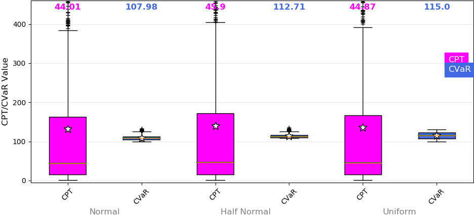
Figure 3: Boxplots showing the distribution of 1000 value samples of CPT and CVaR risk perception model for three different distributions.

VI-B Comparing expressiveness in path planning

Let us suppose that we have an arbitrary example path $P_{d}$ drawn in the environment. If the class of CPT planners is expressive enough, we should be able to find a set of parameters that is able to to exactly mimic this drawn path. Since an arbitrary path $P_{d}$ belongs to a very high dimensional space and the planner parameters are typically finite, any amount of parametric tuning may not produce good approximations. This is what we evaluate in the following. We use the term $\operatorname{Ar}(P;P_{d})\in\mathbb{R}_{\geq 0}$ to denote the area enclosed between the given path $P_{d}$ and another path $P$. This value measures the closeness between $P$ and $P_{d}$.

A path $P$ produced by a CPT planner can be represented by the CPT parameters $\Theta$. In order to find the closest possible path $P^{*}$ to $P_{d}$ we have to evaluate

$$\operatorname*{argmin}_{P_{\Theta},\Theta\in\mathcal{T}}\operatorname{Ar}(P_{\Theta};P_{d}),$$ (7)

where $P_{\Theta}$ is the path produced by CPT-RRT* with CPT parameters $\Theta$, and $\mathcal{T}$ is the set of all possible values of $\Theta$. Directly evaluating (7) is computationally not feasible as the set $\mathcal{T}$ is infinite and resides in $4D$ space.

An alternative to (7) is to use parameter estimation algorithms to determine $\Theta^{*}\in\mathcal{T}$ which characterizes the path $P^{*}$ with $\operatorname{Ar}(P_{\Theta};P_{d})$ as a loss/cost function. We note that neither $\operatorname{Ar}(P_{\Theta};P_{d})$ can be computed directly (without running CPT-RRT* first), nor the gradient of $\operatorname{Ar}$ wrt $\Theta$ is accessible. This limits the use of standard gradient descent algorithms to estimate $\Theta^{*}$. To address this problem, we use SPSA [27] with $\operatorname{Ar}(P_{\Theta};P_{d})$ as the loss function to estimate the parameters $\Theta^{*}$. Next, we briefly explain the main idea and adaptation of SPSA to our setting and refer the reader to [27] for more detailed treatment and analysis of the SPSA algorithm.

We start with an initial estimate $\Theta_{0}$ and iterate to produce estimates $\Theta_{k}$, $k\in\mathbb{Z}_{\geq 0}$ using the loss function measurements $\operatorname{Ar}(P_{\Theta_{k}};P_{d})$. The main idea is to perturb the estimate $\Theta_{k}$ according to  [27] to get $\Theta^{+}$ and $\Theta^{-}$, for the $k^{\textup{th}}$ iteration. These perturbations are then used to generate the perturbed paths $P_{\Theta^{+}},P_{\Theta^{-}}$ using Algorithm 2. With these perturbed paths, the loss function measurements $\operatorname{Ar}(P_{\Theta^{+}};P_{d}),\operatorname{Ar}(P_{\Theta^{-}};P_{d})$ are evaluated and used to update our parameter $\Theta_{k}$ according to [27]. To test the goodness of the updated parameter, we determine the corresponding path $P_{\Theta_{k+1}}$ and measure $\operatorname{Ar}(P_{\Theta_{k+1}};P_{d})$. If the area is within a tolerance $\kappa\in\mathbb{R}_{>0}$, that is, if $\operatorname{Ar}(P_{\Theta_{k+1}};P_{d})<\kappa$, the iteration stops and $P_{\Theta_{k+1}}$ is returned. We followed the guidelines from [27] for choosing the parameters used in SPSA. The results of this adaptation are evaluated and compared with the results that employ other risk perception models in Section VII.

VII Results and Discussion

In this section we illustrate the results of the solutions to the problem statement proposed in Sections IV,V, and VI considering a specific scenario having some risk and uncertainty profiles.

VII-A Environment Perception and Planning

We consider a hypothetical scenario where an agent needs to navigate in a room during a fire emergency. In this, the 2D configuration space for planning becomes $\mathcal{C}=~{}[-10,10]\times[-10,10]$. The agent is shown a rough floor map (Figure 4(a)) with obstacles (which are thought to be ablaze) in the environment with a blot of ink/torn patch, making that region unclear and hard to decipher. This results in the spatial uncertain cost $\rho$ with first moment ($\rho_{\mu}$) represented by cost associated to obstacles and fire source and second moment ($\rho_{\sigma}$) represented by the uncertainty associated to the ink spot/tear.

The blue colored objects are the obstacles whose location is known to be within some tolerance (dark green borders) and the light orange ellipses illustrate that these objects have caught fire. The grey ellipse indicates a possible tear/ink spot on the map, which makes that particular region hard to read. The start and goal positions are indicated as blue spot and green cross respectively. We use a scaled sum of bi-variate Gaussian distribution to model the sources of continuous cost (orange ellipses) with appropriate means and variances to depict the scenario in Figure 4(a). We utilize bump functions from differential geometry to create smooth “bumps” depicting the discrete obstacles. One approach to do this is described in Section III. An alternative procedure is briefly described as follows. Consider the maximum cost value imparted to the obstacles as $\rho^{\textup{max}}\in\mathbb{R}_{\geq 0}$ and let $a_{1},a_{2},b_{1},b_{2}\in\mathbb{R}_{\geq 0}$ be the inner (blue rectangle) and outer (dark green borders) measurements of the obstacles from the center $c=(c_{1},c_{2})\in\mathcal{C}$. Let $x=(x_{1},x_{2})\in\mathcal{C}$ be a point in the configuration space with $f,g,h$ being real valued scalar functions given by $f(y)=e^{-\frac{1}{y}},y\in\mathbb{R}_{>0}\ \text{and}\ f(y)=0\ \text{otherwise}$, $g(y)=\frac{f(y)}{f(y)+f(1-y)}$ and $h(y)=1-g(\frac{y^{2}-a^{2}}{b^{2}-a^{2}})$. Then, $\rho_{\mu}(x)$ can be calculated by :

$$\rho_{\mu}(x)=\rho^{\textup{max}}h(x_{1}-c_{1})h(x_{2}-c_{2}).$$ (8)

This procedure produces smooth “bumps” in the cost profile which are visualized in Figure 4(b) using $\rho^{\textup{max}}=20$. This approach can be easily generalized to arbitrary high dimensions by simply multiplying upto $h(x_{i}-c_{i})$ terms in (8) to create a bump function in the $i^{\textup{th}}$ dimension. To generate the second moment of cost $\rho_{\sigma}$, we use a scaled bi-variate Gaussian distribution with appropriate means and variances to depict the ink spot/tear in Figure 4(a). Now we will illustrate the results of implementing Algorithm 2 in this environment.

Simulations and discussions

With the uncertain cost $\rho$ with moments $\rho_{\mu}$ and $\rho_{\sigma}$ from previous paragraph, we use a half Normal distribution and discretization factor $M=20$ to generate the costs $\rho(x)$ and their corresponding $p(x)$ from Section IV, the results of using Algorithm 1 to every point in $\mathcal{C}$ to generate the perceived environment is shown in Figures 1 and 4. The level of risk at a point $R^{c}$ or $R^{e}$ is indicated by color map. Figure 1(a) shows a rationally perceived environment using expected risk $R^{e}$. Whereas, Figure 1(b) indicates a non-rational highly risk averse perception using CPT ($R^{c}$) with $\Theta=\{0.74,2,0.9,10\}$ having a high $\lambda$ value. A risk indifferent profile (Figure 4(d)) is generated by $\Theta=\{0.74,1,0.3,2.25\}$ having a low risk sensitivity $\gamma$ value. Similarly, uncertainty indifferent profile (Figure 4(e)) and uncertainty averse profile (Figure 4(f)) are generated by fixing $\alpha$ and having high and low $\beta$ values respectively.

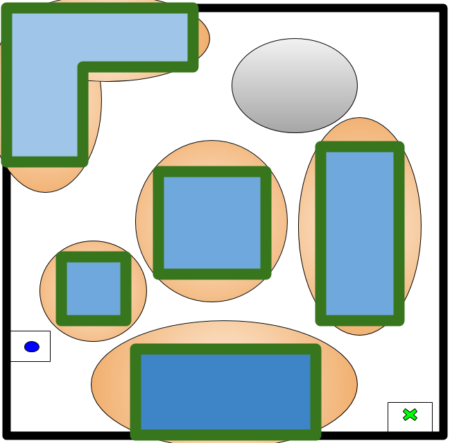
(a) Rough sketch of environment.

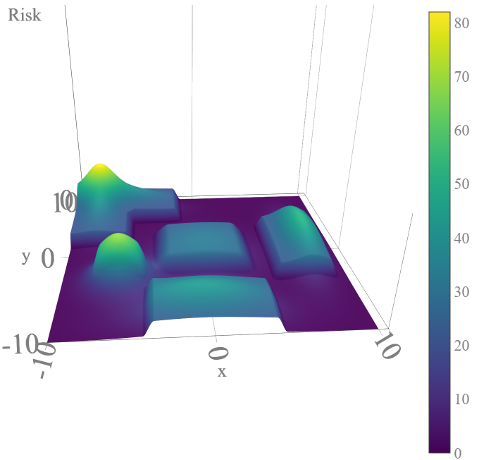
(b) Mean cost $\rho_{\mu}$

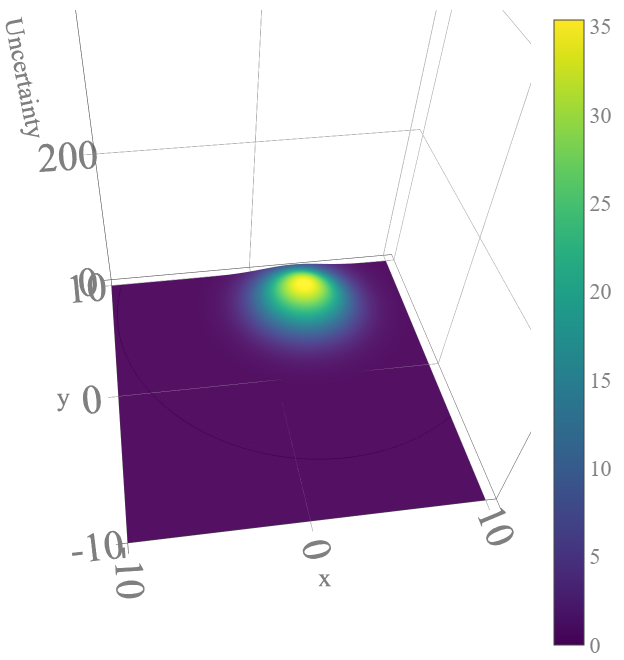
(c) Uncertainty $\rho_{\sigma}$

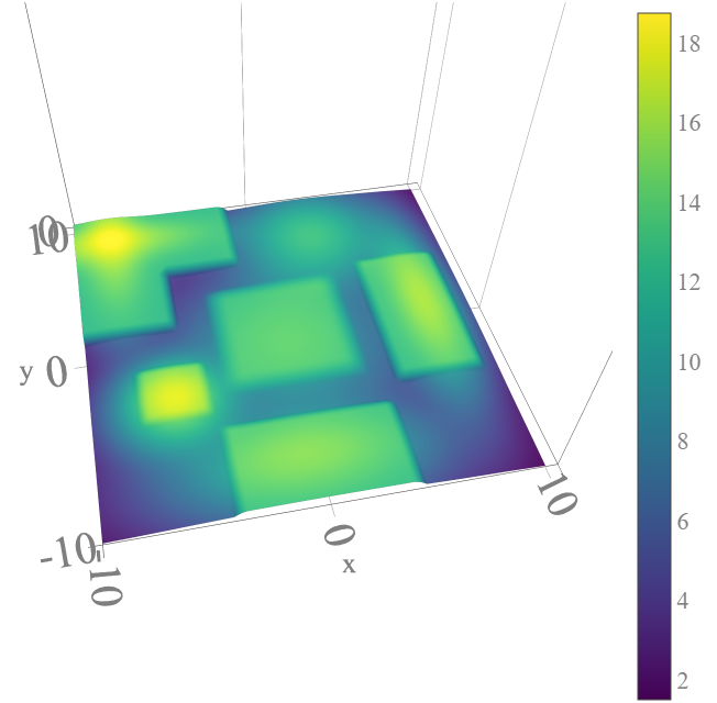
(d) Risk indifferent profile with $\Theta=\{0.74,1,0.3,2.25\}$

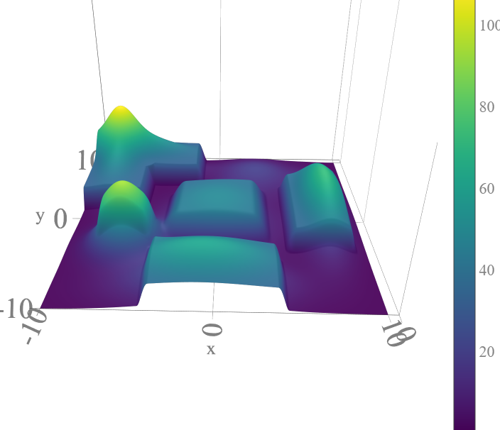
(e) Uncertainty indifferent profile with $\Theta~{}=~{}\{0.74,3,0.88,2.25\}$

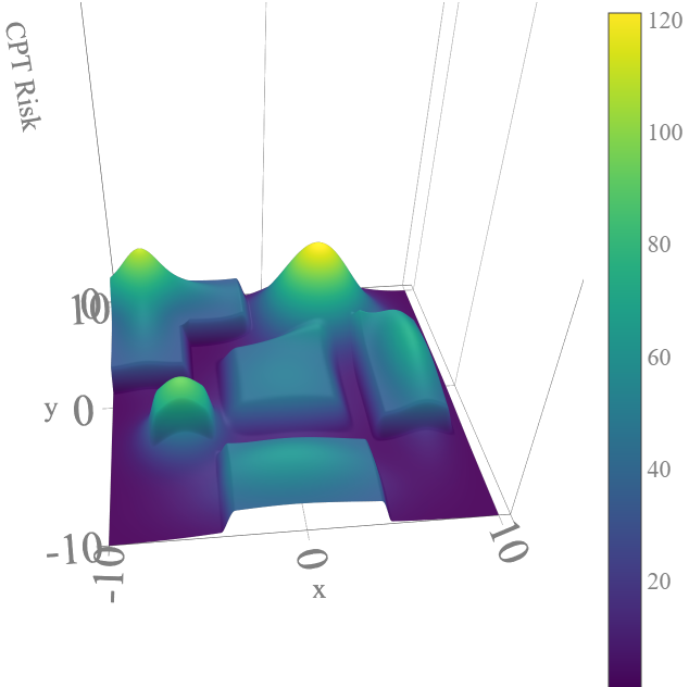
(f) Uncertainty averse profile $\Theta=\{0.74,0.05,0.88,2.25\}$

Figure 4: Environment perception using CPT.

After the perceived environment is generated, Algorithm 2 is used to plan a path from the start point to the goal point shown in Figure 4(a). We use $T=20,000$ iterations for the CPT-RRT* algorithm with $\delta=10^{-4}$. The same random seed was used for all executions for consistency. The path planning results are illustrated in Figure 5. As expected, we see that the path depends on the perceived risk profile. Figure 5(a) indicates a circuitous path due to the highly risk averse perception, whereas Figure 5(d) indicates a shorter and more direct path for a rational DM using expected risk. Increasing the uncertainty sensitivity (lowering $\beta$) and reducing risk aversion (lowering $\lambda$) makes the planner avoid the highly uncertain ink spot/tear in the top-right region and take a more riskier path in the lower region as shown in Figure 5(b). By having a medium risk aversion and lower uncertainty sensitivity (increasing $\beta$), the planner produces a different path through the medium risky and uncertain middle region as shown in Figure 5(c).

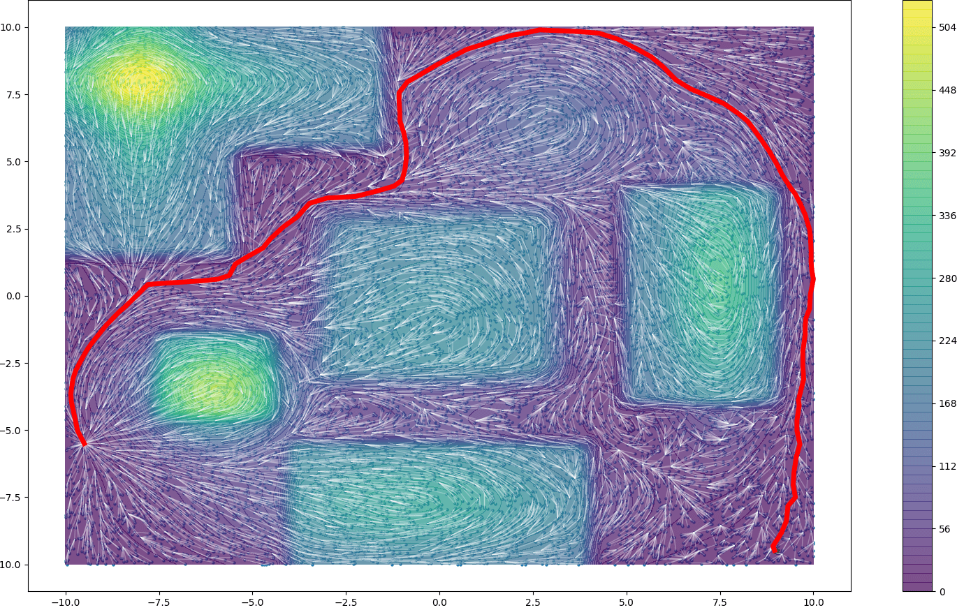
(a) High cost and high uncertainty sensitivity ($\Theta=\{0.74,1,0.9,10\}$)

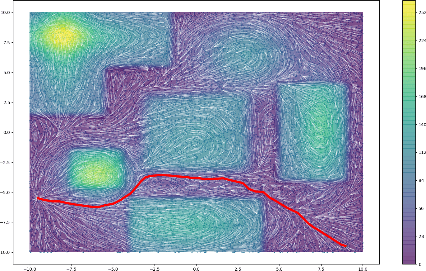
(b) Medium cost aversion and high uncertainty sensitivity ($\Theta=\{0.74,1,0.9,5\}$)

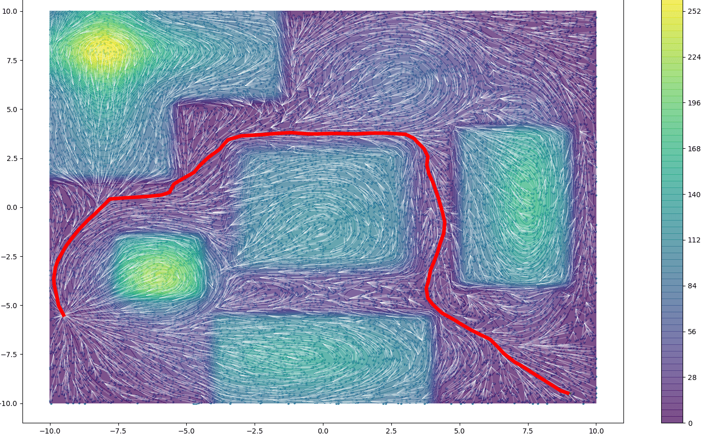
(c) Medium cost aversion and low uncertainty sensitivity ($\Theta=\{0.74,2,0.9,5\}$)

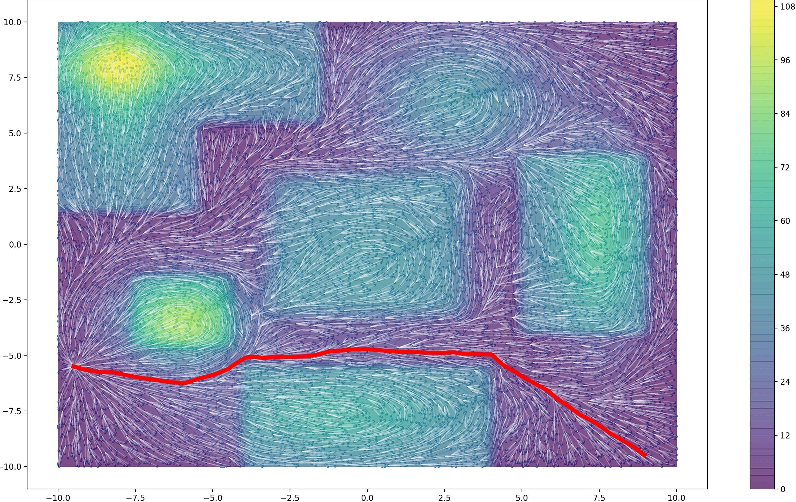
(d) Expected Risk

Figure 5: Paths produced by CPT-RRT* under different perception models. White lines indicate the tree grown from the start position, red line indicates the optimal path to goal after $T=20,000$ iterations. Background color map depicts the CPT costs in (a)-(c) and expected costs in (d)

We also demonstrate the capability of our planner in 3D space, which is illustrated in Fig. 6. We employ a cubic configuration space measuring $10$ units, cluttered with randomly placed $50$ cube obstacles of unit volume. The start position is $(1,1,1)$ and goal position is $(9,9,9)$. There is also a continuous source of risk (modeled as a scaled normal distribution as before) centered at $(3,3,3)$. We use $\Theta=\{0.74,1,0.9,5\}$ (same as 5(b)) with $\gamma_{RRT*}=500$, $d=0.2$ and $\delta=10^{-6}$. From Fig. 6, we see that CPT-RRT is able to find a reasonably smooth path avoiding obstacles and the risky area, in similar number of iterations as in the 2D case. This shows the capability of our planner in 3D space.

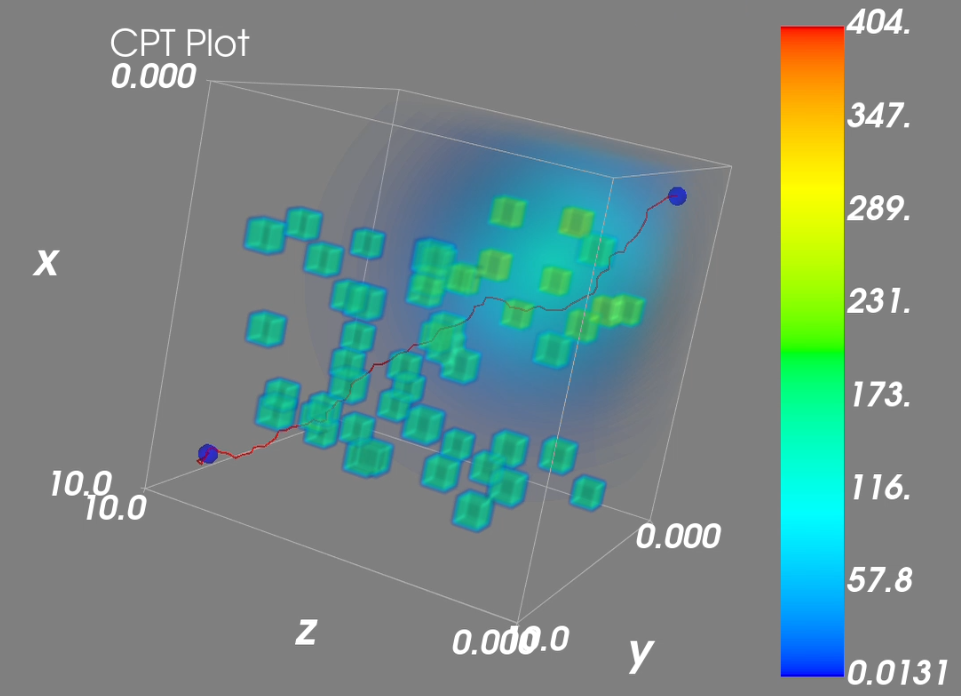
Figure 6: Path(Red line) by CPT-RRT* in 3D environment with 50 discrete random obstacles and a continuous risk source after 20,000 iterations.

Solution quality

Figure 7 illustrates the empirical convergence and solution quality of the paths produced by our algorithm. We performed empirical convergence tests, by running CPT-RRT* $100$ times with the same parameters and initial conditions and measuring the area between paths produced after every $500$ iterations for a total of $80,000$ iterations. The results are shown in Figure 7(a). We see that initially ($<10000$ iterations) there are changes in the output path as the space is being explored and the output path is changing. After $10,000$ iterations we consistently see minimal path changes indicating that the algorithm is converging towards a desirable path. Then we also checked the solution quality of the path by computing the cost of the output path every $250$ iterations as shown in Figure 7(b) for $100$ trials consisting of $25,000$ iteration. We see that the there is a consistent decrease in path cost in all the trials throughout. We also note that after $10,000$ iterations the cost decrease starts to plateau, indicating that the algorithm is close to a high quality (low cost) solution. From these observations of Figure 7, we recommend upwards of $T=10,000$ iterations to achieve smooth and consistent paths in our setting.

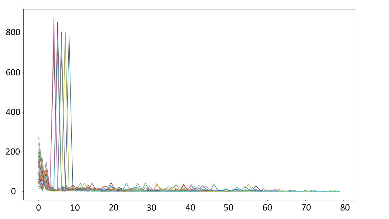
(a) Convergence over iterations

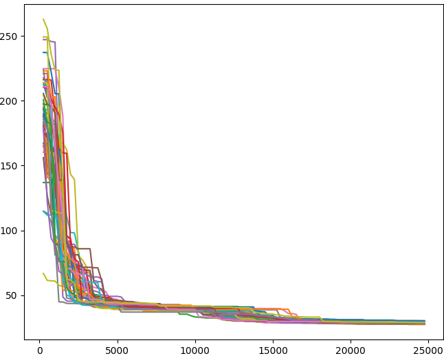
(b) Path cost over iterations

Figure 7: a) Empirical convergence analysis. The distance between paths after every $500$ iterations (y-axis) with the number of iterations in thousand (x-axis). b) Cost of the output path (y-axis) every $250$ iterations with the number of iterations (x-axis)

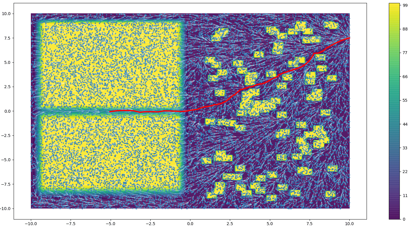
(a) Paths produced by CPT-RRT*.

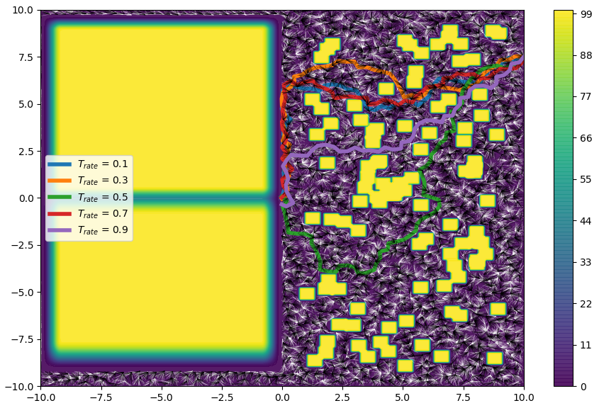
(b) Paths produced by T-RRT* using IC.

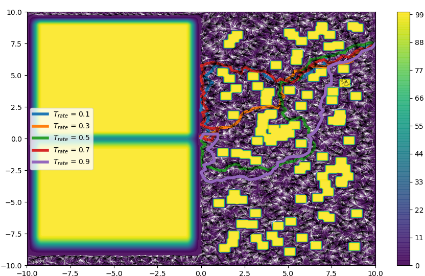
(c) Paths produced by T-RRT* using MW.

(d) Paths produced by varying $\delta$

Figure 8: Path comparison with T-RRT* and varying $\delta$. (a)-(c)Paths produced in a cluttered environment using $T=20,000$ iterations for CPT-RRT* and $20,000$ nodes for T-RRT*. (d) Paths produced by CPT-RRT* by varying $\delta$ with $\Theta=\{0.74,1,0.9,7.5\}$.

Comparison in narrow and cluttered environments

Here, we will illustrate and compare the performance between our RRT* framework and T-RRT* [23] (another algorithm operating on continuous cost spaces) in a cluttered environment with narrow passages as shown in Figure 6. To construct this environment, we used 100 randomly placed small objects on the right half and two big objects separated by a narrow passage on the left half. Start point $x_{s}$ is on the top right corner and the goal $x_{g}$ is at the center of the narrow passage. Bump functions similar to previous paragraphs were used to construct a smooth spatial cost $\rho$ from the obstacles. Since T-RRT* does not have risk perception capabilities, for a fair comparison we use the continuous cost $\rho$ to implement both algorithms. In this way, we will be able to specifically compare the planning capabilities of both algorithms in the same continuous cost environment. We used $\gamma_{\textup{RRT*}}=100$ and $d=0.35$ for both algorithms. From Figure 8(a) we can see that our algorithm is able to sample and generate paths in the narrow passage, as well as avoid obstacles in a cluttered environment. In comparison, we can see that from T-RRT* employing integral cost (IC) in Figure 8(b) and minimum work (MW) in Figure 8(c) cannot generate paths in the narrow costly region fast enough irrespective of the $T_{\textup{Rate}}$ used due to the sampling bias towards low-cost regions. Also, T-RRT* paths do not appear to be as smooth as the paths from our framework, irrespective of the cost(IC or MW) used. We also note that, the cluttered and high cost environment induces a high failure rate of the transition test, resulting in longer run times of T-RRT* required to build the same number of nodes as our algorithm, especially for high $T_{Rate}$ values.

Comparison in dynamic environments

Here, we contrast the performance of CPT-RRT* and Risk-RRT* [20] (a risk aware planner) in a $10$ by $10$ environment area with static and moving obstacles as shown in Figure 9. To account for risk dynamics, we will be planning in the space-time domain, and assume knowledge of the dynamics (or a good estimate) of $\rho_{\mu}(t)$ and $\rho_{\sigma}(t)$, which will result in a time-varying perceived risk map $R^{c}(x,t)$. We also assume that each edge in the tree will be traversed in some time $\Delta t$. The underlying RRT* parameters employed by both algorithms were taken to be identical, with $\gamma_{RRT*}=100$ and $d=0.25$, while $\delta=0.1$ for CPT-RRT*. Our starting point is the same parametric CCR Risk Map [28] as in Risk-RRT*, which generates a continuous, and time-varying, cost map based on the pose and velocity of a moving human as shown in Fig. 9(a) (a snapshot). The human obstacles move back and forth within the indicated range (gray line), with top two obstacles moving $d$ units in $\Delta t$ time, while middle left obstacle moves at $0.1d$ units. Since the CCR map does not incorporate uncertainty, we will use it as the mean cost $\rho_{\mu}(t)$. We employ a scaled normal distribution on top of each source of dynamic risk (moving human) to denote $\rho_{\sigma}(t)$, representing uncertainty for each source. From $\rho_{\mu}(t)$ and $\rho_{\sigma}(t)$, we calculate $R^{c}(x,t)$ according to Algorithm 1 which is visualized in Fig. 9(c). Note that with higher risk (moving obstacles as compared to static or no obstacles), the lighter the color in the map. We compare our algorithm with Risk-RRT* in two scenarios. At first, for fair comparison, and since Risk-RRT* does not consider uncertainty or risk perception models, we use directly the CCR cost map or $\rho_{\mu}(t)$ for planning. This corresponds to a rational DM model. The results are summarized in Fig. 9(b) which show path length and cumulative risk returned by CPT-RRT* and Risk-RRT* using the CCR map in 50 trials. In general, we see a lower performance in Risk-RRT* due to its conservative approach in dealing with risk. First, since risk is not explicitly accounted for in the cost function of Risk-RRT* and “risk” is treated as an “obstacle” to avoid, the resulting path produced by Risk-RRT* is longer, even though its cost function optimizes path length. The length of the path from our planner is shorter, with comparable cumulative risk of the output paths of both planners computed as in (6). Furthermore, $12$ out of the $50$ trials in case of Risk-RRT* could not find a solution within 15,000 iterations. This seems to be a consequence of a higher sample rejection rate due to the tight free spaces created by the dynamic obstacles when close to other objects. This drawback is more pronounced when considering a risk-averse DM. Fig. 9(c) represents such DM who perceives that getting close to the dynamic obstacles is highly risky, as compared to the perception of a rational DM represented by Fig. 9(a). In this way, the risk values in Fig. 9(c) are in the range $0-421$, which is much higher than those of the CCR Map in Fig. 9(a) (with ranges $0-100$). Due to higher risk values as given by this map, the sample rejection in Risk-RRT* is very high and could not find a feasible path in any of $50$ trials, whereas CPT-RRT* consistently found a path similar to the one shown in Fig. 9(c) in all of the 50 trials.

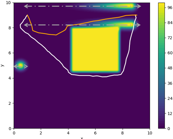
(a) Paths returned by CPT-RRT*(Orange) and Risk-RRT*(White) in CCR map

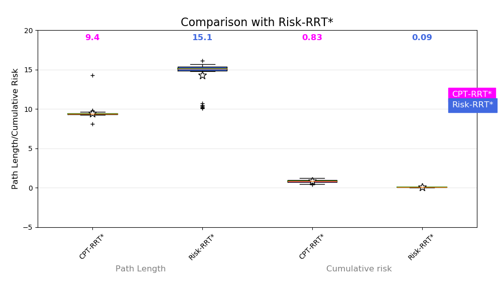
(b) Boxplots showing path length and cumulative risk returned by CPT-RRT* and Risk-RRT* using the CCR map in 50 trials (38 trials for Risk-RRT* as 12 did not succeed in finding a path) consisting of 15,000 RRT* iterations.

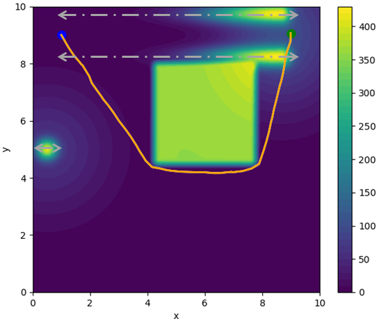
(c) Paths returned by CPT-RRT*(Orange) in risk averse perception of CCR map with $\Theta=\{0.74,1,0.88,6.25\}$

Figure 9: Comparison with Risk-RRT*. The CCR Map containing 3 moving humans and a stationary obstacles at initial time is shown in the background.

Variation in $\delta$

Using the previous environment (Figure 4(a)) and a cost and uncertainty averse profile (Figure 5(a))), we run CPT-RRT* with $\delta$ varying from $\delta=10^{-6}$ to $\delta=10^{2}$ for $T=15,000$ iterations. The results are shown in Figure 8(d). We can see that when $\delta\geq 1$ the path output changes reflecting an increase in urgency over risk and thus choosing shorter paths. When $\delta$ is comparable to the risk values (in this case $\delta=100$), we see that the paths no longer avoid the high risk area and can even go through the soft obstacles. From this study, we observe that $\delta$ needs to be rather small as compared to the given risk profile in order to ensure meaningful consideration of risk in the planning process. If explicit obstacle avoidance is a necessity, then a standard collision check can be performed prior to adding a node in the tree $\mathcal{G}$.

Overall, our adaptation of CPT to the planning setting produces paths that are logically consistent with a given risk scenario. Additionally, our planning framework can explore narrow corridors and cluttered environment and produce smooth paths quickly.

VII-B CPT planner expressive power evaluation

We now discuss the proposed SPSA framework in Section VI to gauge the adaptability of CPT as a perception model to depict a drawn path $P_{d}$. To implement SPSA, we follow guidelines from [27]. We consider a Bernoulli distribution of $\Delta_{k}$ with support $\{-1,1\}$ and equal probabilities, learning rate $a_{k}=\frac{0.4}{(1.6+k)^{0.601}}$ and perturbation parameter $c_{k}=\frac{0.97}{(1.6+k)^{0.301}}$. We choose $\Theta_{0}=\{0.74,1,0.88,2.25\}$ for CPT throughout the simulation, which are the nominal parameters from [4] and $q_{0}=0.5$ for the CVaR variant. We use the same environment as in Figure 4 for all the simulations. Four different paths $\{P^{1}_{d},P^{2}_{d},P^{3}_{d},P^{4}_{d}\}$ are drawn by hand on the expected risk profile (Figure 5(d)) using a computer mouse as shown in Figure 10(a). Path $P^{1}_{d}$ is similar to a path generated with expected risk perception (Figure 5(d)). Whereas, path $P^{4}_{d}$ and $P^{2}_{d}$ are similar to paths generated with high risk aversion (Figure 5(a)) and uncertainty insensitivity (Figure 5(c)) respectively. Path $P^{3}_{d}$ is more challenging to represent as it shows an initial aversion to risk and uncertainty and then takes a seemingly costlier turn at the top. We then use the SPSA approach described in Section VI with a tolerance $\kappa=15$ and a maximum of $10$ SPSA iterations per trial. We use $T_{k}=15000$ iterations and $\delta=0.01$ to implement Algorithm 2 to determine $P_{\Theta}$ in order to determine the loss $\operatorname{Ar}$ during each SPSA iteration. For the CVaR variant, the planner (Algorithm 2) replaces $R^{c}$ with $R^{v}$ in order to use perceived risk according to CVaR while the rest of the RRT* framework remains unchanged. At the end each trial we get the area (loss) $\operatorname{Ar}$ between the returned $P_{\Theta}$ and the drawn path $P^{x}_{d}$.

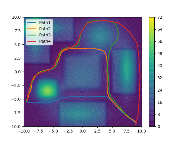
(a) Four paths $\{P^{1}_{d},P^{2}_{d},P^{3}_{d},P^{4}_{d}\}$ are drawn in blue, orange, green and red respectively.

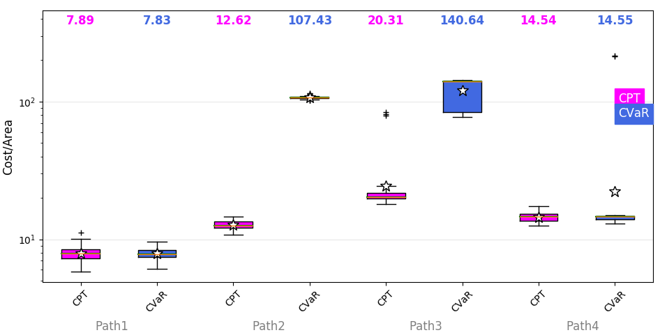
(b) Boxplots showing the cost(Area) returned after using SPSA with CPT and CVaR to capture risk profile of the drawn paths.

Figure 10: Result of using CPT and CVaR to model drawn paths.

We represent the statistics of the returned cost $\operatorname{Ar}$ as boxplots as shown in Figure 10(b). Each box plot represents the distribution of $50$ cost/Area $Ar$ values returned after each trial for each path and perception model. The Y-Axis represents the cost/Area $\operatorname{Ar}$ in a base $10$ log scale. We calculate a few sample areas: $\operatorname{Ar}(P^{1}_{d},P^{2}_{d})=99.14,\operatorname{Ar}(P^{2}_{d},P^{3}_{d})=35.20$ and $\operatorname{Ar}(P^{3}_{d},P^{4}_{d})=73.41$ to give a quantitative idea of the measure $\operatorname{Ar}$ in this scenario to the reader. The median values for each box plot is indicated on the top row. The mean value of the distribution is indicated as “stars”, the black lines above and below the box represent the range, and $+$ indicates outliers. We observe that from Figure 10(b), both Path $P^{1}_{d}$ and Path $P^{4}_{d}$ were captured equally well with CVar and CPT with low $\operatorname{Ar}$ values. Since both CPT and CVaR are generalizations of expected risk, paths close (like $P^{1}_{d}$) to paths generated from expected risk can be easily mimicked. Similarly, since CPT and CVaR are designed to capture risk aversion, paths close (like $P^{4}_{d}$) to risk averse paths (Figure 5(a)) can also be easily captured.

However, we see a contrast in performance for path $P^{2}_{d}$ and path $P^{3}_{d}$. CPT, on both occasions, is able to track the drawn paths reasonably well with low $\operatorname{Ar}$ values. Whereas CVaR has consistently higher (an order of magnitude) $\operatorname{Ar}$ values, indicating the inability to capture the risk perception leading to path $P^{2}_{d}$ and path $P^{3}_{d}$. This is due to the fact that CPT can handle uncertainty perception independently from the cost (as seen between Figure 4(e) and Figure 4(f)). This ability is needed to capture paths like $P^{2}_{d}$ and $P^{3}_{d}$ which is lacking in models like CVaR and expected risk. This shows the generalizability of CPT over CVaR with CPT having a richer modeling capability, thus validating the theoretical results from Lemma 2.

VIII Conclusions and Future Work

We have proposed a novel adaptation of CPT to model a DM’s non-rational perception of a risky environment in the context of path planning. Firstly, using CPT, we provide a tuning knob to model various risk perceptions of an uncertain spatial cost. Next, we demonstrate a novel embedding of non-rational risk perception into a sampling based planner, the CPT-RRT*, to plan asymptotically optimal paths in perceived environments. Finally, we theoretically and empirically evaluate CPT as a good approximator to the risk perception of arbitrary drawn paths by comparing against CVaR, and show that CPT is a richer model approximator. Future work will analyze how CPT can be used to learn the risk profile of a DM using learning frameworks and conducting user studies.

References

- [1] H. Choset, S. Hutchinson, K. M. Lynch, G. Kantor, W. Burgard, L. E. Kavraki, and S. Thrun, Principles of Robot Motion: Theory, Algorithms and Implementations. The MIT Press, 2005.
- [2] C. Wu, A. Bayen, and A. Mehta, “Stabilizing traffic with autonomous vehicles,” in IEEE Int. Conf. on Robotics and Automation, 2018, pp. 1–7.
- [3] A. Suresh and S. Martínez, “Human-swarm interactions for formation control using interpreters,” International Journal of Control, Automation and Systems, 2020, dOI: 1007/s12555-019-0497-3.
- [4] A. Tversky and D. Kahneman, “Advances in prospect theory: Cumulative representation of uncertainty,” Journal of Risk and Uncertainty, vol. 5, no. 4, pp. 297–323, 1992.
- [5] H. Kurniawati, T. Bandyopadhyay, and N. M. Patrikalakis, “Global motion planning under uncertain motion, sensing, and environment map,” Autonomous Robots, vol. 33, no. 3, pp. 1–18, 2012.
- [6] J. Song, S. Gupta, and T. Wettergren, “T*: Time-optimal risk-aware motion planning for curvature-constrained vehicles,” IEEE Robotics and Automation letters, vol. 4, no. 1, pp. 33–40, 2019.
- [7] B. Burns and O. Brock, “Sampling-based motion planning with sensing uncertainty,” in IEEE Int. Conf. on Robotics and Automation, 2007, pp. 3313–3318.
- [8] B. Luders, S. Karaman, and J. How, “Robust sampling-based motion planning with asymptotic optimality guarantees,” in AIAA Conf. on Guidance, Navigation and Control, August 2013.
- [9] L. Blackmore, M. Ono, and B. C. Williams, “Chance-constrained optimal path planning with obstacles,” IEEE Transactions on Robotics, vol. 27, no. 6, pp. 1080–1094, 2011.
- [10] N. E. D. Toit and J. W. Burdick, “Robot motion planning in dynamic, uncertain environments,” IEEE Transactions on Robotics, vol. 28, no. 1, pp. 101–115, 2012.
- [11] S. Singh, Y. Chow, A. Majumdar, and M. Pavone, “A framework for time-consistent, risk-sensitive model predictive control: Theory and algorithms,” IEEE Transactions on Automatic Control, vol. 64, no. 7, pp. 2905–2912, 2019.
- [12] A. Hakobyan, G. Kim, and I. Yang, “Risk-aware motion planning and control using CVaR-constrained optimization,” IEEE Robotics and Automation letters, vol. 4, no. 4, pp. 3924–3931, 2019.
- [13] P. Artzner, F. Delbaen, J. Eber, and D. Heath, “Coherent measures of risk,” Mathematical Finance, vol. 9, no. 3, pp. 203–228, 1999.
- [14] S. Gao, E. Frejinger, and M. Ben-Akiva, “Adaptive route choices in risky traffic networks: A prospect theory approach,” Transportation Research Part C: Emerging Technologies, vol. 18, no. 5, pp. 727–740, 2010.
- [15] A. R. Hota and S. Sundaram, “Game-Theoretic Protection against Networked sis Epidemics by Human Decision-Makers,” IFAC Papers Online, vol. 51, no. 34, pp. 145–150, 2019.
- [16] C. Jie, P. L. A., M. Fu, S. Marcus, and C.Szepesvari, “Stochastic optimization in a Cumulative Prospect Theory framework,” IEEE Transactions on Automatic Control, vol. 63, no. 9, pp. 2867–2882, 2018.
- [17] L. Wang, Q. Liu, and T. Yin, “Decision-making of investment in navigation safety improving schemes with application of Cumulative Prospect Theory,” Journal of Risk and Reliability, vol. 232, no. 6, pp. 710–724, 2018.
- [18] S. Karaman and E. Frazzoli, “Sampling-based algorithms for optimal motion planning,” International Journal of Robotics Research, vol. 30, no. 7, pp. 846–894, 2011.
- [19] B. Boardman, T. Harden, and S. Martínez, “Limited range spatial load balancing in non-convex environments using sampling-based motion planners,” Autonomous Robots, vol. 42, no. 8, pp. 1731–1748, 2018.
- [20] W. Chi and M. Q. Meng, “Risk-RRT*: A robot motion planning algorithm for the human robot coexisting environment,” in Int. Conf. on Advanced Robotics, 2017, pp. 583–588.
- [21] B. Englot, T. Shan, S. D. Bopardikar, and A. Speranzon, “Sampling-based min-max uncertainty path planning,” in IEEE Int. Conf. on Decision and Control, 2016, pp. 6863–6870.
- [22] E. Schmerling, K. Leung, W. Vollprecht, and M. Pavone, “Multimodal Probabilistic Model-based planning for Human-Robot Interaction,” in IEEE Int. Conf. on Robotics and Automation, 2018, pp. 1–9.
- [23] D. Devaurs, T. Simeon, and J. Cortes, “Optimal Path Planning in Complex Cost Spaces with Sampling-based Algorithms,” IEEE Transactions on Automation Sciences and Engineering, vol. 13, no. 2, pp. 415–424, 2016.
- [24] T. Shan and B. Englot, “Sampling-based minimum risk path planning in multiobjective configuration spaces,” in IEEE Int. Conf. on Decision and Control, 2015, pp. 814–821.
- [25] S. Dhami, The Foundations of Behavioral Economic Analysis. Oxford University press, 2016.
- [26] D.Prelec, “The probability weighing function,” Econometrica, vol. 66, no. 3, pp. 497–527, 1998.
- [27] J. C. Spall, Introduction to Stochastic Search and Optimization. New York, 2003.
- [28] W. Chi, H. Kono, Y. Tamura, A. Yamashita, H. Asama, and M. Q. Meng, “A human-friendly robot navigation algorithm using the risk-rrt approach,” in IEEE Int. Conf. on Real-time Computing and Robotics, 2016, pp. 227–232.