Mean field theory of jamming of nonspherical particles

Abstract

Recent computer simulations have uncovered the striking difference between the jamming transition of spherical and non-spherical particles. While systems of spherical particles are isostatic at the jamming point, systems of nonspherical particles are not: the contact number and shear modulus of the former exhibit a square root singularity near jamming, while those of the latter are linearly proportional to the distance from jamming. Furthermore, while our theoretical understanding of jamming of spherical particles is well developed, the same is not true for nonspherical particles. To understand jamming of non-spherical particles, in the previous work [Brito, PNAS 115(46), 111736], we extended the perceptron model, whose SAT/UNSAT transition belongs to the same universality class of jamming of spherical particles, to include additional variables accounting for the rotational degrees of freedom of nonspherical particles. In this paper, we give more detailed investigations of the full scaling behavior of the model near the jamming transition point in both convex and non-convex phases.

• March 2019

1 Introduction

A system consisting of macroscopic particles that are so large that the thermal fluctuations are negligible, at small packing fraction $\varphi$ easily deforms and flows under the action of external driving forces, such as shear and shake. Upon increasing $\varphi$, the constituent particles begin to be in contact and the system has a finite rigidity at a certain critical packing fraction $\varphi=\varphi_{J}$. This non-equilibrium fluid-solid transition is the so-called jamming transition and $\varphi_{J}$ is referred to as the jamming point [1, 2]. The jamming transition has been the focus of an intense research activity, as it is ubiquitously observed in a wide range of engineering and biological systems such as metallic balls [3], foams [4, 5], colloids [6], polymers [7], candies [8], dices [9] and tissues [10].

One of the most popular and simple models to study the jamming transition is a system consisting of frictionless spherical particles with purely repulsive interaction. A large number of numerical works have been performed on this model which have proven that (i) this system is isostatic at $\varphi_{J}$, meaning that the contact number between constituent particles is identical to the number the degrees of freedom, so that the system barely achieves mechanical stability [3], (ii) the distributions of inter particle distances and forces exhibit power law behaviors at $\varphi_{J}$ [11, 12, 13], (iii) various physical quantities, such as the shear modulus and contact number, exhibit power law scaling near $\varphi_{J}$ [5], and (iv) a set of lengthscales diverging at $\varphi_{J}$ [14, 15, 16]. These results suggest that the jamming transition point can be considered as a sort of out-of-equilibrium critical point.

The theoretical understanding of jamming of spherical particles is also quite advanced. On the one hand, M. Wyart et al. developed a variational argument showing that isostaticity plays a crucial role in determining the critical properties of the jamming transition [17, 18]. On the other hand, a system consisting of spherical particles has been solved exactly in the large dimension limit by using the replica liquid theory (RLT) [19, 20]. The RLT is a theory that combines the density functional theory of classical amorphous solids [21, 22, 23] with the replica method [24], which is a standard method to treat disordered systems originally developed to study spin glasses. The RLT predicts that a system near $\varphi_{J}$ is located in the (full) replica symmetric breaking (RSB) phase [25]. In the RSB phase, the system is marginally stable and has a gapless spectrum of excitations [26, 27]. Interestingly, this marginal stability is directly related to the isostaticity of the jamming transition point [28]. The exact solution of hard spheres provides the exact values of the critical exponents of the gap and force distribution function at $\varphi_{J}$ in infinite dimensions, whose values agree well with the numerical results in two and three dimensions within the numerical precision [28, 29, 30, 31].

Furthermore in recent years, Franz and Parisi have proposed to look at the jamming transition point as the satisfiability transition point for continuous constraint satisfaction problems [32]. In a constraint satisfaction problem one has to find a configuration of a set of dynamical variables that satisfy a set of constraints. As the number of constraints increases, one can observe a sharp phase transition from a satisfiable (SAT) phase, where there are configurations of the variables satisfying all the constraints, to an unsatisfiable (UNSAT) phase, where no such configurations exists and a finite fraction of constraints are violated [33, 34, 35]. The jamming transition of spherical particles can be considered as a SAT-UNSAT transition within a glass: in the unjammed phase, one can find disordered configurations satisfying the constraints that spheres do not overlap, meaning that the system is in the SAT phase, while in the jammed phase, one can not find such configurations and the number of contacts between particles is finite, meaning that the system is in the UNSAT phase . In [32] Franz and Parisi considered the simplest continuous constraint satisfaction problem, the perceptron, and showed that the gap and force distributions close to the non-convex SAT/UNSAT (jamming) threshold have the same critical exponents of those of hard spheres in the large dimension limit, implying that the two models belong to the same universality class. The simplicity of the perceptron also allows one to calculate the contact number and the density of states in the jammed (UNSAT) phase, and successfully reproduce the numerical results on jamming of spheres in finite dimensions (even if the origin of this universality is still unclear).

However, spherical particles are an idealized model. In general, asphericity is inevitably introduced in realistic situations (where also friction plays a role, although it will be always neglected here). It has been shown in the last years that the particle shape affects the properties of jamming. Numerical simulations on jamming of ellipsoids shows that the contact number $z_{J}$ at jamming smoothly increases as the asphericity increases, meaning that the system is not isostatic [8, 36]. The breakdown of isostaticity is also observed for spherocylinders [37], superballs [38], superellipsoids [39], other convex shaped particles [40] and even deformable polygons [41]. Furthermore, detailed numerical simulations showed that the critical exponents of the contact number and shear modulus near the jamming transition point differ quite significantly from those of spherical particles [36, 42]. This difference suggests that the universality class of the jamming transition of nonspherical particles is different from the one of spherical objects.

In recent years, a series of phenomenological and theoretical approaches have emerged to rationalize jamming of non-spherical particles. For instance, by analyzing the stability matrix, Donev et al. [43] argue that the breakdown of the isostaticity is caused by the positiveness of the pre-stress term. By using the Edwards ensemble approach, Baule et al. [44] calculated the contact number and the jamming transition point of nonspherical particles, which can qualitatively reproduce the numerical results. However, to the best of our knowledge there is no unified theoretical understanding that explains the origin of the different critical exponents and universality for nonspherical particles. In this work, we study a model that we have recently proposed in a shorter report [45] as a simple exactly solvable mean-field model for the jamming transition of nonspherical particles and we detail its analytical solution. We consider the perceptron model, introduced in [32] to study the jamming transition of spherical particles, and extend it to include additional dynamical variables, playing the same role as the rotational degrees of freedom of nonspherical particles [45]. The model and its scaling properties can be investigated analytically by using the replica method, as in the case of the original perceptron model [46]. We find that the gap and force distributions do not exhibit power law behavior and remain regular even at the jamming transition point. This is in marked constrast with the original perceptron model or spherical particles, where the gap and force distributions exhibit power laws [46]. We find that the absence of criticality of the gap and force distributions are originated from the breakdown of isostaticity at the jamming transition point, as predicted in [17, 18]. Furthermore, the regularity of these distributions leads to a trivial linear distance dependence of the physical quantities near the jamming transition point. We find that the critical exponents change discontinuously at zero asphericity, meaning that an infinitesimal asphericity is enough to alter the universality of the jamming transition.

The paper is organized as follows. In Sec. 2, we introduce the model and in Sec. 3, we derive the free energy and saddle point equations with the replica method. In Sec. 4, we calculate the phase diagram using the replica symmetric ansatz. In Sec. 5, we argue the scaling behavior of the model above and at the jamming transition point and in Sec. 6, we calculate the density of states in the UNSAT(jammed) phase and compare it with previous numerical results on ellipsoids. Finally in Sec. 7, we summarize our results and give some perspectives. We discuss the technical details in the appendix.

2 The polydisperse perceptron model

Jamming of particles can be regarded as a special case of a more general class of problems where one needs to find an assignement of a large set of continuous variables to satisfy a set of constraints [32]. These problems are therefore called Continuous Constraint Satisfaction Problems (CCSP). In this general setting, there is a precise dictionary between jamming of spheres and CCSP that allows to identify several physical quantities, from the pressure to gap variables and number of contacts, in both class of problems. Here we will not review this dictionary extensively but we will limit ourselves to discuss it online while presenting the application of this line of reasoning to study jamming of non-spherical particles. The interested reader can find more details in [26, 46].

The perceptron is a well known and studied linear classifier in machine learning [47, 48, 49, 50]. Here, following [32], we turn it into a continuous constraint satisfaction/optimization problem to study the jamming transition. The model studied in [32] is defined in terms of a state vector $\bm{x}=\{x_{1},\ldots,x_{N}\}$ which is $N$-dimensional and lives on the $(N-1)$-dimensional hypersphere defined by $|\bm{x}|^{2}=N$. Furthermore one defines a set of $M=\alpha N$ quenched $N$-dimensional random vectors $\{\bm{\xi}^{\mu}=\{\xi^{\mu}_{1},\ldots,\xi^{\mu}_{N}\}\}_{\mu=1,\ldots,M}$ whose components are Gaussian random variables with zero mean and unit variance. Given each random vector (often referred to as “pattern”) and the state vector of the system, one can define a gap variable as

$$h_{\mu}=\frac{\bm{x}\cdot\bm{\xi}^{\mu}}{\sqrt{N}}-\sigma.$$ (1)

where $\sigma$ is a control parameter. The constraint satisfaction problem is defined by asking for a vector $\bm{x}$ that satisfies all the constraints

$$h_{\mu}\geq 0\ \ \ \ \ \forall\mu=1,\ldots,M\>.$$ (2)

On general grounds one can expect that if $\alpha$ is small enough it is possible to find a satisfiable (SAT) configuration of $\bm{x}$ while if $\alpha$ is large enough this is not possible and the problem becomes unsatisfiable (UNSAT). Indeed, in the thermodynamic limit $N\to\infty$, there exists a sharp SAT/UNSAT phase transition that marks the boundary between the two phases. The parameter $\sigma$ controls the convexity of the problem: if $\sigma>0$ the constraint satisfaction problem is convex while if $\sigma<0$ it is non-convex. In [32] it has been shown that for $\sigma<0$ the problem has a replica symmetry breaking phase near the jamming point as hard spheres in infinite dimensions [25], and the SAT/UNSAT transition is in the same universality class of jamming of spherical particles.

In this work, the perceptron model is extended to describe the jamming of nonspherical particles. We consider the polydisperse perceptron model that has been introduced in [45] and here we first recall its definition and then we construct its full analytical solution. For non-spherical particles like ellipsoids, the relative distance between constituent particles depends on their relative angles. Therefore the actual gap between particles is a function of both the distance of their centers and relative orientation. More precisely, consider non-spherical particles, with $\Delta$ being the linear deviation from spherical shape (for example, in ellipsoids $\Delta$ is the deviation of the aspect ratio from 1) and with the asphericity parameter being

$$\mathcal{A}(\Delta)=\frac{S_{d}(\Delta)}{V_{d}(\Delta)^{\frac{d-1}{d}}}\frac{V_{d}(0)^{\frac{d-1}{d}}}{S_{d}(0)}-1\ ,$$ (3)

where $S_{d}(\Delta)$ and $V_{d}(\Delta)$ represent the surface and volume of a $d$-dimensional particle, respectively. Note that because the function $\mathcal{A}(\Delta)$ has a minimum at $\Delta=0$, it can be expanded as $\mathcal{A}(\Delta)=\mathcal{A}^{\prime\prime}(0)\Delta^{2}/2+\cdots$, which leads to $\Delta\sim\mathcal{A}^{1/2}$. Note also that for small $\Delta$, the gap between two particles can be written as [45]

$$h(r,\theta)\sim h(r)+\Delta\,f(\theta)\ ,$$ (4)

where $r$ is the distance between the centers, $h(r)=r-\sigma$ is the gap for spherical particles of diameter $\sigma$, and $f(\theta)$ is some function of the non-spherical degrees of freedom.

One can think about the orientation of a particle as a dynamical internal degree of freedom that each particle can change in order to satisfy better the constraints. In this way one can construct more general models in which beyond the standard degrees of freedom that are the position of the particles, one can consider internal degrees of freedom that must have the same role as orientations for non-spherical particles. In practice, any internal degree of freedom such that Eq. (4) holds should lead to similar results. For example, in [45] we have shown that in the small asphericity limit, the interaction potential of ellipsoids maps to the interaction potential of a model of breathing spheres, namely spheres that can change their diameter [51]. This suggests that one can extend the perceptron model studied in Ref. [32, 46], by replacing the effective diameter $\sigma$ by a fluctuating one [45]

$$\sigma\to\sigma+\Delta R_{\mu}\ ,$$ (5)

so that the new gap variables become

$$h_{\mu}=\frac{\bm{x}\cdot\bm{\xi}^{\mu}}{\sqrt{N}}-\sigma-\Delta R_{\mu}\>.$$ (6)

The variables $\{R_{\mu}\}_{\mu=1,\ldots M}$ are additional internal dynamical variables that can be used to find solutions to the constraint satisfaction problem. We bound their amplitude by enforcing them to live on a $(M-1)$-dimensional hypersphere

$$|\bm{R}|^{2}\equiv\sum_{\mu=1}^{M}R_{\mu}^{2}=M\>.$$ (7)

Because Eq. (6) has the same structure of Eq. (4), we expect this modified perceptron to fall into the same universality class of non-spherical particles with $\mathcal{A}\sim\Delta^{1/2}$. The control parameter $\Delta$ thus tunes the asphericity of the problem: in the limit $\Delta\to 0$, the model reduces to the standard perceptron model, which corresponds to the system consisting of spherical particles, except at the jamming transition point. However at the jamming transition point, the model leads to the completely different scaling from the standard perceptron even in the $\Delta\to 0$ limit, as we discuss in the rest of the manuscript.

In order to solve the constraint satisfaction problem defined by the polydisperse perceptron model we can define a cost function

$$U_{N} =\sum_{\mu=1}^{M}v(h_{\mu})\ .$$ (8)

The local potential $v(h_{\mu})$ has to satisfy the property that

$$v(h)\begin{cases}=0&h\geq 0\\ >0&h<0\>.\end{cases}$$ (9)

The choice that we adopt here is the one describing harmonic particles $v(h)=h^{2}\theta(-h)/2$. The particular choice of the cost function does not affect the SAT phase as well as the SAT/UNSAT threshold, while it deeply affects the properties of the jammed phase [46, 52]. In order to impose the spherical constraint of Eq. (7) we add a chemical potential $\mu_{N}$ to the cost $U_{N}$ so that the final interaction potential reads

$$V_{N}=U_{N}+\mu_{N},\qquad U_{N}=\sum_{\mu=1}^{M}v(h_{\mu}),\qquad\mu_{N}=\frac{k_{R}}{2}\sum_{\mu=1}^{M}R_{\mu}^{2}$$ (10)

where $k_{R}$ is a Lagrange parameter used to enforce Eq. (7). In the next section we study the partition function of the model at inverse temperature $\beta=1/T$ defined as

$$Z=\int_{|\bm{x}|^{2}=N}\mathrm{d}\bm{x}\int_{|\bm{R}|^{2}=M}\mathrm{d}\bm{R}\,e^{-\beta V_{N}}$$ (11)

and we study the corresponding average free energy using the replica method [24].

3 Free energy and thermodynamic quantities

The free energy of the model can be calculated by using the replica trick:

$$-\beta f=\lim_{n\to 0}\frac{\log\overline{Z^{n}}}{nN},$$ (12)

where the overline denotes the average over the disorder $\{\bm{\xi}^{\mu}\}_{\mu=1,\ldots,M}$. As usual for integer $n$, one interprets the $n$th power of the partition function as the partition function of a system of $n$ copies or replicas of the original system, all subjected to the same realization of disorder. In this way, using standard manipulations, the free energy of the replicated system can be obtained as

$$-\beta nf\equiv\frac{\log\overline{Z^{n}}}{N}\approx\frac{1}{2}\log\det Q-n\frac{\alpha}{2}\log\tilde{k}+\alpha\log\left(e^{\frac{1}{2}\sum_{ab}Q_{ab}\frac{\partial^{2}}{\partial h_{a}\partial h_{b}}}\left.\prod_{a=1}^{n}e^{-\beta\phi_{\rm eff}(h_{a})}\right|_{h_{a}=0}\right),$$ (13)

where $\tilde{k}=\beta k_{R}$, and $Q$ denotes the $n\times n$ overlap matrix $Q_{ab}=\left\langle\bm{x}^{a}\cdot\bm{x}^{b}\right\rangle/N$, $a,b=1,\cdots,n$ that has diagonal elements equal to one due to the spherical constraint on $\bm{x}$ while its off diagonal elements are obtained as a saddle point of Eq. (13). In Eq. (13) we have also introduced the effective potential

$$e^{-\beta\phi_{\rm eff}(r)}=\gamma_{\Delta^{2}/\tilde{k}}*e^{-\beta v(r)}.$$ (14)

Here $\gamma_{A}(x)$ denotes a Gaussian function of zero mean and variance $A$, and the star product denotes the convolution, $f*g(x)=\int_{-\infty}^{\infty}\mathrm{d}yf(y)g(x-y)$. The parameter $k_{R}$ should also be determined by a saddle point of Eq. (13), in order to enforce the constraint in Eq. (7). The saddle point equations for the overlap matrix $Q$ can be solved only assuming some ansatz that allows one to take the analytic continuation $n\to 0$. Following the standard strategy of replica theory, we assume a hierarchical ansatz for $Q$ [53], in which $Q$ is encoded by a continuous function $q(x)$ defined for $x\in[0,1]$ with the boundary conditions $q(x)=q_{m}$ for $x\in[0,x_{m})$ and $q(x)=q_{M}$ for $x\in(x_{M},1]$. It is practical to define $x(q)$ as the inverse function of $q(x)$ for $x\in[x_{m},x_{M}]$. After a standard but slightly lengthy procedure (see A and [46]), one obtains the saddle point condition for $x(q)$ as the solution of:

$$\frac{q_{m}}{\lambda(q_{m})^{2}}+\int_{q_{m}}^{q}\mathrm{d}p\frac{1}{\lambda(p)^{2}} =\alpha\int\mathrm{d}hP(q,h)f^{\prime}(q,h)^{2}\ ,$$ (15)

where

$$\lambda(q) =1-q_{M}+\int_{q}^{q_{M}}\mathrm{d}px(p)\ .$$ (16)

In Eq. (15), $f(q,h)$ and $P(q,h)$ are the solutions of the Parisi equations

$$\dot{f}(q,h) =-\frac{1}{2}\left[f^{\prime\prime}(q,h)+x(q)f^{\prime}(q,h)^{2}\right],$$

$$\dot{P}(q,h) =\frac{1}{2}\left[P^{\prime\prime}(q,h)-2x(q)\left(P(q,h)f^{\prime}(q,h)\right)^{\prime}\right],$$ (17)

where $\dot{g}(q,h)=\partial g(q,h)/\partial q$ and $g^{\prime}(q,h)=\partial g(q,h)/\partial h$, and the boundary conditions are

$$f(q_{M},h) =\log\gamma_{1-q_{M}+\Delta^{2}/\tilde{k}}*e^{-\beta v(h)}\ ,$$

$$P(q_{m},h) =\gamma_{q_{m}}(h+\sigma)\ .$$ (18)

In the continuous RSB phase, $x(q)$ becomes a monotonic function of $q$, suggesting that Eq. (15) can be differentiated w.r.t. $q$ [46, 54]. The first and second derivatives lead to

$$\frac{1}{\lambda(q)^{2}} =\alpha\int\mathrm{d}hP(q,h)f^{\prime\prime}(q,h)^{2},$$ (19)

$$x(q) =\frac{\lambda(q)}{2}\frac{\int\mathrm{d}hP(q,h)f^{\prime\prime\prime}(q,h)^{2}}{\int\mathrm{d}hP(q,h)\left[f^{\prime\prime}(q,h)^{2}+\lambda(q)f^{\prime\prime}(q,h)^{3}\right]}.$$ (20)

Finally, the spherical constraint for $R_{\mu}$, Eq. (7), reduces to

$$1 =\frac{1}{\tilde{k}}+\frac{\Delta^{2}}{\tilde{k}^{2}}\int\mathrm{d}hP(q_{M},h)\left[f^{\prime\prime}(q_{M},h)+(f^{\prime}(q_{M},h))^{2}\right].$$ (21)

Eqs. (15-21) represent the set of saddle point equations through which we can obtain the free energy of the model.

For later convenience, we introduce several thermodynamic quantities that we shall discuss in this manuscript. First we define the gap distribution as the following Boltzmann average

$$\rho(h)=\frac{1}{M}\left\langle\sum_{\mu=1}^{M}\delta(h-h_{\mu})\right\rangle,$$ (22)

which can be calculated from the first derivative of the free energy w.r.t. the interaction potential [46]:

$$\rho(h)=\frac{1}{\alpha}\frac{\delta f}{\delta v(h)}=e^{-\beta v(h)}\int\mathrm{d}zP(q_{M},z)e^{-f(q_{M},z)}\gamma_{1-q_{M}+\Delta^{2}/k_{R}}(z-h)\ .$$ (23)

Using $\rho(h)$, one can calculate the isostaticity index as

$$z \equiv\frac{1}{N}\left\langle\sum_{\mu=1}^{M}\theta(-h_{\mu})\right\rangle=\alpha\int\mathrm{d}h\rho(h)\theta(-h).$$ (24)

The value of $z$ equals one when the system is isostatic, namely, when the number of UNSAT gaps is equal to the dimension of $\bm{x}$. Note that the normalization of Eq. (24) is $N$, which is not the total number of degrees of freedom given by $N+M$ . The pressure $p$ is also calculated from $\rho(h)$:

$$p \equiv-\frac{1}{N}\left\langle\sum_{\mu=1}^{M}h_{\mu}\theta(-h_{\mu})\right\rangle=-\alpha\int\mathrm{d}h\rho(h)h\theta(-h).$$ (25)

For comparison with numerical results, we introduce the positive gap distribution

$$g(h) \equiv\theta(h)\frac{\rho(h)}{\int_{0}^{\infty}\mathrm{d}h\rho(h)},$$ (26)

and the force distribution

$$P(f) \equiv\theta(-h)\frac{\rho(h)\frac{dh}{df}}{\int_{-\infty}^{0}\rho(h)\frac{dh}{df}\mathrm{d}f},$$ (27)

where $f=-h/p$ for negative $h$.

4 Phase diagram

4.1 Replica symmetric jamming transition point

We first consider the simplest ansatz for $Q$, namely the replica symmetric (RS) form $Q_{ab}=\delta_{ab}+(1-\delta_{ab})q$. In this case the corresponding saddle point equations reduce to

$$\frac{q}{(1-q)^{2}}=\alpha\int\mathrm{d}hP_{\rm RS}(q,h)f_{\rm RS}^{\prime}(q,h)^{2}\ ,$$ (28)

where

$$f_{\rm RS}(q,h) =\log\gamma_{1-q+\Delta^{2}/\tilde{k}}*e^{-\beta v(h)},$$

$$P_{\rm RS}(q,h) =\gamma_{q}(h+\sigma)\>.$$ (29)

We want to consider what happens in the zero temperature limit where the partition function gives either the Gardner volume of solutions of the constraint satisfaction problem [48, 55] in the SAT phase or the ground state energy in the UNSAT phase. In this second case the overlap $q$ parametrizes the typical overlap between two configurations in the ground state basin and therefore for $T\to 0$ we have that $q\to 1$. Therefore we can expand $q$ as [46]

$$q\approx 1-T\chi,$$ (30)

where $\chi$ is a constant. At the jamming transition point, $\chi$ diverges to infinity since in the SAT phase $q<1$ [46]. For $\beta\gg 1$, we obtain (see Appendix C in Ref. [46])

$$f_{\rm RS}(q,h)\sim-\beta\frac{h^{2}}{2(1+\chi+\Delta^{2}/k_{R})}\theta(-h).$$ (31)

Substituting this into Eq. (28), we obtain

$$\left(1+\frac{1}{\chi}+\frac{\Delta^{2}}{k_{R}\chi}\right)^{2}=\alpha G(\sigma),$$ (32)

where we have introduced an auxiliary function:

$$G(\sigma)=\int_{-\infty}^{0}dh\gamma_{1}(h+\sigma)h^{2}.$$ (33)

With a similar calculation, one can show that Eq. (21) reduces to

$$1=\frac{\Delta^{2}}{(\Delta^{2}+k_{R}(1+\chi))^{2}}G(\sigma).$$ (34)

Eqs. (32) and (34) can be solved for $k_{R}$,

$$k_{R}=\frac{\Delta}{\chi\sqrt{\alpha}},$$ (35)

which implies that $k_{R}$ vanishes on approaching the jamming transition point as $k_{R}\sim\chi^{-1}$. Substituting this into Eq. (32) and taking the $\chi\to\infty$ limit, we obtain the jamming transition point $\alpha_{J}$:

$$\alpha_{J}(\sigma,\Delta) =\left(\frac{1}{\sqrt{G(\sigma)}-\Delta}\right)^{2}.$$ (36)

The same equation is obtained by investigating the saddle point equations in the unjammed phase, see B. In Fig. 1, we show the typical behavior of $\alpha_{J}$ calculated by Eq. (36) for $\Delta=0.1$.

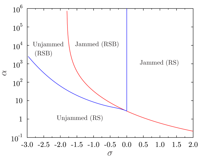
Figure 1: Phase diagram of the perceptron for $\Delta=0.1$. The red line denotes the jamming transition point computed using a replica symmetric ansatz. The blue lines denote the RS-RSB transition. Picture taken from Ref. [45].

$\alpha_{J}$ increases with decreasing $\sigma$, which is a reasonable result considering that $\sigma$ corresponds to the effective diameter. For fixed $\sigma$, $\alpha_{J}$ increases as $\Delta$ increases, which is consistent with the numerical results of nonspherical particles of small asphericity [37, 8, 38, 40]. On the contrary, for larger asphericity, the jamming density of a particle system exhibits a non-monotonic behavior [37, 8, 38, 40], which is not captured by this extended perceptron model, which only represents nonspherical particles with small asphericity up to $O(\Delta^{2})=O(\mathcal{A})$ [45].

4.2 RS-RSB phase boundary

The RS ansatz breaks down in the (full) replica symmetric breaking (RSB) phase where $q(x)$ becomes a continuous function of $x$. In this case, the inverse function $x(q)$ is also a continuous function of $q$. Thus, at the RS-RSB phase boundary, $q$ calculated with the RS ansatz should satisfy Eq. (19), which leads to

$$\left(1+\frac{1}{\chi}+\frac{\Delta^{2}}{k_{R}\chi}\right)^{2}=\alpha\int_{-\infty}^{0}dh\gamma_{1}(h+\sigma).$$ (37)

Using Eqs. (32) and (37), it can be shown that the RS-RSB boundary in the jammed phase is the vertical line defined by $\sigma=0$, see the blue vertical line in Fig. 1. Similarly, one can calculate the RS-RSB phase boundary by substituting the RS result in the unjammed phase into Eq. (19), see the blue line in the unjammed phase of Fig. 1. The resulting figure shows that the jamming transition line lies in the RSB region when $\sigma<0$, as in the case of the standard spherical perceptron [32].

5 Jamming scaling in the RSB phase

In this section, we discuss the scaling behavior of the jamming transition for $\sigma<0$, where jamming is described by the RSB equations and belongs to the same universality class of particle systems. For the sake of brevity, here we only discuss the scaling in the jammed phase, but the scaling solutions in the unjammed phase can be constructed in a very similar way, see C for the details.

5.1 Scaling solutions in the zero temperature limit

First we derive the asymptotic forms of the relevant equations in the zero temperature limit, $T\to 0$. As in the case of the RS analysis, we expand as $q_{M}=1-T\chi$, where $\chi$ has a finite limit for $T\to 0$ and diverges at the jamming transition point. We introduce the following scaling variables for $\chi\gg 1$ [46]:

$$K =\frac{\chi k_{R}}{\Delta^{2}}, y(q) =\frac{\beta}{\chi}x(q), \pi(q) =1+\frac{1}{K}+\int_{q}^{1}dpy(p), m(q,h) =\pi(q)f^{\prime}(q,h)\ .$$ (38)

Then, the gap distribution $\rho(h)$, Eq. (23), is

$$\rho(h)\sim\theta(h)P(1,h)+\theta(-h)(1+\chi+\Delta^{2}/k_{R})P(1,(1+\chi+\Delta^{2}/k_{R})h).$$ (39)

Using Eq. (24) and (19), we obtain

$$z =\left(1+\frac{1}{\chi}+\frac{1}{K}\right)^{2}.$$ (40)

Away from the jamming point, it has been shown that $y(q)$ is described by the following scaling solution near $q\sim 1$ [46]:

$$y(q) \sim\frac{\mathcal{Y}}{\sqrt{1-q}},$$ (41)

which we refer to as the “regular” solution. For $m(q,h)$, we assume

$$m(q,h) \sim-\frac{\chi(1+K^{-1})}{1+\chi(1+K^{-1})}\sqrt{1-q}\mathcal{M}\left(\frac{h}{\sqrt{1-q}}\right).$$ (42)

Using Eq. (20), one can calculate $\mathcal{Y}$ as

$$\mathcal{Y} \sim\frac{K+\chi K+\chi}{2(K+\chi)}\frac{P(1,0)\int dt\mathcal{M}^{\prime\prime}(t)^{2}}{\int_{-\infty}^{0}dhP(1,h)}.$$ (43)

5.2 Jamming for $\Delta=0$

For self-completeness, we first review the scaling behavior of the standard perceptron model ($\Delta=0$), which corresponds to the jamming of spherical particles and has been already well investigated in previous work [46]. In this case, the isostaticity index defined in Eq. (40) reduces to [46]

$$z =\left(1+\frac{1}{\chi}\right)^{2}.$$ (44)

At the jamming transition point, $\chi\to\infty$, one obtains

$$z\to 1,$$ (45)

meaning that the system becomes isostatic: the number of contacts is the same of that of the degree of freedom. Away from the jamming transition point, $z$ increases as

$$\delta z \equiv z-1=\frac{1}{\chi}.$$ (46)

For $\Delta=0$, Eq. (43) reduces to

$$\mathcal{Y} \sim\frac{1+\chi}{2}\frac{P(1,0)\int dt\mathcal{M}^{\prime\prime}(t)^{2}}{\int_{-\infty}^{0}dhP(1,h)}$$ (47)

and for $\chi\gg 1$, we get

$$\mathcal{Y} \sim\chi P(1,0)\sim\delta z^{-1}P(1,0),$$ (48)

implying that the scaling solution Eq. (41) breaks down when the system becomes isostatic and $\delta z=0$. Indeed in the isostatic limit, the scaling ansatz for $y(q)$ becomes:

$$y(q)\sim\frac{y_{J}}{(1-q)^{1/\kappa}},$$ (49)

where the value of the critical exponent $\kappa=1.41574\ldots$ is obtained by solving the Parisi equations in the scaling regime [46]. Hereafter, we shall refer to Eq. (49) as the “critical” scaling solution. The matching argument between the regular and critical scaling solutions determines the asymptotic behavior of $P(1,h)$ as [46]

$$P(1,h)\sim\begin{cases}\chi p_{-}(h\chi)&{\rm for}\ h\sim-\chi^{-1},\\ \chi^{\gamma\psi}p_{0}(h\chi^{\psi})&{\rm for}\ \left|h\right|\sim\chi^{-\psi},\\ p_{+}(h)&{\rm for}\ h\gg\chi^{-\psi},\end{cases}$$ (50)

where

$$p_{+}(t\to 0^{+}) \sim t^{-\gamma}, p_{0}(t\to\infty) \sim t^{-\gamma}, p_{-}(t\to 0^{-}) \sim\left|t\right|^{\theta}, p_{0}(t\to-\infty) \sim\left|t\right|^{\theta}.$$ (51)

The critical exponents are

$$\gamma =\frac{2-\kappa}{\kappa}=0.413, \theta =\frac{3\kappa-4}{2-\kappa}=0.421, \psi =\frac{\kappa}{2(\kappa-1)}=1.703.$$ (52)

Using Eqs. (25), (39) and (50), the pressure is calculated as

$$p =-\alpha\int_{-\infty}^{0}dhP(1,h)h\sim-\delta z^{2}\int_{-\infty}^{0}dtp_{-}(t)t,$$ (53)

leading to

$$\delta z\sim p^{1/2}.$$ (54)

This is consistent with the numerical results of the jamming transition of spherical particles interacting with the harmonic potential [5]. Using Eqs. (26), (27), (39), and (50), we arrive at the asymptotic forms of the positive gap and force distributions:

$$g(h) \sim\begin{cases}\delta z^{-\psi\gamma}p_{0}(h\delta z^{-\psi})&(h\sim\delta z^{\psi}),\\ h^{-\gamma}&(h\sim 1)\end{cases},$$

$$P(f) \sim\begin{cases}\delta z^{\theta\omega}p_{0}(f\delta z^{-\omega})&(f\sim\delta z^{\omega})\\ f^{\theta}&(f\sim 1)\end{cases},$$ (55)

where

$$\omega =\psi-1=0.703.$$ (56)

Eqs. (55) show that the gap and force distributions exhibit a power law behavior if the system is isostatic, $\delta z=0$, while they remain finite and regular if the system is not isostatic, $\delta z\neq 0$.

5.3 Jamming for $\Delta>0$

We now discuss the scaling behavior for $\Delta>0$, corresponding to the jamming of nonspherical particles. We first study the equations in the jamming limit, $\chi\to\infty$. The isostaticity index at the jamming transition point is

$$z=\left(1+\frac{1}{K}\right)^{2},$$ (57)

implying that

$$\delta z\sim\frac{1}{K}\neq 0.$$ (58)

Eq. (43) at the jamming point becomes

$$\mathcal{Y} \sim\frac{1+K}{2}\frac{P(1,0)\int dt\mathcal{M}^{\prime\prime}(t)^{2}}{\int_{-\infty}^{0}dhP(1,h)}.$$ (59)

Note that, unlike for jamming of spherical particles, $\mathcal{Y}\sim KP(1,0)\sim\delta z^{-1}P(1,0)$ remains finite even at jamming, implying that the regular scaling solution, described by Eq. (41) persists even at the jamming transition. The regular solution connects to the critical solution described by Eq. (49), in the spherical limit $\Delta\to 0$. It is worth noting that Eqs. (44) and (47) can be identified with Eqs. (57) and (59), if one replaces $\chi$ with $K$, implying that the scaling form of $P(1,h)$ for $K\gg 1$ is obtained by simply replacing $\chi$ in Eq. (50) with $K$ :

$$P(1,h)\sim\begin{cases}Kp_{-}(hK)&{\rm for}\ h\sim-K^{-1}\ ,\\ K^{\gamma\psi}p_{0}(hK^{\psi})&{\rm for}\ \left|h\right|\sim K^{-\psi}\ ,\\ p_{+}(h)&{\rm for}\ h\gg K^{-\psi}\ .\end{cases}$$ (60)

Using this scaling form Eq. (21) reduces to

$$\Delta^{2}\sim\frac{1}{(1+K)^{2}}\int_{-\infty}^{0}dhP(1,h)h^{2}\sim\frac{1}{K^{2}(1+K)^{2}}\int_{-\infty}^{0}dtp_{-}(t)t^{2},$$ (61)

which, for $\Delta\ll 1$, leads to

$$K\sim\Delta^{-1/2}.$$ (62)

From this equation and Eq. (58), we have

$$\delta z\sim\Delta^{1/2}\to z_{J}=1+c\Delta^{1/2},$$ (63)

which agrees with numerical results for jamming of nonspherical particles [36, 40] if one identifies $\Delta$ with the square root of the asphericity [45].

Next, we discuss the scaling behavior above the jamming transition point, where $\chi$ is large but finite. The pressure can be represented using $\chi$ and $K$ as

$$p =-\alpha\int_{-\infty}^{0}dh\rho(h)h\sim-\frac{1}{\left(1+\chi(1+K^{-1})\right)K}\int_{-\infty}^{0}dtp_{-}(t)t\sim\frac{1}{\chi K},$$ (64)

implying

$$\frac{1}{\chi}\sim Kp\sim\frac{p}{\Delta^{1/2}}.$$ (65)

Then, the isostaticity index, Eq. (40), can be expanded as

$$\delta z=z-1 \sim\frac{1}{K}+\frac{1}{\chi}\sim c_{1}\Delta^{1/2}+c_{2}\frac{p}{\Delta^{1/2}},$$ (66)

where $c_{1}$ and $c_{2}$ are constants. Note that $z$ linearly depends on $p$. This is consistent with numerical results for the jamming transition in ellipsoids [56] and in marked contrast with the standard perceptron, corresponding to spherical particles, where $\delta z\sim p^{1/2}$ according to Eq. (54). Note that $\delta z$ should converge to Eq. (54) in the $\Delta\to 0$ limit, which requires the following scaling form:

$$\delta z =\Delta^{1/2}\mathcal{Z}(\Delta^{-1}p),$$ (67)

where $\mathcal{Z}(x)\to\rm{const}$ for $x\ll 1$ and $\mathcal{Z}(x)\to x^{1/2}$ for $x\gg 1$ [45]. Eq. (67) implies that, upon approaching the jamming transition point, the scaling behavior of $z-z_{J}$ is changed qualitatively at $p\sim\Delta$ from the scaling of spherical particles $z-z_{J}\propto p^{1/2}$ to that of nonspherical particles $z-z_{J}\propto p$, as shown in Fig. 2.

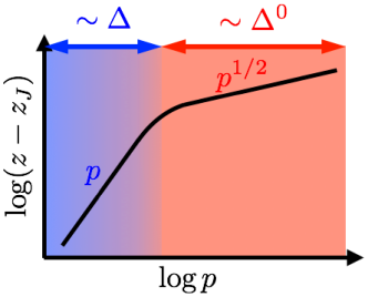
Figure 2: Schematic behavior of the contact number. Near the jamming transition point, $z-z_{J}\propto p$, while $z-z_{J}\propto p^{1/2}$ away from jamming.

From Eqs. (38), (62), and (65), we have

$$k_{R} =\Delta^{2}\frac{K}{\chi}\sim\Delta p.$$ (68)

Finally, by substituting Eq. (65) into Eq. (60), we can calculate $g(h)$ and $P(f)$ at the jamming transition point. Interestingly, the resulting equations are identical to Eqs. (55), meaning that the criticality of $g(h)$ and $P(f)$ is controlled by $\delta z$ only. Because $\delta z>0$ for nonspherical particles, $g(h)$ and $P(f)$ remain finite and regular functions even at the jamming transition point.

6 Vibrational density of states

In this section, we discuss the scaling of the vibrational density of states $D(\omega)$ of the polydisperse perceptron. We focus on the region $\sigma<0$ where the model falls into the same universality class of nonspherical particles, as shown in the previous sections. In the UNSAT phase the ground state is a configuration of the state vectors $\bm{x}$ and $\bm{R}$ that minimizes the potential $V_{N}$. By defining $\rho(\lambda)$ as the eigenvalue distribution of the Hessian of $V_{N}$ computed in the ground state, the density of states is given by

$$D(\omega)=2\omega\rho(\lambda=\omega^{2}).$$ (69)

To calculate $\rho(\lambda)$, we consider a slightly modified interaction potential:

$$V_{N} =\sum_{\mu=1}^{M}\frac{h_{\mu}^{2}}{2}\theta(-h_{\mu})+\frac{k_{R}}{2}\sum_{\mu=1}^{M}R_{\mu}^{2}-\frac{\zeta}{2}\left(\sum_{i=1}^{N}x_{i}^{2}-N\right),$$ (70)

where $\zeta$ denotes the Lagrange multiplier that is needed to impose the spherical constraint $|\bm{x}|^{2}=N$. In the UNSAT phase, the first term of Eq. (70) is a sum over the UNSAT constraints, which are the $Nz$ contacts defined as the gaps that satisfy $\theta(-h_{\mu})=1$. For convenience, we hereafter reassign the index $\mu$ only to these gaps $\mu=1,\cdots Nz$. Note that in the following, we neglect the $(\alpha-z)N$ degrees of freedom $R_{\mu}$ associated to the SAT constraints, such that $\theta(-h_{\mu})=0$. These degrees of freedom are trivially decoupled from the system and, if included, would give rise to a delta function $\delta(\lambda-k_{R})$ in the density of states. Using this convention, we can write a reduced $N(1+z)\times N(1+z)$ Hessian of the potential $V_{N}$ as

$$H_{ij} \equiv\frac{\partial^{2}V_{N}}{\partial x_{i}\partial x_{j}}=\frac{1}{N}\sum_{\mu=1}^{zN}\xi_{i}^{\mu}\xi_{j}^{\mu}-\zeta\delta_{ij},$$

$$Q_{\mu\nu} \equiv\frac{\partial^{2}V_{N}}{\partial R_{\mu}\partial R_{\nu}}=\left[\Delta^{2}+k_{R}\right]\delta_{\mu\nu},$$

$$T_{\mu i} \equiv\frac{\partial^{2}V_{N}}{\partial R_{\mu}\partial x_{i}}=-\frac{\Delta\xi_{i}^{\mu}}{\sqrt{N}}.$$ (71)

We define the Hessian matrix as

$$\mathcal{H} =\begin{pmatrix}H&T\\ T^{t}&Q\end{pmatrix}.$$ (72)

One can calculate the eigenvalue distribution $\rho(\lambda)$ of $\mathcal{H}$ by using the Edwards-Jones formula [57]:

$$\rho(\lambda) \equiv\frac{1}{N+zN}\sum_{k=1}^{N+zN}\delta(\lambda-\lambda_{k})=-\frac{2}{(N+zN)\pi}\lim_{\varepsilon\to 0}{\rm Im}\frac{\partial}{\partial\lambda}\overline{\log Z(\lambda-i\varepsilon)},$$ (73)

where the overline denotes the average over the quenched disorder $\xi_{i}^{\mu}$, and we have introduced a partition function as

$$Z(\lambda) =\int d\bm{u}\exp\left[-\frac{1}{2}\bm{u}\cdot(\lambda I_{N+zN}-\mathcal{H})\cdot\bm{u}\right].$$ (74)

Here $I_{d}$ denotes the $d$-dimensional unit matrix. Due to the mean field nature of the model, we can derive the analytical expression of $\rho(\lambda)$ (see D):

$$\rho(\lambda) =\frac{z-1}{1+z}\delta(\lambda-\Delta^{2}-k_{R})+\mathcal{R}(\lambda),$$

$$\mathcal{R}(\lambda) =\left|\frac{{\rm Im}\sqrt{\prod_{i=1}^{4}(\lambda-\lambda_{i})}}{2\pi(1+z)}\left[\frac{1}{(\lambda-k_{R})(\lambda+\zeta)}-\frac{1}{(\lambda-k_{R})^{2}}+\frac{1}{(\lambda-k_{R})(\lambda-\Delta^{2}-k_{R})}\right]\right|,$$ (75)

where the explicit expressions of $\lambda_{1},\cdots,\lambda_{4}$ are given in D. To calculate $\rho(\lambda)$, one needs to calculate $\zeta$, $z$, and $k_{R}$ for given $p$ and $\Delta$. In the RSB phase, there is a useful relation to express $\zeta$ (see E):

$$\zeta =\frac{1}{1+\Delta^{2}/k_{R}}\left(\sqrt{z}-1\right)^{2}.$$ (76)

To calculate $z$ and $k_{R}$, one should solve the RSB equation numerically, which is a difficult task. Since we are mainly interested in the scaling property of the density of states, here we assume a suitable ansatz for $z$ and $k_{R}$ of the same form discussed in the previous sections. The scaling of $z$ given by Eq. (67), can be satisfied by assuming

$$\delta z =\left(c_{1}p+c_{2}\Delta\right)^{1/2},$$ (77)

where $c_{1}$ and $c_{2}$ are constants. To satisfy Eq. (68), we assume

$$k_{R} =c_{3}\Delta p,$$ (78)

where $c_{3}$ is another constant. Because these constants do not affect the scaling behavior, we set them to $c_{1}=c_{2}=c_{3}=1$. Substituting Eqs. (77) and (78) into Eq. (75), and using Eq. (69), one can calculate $D(\omega)$.

Figure 3: Density of states of the perceptron for $\Delta=10^{-2}$ and $p=10^{-4}$. The black solid line denotes the theoretical result. The green line denotes $D(\omega)\sim\omega^{2}$ scaling. The arrows indicate the characteristic frequencies.

In Fig. 3, we show the typical behavior of $D(\omega)$, which consists of three regions separated by finite gaps:

1. The lowest band is quasi-gapless and ends at $\omega_{0}$. The existence of gapless excitations is a direct consequence of RSB as already discussed for the standard perceptron [26]. The weight of the lowest band is $f_{0}\equiv\int_{0}^{\omega_{0}^{2}}d\lambda\rho(\lambda)=\int_{0}^{\omega_{0}}d\omega D(\omega)=1/(1+z)$.

2. The delta function at $\omega_{1}$. The weight is $f_{1}=(z-1)/(1+z)$.

3. The highest band starting at $\omega_{2}$. The weight of this band is $f_{2}=1/(1+z)$.

Note that $D(\omega)$ is normalized so that $\int_{0}^{\infty}d\omega D(\omega)=f_{0}+f_{1}+f_{2}=1$. The behavior of $D(\omega)$ that we find in the polydisperse spherical perceptron resembles very closely to that obtained in numerical simulations of ellipsoids [42], where again $D(\omega)$ consists of three well-separated regions. To uncover further similarity, we discuss the scaling behavior of the characteristic frequencies, $\omega_{0}$, $\omega_{1}$, and $\omega_{2}$.

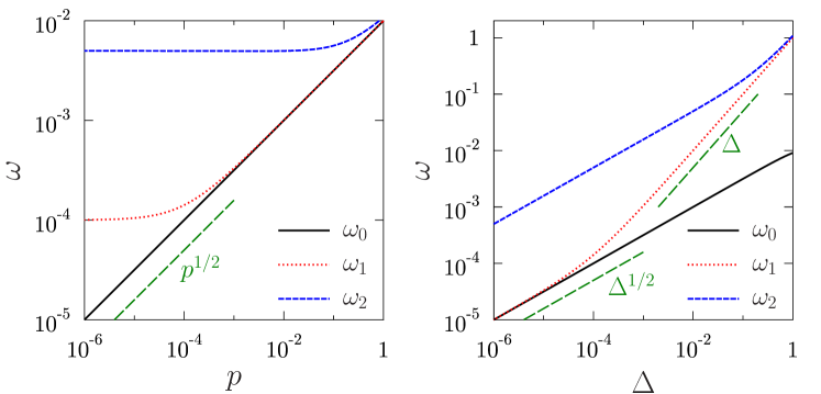
Figure 4: Scaling of the characteristic frequencies near the jamming transition point. The left panel shows the $p$ dependence of the characteristic frequencies for fixed $\Delta=10^{-4}$, while the right panel shows the $\Delta$ dependence for $p=10^{-4}$. The black solid line, red dotted line, and blue dashed lines indicate the theoretical results for $\omega_{0}$, $\omega_{1}$, and $\omega_{2}$, respectively. The green lines are guide for eye.

In Fig. 4, we show the $p$ and $\Delta$ dependence of the characteristic frequencies, from which one can deduce the following scaling behavior:

$$\omega_{0} \sim\Delta^{1/2}p^{1/2}, \omega_{1} \sim\begin{cases}\Delta^{1/2}p^{1/2}&(p\gg\Delta)\\ \Delta&(p\ll\Delta)\end{cases}, \omega_{2} \sim\Delta^{1/2}.$$ (79)

The same scaling can also be obtained directly by the asymptotic analysis of $\lambda_{1},\cdots,\lambda_{4}$. For $p\ll\Delta$ we find the same scaling reported in Ref. [42] for the case of ellipsoids. Instead it seems that the aspect ratios used in Ref. [42] are too large to observe the scaling for $p\gg\Delta$. It would be interesting to redo the numerical simulation to further investigate this case. For the lowest frequency regime, we get that $\rho(\lambda)\sim\sqrt{\lambda}\theta(\lambda)$, which leads to $D(\omega)\sim\omega^{2}$, see Fig. 3 as in the case of the spherical perceptron [26].

7 Summary and discussions

In this manuscript, we constructed a mean field theory for the jamming transition of nonspherical particles based on the analytical solution of the polydisperse spherical perceptron model. This model is an extension of the spherical perceptron model introduced in [32] to study jamming of spherical particles. In order to take into account the particles shape, which results in internal degrees of freedom such as the orientations, we introduced additional internal degrees of freedom in the perceptron model [45]. We can parametrize the asphericity of particles using an additional control parameter $\Delta$. We solved the model through the replica method and we determined the phase diagram and the asymptotic behavior of the gap (and force) distributions near and at the jamming transition point. The resulting generic picture is showed in the left panel of Fig. 5, where we summarize the phase diagram predicted by our theoretical calculation. For $\Delta=0$, which corresponds to spherical particles, the system is isostatic at the jamming point, and the gap and force distributions show a power law behavior [32]. On the contrary, for $\Delta>0$, which corresponds to nonspherical particles of finite asphericity, the system is not isostatic at the jamming transition point, and the gap and force distributions remain regular and finite. In the right panel of Fig. 5, we show the critical exponents of the shear modulus and contact number. Due to the regularity of the distribution function, the critical exponent takes a rather simple value for $\Delta>0$: the shear modulus and contact number are linearly proportional to the proximity to the jamming transition point. On the contrary, they are proportional to the square root of the proximity to the jamming transition point for spherical particles. Thus, the exponent jumps from one-half to one at $\Delta=0$. We also calculated the density of states $D(\omega)$ and found that our model reproduces the scaling behavior of $D(\omega)$ of ellipsoids near the jamming transition point, previously reported in numerical simulations. Our results highlight the specificity of the universality of jamming of spherical particles, which holds only when the asphericity is precisely zero, whereas the universality of nonspherical particles is far more general as it holds no matter how small the asphericity is.

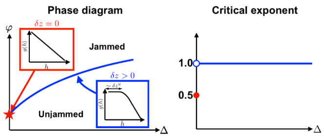
Figure 5: Summary of theoretical results. (left) The putative jamming line as a function of the deviation from sphere $\Delta$. The red star at $\Delta=0$ indicates that the jamming transition point of spherical particles, where the system is isostatic $\delta z=0$ and the gap distribution shows the power law behavior. The blue line for $\Delta>0$ represents the jamming transition point of nonspherical particles, where the system is not isostatic $\delta z>0$ and the power law of the gap distribution is truncated at $h\sim\delta z^{\psi}$. (right) The critical exponent of the shear modulus and the contact number near the jamming transition point. The critical exponent jumps at $\Delta=0$ from $0.5$ to $1.0$.

There are still several important points that deserve further investigation. Here we give a tentative list:

• In previous research, we confirmed our theoretical prediction for the gap distribution function by computer simulation of breathing particles, which belong to the same universality class of nonspherical particles [45]. It would be important to repeat the same analysis for various shapes of nonspherical particles to confirm the absence of criticality also in those cases.

• $D(\omega)$ of nonspherical particles differs dramatically from that of spherical particles. An interesting question is how this difference affects the steady-state rheology near the jamming transition point. For spherical particles, it has been shown that the minimal eigenfrequency of $D(\omega)$ controls the viscosity near the jamming transition point [58]. It would be interesting to extend the theory in Ref. [58] to the present case to study how the rheology of nonspherical particles differs from that of spherical ones.

• For the low frequency regime of the density of states, our mean field model predicts a quadratic scaling $D(\omega)\sim\omega^{2}$. However, in finite dimensions, it has been shown theoretically that spatial heterogeneity modifies the mean-field result below some characteristic frequency, and the quadratic scaling is replaced by a quartic scaling $D(\omega)\sim\omega^{4}$ [59]. This is indeed consistent with numerical observations in breathing particles, which can be considered as nonspherical particles of small asphericity [60]. It would be interesting future work to test if the same quartic scaling holds for ellipsoids and other nonspherical models.

• In this manuscript, we investigated the fully connected mean-field model, which does not have a spatial structure. A natural next step is to include spatial fluctuations and study the divergence of the correlation length near the jamming transition point. This is possible by considering a Kac version of the model, as previously done for the $p$-spin spherical model [61] and hard spheres [62].

• Although the scaling behavior of our model near the jamming transition point is entirely different from that of the original perceptron model, the two models have qualitatively the same phase diagram, in particular, the jamming line is surrounded by the replica symmetric breaking (RSB) line for $\sigma<0$, where the model can be mapped into a particle system. This means that RSB occurs before the jamming transition point is reached. It would be interesting to see if signatures of such a transition are present for models of nonspherical particles in finite dimension.

• Our approach is justified only for small enough asphericity. For larger asphericity, completely new effects may appear such as (partial) orientational ordering, orientational jamming vs. positional jamming, additional many-body correlations, higher order corrections, those of which can not be captured by our model. To discuss those effects, it is tempting to extend the present calculation for the perceptron to more realistic models of nonspherical particles. A possibility in this direction is to solve nonspherical particle models in the large dimensional limit where one can write down the analytical expression of the free energy as a functional of the density of particle positions and angles, as shown in Ref. [63].

Appendix A Full RSB free energy and saddle point equations

Here, we briefly explain the derivation of the replicated free-energy and saddle point equations. For a more complete discussion see Ref. [46].

Substituting a hierarchical replica ansatz [24] into the free energy of Eq. (13), we obtain

$$\begin{split}-\beta f&=\lim_{n\to 0}\frac{\log Z^{n}}{nN}=\frac{1}{2}\left[\log(1-q_{M})+\frac{q_{m}}{\lambda(0)}+\int_{0}^{1}dx\frac{\dot{q}(x)}{\lambda(x)}\right]\\ &-\frac{\alpha}{2}\log\tilde{k}+\alpha\left.\gamma_{q_{m}}*f(0,h)\right|_{h=-\sigma},\end{split}$$ (80)

where the dot denotes derivation with respect to $x$, and

$$\lambda(x) =1-xq(x)-\int_{x}^{1}dyq(y).$$ (81)

The function $f(x,h)$ is obtained as the solution of the Parisi equation [64]:

$$\dot{f}(x,h) =-\frac{1}{2}\dot{q}(x)\left[f^{\prime\prime}(x,h)+xf^{\prime}(x,h)^{2}\right],\ x_{m}<x<x_{M},$$ (82)

with the boundary condition:

$$f(1,h) =\log_{1-q_{M}+\Delta^{2}/\tilde{k}}*e^{-\beta v(h)}.$$ (83)

We assume that for $x\not\in[x_{m},x_{M}]$, $\dot{q}(x)=0$ while $q(x)$ takes a constant value, $q(x)=q_{m}$ for $x\in[0,x_{m})$ and $q(x)=q_{M}$ for $x\in(x_{M},1]$. For $x\in[x_{m},x_{M}]$, $q(x)$ is a monotonic function, and thus one can define the inverse function $x(q)$. Using $x(q)$, Eq. (82) reduces to

$$\dot{f}(q,h)=-\frac{1}{2}\left[f^{\prime\prime}(q,h)+x(q)f^{\prime}(q,h)^{2}\right],$$ (84)

with

$$f(q_{M},h)=\log_{1-q_{M}+\Delta^{2}/\tilde{k}}*e^{-\beta v(h)}.$$ (85)

The replicated free energy is

$$-\beta f[x(q)] =\frac{1}{2}\left[\log(1-q_{M})+\frac{q_{m}}{\lambda(q_{m})}+\int_{q_{m}}^{q_{M}}\frac{dq}{\lambda(q)}\right]-\frac{\alpha}{2}\log\tilde{k}+\alpha\left.\gamma_{q_{m}}*f(q_{m},h)\right|_{h=-\sigma},$$ (86)

where

$$\lambda(q) =1-q_{M}+\int_{q}^{q_{M}}dpx(p).$$ (87)

In order to compute the saddle point for $q(x)$ or equivalently for $x(q)$, one should extremize Eq. (86) w.r.t $x(q)$, with the constraint that $f(q,h)$ satisfies Eq. (84) and (85). To do this one can introduce the Lagrange multiplier $P(q,h)$ [54] as,

$$-\beta f[x(q)] =\frac{1}{2}\left[\log(1-q_{M})+\frac{q_{m}}{\lambda(q_{m})}+\int_{q_{m}}^{q_{M}}\frac{dq}{\lambda(q)}\right]-\frac{\alpha}{2}\log\tilde{k}+\alpha\left.\gamma_{q_{m}}*f(q_{m},h)\right|_{h=-\sigma}$$

$$-\alpha\int dhP(q_{M},h)\left[f(q_{M},h)-\log\gamma_{1-q_{M}+\Delta^{2}/\tilde{k}}*e^{-\beta v(h)}\right]$$

$$+\alpha\int dh\int_{q_{m}}^{q_{M}}dqP(q,h)\left\{\dot{f}(q,h)+\frac{1}{2}\left[f^{\prime\prime}(q,h)+x(q)f^{\prime}(q,h)^{2}\right]\right\}.$$ (88)

Note that the saddle point conditions for $P(q,h)$ and $P(q_{M},h)$ correctly reproduce Eq. (85) and (83), respectively. The equations for the Lagrange multiplier $P(q,h)$ is obtained taking the functional derivatives w.r.t. $f(q,h)$ and $f(q_{m},h)$:

$$P(q_{m},h) =\gamma_{q_{m}}(h+\sigma),$$

$$\dot{P}(q_{M},h) =\frac{1}{2}\left[P^{\prime\prime}(q,h)-2x(q)\left(P(q,h)f^{\prime}(q,h)\right)^{\prime}\right],\ q_{m}<q<q_{M}.$$ (89)

The saddle point condition for $x(q)$ is

$$\frac{q_{m}}{\lambda(q_{m})^{2}}+\int_{q_{m}}^{q}\frac{dp}{\lambda(p)^{2}}=\alpha\int dhP(q,h)f^{\prime}(q,h)^{2}.$$ (90)

In the continuous RSB phase, $x(q)$ is a continuous function for $x\in[q_{m},q_{M}]$, which allows us to calculate derivation of Eq. (90) w.r.t $q$. The first and second derivatives lead to

$$\frac{1}{\lambda(q)^{2}} =\alpha\int dhP(q,h)f^{\prime\prime}(q,h)^{2},$$ (91)

$$x(q) =\frac{\lambda(q)}{2}\frac{\int dhP(q,h)f^{\prime\prime\prime}(q,h)^{2}}{\int dhP(q,h)\left[f^{\prime\prime}(q,h)^{2}+\lambda(q)f^{\prime\prime}(q,h)^{3}\right]}.$$ (92)

Also, the spherical constraint $\sum_{\mu=1}^{M}R_{\mu}^{2}=M$, gives the last saddle point equation for $\tilde{k}$

$$1 =\frac{1}{\tilde{k}}+\frac{\Delta^{2}}{\tilde{k}^{2}}\int dhP(q_{M},h)\left[f^{\prime\prime}(q_{M},h)+\left(f^{\prime}(q_{M},h)\right)^{2}\right].$$ (93)

Appendix B Replica symmetric analysis in the unjammed phase

Here we investigate the replica symmetric (RS) saddle point equations in the unjammed phase. In this case one has that $e^{-\beta v(h)}=\theta(h)$ so that

$$f_{\rm RS}(q,h)=\log\gamma_{1-q+\Delta^{2}/\tilde{k}}\theta(h)=\log\Theta\left(\frac{h}{\sqrt{2(1-q+\Delta^{2}/\tilde{k})}}\right),$$ (94)

where $\Theta(x)=({\rm erf}(x)+1)/2$. Approaching the jamming point one has that $q\to 1$ and $\tilde{k}\to\infty$. In this limit, using the asymptotic expansion of the error function, we can show that

$$f_{RS}(q,h)\sim-\frac{h^{2}}{2(1-q+\Delta^{2}/\tilde{k})}\theta(-h).$$ (95)

Substituting this expression into Eqs. (28) and Eq. (93), we obtain

$$\tilde{k} \sim\frac{\Delta}{(1-q)\sqrt{\alpha}}.$$ (96)

and

$$\alpha_{J}=\left(\frac{1}{\sqrt{G(\sigma)}-\Delta}\right)^{2}.$$ (97)

which coincides with Eq. (36) obtained from the analysis in the jammed phase.

Appendix C Scaling in the unjammed phase

Here we discuss the scaling behavior when approaching to the jamming transition point from the unjammed phase.

C.1 Failure of the critical solution

We first show that the critical jamming solution for the spherical perceptron does not work for the nonspherical perceptron model when $\Delta>0$. For this purpose, we introduce the following scaling variables:

$$y(q) =\varepsilon^{-1}x(q),$$

$$\hat{f}(q,h) =\varepsilon f(q,h),$$

$$\hat{\pi}(q) =\varepsilon^{-1}\left(\lambda(q)+\frac{\Delta^{2}}{\tilde{k}}\right),$$ (98)

where $\varepsilon$ is the linear distance from the jamming transition point. In the critical solution [46], one assumes

$$1-q_{M} \sim\varepsilon^{\kappa}, \frac{\tilde{k}}{\Delta^{2}} \sim\varepsilon^{-\kappa},$$ (99)

$$y(q) \sim y_{J}(1-q+\Delta^{2}/\tilde{k})^{-1/\kappa},$$

$$P(q,h) \sim\begin{cases}(1-q+\Delta^{2}/\tilde{k})^{(1-\kappa)/\kappa}p_{-}\left[h(1-q+\Delta^{2}/\tilde{k})^{(1-\kappa)/\kappa}\right]&h\sim-(1-q+\Delta^{2}/\tilde{k})^{(\kappa-1)/\kappa},\\ (1-q+\Delta^{2}/\tilde{k})^{-a/\kappa}p_{0}\left(\frac{h}{\sqrt{1-q+\Delta^{2}/\tilde{k}}}\right)&\left|h\right|\sim\sqrt{1-q+\Delta^{2}/\tilde{k}}\\ p_{+}(h)&h\gg\sqrt{1-q+\Delta^{2}/\tilde{k}},\end{cases}$$ (100)

and

$$m(q,h) =\hat{\pi}(q)\hat{f}^{\prime}(q,h)=-\sqrt{1-q+\Delta^{2}/\tilde{k}}\mathcal{M}\left(\frac{h}{\sqrt{1-q+\Delta^{2}/\tilde{k}}}\right),$$

$$\mathcal{M}(t\to\infty) =0,\ \mathcal{M}(t\to-\infty)=t,$$ (101)

where

$$\kappa =1.41574, a =1-\frac{\kappa}{2}.$$ (102)

Substituting these relations into Eq. (93), we get

$$1 \sim\frac{\Delta^{2}}{\tilde{k}^{2}}\int dhP(1,h)f^{\prime}(1,h)^{2}=\frac{\Delta^{2}}{\tilde{k}^{2}\varepsilon^{2}\hat{\pi}(1)^{2}}\int dhP(1,h)m(1,h)^{2},$$ (103)

which leads to

$$\Delta^{2}\sim\varepsilon^{2\kappa-2}\int_{-\infty}^{0}dtp_{-}(t)t^{2}.$$ (104)

This equation can be satisfied only when $\Delta=0$, i.e., in the case of the standard perceptron. A similar equation can be also obtained on approaching to the jamming transition from the jammed phase. We deduce that the critical jamming solution is inconsistent when $\Delta>0$.

C.2 Scaling solution for $\Delta>0$

The jamming scaling for $\Delta>0$ is describe by the regular full RSB solution. We define the scaling solutions as

$$1-q_{M} =\varepsilon,$$

$$\tilde{k} =\frac{\Delta^{2}}{\varepsilon}K.$$ (105)

For $\varepsilon\ll 1$, we have

$$f(1,h)\sim-\frac{h^{2}}{\varepsilon(1+1/K)}\theta(-h).$$ (106)

Also we assume that $P(q,h)$ is a regular and finite function. Then, Eq. (93) reduces to

$$1=\frac{\Delta^{2}}{\tilde{k}^{2}}\int dhP(1,h)f^{\prime}(1,h)^{2}\sim\frac{1}{\Delta^{2}(1+K)^{2}}\int_{-\infty}^{0}dhP(1,h)h^{2}.$$ (107)

Thus, the regular scaling solution gives a well-defined expression in the $\varepsilon\to 0$ limit, unlike the critical scaling. Similarly, the pressure $p$ can be obtained from

$$p =\frac{1}{\alpha}\frac{df}{d\sigma}=T\int dhP(1,h)f^{\prime}(1,h)\sim\frac{T}{\varepsilon(1+1/K)}\int_{-\infty}^{0}dhP(1,h)h,$$ (108)

which implies that $p\sim\varepsilon^{-1}$. Combining this with Eqs. (105), we can determine the pressure dependence of $q_{M}$ and $\tilde{k}$ for $p\ll 1$:

$$1-q_{M} \sim p^{-1}, \tilde{k} \sim p.$$ (109)

Appendix D Derivation of the eigenvalue distribution

We want to compute the eigenvalue distribution $\rho(\lambda)$ of the $(N+zN)\times(N+zN)$ dimensional Hessian defined by:

$$\mathcal{H} =\begin{pmatrix}H&T\\ T^{t}&Q\end{pmatrix},$$ (110)

where

$$H_{ij} \equiv\frac{\partial^{2}V_{N}}{\partial x_{i}\partial x_{j}}=\frac{1}{N}\sum_{\mu=1}^{zN}\xi_{i}^{\mu}\xi_{j}^{\mu}-\zeta\delta_{ij},$$

$$Q_{\mu\nu} \equiv\frac{\partial^{2}V_{N}}{\partial R_{\mu}\partial R_{\nu}}=\left[\Delta^{2}+k_{R}\right]\delta_{\mu\nu},$$

$$T_{\mu i} \equiv\frac{\partial^{2}V_{N}}{\partial R_{\mu}\partial x_{i}}=-\frac{\Delta\xi_{i}^{\mu}}{\sqrt{N}},$$ (111)

for $i,j=1,\cdots,N$ and $\mu,\nu=1,\cdots,zN$. We perform the computation using the Edwards-Jones formula [57]:

$$\rho(\lambda) \equiv\frac{1}{N+zN}\sum_{k=1}^{N+zN}\delta(\lambda-\lambda_{k})=-\frac{2}{(N+zN)\pi}\lim_{\varepsilon\to 0}{\rm Im}\frac{\partial}{\partial\lambda}\overline{\log Z(\lambda-i\varepsilon)},$$ (112)

where the overline denotes the average over the quenched disorder $\xi_{i}^{\mu}$, and we have introduced the partition function as

$$Z(\lambda) =\int d\bm{u}\exp\left[-\frac{1}{2}\bm{u}\cdot(\lambda I_{N+zN}-\mathcal{H})\cdot\bm{u}\right].$$ (113)

Here $I_{d}$ denotes the $d$-dimensional identity matrix. Performing the Gaussian integration we get

$$\log Z(\lambda) =-\frac{1}{2}\log\det\left[\lambda I-\mathcal{H}\right]$$

$$=-\frac{1}{2}\left\{\log\det(\lambda I_{zN}-Q)+\log\det(\lambda I_{N}-H-T^{t}(\lambda I_{zN}-Q)^{-1}T)\right\}$$

$$=-\frac{1}{2}\left\{Nz\log(\lambda-\Delta^{2}-k_{R}))+\log\det A\right\},$$ (114)

where we have introduced a $N\times N$ matrix as

$$A_{ij} =(\lambda+\zeta)\delta_{ij}-\frac{a(\lambda)}{N}\sum_{\mu=1}^{Nz}\xi_{i}^{\mu}\xi_{j}^{\mu},$$

$$a(\lambda) =\left(1+\frac{\Delta^{2}}{\lambda-\Delta^{2}-k_{R}}\right).$$ (115)

Replacing the quenched average by the annealed one and using the saddle point method, we can show that

$$\overline{\log\det A} \approx\log\overline{\det A}$$

$$\sim N(\lambda+\zeta)q-N\log q+Nz\log(1-a(\lambda)q),$$ (116)

where $q=N^{-1}\sum_{i=1}^{N}u_{i}^{2}$ is to be determined by the saddle point condition:

$$\lambda+\zeta-\frac{1}{q}-z\frac{a(\lambda)}{1-\alpha(\lambda)q}=0.$$ (117)

This can be solved for $q$:

$$q(\lambda) =\frac{1}{2a(\lambda)}+\frac{1-z}{2(\lambda+\zeta)}\pm\frac{\sqrt{\left[\lambda+\zeta-a(\lambda)(1+\sqrt{z})^{2}\right]\left[\lambda+\zeta-a(\lambda)(1-\sqrt{z})^{2}\right]}}{2(\lambda+\zeta)a(\lambda)},$$ (118)

where the sign is to be chosen so that $\rho(\lambda)$ is positive and normalized. Substituting Eqs. (114) and (116) into Eq. (73), we have

$$\rho(\lambda) =\frac{1}{\pi}\lim_{\varepsilon\to 0}{\rm Im}G(\lambda-i\varepsilon),$$

$$G(\lambda) \equiv\frac{z}{1+z}\frac{1}{\lambda-\Delta^{2}-k_{R}}+\frac{1}{1+z}q(\lambda)-\frac{z}{1+z}\frac{a^{\prime}(\lambda)}{1-a(\lambda)q(\lambda)}q(\lambda).$$ (119)

After a straightforward calculation, we finally get

$$\rho(\lambda) =\frac{1-z}{1+z}\theta(1-z)\delta(\lambda+\zeta)+\frac{z-1}{1+z}\theta(z-1)\delta(\lambda-\Delta^{2}-k_{R})$$

$$+\left|\frac{{\rm Im}\sqrt{\prod_{i=1}^{4}(\lambda-\lambda_{i})}}{2\pi(1+z)}\left[\frac{1}{(\lambda-k_{R})(\lambda+\zeta)}-\frac{1}{(\lambda-k_{R})^{2}}+\frac{1}{(\lambda-k_{R})(\lambda-\Delta^{2}-k_{R})}\right]\right|,$$ (120)

where

$$\lambda_{1} =\frac{1}{2}\left[(1-\sqrt{z})^{2}+k_{R}+\Delta^{2}-\zeta-\sqrt{\left\{(1-\sqrt{z})^{2}+k_{R}+\Delta^{2}-\zeta\right\}^{2}-4\left\{(1-\sqrt{z})^{2}k_{R}-(k_{R}+\Delta^{2})\zeta\right\}}\right],$$

$$\lambda_{2} =\frac{1}{2}\left[(1+\sqrt{z})^{2}+k_{R}+\Delta^{2}-\zeta-\sqrt{\left\{(1+\sqrt{z})^{2}+k_{R}+\Delta^{2}-\zeta\right\}^{2}-4\left\{(1+\sqrt{z})^{2}k_{R}-(k_{R}+\Delta^{2})\zeta\right\}}\right],$$

$$\lambda_{3} =\frac{1}{2}\left[(1-\sqrt{z})^{2}+k_{R}+\Delta^{2}-\zeta+\sqrt{\left\{(1-\sqrt{z})^{2}+k_{R}+\Delta^{2}-\zeta\right\}^{2}-4\left\{(1-\sqrt{z})^{2}k_{R}-(k_{R}+\Delta^{2})\zeta\right\}}\right],$$

$$\lambda_{4} =\frac{1}{2}\left[(1+\sqrt{z})^{2}+k_{R}+\Delta^{2}-\zeta+\sqrt{\left\{(1+\sqrt{z})^{2}+k_{R}+\Delta^{2}-\zeta\right\}^{2}-4\left\{(1+\sqrt{z})^{2}k_{R}-(k_{R}+\Delta^{2})\zeta\right\}}\right].$$ (121)

Since $z>1$ in the RSB jammed phase, Eq. (120) can be slightly simplified as

$$\rho(\lambda) =\frac{z-1}{1+z}\delta(\lambda-\Delta^{2}-k_{R})$$

$$+\left|\frac{{\rm Im}\sqrt{\prod_{i=1}^{4}(\lambda-\lambda_{i})}}{2\pi(1+z)}\left[\frac{1}{(\lambda-k_{R})(\lambda+\zeta)}-\frac{1}{(\lambda-k_{R})^{2}}+\frac{1}{(\lambda-k_{R})(\lambda-\Delta^{2}-k_{R})}\right]\right|.$$ (122)

Appendix E Calculation of $\zeta$

We here determine the Lagrange multiplier $\zeta$ introduced in Sec. 3. For this purpose, we rewrite the free energy Eq. (88) as

$$-\beta f[x(q)] =\frac{1}{2}\left[\log(q_{d}-q_{M})+\frac{q_{m}}{\lambda(q_{m})}+\int_{q_{m}}^{q_{M}}\frac{dq}{\lambda(q)}\right]-\frac{\alpha}{2}\log\tilde{k}+\alpha\left.\gamma_{q_{m}}*f(q_{m},h)\right|_{h=-\sigma}$$

$$-\alpha\int dhP(q_{M},h)\left[f(q_{M},h)-\log\gamma_{q_{d}-q_{M}+\Delta^{2}/\tilde{k}}*e^{-\beta v(h)}\right]$$

$$+\alpha\int dh\int_{q_{m}}^{q_{M}}dqP(q,h)\left\{\dot{f}(q,h)+\frac{1}{2}\left[f^{\prime\prime}(q,h)+x(q)f^{\prime}(q,h)^{2}\right]\right\}$$

$$+\frac{\beta\zeta N}{2}\left(q_{d}-1\right),$$ (123)

where $q_{d}=N^{-1}\sum_{i}x_{i}^{2}$. The saddle point condition for $q_{d}$ leads to

$$\frac{1}{2}\left(\frac{1}{q_{d}-q_{M}}-\frac{q_{m}}{\lambda(q_{m})^{2}}-\int_{q_{m}}^{q_{M}}\frac{dp}{\lambda(p)^{2}}\right)+\alpha\int dhP(q_{M},h)\frac{\partial}{\partial q_{d}}\log\gamma_{q_{d}-q_{M}+\Delta^{2}/\tilde{k}}*e^{-\beta v(h)}$$

$$+\frac{\beta\zeta}{2}=0$$ (124)

After some manipulations, this can be rewritten as

$$\beta\zeta =-\frac{1}{q_{d}-q_{M}}+\alpha\int dhP(q_{M},h)f^{\prime\prime}(q_{M},h).$$ (125)

Substituting $q_{M}\sim q_{d}-T\chi$, $f(q_{M},h)\sim-\beta h^{2}\theta(-h)/(1+\chi+\Delta^{2}/k_{R})$, and taking the zero temperature limit $T\to 0$, we get

$$\zeta =\frac{1+\Delta^{2}/k_{R}}{\chi}=\frac{(\sqrt{z}-1)^{2}}{1+\Delta^{2}/k_{R}}.$$ (126)

References

References

- [1] Van Hecke M 2009 J. Phys. Condens. Matter 22 033101
- [2] Torquato S and Stillinger F H 2010 Rev. Mod. Phys. 82(3) 2633–2672
- [3] Bernal J and Mason J 1960 Nature 188 910
- [4] Durian D J 1995 Phys. Rev. Lett. 75 4780
- [5] O’Hern C S, Silbert L E, Liu A J and Nagel S R 2003 Phys. Rev. E 68(1) 011306
- [6] Zhang Z, Xu N, Chen D T, Yunker P, Alsayed A M, Aptowicz K B, Habdas P, Liu A J, Nagel S R and Yodh A G 2009 Nature 459 230
- [7] Karayiannis N C, Foteinopoulou K and Laso M 2009 J. Chem. Phys. 130 164908
- [8] Donev A, Cisse I, Sachs D, Variano E A, Stillinger F H, Connelly R, Torquato S and Chaikin P M 2004 Science 303 990–993
- [9] Jaoshvili A, Esakia A, Porrati M and Chaikin P M 2010 Phys. Rev. Lett. 104(18) 185501
- [10] Bi D, Lopez J, Schwarz J and Manning M L 2015 Nature Physics 11 1074
- [11] Donev A, Torquato S and Stillinger F H 2005 Phys. Rev. E 71(1) 011105
- [12] Lerner E, Düring G and Wyart M 2013 Soft Matter 9 8252–8263
- [13] Wyart M 2012 Phys. Rev. Lett. 109(12) 125502
- [14] Silbert L E, Liu A J and Nagel S R 2005 Phys. Rev. Lett. 95(9) 098301
- [15] Hexner D, Liu A J and Nagel S R 2018 Physical review letters 121 115501
- [16] Hexner D, Urbani P and Zamponi F 2019 arXiv preprint arXiv:1902.00630
- [17] Wyart M, Nagel S and Witten T 2005 Europhysics Letters 72 486–492
- [18] Wyart M 2012 Phys. Rev. Lett. 109(12) 125502
- [19] Mézard M and Parisi G 2012 Glasses and replicas Structural glasses and supercooled liquids: theory, experiment and applications ed Wolynes P G and Lubchenko V (Wiley & Sons) (Preprint arXiv:0910.2838)
- [20] Parisi G and Zamponi F 2010 Rev. Mod. Phys. 82(1) 789–845
- [21] Singh Y, Stoessel J P and Wolynes P G 1985 Phys. Rev. Lett. 54 1059–1062
- [22] Kirkpatrick T R and Wolynes P G 1987 Physical Review A 35 3072–3080
- [23] Kirkpatrick T R and Thirumalai D 1989 Journal of Physics A: Mathematical and General 22 L149
- [24] Mézard M, Parisi G and Virasoro M 1987 Spin glass theory and beyond: An Introduction to the Replica Method and Its Applications vol 9 (World Scientific Publishing Company)
- [25] Kurchan J, Parisi G, Urbani P and Zamponi F 2013 J. Phys. Chem. B 117 12979–12994
- [26] Franz S, Parisi G, Urbani P and Zamponi F 2015 PNAS 112 14539–14544
- [27] Altieri A, Franz S and Parisi G 2016 J. Stat. Mech. Theory Exp. 2016 093301
- [28] Charbonneau P, Kurchan J, Parisi G, Urbani P and Zamponi F 2014 Nat. Commun. 5 3725
- [29] Charbonneau P, Kurchan J, Parisi G, Urbani P and Zamponi F 2014 Journal of Statistical Mechanics: Theory and Experiment 2014 P10009
- [30] Charbonneau P, Corwin E I, Parisi G and Zamponi F 2015 Phys. Rev. Lett. 114(12) 125504
- [31] Charbonneau P, Kurchan J, Parisi G, Urbani P and Zamponi F 2017 Annu. Rev. Condens. Matter Phys. 8 265–288
- [32] Franz S and Parisi G 2016 J. Phys. A 49 145001
- [33] Monasson R, Zecchina R, Kirkpatrick S, Selman B and Troyansky L 1999 Nature 400 133
- [34] Mézard M, Parisi G and Zecchina R 2002 Science 297 812–815
- [35] Krzakała F, Montanari A, Ricci-Tersenghi F, Semerjian G and Zdeborová L 2007 PNAS 104 10318–10323
- [36] Mailman M, Schreck C F, O’Hern C S and Chakraborty B 2009 Phys. Rev. Lett. 102(25) 255501
- [37] Williams S R and Philipse A P 2003 Phys. Rev. E 67(5) 051301
- [38] Jiao Y, Stillinger F H and Torquato S 2010 Phys. Rev. E 81(4) 041304
- [39] Delaney G W and Cleary P W 2010 EPL 89 34002
- [40] VanderWerf K, Jin W, Shattuck M D and O’Hern C S 2018 Phys. Rev. E 97(1) 012909
- [41] Boromand A, Signoriello A, Ye F, O’Hern C S and Shattuck M D 2018 Phys. Rev. Lett. 121(24) 248003
- [42] Schreck C F, Mailman M, Chakraborty B and O’Hern C S 2012 Phys. Rev. E 85(6) 061305
- [43] Donev A, Connelly R, Stillinger F H and Torquato S 2007 Phys. Rev. E 75(5) 051304
- [44] Baule A, Mari R, Bo L, Portal L and Makse H A 2013 Nat. Commun. 4 2194
- [45] Brito C, Ikeda H, Urbani P, Wyart M and Zamponi F 2018 PNAS 115 11736–11741
- [46] Franz S, Parisi G, Sevelev M, Urbani P and Zamponi F 2017 SciPost Phys. 2(3) 019
- [47] Rosenblatt F 1958 Psychol. Rev. 65 386
- [48] Gardner E 1988 Journal of physics A: Mathematical and general 21 257
- [49] Gardner E and Derrida B 1988 Journal of Physics A: Mathematical and general 21 271
- [50] Nishimori H 2001 Statistical physics of spin glasses and information processing: an introduction vol 111 (Clarendon Press)
- [51] Brito C, Lerner E and Wyart M 2018 Physical Review X 8 031050
- [52] Franz S, Sclocchi A and Urbani P 2019 arXiv preprint arXiv:1902.08243
- [53] Mézard M, Parisi G and Virasoro M 1987 Spin glass theory and beyond: An Introduction to the Replica Method and Its Applications vol 9 (World Scientific Publishing Company)
- [54] Sommers H J and Dupont W 1984 Journal of Physics C: Solid State Physics 17 5785
- [55] Gardner E and Derrida B 1988 Journal of Physics A: Mathematical and general 21 271
- [56] Schreck C F, Xu N and O’Hern C S 2010 Soft Matter 6 2960–2969
- [57] Edwards S F and Jones R C 1976 J. Phys. A 9 1595
- [58] Lerner E, Düring G and Wyart M 2012 PNAS 109 4798–4803
- [59] Ikeda H 2019 Phys. Rev. E 99(5) 050901 URL https://link.aps.org/doi/10.1103/PhysRevE.99.050901
- [60] Kapteijns G, Ji W, Brito C, Wyart M and Lerner E 2019 Phys. Rev. E 99(1) 012106
- [61] Franz S and Montanari A 2007 J. Phys. A 40 F251
- [62] Ikeda H and Ikeda A 2015 EPL 111 40007
- [63] Yoshino H 2018 arXiv preprint arXiv:1807.04095
- [64] Parisi G 1980 Journal of Physics A: Mathematical and General 13 L115