Gravitational waves from the minimal gauged $U(1)_{B-L}$ model

Abstract

An additional $U(1)$ gauge interaction is one of the promising extensions of the standard model of particle physics. Among others, the $U(1)_{B-L}$ gauge symmetry is particularly interesting because it addresses the origin of Majorana masses of right-handed neutrinos, which naturally leads to tiny light neutrino masses through the seesaw mechanism. We show that, based on the minimal $U(1)_{B-L}$ model, the symmetry breaking of the extra $U(1)$ gauge symmetry with its minimal Higgs sector in the early universe can exhibit the first-order phase transition and hence generate a large enough amplitude of stochastic gravitational wave radiation that is detectable in future experiments.

I Introduction

The standard model (SM) of particle physics based on the gauge group $SU(3)_{C}\times SU(2)_{L}\times U(1)_{Y}$ successfully describes most of the elementary particle phenomena below the TeV scale. Nevertheless, an additional $U(1)$ gauge interaction is one of promising extensions of the SM. As a minimal extension of the SM, we may consider models based on the gauge group $SU(3)_{C}\times SU(2)_{L}\times U(1)_{Y}\times U(1)_{B-L}$ Mohapatra:1980qe ; Mohapatra:1980 , where the $U(1)_{B-L}$ (baryon number minus lepton number) gauge symmetry is supposed to be broken at a high energy scale. In this model with a conventional $U(1)_{B-L}$ charge assignment, the gauge and gravitational anomaly cancellations require us to introduce three right-handed (RH) neutrinos whose Majorana masses are generated by the spontaneous breakdown of the $U(1)_{B-L}$ gauge symmetry. With Yukawa interactions between left-handed and RH neutrinos, the observed tiny neutrino masses is naturally explained by the so-called seesaw mechanism with the heavy Majorana RH neutrinos SeesawY ; SeesawG ; SeesawM . If the energy scale of the $U(1)_{B-L}$ symmetry breaking is much higher than the TeV scale as is often assumed, it is very difficult for any collider experiments to test the mechanism of the symmetry breaking and the RH neutrino mass generation.

In Ref. Okada:2018xdh , two of the present authors showed that the $U(1)_{B-L}$ symmetry breaking with a simple extended $U(1)_{B-L}$ Higgs sector at such a high energy below about $10^{7}$ GeV scale can be probed by the detection of a gravitational wave (GW) and its energy scale dependence in the spectrum. For a similar work, see, e.g., Ref. Brdar:2018num . Although it has been pointed out that GWs generated by a first-order phase transition at a temperature about $10^{7}$ GeV could be in reach of future experiments Grojean:2006bp ; Dev:2016feu ; Balazs:2016tbi , the possibility has not been explicitly demonstrated for the specific high scale $U(1)_{B-L}$ model well motivated by neutrino physics before the work in Ref. Okada:2018xdh . In this previous work, the Higgs sector was extended so that a trilinear interaction of scalar fields in the tree level potential can be introduced as in Ref. Chao:2017ilw , which play a crucial role to trigger the first-order phase transition.

In this paper, we investigate GWs from the first-order phase transition associated with the spontaneous $U(1)_{B-L}$ gauge symmetry breaking within the minimal model context. If a first-order phase transition happens in the early universe, the dynamics of bubble collision Turner:1990rc ; Kosowsky:1991ua ; Kosowsky:1992rz ; Turner:1992tz ; Kosowsky:1992vn followed by turbulence of the plasma Kamionkowski:1993fg ; Kosowsky:2001xp ; Dolgov:2002ra ; Gogoberidze:2007an ; Caprini:2009yp and sonic waves generate GWs Hindmarsh:2013xza ; Hindmarsh:2015qta ; Hindmarsh:2016lnk , which can be detected by the future experiments, such as the eLISA Seoane:2013qna , the Big Bang Observer (BBO) Harry:2006fi , DECi-hertz Interferometer Observatory (DECIGO) Seto:2001qf and Advanced LIGO (aLIGO) Harry:2010zz .

This paper is organized as follows: In the next section, we introduce formulas we adopt to describe the spectrum of GWs generated by a cosmological first-order phase transition. In Sec. III, we describe the minimal $U(1)_{B-L}$ model and then derive the resultant GWs spectrum by estimating the latent heat and the transition timescale of the phase transition. We also discuss model parameter dependence of the GWs spectrum. In the last section, we summarize our results.

II GW generation by cosmological first-order phase transition

In this section, we briefly summarize the properties of GWs produced by three main GW production processes and mechanisms: bubble collisions, turbulence Kamionkowski:1993fg , and sound waves after bubble collisions Hindmarsh:2013xza . See, for instance, Refs. Caprini:2018mtu ; Mazumdar:2018dfl for a recent review. The GW spectrum generated by a first-order phase transition of a Higgs field critically depends on two quantities: the ratio of the latent heat energy to the radiation energy density $\rho_{\mathrm{rad}}$, which is expressed by a parameter $\alpha$, and the transition speed $\beta$ defined below. In this section, we give definitions of those parameters and the fitting formula of the GW spectrum.

II.1 Scalar potential parameters related to the GW spectrum

A phase transition is induced by a scalar field $\phi$ in the radiation dominated universe with temperature $T$. At the moment of a first-order phase transition, the latent energy density is given by

$$\epsilon=\left.\left(V-T\frac{\partial V}{\partial T}\right)\right|_{\{\phi_{\mathrm{high}},T_{\star}\}}-\left.\left(V-T\frac{\partial V}{\partial T}\right)\right|_{\{\phi_{\mathrm{low}},T_{\star}\}},$$ (1)

where $\phi_{\mathrm{high}(\mathrm{low})}$ denotes the field value of $\phi$ at the high (low) vacuum. Here and hereafter, quantities with the subscript $\star$ denote those at the time when the phase transition takes place Huber:2008hg . On the other hand, the radiation energy density is given by

$$\rho_{\mathrm{rad}}=\frac{\pi^{2}g_{*}}{30}T^{4},$$ (2)

with $g_{*}$ being the total number of relativistic degrees of freedom in the thermal plasma. The parameter $\alpha$ is defined by

$$\alpha\equiv\frac{\epsilon}{\rho_{\mathrm{rad}}}.$$ (3)

The bubble nucleation rate per unit volume at a finite temperature is given by

$$\Gamma(T)=\Gamma_{0}e^{-S(T)}\simeq\Gamma_{0}e^{-S^{3}_{E}(T)/T}.$$ (4)

Here, $\Gamma_{0}$ is a coefficient of the order of the transition energy scale, $S$ is the action in the four-dimensional Minkowski space, and $S^{3}_{E}$ is the three-dimensional Euclidean action Turner:1992tz . The transition timescale is characterized by a dimensionless parameter

$$\frac{\beta}{H_{\star}}\simeq\left.T\frac{dS}{dT}\right|_{T_{\star}}=\left.T\frac{d(S^{3}_{E}/T)}{dT}\right|_{T_{\star}},$$ (5)

with

$$\beta\equiv-\left.\frac{dS}{dt}\right|_{t_{\star}}.$$ (6)

II.2 GW spectrum

Here, we briefly note formulas of generated GW by each of three sources: bubble collisions, turbulence, and sound waves after bubble collisions. The final spectrum is expressed, by taking the sum of all three, as

$$\Omega_{GW}(f)=\Omega_{GW}^{\mathrm{coll}}(f)+\Omega_{GW}^{\mathrm{sw}}(f)+\Omega_{GW}^{\mathrm{turb}}(f),$$ (7)

in terms of the density parameter. For information, we find that the bubble collision contribution is negligible, the sound wave is the dominant source, and turbulence gives a high frequency tail in the spectrum, as GWs generated by a first-order phase transition in many other models.

II.2.1 Bubble collisions

The peak frequency and the peak amplitude of GWs generated by bubble collisions are, under the envelope approximation and for $\beta/H_{\star}\gg 1$ Kosowsky:1992vn , expressed by

$$f_{\mathrm{peak}} \simeq 17\left(\frac{f_{\star}}{\beta}\right)\left(\frac{\beta}{H_{\star}}\right)\left(\frac{T_{\star}}{10^{8}\,\mathrm{GeV}}\right)\left(\frac{g_{*}}{100}\right)^{1/6}\mathrm{Hz},$$ (8)

$$h^{2}\Omega_{GW}^{\mathrm{coll}}(f_{\mathrm{peak}}) \simeq 1.7\times 10^{-5}\kappa^{2}\Delta\left(\frac{\beta}{H_{\star}}\right)^{-2}\left(\frac{\alpha}{1+\alpha}\right)^{2}\left(\frac{g_{*}}{100}\right)^{-1/3},$$ (9)

with

$$\Delta =\frac{0.11v_{b}^{3}}{0.42+v_{b}^{2}},$$ (10)

$$\frac{f_{\star}}{\beta} =\frac{0.62}{1.8-0.1v_{b}+v_{b}^{2}},$$ (11)

where $v_{b}$ is the bubble wall velocity. Here, the efficiency factor ($\kappa$) is given by Kamionkowski:1993fg

$$\kappa=\frac{1}{1+A\alpha}\left(A\alpha+\frac{4}{27}\sqrt{\frac{3\alpha}{2}}\right),$$ (12)

with $A=0.715$. The full GW spectrum can be well fitted by Huber:2008hg

$$\Omega_{GW}^{\mathrm{coll}}(f)=\Omega_{GW}^{\mathrm{coll}}(f_{\mathrm{peak}})\frac{(a+b)f_{\mathrm{peak}}^{b}f^{a}}{bf_{\mathrm{peak}}^{a+b}+af^{a+b}},$$ (13)

with numerical factors $a\in[2.66,2.82]$ and $b\in[0.90,1.19]$. We adopt the values of $(a,b,v_{b})=(2.7,1.0,0.6)$ in our analysis.

II.2.2 Sound waves

The peak frequency and the peak amplitude of GWs generated by sound waves are expressed by Hindmarsh:2013xza ; Hindmarsh:2015qta

$$f_{\mathrm{peak}} \simeq 19\frac{1}{v_{b}}\left(\frac{\beta}{H_{\star}}\right)\left(\frac{T_{\star}}{10^{8}\,\mathrm{GeV}}\right)\left(\frac{g_{*}}{100}\right)^{1/6}\mathrm{Hz},$$ (14)

$$h^{2}\Omega_{GW}^{\mathrm{sw}}(f_{\mathrm{peak}}) \simeq 2.7\times 10^{-6}\kappa_{v}^{2}v_{b}\left(\frac{\beta}{H_{\star}}\right)^{-1}\left(\frac{\alpha}{1+\alpha}\right)^{2}\left(\frac{g_{*}}{100}\right)^{-1/3}.$$ (15)

The efficiency factor ($\kappa_{v}$) is given by Espinosa:2010hh

$$\kappa_{v}\simeq\left\{\begin{array}[]{lll}v_{b}^{6/5}\frac{6.9\alpha}{1.36-0.037\sqrt{\alpha}+\alpha}&\textrm{for}&v_{b}\ll c_{s}\\ \frac{\alpha}{0.73+0.083\sqrt{\alpha}+\alpha}&\textrm{for}&v_{b}\simeq 1\\ \end{array}\right.,$$ (16)

where $c_{s}$ denotes the sonic speed. The spectrum shape is well fitted by Caprini:2015zlo

$$\Omega_{GW}^{\mathrm{sw}}(f)=\Omega_{GW}^{\mathrm{sw}}(f_{\mathrm{peak}})\left(\frac{f}{f_{\mathrm{peak}}}\right)^{3}\left(\frac{7}{4+3\left(\frac{f}{f_{\mathrm{peak}}}\right)^{2}}\right)^{7/2}.$$ (17)

II.2.3 Turbulence

The peak frequency and amplitude of GWs generated by turbulence are expressed by Kamionkowski:1993fg

$$f_{\mathrm{peak}} \simeq 27\frac{1}{v_{b}}\left(\frac{\beta}{H_{\star}}\right)\left(\frac{T_{\star}}{10^{8}\,\mathrm{GeV}}\right)\left(\frac{g_{*}}{100}\right)^{1/6}\mathrm{Hz},$$ (18)

$$h^{2}\Omega_{GW}^{\mathrm{turb}}(f_{\mathrm{peak}}) \simeq 3.4\times 10^{-4}v_{b}\left(\frac{\beta}{H_{\star}}\right)^{-1}\left(\frac{\kappa_{\mathrm{turb}}\alpha}{1+\alpha}\right)^{3/2}\left(\frac{g_{*}}{100}\right)^{-1/3}.$$ (19)

In our analysis, we follow Ref. Caprini:2015zlo and conservatively set the efficiency factor for turbulence to be $\kappa_{\mathrm{turb}}\simeq 0.05\kappa_{v}$. The spectrum shape is well fitted by Caprini:2009yp ; Binetruy:2012ze ; Caprini:2015zlo

$$\Omega_{GW}^{\mathrm{turb}}(f)=\Omega_{GW}^{\mathrm{turb}}(f_{\mathrm{peak}})\frac{\left(\frac{f}{f_{\mathrm{peak}}}\right)^{3}}{(1+\frac{f}{f_{\mathrm{peak}}})^{11/3}(1+\frac{8\pi f}{h_{\star}})},$$ (20)

with

$$h_{\star}=17\left(\frac{T_{\star}}{10^{8}\mathrm{GeV}}\right)\left(\frac{g_{*}}{100}\right)^{1/6}\mathrm{Hz}.$$ (21)

III GWs generated by the minimal $B-L$ phase transition

III.1 The minimal $B-L$ model

	SU(3)c	SU(2)L	U(1)Y	U(1)B-L
$q^{i}_{L}$	3	2	$1/6$	$1/3$
$u^{i}_{R}$	3	1	$2/3$	$1/3$
$d^{i}_{R}$	3	1	$-1/3$	$1/3$
$\ell^{i}_{L}$	1	2	$-1/2$	$-1$
$e^{i}_{R}$	1	1	$-1$	$-1$
$H$	1	2	$-1/2$	$0$
$N^{i}_{R}$	1	1	$0$	$-1$
$\Phi_{2}$	1	1	$0$	$+2$

Table 1: The particle content of the minimal $U(1)_{B-L}$ model. In addition to the SM particle content ($i=1,2,3$), three RH neutrinos [$N_{R}^{i}$ ($i=1,2,3$)] and one $U(1)_{B-L}$ Higgs field $\Phi_{2}$ are introduced.

Our model is based on the gauge group $SU(3)_{C}\times SU(2)_{L}\times U(1)_{Y}\times U(1)_{B-L}$ and the particle content is listed in Table 1. In addition to the SM model particles, we introduce three RH neutrinos ($N_{R}^{i}$ with $i$ running $1,2,3$) and one SM singlet $B-L$ Higgs field $\Phi_{2}$ where the subscript 2 stands for its $B-L$ gauge charge. In the presence of the three RH neutrinos, the model is free from all the gauge and mixed-gravitational anomalies.

The Yukawa interactions of $N_{R}$s are

$$\mathcal{L}_{Yukawa}\supset-\sum_{i=1}^{3}\sum_{j=1}^{3}Y^{ij}_{D}\overline{\ell^{i}_{L}}HN_{R}^{j}-\frac{1}{2}\sum_{k=1}^{3}Y_{N^{k}}\Phi_{2}\overline{N_{R}^{k~{}C}}N_{R}^{k}+{\rm H.c.},$$ (22)

where the first term is the neutrino Dirac Yukawa coupling, and the second is the Majorana Yukawa couplings. Once the $U(1)_{B-L}$ Higgs field $\Phi_{2}$ develops a nonzero vacuum expectation value (VEV), the $U(1)_{B-L}$ gauge symmetry is broken and the Majorana mass terms of the RH neutrinos are generated. Then, the seesaw mechanism is automatically implemented in the model after the electroweak symmetry breaking.

We consider the following tree level scalar potential:

$$V_{0}(\Phi_{2})=-M^{2}_{\Phi_{2}}\Phi_{2}\Phi_{2}^{\dagger}+\frac{1}{2}\lambda_{2}(\Phi_{2}\Phi_{2}^{\dagger})^{2}.$$ (23)

Here, we omit the SM Higgs field ($H$) part and its interaction terms for not only simplicity but also little importance in the following discussion, since we are interested in the case that the VEVs of the $B-L$ Higgs field are much larger than that of the SM Higgs field. At the U(1)_B-L symmetry breaking vacuum, the $B-L$ Higgs field develops the VEV, and the RH neutrinos $N_{R}^{i}$ and the $B-L$ gauge boson ($Z^{\prime}$ boson) acquire their masses, respectively, as

$$m_{N_{R}^{i}}= \frac{Y_{N^{i}}}{\sqrt{2}}v_{2},$$ (24)

$$m_{Z^{\prime}}^{2}= 4g_{B-L}^{2}v_{2}^{2},$$ (25)

where $g_{B-L}$ is the $U(1)_{B-L}$ gauge coupling and $v_{2}$ is defined as $\langle\Phi_{2}\rangle=v_{2}/\sqrt{2}$. Then, the tree level $B-L$ Higgs boson mass is given as $m_{\Phi_{2}}^{2}=\lambda_{2}v_{2}^{2}$. Note the LEP constraint $m_{Z^{\prime}}/g_{B-L}\gtrsim 6$ TeV Carena:2004xs ; Heeck:2014zfa and the constraint from the LHC Run 2 on the search for a narrow resonance (see, for example, Refs. Okada:2016gsh ; Okada:2016tci ; Okada:2017pgr ; Okada:2018ktp )

$$m_{Z^{\prime}}\gtrsim 3.9~{}\mathrm{TeV},$$ (26)

for $g_{B-L}\simeq 0.7$.

In the minimal $B-L$ model, one-loop quantum corrections to the scalar potential for both zero and finite temperature are essential for realizing the first-order phase transition. For our numerical calculations, we have implemented our minimal $U(1)_{B-L}$ model into the public code CosmoTransitions Wainwright:2011kj , where both zero- and finite-temperature one-loop effective potentials Quiros:1999jp ,

$$V_{\mathrm{eff}}(\varphi,T)=V_{0}(\varphi)+\Delta V_{1-\mathrm{loop}}(\varphi)+\Delta V_{T}(\varphi,T),$$ (27)

with $\Phi_{2}=\varphi/\sqrt{2}$, have been calculated in the $\overline{\textrm{MS}}$ renormalization scheme at a renormalization scale $Q^{2}=v_{2}^{2}$. In the following calculations, we assume $Y_{N^{i}}\ll g_{B-L}$, for simplicity, and neglect quantum corrections through neutrino Yukawa couplings $Y_{N^{i}}$. Thus, the effective potential (27) is described by only three free parameters, $g_{B-L},\lambda_{2}$ and $M_{\Phi_{2}}$. In our analysis, we use $v_{2}$ instead of $M_{\Phi_{2}}$.

III.2 Parameter dependence

We now show a dependence of our results on three free parameters: $g_{B-L},\lambda_{2}$, and $v_{2}$. At first, we focus on the gauge coupling dependence of the resultant GW spectrum. The GW spectrum for various values of the $B-L$ gauge coupling constant for the fixed value of $v_{2}=10$ TeV and $\lambda_{2}=0.002$ is shown in Fig. 1. We have found a mild dependence for the frequency but the amplitude is quite sensitive. The largest amplitude is obtained for $0.35\lesssim g_{B-L}\lesssim 0.4$.

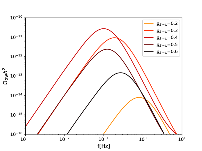
Figure 1: The predicted GW spectrum for various values of $g_{B-L}$ for $v_{2}=10$ TeV and $\lambda_{2}=0.002$.

Next, we focus on the VEV dependence of the resultant GW spectrum. We show in Fig. 2 the GW spectrum for various VEVs for the fixed values of $g_{B-L}=0.4$ and $\lambda_{2}=0.01$. We have found a very mild dependence for the amplitude but a strong dependence of the peak frequency. We have found an approximate relation of $f_{\mathrm{peak}}\propto v_{2}$. This can easily be understood, because $v_{2}$ is the only dimensionful parameter and scales the system as well as $T_{\star}$. Thus, we see $f_{\mathrm{peak}}\propto T_{\star}\propto v_{2}$ from Eq. (14).

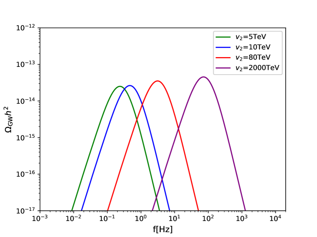
Figure 2: The predicted GW spectrum for various values of $v_{2}$ for $g_{B-L}=0.4$ and $\lambda_{2}=0.001$.

At last, we focus on the $\lambda_{2}$ dependence of the resultant GW spectrum. We show the GW spectrum for various $\lambda_{2}$ values for $g_{B-L}=0.4$ and $v_{2}=10$ TeV in Fig. 3. As $\lambda_{2}$ decreases, the peak frequency also decreases while the peak amplitude increases. We approximate relations such as $\Omega_{\mathrm{GW}}h^{2}(f_{\mathrm{peak}})\propto\lambda_{2}^{-1/4}$ and $f_{\mathrm{peak}}\propto\lambda_{2}$. We also find a lower bound on $\lambda_{2}$. As will be listed in Table 2, $\alpha$ is as large as $\mathcal{O}(1)$ for $\lambda_{2}\sim 10^{-4}$, which means that the energy density of background radiation and that of the latent heat is comparable. For $\lambda_{2}\ll 10^{-4}$, the latent heat becomes too large. Indeed, we find the effective equation of state parameter $w$ becomes smaller than $-1/3$ for such a too small $\lambda_{2}$ for $g_{B-L}=\mathcal{O}(0.1)$. In this case, the universe would inflate as in the old inflation model Sato:1980yn ; Guth:1980zm .

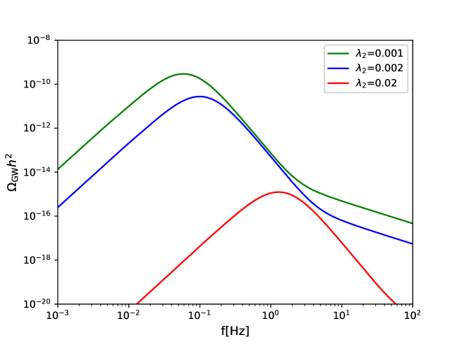
Figure 3: The predicted GW spectrum for various values of $\lambda_{2}$ for $g_{B-L}=0.4$ and $v_{2}=10$ TeV.

III.3 Predicted spectrum for benchmark points

We list our results for three benchmark points in Table 2.

Point	$g_{\mathrm{B-L}}$	$v_{2}$	$\lambda_{2}$	$\alpha$	$\beta/H_{\star}$	$T_{\star}$	$\varphi_{\mathrm{C}}/T_{\mathrm{C}}$
A	$0.44$	$4$ TeV	$1.5\times 10^{-4}$	$0.97$	$115.2$	$0.327$ TeV	$3.46$
B	$0.40$	$12$ TeV	$2.0\times 10^{-4}$	$0.32$	$304.5$	$1.032$ TeV	$3.64$
C	$0.46$	$3800$ TeV	$4.0\times 10^{-4}$	$0.96$	$115.4$	$328.7$ TeV	$3.30$

Table 2: Input and output parameters for several benchmark points are listed.

Here, the last quantity, $\varphi_{c}/T_{\mathrm{C}}$, is a typical measure of the strength of the first-order phase transition with the critical temperature $T_{\mathrm{C}}$ being the temperature when two minima are degenerate in the effective potential and $\varphi_{\mathrm{C}}$ being the value of the nontrivial minimum. In Fig. 4, we show predicted GW spectra for our benchmark points along with expected sensitivities of various future interferometer experiments. Green, blue, and red curves from left to right correspond to points A, B, and C, respectively. Black solid curves denote the expected sensitivities of each indicated experiments: LISA Sathyaprakash:2009xs , DECIGO and BBO Yagi:2011wg , aLIGO TheLIGOScientific:2014jea , and Cosmic Explore (CE) Evans:2016mbw . Curves are drawn by gwplotter Moore:2014lga . The sensitivities of DECIGO and BBO reach the results of the benchmark points A and B.

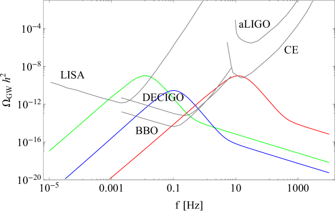
Figure 4: The predicted GW spectra for the benchmark points are shown. Green, blue and red curves from left to right correspond to points A, B, and C, respectively. The future experimental sensitivity curves of LISA Sathyaprakash:2009xs , DECIGO and BBO Yagi:2011wg , aLIGO TheLIGOScientific:2014jea , and Cosmic Explore (CE) Evans:2016mbw are also shown in black.

IV Summary

In this paper, we have calculated the spectrum of stochastic GW radiation generated by the cosmological phase transition of the minimal $U(1)_{B-L}$ model. We have found that a first-order phase transition strong enough to generate GWs with a detectable amplitude can be realized in the minimal $U(1)_{B-L}$ model with a single $B-L$ Higgs field, while an additional Higgs field has been thought to be necessary for such a strong first-order phase transition through previous studies. The Higgs potential of the minimal gauged $U(1)_{B-L}$ model is quite simple, and only three parameters are involved in our analysis. We clarify a dependence of the resultant GW spectrum on the three parameters: the peak amplitude is sensitive to the gauge coupling constant and the self-coupling constant, while the peak frequency is roughly proportional to the VEV of the $B-L$ Higgs field and the self-coupling constant. The $B-L$ phase transition at an energy scale far beyond the LHC reach can be observed through GWs in the future. We have also found, for a sensible value of the gauge coupling constant, the existence of a lower bound on the Higgs self-coupling constant $\lambda_{2}\gtrsim 10^{-4}$ in order not to realize an unwanted second inflation. We stress that, although our analysis has been done based on the $U(1)_{B-L}$ model, our results in this paper are general and applicable for any $U(1)$ gauge theory with a minimal Higgs sector, as long as Yukawa coupling effects on the effective Higgs potential are negligible.

References

- (1) R. N. Mohapatra and R. E. Marshak, Phys. Rev. Lett. 44, 1316 (1980) [Erratum-ibid. 44, 1643 (1980)].
- (2) R. E. Marshak and R. N. Mohapatra, Phys. Lett. B 91, 222 (1980).
- (3) T. Yanagida, Conf. Proc. C 7902131, 95 (1979).
- (4) M. Gell-Mann, P. Ramond, and R. Slansky, Conf. Proc. C 790927, 315 (1979).
- (5) R. N. Mohapatra and G. Senjanovic, Phys. Rev. Lett. 44, 912 (1980).
- (6) N. Okada and O. Seto, Phys. Rev. D 98, 063532 (2018).
- (7) V. Brdar, A. J. Helmboldt and J. Kubo, JCAP 1902, 021 (2019).
- (8) C. Grojean and G. Servant, Phys. Rev. D 75, 043507 (2007).
- (9) P. S. B. Dev and A. Mazumdar, Phys. Rev. D 93, 104001 (2016).
- (10) C. Balazs, A. Fowlie, A. Mazumdar and G. White, Phys. Rev. D 95, 043505 (2017).
- (11) R. Jinno and M. Takimoto, Phys. Rev. D 95, 015020 (2017).
- (12) C. Marzo, L. Marzola and V. Vaskonen, arXiv:1811.11169 [hep-ph].
- (13) S. Iso, N. Okada and Y. Orikasa, Phys. Lett. B 676, 81 (2009).
- (14) S. Iso, N. Okada and Y. Orikasa, Phys. Rev. D 80, 115007 (2009).
- (15) W. Chao, W. F. Cui, H. K. Guo and J. Shu, arXiv:1707.09759 [hep-ph].
- (16) W. Buchmuller, V. Domcke, K. Kamada and K. Schmitz, JCAP 1310, 003 (2013).
- (17) M. S. Turner and F. Wilczek, Phys. Rev. Lett. 65, 3080 (1990).
- (18) A. Kosowsky, M. S. Turner and R. Watkins, Phys. Rev. D 45, 4514 (1992).
- (19) A. Kosowsky, M. S. Turner and R. Watkins, Phys. Rev. Lett. 69, 2026 (1992).
- (20) M. S. Turner, E. J. Weinberg and L. M. Widrow, Phys. Rev. D 46, 2384 (1992).
- (21) A. Kosowsky and M. S. Turner, Phys. Rev. D 47, 4372 (1993).
- (22) M. Kamionkowski, A. Kosowsky and M. S. Turner, Phys. Rev. D 49, 2837 (1994).
- (23) A. Kosowsky, A. Mack and T. Kahniashvili, Phys. Rev. D 66, 024030 (2002).
- (24) A. D. Dolgov, D. Grasso and A. Nicolis, Phys. Rev. D 66, 103505 (2002).
- (25) G. Gogoberidze, T. Kahniashvili and A. Kosowsky, Phys. Rev. D 76, 083002 (2007).
- (26) C. Caprini, R. Durrer and G. Servant, JCAP 0912, 024 (2009).
- (27) M. Hindmarsh, S. J. Huber, K. Rummukainen and D. J. Weir, Phys. Rev. Lett. 112, 041301 (2014).
- (28) M. Hindmarsh, S. J. Huber, K. Rummukainen and D. J. Weir, Phys. Rev. D 92, 123009 (2015).
- (29) M. Hindmarsh, Phys. Rev. Lett. 120, 071301 (2018).
- (30) P. A. Seoane et al. [eLISA Collaboration], arXiv:1305.5720 [astro-ph.CO].
- (31) G. M. Harry, P. Fritschel, D. A. Shaddock, W. Folkner and E. S. Phinney, Class. Quant. Grav. 23, 4887 (2006); Erratum: [Class. Quant. Grav. 23, 7361 (2006)].
- (32) N. Seto, S. Kawamura and T. Nakamura, Phys. Rev. Lett. 87, 221103 (2001).
- (33) G. M. Harry [LIGO Scientific Collaboration], Class. Quant. Grav. 27, 084006 (2010).
- (34) C. Caprini and D. G. Figueroa, Class. Quant. Grav. 35, 163001 (2018).
- (35) A. Mazumdar and G. White, arXiv:1811.01948 [hep-ph].
- (36) S. J. Huber and T. Konstandin, JCAP 0809, 022 (2008).
- (37) R. Jinno and M. Takimoto, Phys. Rev. D 95, 024009 (2017).
- (38) J. R. Espinosa, T. Konstandin, J. M. No and G. Servant, JCAP 1006, 028 (2010).
- (39) C. Caprini et al., JCAP 1604, no. 04, 001 (2016).
- (40) J. Ellis, M. Lewicki and J. M. No, JCAP 1904, 003 (2019).
- (41) J. Ellis, M. Lewicki, J. M. No and V. Vaskonen, arXiv:1903.09642 [hep-ph].
- (42) P. Binetruy, A. Bohe, C. Caprini and J. F. Dufaux, JCAP 1206, 027 (2012).
- (43) R. Jinno, K. Nakayama and M. Takimoto, Phys. Rev. D 93, 045024 (2016).
- (44) M. Carena, A. Daleo, B. A. Dobrescu and T. M. P. Tait, Phys. Rev. D 70, 093009 (2004).
- (45) J. Heeck, Phys. Lett. B 739, 256 (2014).
- (46) N. Okada and S. Okada, Phys. Rev. D 93, 075003 (2016).
- (47) N. Okada and S. Okada, Phys. Rev. D 95, 035025 (2017).
- (48) N. Okada and O. Seto, Mod. Phys. Lett. A 33, 1850157 (2018).
- (49) S. Okada, Adv. High Energy Phys. 2018, 5340935 (2018).
- (50) C. L. Wainwright, Comput. Phys. Commun. 183, 2006 (2012).
- (51) See, e.g., M. Quiros, ICTP Ser. Theor. Phys. 15, p.187 (1999).
- (52) C. W. Chiang and E. Senaha, Phys. Lett. B 774, 489 (2017).
- (53) K. Sato, Mon. Not. Roy. Astron. Soc. 195 (1981) 467.
- (54) A. H. Guth, Phys. Rev. D 23, 347 (1981) [Adv. Ser. Astrophys. Cosmol. 3, 139 (1987)].
- (55) B. S. Sathyaprakash and B. F. Schutz, Living Rev. Rel. 12, 2 (2009).
- (56) K. Yagi and N. Seto, Phys. Rev. D 83, 044011 (2011); Erratum: [Phys. Rev. D 95, 109901 (2017)].
- (57) J. Aasi et al. [LIGO Scientific Collaboration], Class. Quant. Grav. 32, 074001 (2015).
- (58) B. P. Abbott et al. [LIGO Scientific Collaboration], Class. Quant. Grav. 34, 044001 (2017).
- (59) C. J. Moore, R. H. Cole and C. P. L. Berry, Class. Quant. Grav. 32, 015014 (2015).