Pressure Shifts in High–Precision Hydrogen Spectroscopy: I. Long–Range Atom–Atom and Atom–Molecule Interactions

Abstract

We study the theoretical foundations for the pressure shifts in high-precision atomic beam spectrosopy of hydrogen, with a particular emphasis on transitions involving higher excited $P$ states. In particular, the long-range interaction of an excited hydrogen atom in a $4P$ state with a ground-state and metastable hydrogen atom is studied, with a full resolution of the hyperfine structure. It is found that the full inclusion of the $4P_{1/2}$ and $4P_{3/2}$ manifolds becomes necessary in order to obtain reliable theoretical predictions, because the $1S$ ground state hyperfine frequency is commensurate with the $4P$ fine-structure splitting. An even more complex problem is encountered in the case of the $4P$–$2S$ interaction, where the inclusion of quasi-degenerate $4S$–$2P_{1/2}$ state becomes necessary in view of the dipole couplings induced by the van der Waals Hamiltonian. Matrices of dimension up to $40$ have to be treated despite all efforts to reduce the problem to irreducible submanifolds within the quasi-degenerate basis. We focus on the phenomenologically important second-order van der Waals shifts, proportional to $1/R^{6}$ where $R$ is the interatomic distance, and obtain results with full resolution of the hyperfine structure. The magnitude of van der Waals coefficients for hydrogen atom–atom collisions involving excited $P$ states is drastically enhanced due to energetic quasi-degeneracy; we find no such enhancement for atom-molecule collisions involving atomic $nP$ states, even if the complex molecular spectrum involving ro-vibrational levels requires a deeper analysis.

Keywords: Long-Range Interactions; Quasi-Degenerate States; Interatomic Interactions

1 Introduction

Investigations of van der Waals interactions involving excited states have attracted considerable attention [1, 2, 3, 4, 5, 6]. In the retarded regime, the phase of an oscillation of a virtual transition changes appreciably over the time it takes light to cover the interatomic distance. For excited reference states, one may obtain oscillatory long-range tails from the energetically lower, virtual states, which can give rise to interesting effects [7, 8, 9, 10, 11, 12]. We here analyze such interactions, with a particular emphasis on the evaluation of the pressure shift in the recent $2S$–$4P$ experiment carried out in Garching [13].

In the presence of quasi-degenerate states, the dominant contribution to the interaction is calculated by diagonalizing the Hamiltonian matrix in a basis of quasi-degenerate states, resulting in both first-order ($1/R^{3}$) and second-order ($1/R^{6}$) energy shifts [4]. Using today’s computer algebra [14], it is possible to set up the calculation with hyperfine resolution, i.e., to diagonalize the Hamiltonian matrix in a basis of states where all hyperfine levels, including their projections, are resolved, resulting in rather large matrices. In a quasi-degenerate basis, the energy separations are on the order of the Lamb shift energy with virtual transition wavelengths in the centimeter regime; hence, the retarded regime in this case is of no phenomenological relevance because of the small absolute magnitude of the energy shift in this range. In compensation, it is thus sufficient to treat the problem in the nonretardation approximation.

A significant motivation for an analysis of the fine-structure, and hyperfine-structure resolved levels, has been an ongoing experimental effort at a more high-precision measurement of the hydrogen $2S$–$4P$ transition in Garching [13], where the resolution of the hyperfine structure, together with the necessity to analyze collisional frequency shifts, calls for a much improved theoretical analysis of the van der Waals interaction, in comparison to previous approaches [15], which rely on nonrelativistic approximations.

As evident from the detailed analysis reported in the follow-up paper [16], excited-state interactions involving $4P$ states in contact with either ground-state $1S$ atoms or metastable $2S$ atoms are of prime importance [17, 18]. Phenomenologically, transitions to the $4P$ state have been much more relevant than, say, transitions to $P$ states with $n=6$ (see Ref. [19]), because of the much better accessible frequency range of the transition for lasers (see Refs. [20, 13]). Specifically, $2S$–$4P$ measurements have been carried out by a number of groups [20, 13], whereas $2S$–$6P$ transitions have not yet been measured to appreciable accuracy. The analysis is sufficiently complex that either system could not be analyzed without the use of computer algebra, due to the complex hyperfine structure state manifolds. It is thus of prime importance to generalize the treatment recently outlined in Ref. [19] to $4P$ states. Furthermore, because of the possible presence of hydrogen molecules in any atomic beam undergoing dissociation, it also becomes necessary to analyze the van der Waals coefficients for atom–molecule collisions, even if we can anticipate that the van der Waals coefficients will be drastically enhanced for collisions involving only atoms, because of the quasi-degeneracy of excited states, which are removed from each other only by the Lamb shift, fine- or hyperfine structure. Namely, the fine-structure and the hyperfine-structure splittings in the case of atom–atom interactions are very small compared to the energy differences between atomic and molecular quasi-degenerate levels, even if one consider possible excitations to ro-vibrational levels. For example, in the case of the $4P(H)$–$1S(H)$ interaction, the fine structure and the hyperfine structure splitting parameters are of the order of $2\times 10^{-7}\,E_{h}$ and $9\times 10^{-9}\,E_{h}$, respectively, where $E_{h}=27.211396\,$eV is the Hartree energy [21]. However, in the case of the $4P(H)$–$1S(H_{2})$ interaction, the atom-molecules degenerate states’ separation is in the order of $2\times 10^{-2}E_{h}$ and the ro-vibrational level splitting is at-most $\sim 5.5\times 10^{-5}E_{h}$. The oscillator strengths, in either cases, are of the same order of magnitude. As the respective energy differences appear in the denominator of the propagator denominators within perturbation theory, which determine the $C_{6}$ coefficients, we can anticipate that the so-called van der Waals $C_{6}$ coefficients are enhanced for atom-atom as compared to atom-molecule collisions. This is explained in greater detail in Sec. 5.

In order to understand the systems more deeply, we should consider the particular properties of the van der Waals Hamiltonian mediating the interaction. Let us refer to the atoms participating in the interaction as atoms $A$ and $B$. The static van der Waals Hamiltonian (without retardation), in the dipole approximation, involves the product of dipole operators of atoms $A$ and $B$. An $SP$ state, with atom $A$ in an $S$ state and atom $B$ in a $P$ state, can be coupled, by the van der Waals Hamiltonian, to a state with atom $A$ in a $P$ state and atom $B$ in an $S$ state. Or, a state with atoms $A$ and $B$ in $S$ states, can be coupled, by the van der Waals Hamiltonian, to a (possibly, quasi-degenerate) state with both atoms in $P$ states. This implies that the van der Waals interaction Hamiltonian needs to be diagonalized in the energetically degenerate subspaces composed of the $SS$, $SP$, $PS$ and $PP$ states of the two atoms [4]. However, because of the usual dipole selection rules, the $SS$ and $PP$ manifolds do not mix with the $SP$ states, and this reduces the size of the Hamiltonian matrices to be considered. The latter fact can be verified explicitly on the basis of adjacency graphs which demonstrate the irreducibility of the matrices in the basis of the $SP$ and $PS$ states [22]. Furthermore, interesting level crossings have been observed in the two-atom interaction despite the irreducibility of the matrices [4], and an explanation in terms of higher-order interactions (distance within the adjacency graphs) has been described in Ref. [22].

This paper is organized as follows. In Sec. 2, we outline the general formalism behind our considerations (Sec. 2), before treating the $4P$–$1S$ interactions (Sec. 3) and the $4P$–$2S$ interactions (Sec. 4). An interesting phenomenon is found in regard to the necessity of including both $4P_{1/2}$ as well as $4P_{3/2}$ states into the basis, and also $(4S;2P_{1/2})$ quasi-degenerate virtual states. We lay special emphasis onto the second-order van der Waals shifts incurred by the levels, averaged over the magnetic quantum numbers, as it is these numbers which are of highest phenomenological significance. Atom-molecule collisions are analyzed in Sec. 5, and finally, conclusions are drawn in Sec. 6. SI mksA units are used here, except in Sec. 4, where we switch to atomic units in order to keep formulas and mathematical expressions compact.

2 General Formalism

2.1 Interaction Hamiltonian

Let us briefly review the derivation of the van der Waals interaction and its application to excited states. Let $\vec{x}_{A}$ and $\vec{x}_{B}$ be the electron coordinates, and $\vec{R}_{A}$ and $\vec{R}_{B}$ be the coordinates of the protons. The total Coulomb interaction is

$$V_{\mathrm{C}}=\frac{e^{2}}{4\pi\epsilon_{0}}\left(\frac{1}{|\vec{R}_{A}-\vec{R}_{B}|}+\frac{1}{\left|\vec{x}_{A}-\vec{x}_{B}\right|}\right.\left.-\frac{1}{|\vec{x}_{A}-\vec{R}_{B}|}-\frac{1}{|\vec{x}_{B}-\vec{R}_{A}|}\right).\quad$$ (1)

One then uses the fact that the separation $|\vec{R}_{A}-\vec{R}_{B}|$ between the two nuclei (protons) is much larger than that between a given proton and its respective electron, that is, much larger than both $|\vec{r}_{A}|=|\vec{x}_{A}-\vec{R}_{A}|$ and $|\vec{r}_{B}|=|\vec{x}_{B}-\vec{R}_{B}|$. One then writes $\vec{x}_{A}-\vec{R}_{B}=\vec{r}_{A}+(\vec{R}_{A}-\vec{R}_{B})$ and $\vec{x}_{B}-\vec{R}_{A}=\vec{r}_{B}+(\vec{R}_{B}-\vec{R}_{A})$. Expanding in $\vec{r}_{A}$ and $\vec{r}_{B}$, one obtains [23, 24]

$$H_{\rm vdW} =\;\frac{e^{2}}{4\pi\epsilon_{0}}\,\frac{\vec{r}_{A}\cdot\vec{r}_{B}-3\,(\vec{r}_{A}\cdot\hat{R})\,(\vec{r}_{B}\cdot\hat{R})}{R^{3}}$$ (2)

$$=\;\frac{e^{2}}{4\pi\epsilon_{0}\,R^{3}}\,\left(\delta_{k\ell}-3\,\hat{R}_{k}\hat{R}_{\ell}\right)r_{Ak}\,r_{B\ell}=\;\frac{1}{4\pi\,\epsilon_{0}}\frac{\beta_{ij}\,d_{Ai}\,d_{Bj}}{R^{3}}\,,$$

where $\vec{R}=\vec{R}_{A}-\vec{R}_{B}$, $R=|\vec{R}|$ $\hat{R}=\vec{R}/R$ and $d_{A}=e\,r_{A}$ is an electric dipole moment for atom $A$ and $d_{B}$ is the same for atom $B$. We have introduced the tensor

$$\beta_{ik}=\delta_{ik}-3\frac{R_{i}\,R_{k}}{R^{2}}\,.$$ (3)

For definiteness, one chooses a quantization axis which enables one to resolve the magnetic projections in the hyperfine manifolds. This motivates the choice

$$\vec{R}=R\,\hat{e}_{z}\,,$$ (4)

which is henceforth applied universally to all systems studied in this paper.

In our analysis of $4P$–$1S$ interactions, a typical virtual transition involving quasi-degenerate states would involve atom $A$ in a $|4P_{J}\rangle$ state (with $J=\frac{1}{2}$ or $J=\frac{3}{2}$), and atom $B$ still in the $|1S\rangle$ state. This state is energetically degenerate with respect to a state where atom $A$ is in the $|1S\rangle$ state, and atom $B$ is in the $|4P_{J}\rangle$ state. Here, we further distinguish between absolute degeneracy (same unperturbed energy of the levels, even including the hyperfine interaction), and quasi-degeneracy, where levels are separated by the Lamb shift, or fine-structure interval. For the absolutely degenerate case, we incur first-order van der Waals shifts, linear in the van der Waals Hamiltonian $H_{\rm vdW}$, upon a rediagonalization of the total Hamiltonian.

An analogous situation is encountered for the $4P$–$2S$ interactions, with the additional complication that an additional degeneracy exists with respect to virtual $(4S;2P_{1/2})$ levels. Namely, the lower $2S$ state is removed from the $2P_{1/2}$ state only by the classic Lamb shift, and the $4S$ and $4P$ states are separated only by the $(n=4)$ fine-structure, or the $(n=4)$ Lamb shift. Hence, additional virtual states have to be taken into account in the discussion of the $4P$–$2S$ interaction.

2.2 Total Hamiltonian

In order to evaluate the $4P$–$nS$ long-range interaction, including hyperfine effects, and fine-structure effects, one needs to diagonalize the Hamiltonian

$$H=H_{{\mathrm{LS}},A}+H_{{\mathrm{LS}},B}+H_{{\mathrm{HFS}},A}+H_{{\mathrm{HFS}},B}+H_{{\mathrm{FS}},A}+H_{{\mathrm{FS}},B}+H_{{\mathrm{vdW}}}\,,$$ (5)

which sums over the atoms $A$ and $B$. Here, $H_{\rm LS}$ is the Lamb shift Hamiltonian, $H_{{\mathrm{FS}}}$ stands for the fine-structure splitting, while $H_{\rm HFS}$ describes hyperfine effects. We sum over the atoms $A$ and $B$. The Hamiltonians are given as follows,

$$H_{{\rm HFS},i}= \frac{\mu_{0}}{4\pi}\mu_{B}\mu_{N}\,g_{s}\,g_{p}\left[\frac{8\pi}{3}\vec{S}_{i}\cdot\vec{I}_{i}\,\delta^{(3)}\left(\vec{r}_{i}\right)\right.$$ (6a)

$$\left.+\frac{3(\vec{S}_{i}\cdot\vec{r}_{i})\,(\vec{I}_{i}\cdot\vec{r}_{i})-\vec{S}_{i}\cdot\vec{I}_{i}\;\left|\vec{r}_{i}\right|^{\,2}}{\left|\vec{r}_{i}\right|^{5}}+\frac{\vec{L}_{i}\cdot\vec{I}_{i}}{\left|\vec{r}_{i}\right|^{3}}\right]\,,$$

$$H_{{\rm LS},i}= \frac{4}{3}\frac{\hbar^{3}\,\alpha^{2}}{m_{e}^{2}\,c}\,\left(\frac{\hbar}{m_{e}c}\right)^{3}\ln\left(\alpha^{-2}\right)\delta^{3}\left(\vec{r}_{i}\right)\,,$$ (6b)

$$H_{{\rm FS},i}= -\frac{\vec{p}_{i}^{\,4}}{8m_{e}^{3}\,c^{2}}+\frac{\pi\,\hbar^{3}\,\alpha}{2\,m_{e}^{2}\,c}\,\delta^{(3)}(\vec{r}_{i})+\frac{g_{s}\,\hbar^{2}\,\alpha}{4\,m_{e}^{2}\,c\,\left|\vec{r}_{i}\right|^{3}}\vec{S}_{i}\cdot\vec{L}_{i}\,,$$ (6c)

$$H_{\rm vdW}= \frac{e^{2}}{4\pi\epsilon_{0}}\,\frac{x_{A}\,x_{B}+y_{A}\,y_{B}-2\,z_{A}\,z_{B}}{R^{3}}\,.$$ (6d)

The fine-structure constant is denoted as $\alpha$, $\mu_{0}$ is the vacuum permeability, and $m_{e}$ is the electron mass. We treat the system in the non-recoil approximation. The position and relative (with the respective nucleus) momentum operators are $\vec{r}_{i}$ and $\vec{p}_{i}$, while $\vec{L}_{i}$ is the orbital angular momentum operator. Also, $\vec{S}_{i}=\vec{\sigma}_{i}/2$ is the (dimensionless) spin operator for the electron $i$, where $\vec{\sigma}$ is the vector of Pauli spin matrices, and $\vec{I}_{i}$ is the spin operator for the nucleus of atom $i$ (proton $i$). According to Ref. [21], the protonic $g$ factors is $g_{p}\simeq$5.585\,695$$, $\mu_{B}\simeq$9.274\,010\text{\times}{10}^{-24}\text{\,}\mathrm{A}\mathrm{m}^{2}$$ is the Bohr magneton, while $\mu_{N}\simeq$5.050\,784\text{\times}{10}^{-27}\text{\,}\mathrm{A}\mathrm{m}^{2}$$ is the nuclear magneton. In order to simplify the expressions, we use the approximation $g_{s}=2$ in the following calculations.

For the $4P$–$1S$ system, our convention is that the zero of the energy scale is the sum of the Dirac energies of the $1S$ and $4P_{1/2}$ states (in the case of the $4P$–$1S$ interaction), and to the sum of the $2S$ and $4P_{1/2}$ states (in the case of the $4P$–$2S$ interaction). The zero point of the energy excludes both Lamb shift as well as hyperfine effects. On the basis of the Welton approximation, we add the Lamb shift energy to the $S$ states, adjusted for the $S$–$P$ energy difference to match the experimentally observed splitting, but leave the $P$ states untouched by Lamb shift effects. Hence, strictly speaking, our definition of the zero point of the energy would correspond to the hyperfine centroid of the $|(4P_{1/2})_{A}(1S)_{B}\rangle$ states (see Sec. 3), and to the hyperfine centroid of the $|(4P_{1/2})_{A}(2P_{1/2})_{B}\rangle$ states (see Sec. 4). The fine-structure energy is being added to the $4P_{3/2}$ states. For the calculation of the van der Waals interaction energies, the precise definition of the zero point is not of relevance because only the energy difference in the quasi-degenerate basis matters.

The expression for $H_{\rm LS}$ in Eq. (6b) follows the Welton approximation [25]; for the calculation of energy shifts, we shall replace

$$\langle nS_{1/2}|H_{LS}|nS_{1/2}\rangle= \;\frac{4\alpha}{3\pi}\,\frac{\alpha^{4}}{n^{3}}\,m_{e}\,c^{2}\,\ln(\alpha^{-2})\to{\mathcal{L}}_{n}\,,$$ (6ga)

$$\langle nP_{1/2}|H_{LS}|nP_{1/2}\rangle= \;0\,,$$ (6gb)

where ${\mathcal{L}}_{n}$ is the $nS$ Lamb shift, which we understand as the $nS_{1/2}$–$nP_{1/2}$ energy difference. These replacements are consistent with our definition of the zero of the energy scale, as discussed above. Throughout this paper, we perform final numerical evaluations in the non-recoil approximation, which corresponds to an infinite mass of the proton, i.e., we set the reduced mass of the electron in hydrogen atom equal to the electron mass, and ignore the different reduced-mass dependence for the fine-structure and the hyperfine-structure terms in the Hamiltonian. Values for physical constants are taken from Ref. [21].

2.3 Explicit Construction of the States

Even if the relevant procedure has recently been described in some detail in Sec. IIB of Ref. [4], and in Sec. I of Ref. [19], we here recall how to construct the atomic states for the hyperfine-resolved $4P_{1/2}$–$1S$ interaction. The relevant quantum numbers are

$$1S_{1/2}(F=0):n=1,\,\ell=0,\,J=\frac{1}{2},\,F=0\,,$$ (6gha)

$$1S_{1/2}(F=1):n=1,\,\ell=0,\,J=\frac{1}{2},\,F=1\,,$$ (6ghb)

$$4P_{1/2}(F=0):n=4,\,\ell=1,\,J=\frac{1}{2},\,F=0\,,$$ (6ghc)

$$4P_{1/2}(F=1):n=4,\,\ell=1,\,J=\frac{1}{2},\,F=1\,.$$ (6ghd)

Here, $n$ is the principal quantum number, while $\ell$, $J$, and $F$ are the electronic orbital angular momentum, the total (orbital$+$spin) electronic angular momentum and the total (electronic$+$protonic) atomic angular momentum, respectively. Here and in the following, we denote by $F$ and ${\mathfrak{F}}_{z}$ the total angular momenta (orbital$+$electron spin$+$nuclear spin) of either atom $A$ or $B$, which can be specified for either atom by adding the respective subscript. By contrast, ${\mathfrak{F}}$ is their vector sum $\vec{\mathfrak{F}}=\vec{F}_{A}+\vec{F}_{B}$, so that, in particular, ${\mathfrak{F}}_{z}=F_{z,A}+F_{z,B}$.

We denote by $\left|\pm\right\rangle_{e}$ the electron spin state, while $|n,\ell,m\rangle_{e}$ denotes the Schrödinger eigenstate (without spin). We need to add the nuclear (proton) spin $|\pm\rangle_{p}$ to the electron angular momentum. For illustration, we indicate the explicit form of the hyperfine singlet $4P_{1/2}$ state,

$$\quad\left|n=4,\ell=1,J=\frac{1}{2},F=0,F_{z}=0\right\rangle=\frac{1}{\sqrt{3}}\left|+\right\rangle_{p}\left|+\right\rangle_{e}\left|4,1,-1\right\rangle_{e}$$

$$\quad\quad-\frac{1}{\sqrt{6}}\left|+\right\rangle_{p}\left|-\right\rangle_{e}\left|4,1,0\right\rangle_{e}+\frac{1}{\sqrt{3}}\left|-\right\rangle_{p}\left|-\right\rangle_{e}\left|4,1,1\right\rangle_{e}-\frac{1}{\sqrt{6}}\left|-\right\rangle_{p}\left|+\right\rangle_{e}\left|4,1,0\right\rangle_{e}\,,$$ (6ghi)

while the hyperfine triplet states in the $4P_{1/2}$ manifold read as follows,

$$\quad\left|n=4,\ell=1,J=\frac{1}{2},F=1,F_{z}=0\right\rangle=-\frac{1}{\sqrt{3}}\left|+\right\rangle_{p}\left|+\right\rangle_{e}\left|4,1,-1\right\rangle_{e}$$

$$\quad\;\;+\frac{1}{\sqrt{6}}\left|+\right\rangle_{p}\left|-\right\rangle_{e}\left|4,1,0\right\rangle_{e}+\frac{1}{\sqrt{3}}\left|-\right\rangle_{p}\left|-\right\rangle_{e}\left|4,1,1\right\rangle_{e}-\frac{1}{\sqrt{6}}\left|-\right\rangle_{p}\left|+\right\rangle_{e}\left|4,1,0\right\rangle_{e}\,,$$ (6ghj)

and

$$\quad\left|n=4,\ell=1,J=\frac{1}{2},F=1,F_{z}=\pm 1\right\rangle$$

$$\quad\quad=\mp\frac{1}{\sqrt{3}}\left|\pm\right\rangle_{p}\left\{\left|\pm\right\rangle_{e}\left|4,1,0\right\rangle_{e}\right.-\sqrt{2}\left.\left|\mp\right\rangle_{e}\,\left|4,1,\pm 1\right\rangle_{e}\right\}.$$ (6ghk)

Just like in Ref. [19], we shall use the notation $|n,\ell,J,F,F_{z}\rangle$ for the thusly obtained states, using the vector coupling coefficients, with principal quantum number $n$, orbital quantum number $\ell$, total electron angular quantum number $J$, total angular quantum number $F$ (electron$+$nucleus), and total magnetic projection quantum number $F_{z}$.

Up to the hyperfine-fine-structure mixing term, which is discussed in Eq. (6ghyajav), these states are eigenstates of the unperturbed Hamiltonian

$$H_{0}=H_{{\mathrm{LS}},A}+H_{{\mathrm{LS}},B}+H_{{\mathrm{FS}},A}+H_{{\mathrm{FS}},B}+H_{{\mathrm{HFS}},A}+H_{{\mathrm{HFS}},B}\,.$$ (6ghl)

Based on the explicit representations of the relevant, hyperfine-resolved atomic states, one can easily develop a computer symbolic program, using computer algebra [14], which determines the matrix elements of the total Hamiltonian (5) among all states within the hyperfine-resolved basis. A different approach to the calculation of the matrix elements, especially useful for the evaluation of matrix elements of the van der Waals Hamiltonian, is based on the Wigner-Eckhart theorem, and will be discussed in the following.

2.4 Wigner–Eckhart Theorem

It is very important and instructive to recall that the evaluation of the matrix elements of the long-range interaction Hamiltonian (2), in the hyperfine-resolved basis, can also be accomplished with the help of the Wigner–Eckhart theorem, as an alternative to the explicit construction of states outlined in Sec. 2.3. To this end, one writes the van der Waals Hamiltonian, given in Eq. (2), as

$$H_{\rm vdW}=-\frac{e^{2}}{4\pi\epsilon_{0}}\frac{x_{A,-1}\,x_{B,+1}+x_{A,+1}\,x_{B,-1}+2x_{A,0}\,x_{B,0}}{R^{3}},$$ (6ghm)

where the coordinates, in the spherical basis, are

$$x_{A,+1}=-\frac{1}{\sqrt{2}}\,(x_{A}+{\mathrm{i}}\,y_{A})\,,\quad x_{A,-1}=\frac{1}{\sqrt{2}}\,(x_{A}-{\mathrm{i}}\,y_{A})\,,\quad x_{A,0}=z_{A}\,,$$ (6ghn)

and same for atom $B$.

The unperturbed states are of the form $|n,\ell,J,F,m_{F},(S),(I)\rangle$ where we have previously defined the states as $|n,\ell,J,F,m_{F}\rangle$ with all quantum numbers being explained previously. The “hidden” quantum numbers are the electron spin $S$, and the nuclear spin $I$. For hydrogen, these attain the values $S=I=\frac{1}{2}$ and are the same for all hydrogen states being discussed here. Still, the quantum numbers $S$ and $I$ need to be taken into account in the vector recoupling which will be described in the following. First, one eliminates the magnetic quantum numbers $m_{F}$ and $m^{\prime}_{F}$ by the Wigner–Eckhart theorem,

$$\langle n^{\prime},\ell^{\prime},J^{\prime},F^{\prime},m^{\prime}_{F},(S),(I)|\,T^{1}_{q}\,|n,\ell,J,F,m_{F},(S),(I)\rangle=(-1)^{F^{\prime}-m_{F}^{\prime}}\left(\begin{array}[]{ccc}F^{\prime}&1&F\\ -m_{F}^{\prime}&q&m_{F}\end{array}\right)$$ (6ghq)

$$\times\langle n^{\prime},\ell^{\prime},J^{\prime},F^{\prime},(S),(I)||\,\vec{T}(1)\,||n,\ell,J,F,(S),(I)\rangle\,,$$ (6ghr)

where $T^{1}_{q=-1,0,1}$ are the elements of a tensor, the specialization to the case $k=1$ of a tensor $T^{k}_{q}$ of rank $k$, and $\langle n^{\prime},\ell^{\prime},J^{\prime},F^{\prime},(S),(I)||\,\vec{T}(1)\,||n,\ell,J,F,(S),(I)\rangle$ is the reduced matrix element. The nuclear and electronic degrees of freedom can be separated using a 6$j$ symbol (vector recoupling coefficient) as described in Refs. [26, 27],

$$\langle n^{\prime},\ell^{\prime},J^{\prime},F^{\prime},(S),(I)||\,{\vec{T}}(1)\,||n,\ell,J,F,(S),(I)\rangle=(-1)^{J^{\prime}+I+F+1}\,\sqrt{(2F+1)(2F^{\prime}+1)}$$

$$\times\left\{\begin{array}[]{ccc}J^{\prime}&F^{\prime}&I\\ F&J&1\end{array}\right\}\langle n^{\prime},\ell^{\prime},J^{\prime},(S)||\,{\vec{T}}(1)\,||n,\ell,J,(S)\rangle\,.$$ (6ghu)

Another vector recoupling coefficient is needed in order to separate the orbital angular momentum of the electron from the electron spin,

$$\langle n^{\prime},\ell^{\prime},J^{\prime},(S)||\,{\vec{T}}(1)\,||n,\ell,J,(S)\rangle =(-1)^{L^{\prime}+S+J+1}\,\sqrt{(2J+1)(2J^{\prime}+1)}$$ (6ghx)

$$\times\left\{\begin{array}[]{ccc}L^{\prime}&J^{\prime}&S\\ J&L&1\end{array}\right\}\langle n^{\prime},\ell^{\prime}||\,{\vec{T}}(1)\,||n,\ell\rangle\,.$$

The following results for the reduced matrix elements,

$$\langle n^{\prime}=1,\ell^{\prime}=0||\,{\vec{r}}\,||n=4,\ell=1\rangle= \;-3\,\frac{2^{11}}{5^{6}}\,\sqrt{\frac{3}{5}}\,a_{0}\,,$$ (6ghya)

$$\langle n^{\prime}=4,\ell^{\prime}=1||\,{\vec{r}}\,||n=1,\ell=0\rangle= \;3\,\frac{2^{11}}{5^{6}}\,\sqrt{\frac{3}{5}}\,a_{0}\,,$$ (6ghyb)

$$\langle n^{\prime}=2,\ell^{\prime}=0||\,{\vec{r}}\,||n=4,\ell=1\rangle= \;-\frac{2^{9}}{3^{6}}\,\sqrt{\frac{10}{3}}\,a_{0}\,,$$ (6ghyc)

$$\langle n^{\prime}=4,\ell^{\prime}=1||\,{\vec{r}}\,||n=2,\ell=0\rangle= \;\frac{2^{9}}{3^{6}}\,\sqrt{\frac{10}{3}}\,a_{0}\,,$$ (6ghyd)

$$\langle n^{\prime}=2,\ell^{\prime}=0||\,{\vec{r}}\,||n=2,\ell=1\rangle= \;3\,\sqrt{3}\,a_{0}\,,$$ (6ghye)

$$\langle n^{\prime}=2,\ell^{\prime}=1||\,{\vec{r}}\,||n=2,\ell=0\rangle= \;-3\,\sqrt{3}\,a_{0}\,,$$ (6ghyf)

for the rank one tensor $\vec{r}=\vec{T}(1)$, cover all states relevant to the current investigation. In order to evaluate the elements, one expresses them, after the application of the Wigner–Eckhart theorem, in terms of radial integrals involving the standard hydrogenic bound-state wave functions [28, 29].

3 $\bm{4P}$–$\bm{1S}$ Interaction

Table 1: Multiplicities in the $4P_{1/2}$–$4P_{3/2}$–$1S$ system. One might wonder why ${\mathfrak{F}}_{z}=\pm 3$ is possible for $F=2$. The answer is that $F=2$ here refers to the total angular momentum (electron orbital plus electron spin plus nuclear spin) of one of the atoms, while ${\mathfrak{F}}_{z}=\pm 3$ refers to the angular momentum projection of the sum of the total angular momenta of both electrons i.e., ${\mathfrak{F}}_{z}=F_{z,A}+F_{z,B}$.

	${\mathfrak{F}}_{z}=0$	${\mathfrak{F}}_{z}=\pm 1$	${\mathfrak{F}}_{z}=\pm 2$	${\mathfrak{F}}_{z}=\pm 3$
$(J=\frac{3}{2},F=2)$	8	8	6	2
$(J=\frac{3}{2},F=1)$	8	6	2	0
$(J=\frac{3}{2})$	16	14	8	2
$(J=\frac{1}{2},F=1)$	8	6	2	0
$(J=\frac{1}{2},F=0)$	4	2	0	0
$(J=1/2)$	12	8	2	0
$(J=\frac{1}{2})+(J=\frac{3}{2})$	28	22	10	2

3.1 Selection of the States

The task is to diagonalize the Hamiltonian given in Eq. (5),

$$H=H_{{\mathrm{LS}},A}+H_{{\mathrm{LS}},B}+H_{{\mathrm{HFS}},A}+H_{{\mathrm{HFS}},B}+H_{{\mathrm{FS}},A}+H_{{\mathrm{FS}},B}+H_{{\mathrm{vdW}}}\,,$$ (6ghyz)

in a quasi-degenerate basis, for two atoms, the first being in a $4P$ state, the second being in a substate of the $1S$ hyperfine manifold. Retardation does not need to be considered. According to Refs. [30, 31], the $4P$ fine-structure frequency $\nu_{\rm FS}=\nu(4P_{3/2}-4P_{1/2})$,

$$\nu_{\rm FS}\approx 1\,371\,{\rm MHz}\,,$$ (6ghyaa)

approximately coincides with the $1S$ hyperfine-structure frequency

$$\nu_{\rm HFS}\approx 1\,420\,{\rm MHz}\,,$$ (6ghyab)

which is the $21\,{\rm cm}$ line. Hence, in order to be self-consistent, we need to include both the $4P_{1/2}$ as well as the $4P_{3/2}$ states into our hyperfine-resolved basis.

We select the $(4P)_{A}(1S)_{B}$ and $(1S)_{A}(4P)_{B}$ states, with all hyperfine levels resolved, from the respective manifolds, and obtain the following total multiplicities when all $4P_{1/2}$ and $4P_{3/2}$ states are added into the basis (see also Table 1)

$$\eqalign{g({\mathfrak{F}}_{z}=\pm 3)=\;2\,,\qquad g({\mathfrak{F}}_{z}=\pm 2)=\;10\,,\cr g({\mathfrak{F}}_{z}=\pm 1)=\;22\,,\qquad g({\mathfrak{F}}_{z}=0)=\;28\,.}$$ (6ghyae)

The multiplicities are the sums of the multiplicities in the $4P_{3/2}$–$1S$ system,

$$\eqalign{g(J=\frac{3}{2},{\mathfrak{F}}_{z}=\pm 3)=\;2\,,\qquad g(J=\frac{3}{2},{\mathfrak{F}}_{z}=\pm 2)=\;8\,,\cr g(J=\frac{3}{2},{\mathfrak{F}}_{z}=\pm 1)=\;14\,,\qquad g(J=\frac{3}{2},{\mathfrak{F}}_{z}=0)=\;16\,,}$$ (6ghyah)

and in the $4P_{1/2}$–$1S$ system,

$$g(J=\frac{1}{2},{\mathfrak{F}}_{z}=\pm 2)=\;2\,,\quad g(J=\frac{1}{2},{\mathfrak{F}}_{z}=\pm 1)=\;8\,,\quad g(J=\frac{1}{2},{\mathfrak{F}}_{z}=0)=\;12\,.$$ (6ghyai)

We work with the full $J=\frac{1}{2}$ and $J=\frac{3}{2}$ manifolds throughout our investigation.

3.2 Matrix Elements of the Total Hamiltonian

Matrix elements of the total Hamiltonian (5) now have to be computed in the space spanned by the two-atom states, which are given in Eqs. (2.3)–(2.3) (for the $4P_{1/2}$ states), as well as the $4P_{3/2}$ states. These elements may either be determined by a computer symbolic program [14] or using the Wigner-Eckart procedure described in Sec. 2.4. It is useful to define the parameters

$${\mathcal{H}} \equiv\frac{\alpha^{4}}{18}\,g_{p}\,\frac{m_{e}}{m_{p}}\,m_{e}\,c^{2}=h\,59.21498\,{\rm MHz}\,,$$ (6ghyaja)

$${\mathcal{L}}_{2} \equiv h\,1057.845(9)\,{\rm MHz}\,,$$ (6ghyajb)

$${\mathcal{L}}_{4} \equiv h\times\frac{1}{8}\,\times 1057.845(9)\,{\rm MHz}\,,$$ (6ghyajc)

$${\mathcal{F}} \equiv\frac{\alpha^{4}\,m_{e}\,c^{2}}{256}=h\,1368.660\,{\rm MHz}\,,$$ (6ghyajd)

$${\mathcal{V}}(\rho) \equiv 3\,\frac{e^{2}}{4\pi\epsilon_{0}}\,\frac{a_{0}^{2}}{R^{3}}=\frac{3\,E_{h}}{\rho^{3}}\,,$$ (6ghyaje)

$${\mathcal{W}}(\rho) \equiv\frac{3\times 2^{22}}{5^{13}}\,\frac{e^{2}}{4\pi\epsilon_{0}}\,\frac{a_{0}^{2}}{R^{3}}=\frac{3\times 2^{22}}{5^{13}}\,\frac{E_{h}}{\rho^{3}}\,,$$ (6ghyajf)

where $R=a_{0}\rho$, and $a_{0}$ is the Bohr radius, ${\mathcal{L}}_{4}$ is the $4S-4P_{1/2}$ Lamb shift, and $E_{h}=\alpha^{2}m_{e}c^{2}$ is the Hartree energy. Our symbol ${\mathcal{H}}$ is equivalent to one-third of the hyperfine splitting of the $2S$ state [32], while ${\mathcal{L}}_{2}$ is the $2S$–$2P_{1/2}$ Lamb shift [33]. The interaction energy ${\mathcal{V}}(\rho)$ depends on the interatomic separation $R$, viz., $\rho$. We have used the identity

$$\frac{e^{2}}{4\pi\epsilon_{0}}\,\frac{a_{0}^{2}}{R^{3}} =\;\frac{4\pi\alpha\epsilon_{0}\hbar c}{4\pi\epsilon_{0}}\,\frac{\alpha m_{e}c}{\hbar}\,\frac{1}{\rho^{3}}=\;\frac{\alpha\hbar c\,\alpha m_{e}c}{\hbar}\,\frac{1}{\rho^{3}}=\frac{\alpha^{2}m_{e}c^{2}}{\rho^{3}}=\frac{E_{h}}{\rho^{3}}\,.$$ (6ghyajak)

The natural scale for the constants ${\mathcal{H}}$ and ${\mathcal{L}}$ is an energy of order $\alpha^{3}\,E_{h}$. Hence, we write

$${\mathcal{H}}=\;\alpha^{3}\,E_{h}\,C_{{\mathcal{H}}}\,,\qquad{\mathcal{L}}_{n}=\;\alpha^{3}\,E_{h}\,C_{{\mathcal{L}},n}\,,\qquad{\mathcal{F}}= \;\alpha^{3}\,E_{h}\,C_{{\mathcal{F}}}\,,$$ (6ghyajal)

where we set $C_{{\mathcal{H}}}=g_{p}/18\alpha\times(m_{e}/m_{p})=0.0231596$, $C_{{\mathcal{F}}}=1/256\alpha=0.5352969$ and $C_{{\mathcal{L}},4}=C_{{\mathcal{L}},2}/8=0.0517167$. Then, we can write for typical expressions of second-order energy shifts,

$$\frac{{\mathcal{V}}^{2}(\rho)}{T_{1}{\mathcal{H}}+T_{2}{\mathcal{L}}_{n}+T_{3}{\mathcal{F}}}=\frac{9}{T_{1}\,C_{{\mathcal{H}}}+T_{2}\,C_{{\mathcal{L}},n}+T_{3}C_{{\mathcal{F}}}}\,\,\frac{E_{h}}{\alpha^{3}\,\rho^{6}}\,,$$ (6ghyajam)

where $T_{1}$, $T_{2}$ and $T_{3}$ typically are rational fractions, to be determined by separate calculations.

A particularly interesting feature is that the hyperfine Hamiltonian actually is not diagonal in the space of the $4P_{1/2}$ and $4P_{3/2}$ states. Rather, one has a mixing among the $F=1$ states of the $4P_{1/2}$ and $4P_{3/2}$ manifolds, with the mixing matrix element being given by (see Ref. [34] for an outline of the calculation)

$$\langle 4P_{3/2}^{F=1}(F_{z})|H_{\rm HFS}|4P_{1/2}^{F=1}(F_{z})\rangle=X\,.$$ (6ghyajan)

We restrict the discussion here to one atom only, say, atom $A$, omitting the subscript on $H_{\rm HFS}\equiv H_{{\rm HFS},A}$. For the two states to be coupled, the magnetic projection $F_{z}$ has to be the same, though. Otherwise, the matrix element vanishes. Thus, in the basis of states

$$|a\rangle=\;|4P_{1/2}^{F=1}F_{z}=1)\rangle=|4,1,\frac{1}{2},1,1\rangle\,,\quad|b\rangle=\;|4P_{1/2}^{F=1}(F_{z}=0)\rangle=|4,1,\frac{1}{2},1,0\rangle\,,$$ (6ghyajao)

$$|c\rangle=\;|4P_{1/2}^{F=1}F_{z}=-1)\rangle=|4,1,\frac{1}{2},1,-1\rangle\,,\quad|d\rangle=\;|4P_{3/2}^{F=1}(F_{z}=1)\rangle=|4,1,\frac{3}{2},1,1\rangle\,,$$

$$|e\rangle=\;|4P_{3/2}^{F=1}(F_{z}=0)\rangle=|4,1,\frac{3}{2},1,0\rangle\,,\quad|f\rangle=\;|4P_{3/2}^{F=1}(F_{z}=-1)\rangle=|4,1,\frac{3}{2},1,-1\rangle\,,$$

the matrix of the Hamiltonian $H_{\rm HFS}+H_{\rm FS}$ is evaluated as

$$H_{\rm HFS+FS}=\left(\begin{array}[]{cccccc}D&0&0&X&0&0\\ 0&D&0&0&X&0\\ 0&0&D&0&0&X\\ X&0&0&-D+{\mathcal{F}}&0&0\\ 0&X&0&0&-D+{\mathcal{F}}&0\\ 0&0&X&0&0&-D+{\mathcal{F}}\\ \end{array}\right),$$ (6ghyajav)

where

$$D=g_{p}\frac{\alpha^{4}m_{e}^{2}c^{2}}{576\,m_{p}}\,,\qquad X=-g_{p}\frac{\alpha^{4}m_{e}^{2}c^{2}}{1152\,\sqrt{2}\,m_{p}}\,.$$ (6ghyajaw)

Here, $g_{p}$ is the proton $g$ factor, while $D$ is a diagonal matrix element, and $X$ is the off-diagonal element given above.

The $6\times 6$ Hamiltonian matrix (6ghyajav) can be decomposed into three identical submatrices corresponding to $F_{z}=-1,0$ and $+1$. Each submatrix is of dimension two, e.g., the one spanned by $|a\rangle$ and $|d\rangle$. The Hamiltonian matrix is

$$H^{F_{z}=1}_{\rm HFS+FS}=\left(\begin{array}[]{cc}D&X\\ X&-D+{\mathcal{F}}\\ \end{array}\right).$$ (6ghyajaz)

The eigenvalues of $H^{F_{z}=1}_{\rm HFS+FS}$ are given by

$$\mathcal{E}_{+}=-D+{\mathcal{F}}+\frac{X^{2}}{{\mathcal{F}}-2D}+\Or(X^{4})\,,$$ (6ghyajbaa)

$$\mathcal{E}_{-}=D-\frac{X^{2}}{{\mathcal{F}}-2D}+\Or(X^{4}).$$ (6ghyajbab)

The second-order shift in the eigenvalues, $\Delta=X^{2}/({\mathcal{F}}-2D)$, is numerically equal to $$4.7659\text{\times}{10}^{-14}$E_{h}$, where $E_{h}=\alpha^{2}m_{e}c^{2}$ is the Hartree energy. For simplicity, we thus define the parameter

$$\Delta=$4.7659\text{\times}{10}^{-14}$\,,\qquad\frac{\Delta\cdot E_{h}}{h}=$313.58\text{\,}\mathrm{Hz}$\,.$$ (6ghyajbabb)

The normalized eigenvectors of $H^{F_{z}=1}_{\rm HFS-FS}$ are

$$|\varphi_{+}\rangle=\frac{1}{\sqrt{\alpha_{-}^{2}+1}}\left(\alpha_{-}\,|a\rangle+|d\rangle\right)\,,$$ (6ghyajbabca)

$$|\varphi_{-}\rangle=\frac{1}{\sqrt{\alpha_{+}^{2}+1}}\left(\alpha_{+}\,|a\rangle+|d\rangle\right)\,,$$ (6ghyajbabcb)

where the coefficients $\alpha_{\pm}$ are given by

$$\alpha_{\pm}=\frac{2D-{\mathcal{F}}\pm\sqrt{4(D^{2}-D{\mathcal{F}}+X^{2})+{\mathcal{F}}^{2}}}{2X}\,.$$ (6ghyajbabcbd)

Examples of expectation values of the hyperfine $H_{\mathrm{HFS}}$ and Lamb shift $H_{\mathrm{LS}}$ Hamiltonians (for states of both atoms $A$ and $B$) are

$$F_{z}\langle n,\ell,J,F,F_{z}|H_{\mathrm{LS}}|n,\ell,J,F,F_{z}\rangle=\;\mathcal{L}_{n}\,\delta_{\ell 0},$$ (6ghyajbabcbea)

$$\langle 1,0,\frac{1}{2},1,F_{z}|H_{\mathrm{HFS}}|1,0,\frac{1}{2},1,F_{z}\rangle=\;6\,\mathcal{H}\,,$$ (6ghyajbabcbeb)

$$\langle 1,0,\frac{1}{2},0,0|H_{\mathrm{HFS}}|1,0,\frac{1}{2},0,0\rangle=\;-18\,\mathcal{H}\,,$$ (6ghyajbabcbec)

$$\langle 4,1,\frac{1}{2},1,F_{z}|H_{\mathrm{HFS}}|4,1,\frac{1}{2},1,F_{z}\rangle=\;\frac{1}{32}\,\mathcal{H}\,,$$ (6ghyajbabcbed)

$$\langle 4,1,\frac{1}{2},0,0|H_{\mathrm{HFS}}|4,1,\frac{1}{2},0,0\rangle=\;-\frac{3}{32}\,\mathcal{H}\,.$$ (6ghyajbabcbee)

$$\langle 4,1,\frac{3}{2},2,F_{z}|H_{\mathrm{HFS}}|4,1,\frac{3}{2},2,F_{z}\rangle=\;\frac{3}{160}\,\mathcal{H}\,,$$ (6ghyajbabcbef)

$$\langle 4,1,\frac{3}{2},1,F_{z}|H_{\mathrm{HFS}}|4,1,\frac{3}{2},1,F_{z}\rangle=\;-\frac{1}{32}\,\mathcal{H}\,.$$ (6ghyajbabcbeg)

The hyperfine splitting energy between $4P_{1/2}(F=1)$ and $4P_{1/2}(F=0)$ states thus amounts to $\mathcal{H}/8$, while between $4P_{3/2}(F=2)$ and $4P_{3/2}(F=1)$ states, it is $\mathcal{H}/20$. The $1S$-state hyperfine splitting is $24\mathcal{H}$. For the product state of atoms $A$ and $B$, we shall use the notation

$$|(n_{A},\ell_{A},J_{A},F_{A},F_{z,A})_{A}\,(n_{B},\ell_{B},J_{B},F_{B},F_{z,B})_{B}\,\rangle\,,$$ (6ghyajbabcbebf)

which summarizes the quantum numbers of both atoms.

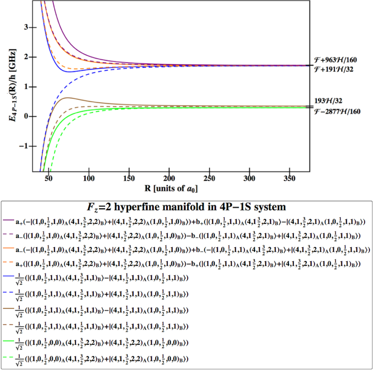
Figure 1: Evolution of the energy levels as a function of interatomic distance. The vertical axis is the energy divided by the Planck constant and given in units of $10^{9}\,{\rm Hz}$ (GHz). The interatomic separation in the horizontal axis is in units of Bohr’s radius. At large separation, there are four energy levels, which match the number of unperturbed energy values of matrix $H_{F_{z}=2}$. As the interatomic distance decreases, the energy levels repel each other and are visually discernible. The coefficients $a_{\pm}$ and $b_{\pm}$ are given by Eq. (6ghyajbabcbebmcxcycz).

3.3 Manifold ${{\mathfrak{F}}_{z}=3}$

States can be classified according to the quantum number ${\mathfrak{F}}_{z}=F_{z,A}+F_{z,B}$, because the $z$ component of the total angular momentum commutes [4] with the total Hamiltonian given in Eq. (5). Within the $4P_{1/2}$–$4P_{3/2}$–${1S}_{1/2}$ system, the states in the manifold ${\mathfrak{F}}_{z}=3$ are given as follows,

$$|\phi_{1}\rangle=\;|(1,0,\frac{1}{2},1,1)_{A}\,(4,1,\frac{3}{2},2,2)_{B}\rangle\,,\quad|\phi_{2}\rangle= \;|(4,1,\frac{3}{2},2,2)_{A}\,(1,0,\frac{1}{2},1,1)_{B}\rangle.$$ (6ghyajbabcbebg)

In full analogy to the $1S$–$6P$ system analyzed in Ref. [19], we have ordered the basis vectors in ascending order of the quantum numbers, starting from the last member in the list. The Hamiltonian matrix evaluates to

$$H_{{\mathfrak{F}}_{z}=3}=\left(\begin{array}[]{cc}\frac{963}{160}\,{{\mathcal{H}}}{}+{\mathcal{F}}&\frac{3\times 2^{22}}{5^{13}}{{\mathcal{V}}}{}(\rho)\\[8.61108pt] \frac{3\times 2^{22}}{5^{13}}{{\mathcal{V}}}{}(\rho)&\frac{963}{160}\,{{\mathcal{H}}}{}+{\mathcal{F}}\\ \end{array}\right)\,.$$ (6ghyajbabcbebj)

We have subtracted the sum of the Dirac energies of the $1S$ and $4P_{1/2}$ hyperfine centroids, and the $1S$ Lamb shift is absorbed in the definition of the $1S$ hyperfine centroid energy, as outlined in Sec. 2.2.

The eigenenergies corresponding to $H_{{\mathfrak{F}}_{z}=3}$ are given as follows,

$$E_{\pm}(\rho)=\frac{963}{160}{{\mathcal{H}}}{}+{\mathcal{F}}\mp\frac{3\times 2^{22}}{5^{13}}{{\mathcal{V}}}{}(\rho)\,,$$ (6ghyajbabcbebk)

with the corresponding eigenvectors,

$$|u_{\pm}\rangle=\frac{1}{\sqrt{2}}\,(|\phi_{1}\rangle\pm|\phi_{2}\rangle)\,.$$ (6ghyajbabcbebl)

The average of the first-order shifts (linear in ${{\mathcal{V}}}{}(\rho)$) vanishes. The addition of the first-order shifts leads to exact energy eigenvalues [see Eq. (6ghyajbabcbebk)], and it is thus not meaningful to analyze a potential second-order shift within the ${\mathfrak{F}}_{z}=3$ manifold.

3.4 Manifold ${{\mathfrak{F}}_{z}=2}$

We order the $10$ states in this manifold in order of ascending quantum numbers,

$$|\psi_{1}\rangle=\;|(1,0,\frac{1}{2},0,0)_{A}\,(4,1,\frac{3}{2},2,2)_{B}\rangle\,,\quad|\psi_{2}\rangle=\;|(1,0,\frac{1}{2},1,0)_{A}\,(4,1,\frac{3}{2},2,2)_{B}\rangle\,,$$ (6ghyajbabcbebma)

$$|\psi_{3}\rangle=\;|(1,0,\frac{1}{2},1,1)_{A}\,(4,1,\frac{1}{2},1,1)_{B}\rangle\,,\quad|\psi_{4}\rangle=\;|(1,0,\frac{1}{2},1,1)_{A}\,(4,1,\frac{3}{2},1,1)_{B}\rangle\,,$$ (6ghyajbabcbebmb)

$$|\psi_{5}\rangle=\;|(1,0,\frac{1}{2},1,1)_{A}\,(4,1,\frac{3}{2},2,1)_{B}\rangle\,,\quad|\psi_{6}\rangle=\;|(4,1,\frac{1}{2},1,1)_{A}\,(1,0,\frac{1}{2},1,1)_{B}\rangle\,,$$ (6ghyajbabcbebmc)

$$|\psi_{7}\rangle=\;|(4,1,\frac{3}{2},1,1)_{A}\,(1,0,\frac{1}{2},1,1)_{B}\rangle\,,\quad|\psi_{8}\rangle=\;|(4,1,\frac{3}{2},2,1)_{A}\,(1,0,\frac{1}{2},1,1)_{B}\rangle\,,$$ (6ghyajbabcbebmd)

$$|\psi_{9}\rangle=\;|(4,1,\frac{3}{2},2,2)_{A}\,(1,0,\frac{1}{2},0,0)_{B}\rangle\,,\quad|\psi_{10}\rangle=\;|(4,1,\frac{3}{2},2,2)_{A}\,(1,0,\frac{1}{2},1,0)_{B}\rangle\,.$$ (6ghyajbabcbebme)

States $|\psi_{3}\rangle$ and $|\psi_{6}\rangle$ are $4P_{1/2}$ states, the rest are $4P_{3/2}$ states (see also the multiplicities indicated in Table 1). Among the $4P_{3/2}$ states, $|\psi_{4}\rangle$ and $|\psi_{7}\rangle$ have $F=1$, the rest have $F=2$. The Hamiltonian matrix is $10\times 10$ and has the structure

$$H_{{\mathfrak{F}}_{z}=2}=\left(\begin{array}[]{cc}H_{AA}&H_{AB}\\ H_{AB}^{\rm T}&H_{BB}\end{array}\right)\,,$$ (6ghyajbabcbebmbp)

where $H_{AA}$, $H_{AB}$, and $H_{BB}$ are $5\times 5$ matrices, of the form

$$H_{AA}=\left(\begin{array}[]{ccccc}{{\mathcal{F}}}{}-\frac{2877{{\mathcal{H}}}{}}{160}&0&0&0&0\\ 0&\frac{963{{\mathcal{H}}}{}}{160}+{{\mathcal{F}{}}}&0&0&0\\ 0&0&\frac{193{{\mathcal{H}}}{}}{32}&-\frac{{{\mathcal{H}}}{}}{64\sqrt{2}}&0\\ 0&0&-\frac{{{\mathcal{H}}}{}}{64\sqrt{2}}&\frac{191{{\mathcal{H}}}{}}{32}+{{\mathcal{F}{}}}&0\\ 0&0&0&0&\frac{963{{\mathcal{H}}}{}}{160}\\ \end{array}\right)\,,$$ (6ghyajbabcbebmbv)

as well as

$$\qquad H_{AB}=\left(\begin{array}[]{ccccc}-\sqrt{3}{{\mathcal{W}}}{}(\rho)&\sqrt{6}{{\mathcal{W}}}{}(\rho)&0&0&0\\ \sqrt{3}{{\mathcal{W}}}{}(\rho)&\sqrt{\frac{3}{2}}{{\mathcal{W}}}{}(\rho)&\frac{3}{\sqrt{2}\,}{{\mathcal{W}}}{}(\rho)&0&0\\ -2{{\mathcal{W}}}{}(\rho)&-\sqrt{2}{{\mathcal{W}}}{}(\rho)&\sqrt{6}{{\mathcal{W}}}{}(\rho)&-\sqrt{3}{{\mathcal{W}}}{}(\rho)&\sqrt{3}{{\mathcal{W}}}{}(\rho)\\ -\sqrt{2}{{\mathcal{W}}}{}(\rho)&-{{\mathcal{W}}}{}(\rho)&\sqrt{3}{{\mathcal{W}}}{}(\rho)&\sqrt{6}{{\mathcal{W}}}{}(\rho)&\sqrt{\frac{3}{2}}{{\mathcal{W}}}{}(\rho)\\ \sqrt{6}{{\mathcal{W}}}{}(\rho)&\sqrt{3}{{\mathcal{W}}}{}(\rho)&-3{{\mathcal{W}}}{}(\rho)&0&\frac{3}{\sqrt{2}\,}{{\mathcal{W}}}{}(\rho)\\ \end{array}\right)\,,$$ (6ghyajbabcbebmcb)

and

$$H_{BB}=\left(\begin{array}[]{ccccc}\frac{193{{\mathcal{H}}}{}}{32}&-\frac{{{\mathcal{H}}}{}}{64\sqrt{2}}&0&0&0\\ -\frac{{{\mathcal{H}}}{}}{64\sqrt{2}}&\frac{191{{\mathcal{H}}}{}}{32}+{{\mathcal{F}{}}}&0&0&0\\ 0&0&\frac{963{{\mathcal{H}}}{}}{160}+{{\mathcal{F}{}}}&0&0\\ 0&0&0&{{\mathcal{F}}}{}-\frac{2877{{\mathcal{H}}}{}}{160}&0\\ 0&0&0&0&\frac{963{{\mathcal{H}}}{}}{160}+{{\mathcal{F}{}}}\\ \end{array}\right)\,.$$ (6ghyajbabcbebmch)

One can easily draw an adjacency graph as described in Ref. [4, 22] and convince oneself that there is no hidden symmetry in the Hamiltonian matrix $H_{{\mathfrak{F}}_{z}=2}$ which would otherwise decompose into irreducible submatrices. The Hamiltonian matrix, $H_{{\mathfrak{F}}_{z}=2}$, has four degenerate subspaces. Within the sub-space of doubly-degenerate unperturbed energy $\mathcal{F}-2877\mathcal{H}/160$, there is no off-diagonal coupling proportional to $\mathcal{W}(\rho)$ in the first order, implying that the energy shift has an $R^{-6}$ dependence. The degenerate subspace given by $|\psi_{3}\rangle$ and $|\psi_{6}\rangle$ has a Hamiltonian matrix

$$H_{{\mathfrak{F}}_{z}=2}^{(A)}=\left(\begin{array}[]{cc}\frac{193\mathcal{H}}{32}&-2\mathcal{W}(\rho)\\ -2\mathcal{W}(\rho)&\frac{193\mathcal{H}}{32}\\ \end{array}\right)\,.$$ (6ghyajbabcbebmck)

The eigenvalues are

$$E_{\pm}^{(A)}(\rho)=\frac{193\mathcal{H}}{32}\mp 2\mathcal{W}(\rho)\,,$$ (6ghyajbabcbebmcl)

with corresponding normalized eigenvectors

$$|\psi_{\pm}^{(A)}\rangle=\frac{1}{\sqrt{2}}\left(|\psi_{3}\rangle\pm|\psi_{6}\rangle\right)\,.$$ (6ghyajbabcbebmcm)

A third degenerate subspace is given by $|\psi_{4}\rangle$ and $|\psi_{7}\rangle$. The Hamiltonian matrix is

$$H_{{\mathfrak{F}}_{z}=2}^{(B)}=\left(\begin{array}[]{cc}\mathcal{F}+\frac{191\mathcal{H}}{32}&-\mathcal{W}(\rho)\\ -\mathcal{W}(\rho)&\mathcal{F}+\frac{191\mathcal{H}}{32}\\ \end{array}\right)\,.$$ (6ghyajbabcbebmcp)

The eigenvalues are

$$E_{\pm}^{(B)}(\rho)=\mathcal{F}+\frac{191\mathcal{H}}{32}\mp\mathcal{W}(\rho)\,,$$ (6ghyajbabcbebmcq)

with corresponding normalized eigenvectors

$$|\psi_{\pm}^{(B)}\rangle=\frac{1}{\sqrt{2}}\left(|\psi_{4}\rangle\pm|\psi_{7}\rangle\right)\,.$$ (6ghyajbabcbebmcr)

Table 2: Average second-order van der Waals shifts for $4P_{J}$ hydrogen atoms interacting with ground-state atoms. Entries marked with a long hyphen (–) indicate unphysical combinations of $F$ and ${\mathfrak{F}}_{z}$ values. We denote the scaled interatomic distance by $\rho=R/a_{0}$ and give all energy shifts in atomic units, i.e., in units of the Hartree energy $E_{h}=\alpha^{2}m_{e}c^{2}$. Recall that ${{\mathfrak{F}}}_{z}=F_{z,A}+F_{z,B}$ of the two atom system. The notation $\Delta$ is defined in Eq. (6ghyajbabb).

	${\mathfrak{F}}_{z}=0$	${\mathfrak{F}}_{z}=\pm 1$	${\mathfrak{F}}_{z}=\pm 2$	${\mathfrak{F}}_{z}=\pm 3$
$(J=3/2,F=2)$	$\frac{$4.439\text{\times}{10}^{5}$}{\rho^{6}}$	$\frac{$3.601\text{\times}{10}^{5}$}{\rho^{6}}$	$\frac{$3.416\text{\times}{10}^{5}$}{\rho^{6}}$	0
$(J=3/2,F=1)$	$\Delta-\frac{$4.702\text{\times}{10}^{5}$}{\rho^{6}}$	$\Delta-\frac{$5.177\text{\times}{10}^{5}$}{\rho^{6}}$	$\Delta-\frac{$1.059\text{\times}{10}^{6}$}{\rho^{6}}$	—
$(J=1/2,F=1)$	$-\Delta+\frac{$7.653\text{\times}{10}^{4}$}{\rho^{6}}$	$-\Delta+\frac{$1.970\text{\times}{10}^{5}$}{\rho^{6}}$	$-\Delta+\frac{$3.377\text{\times}{10}^{4}$}{\rho^{6}}$	—
$(J=1/2,F=0)$	$-\frac{$1.005\text{\times}{10}^{5}$}{\rho^{6}}$	$-\frac{$4.783\text{\times}{10}^{5}$}{\rho^{6}}$	—	—

We also have a four-fold degenerate subspace composed of $|\psi_{2}\rangle$, $|\psi_{5}\rangle$ , $|\psi_{8}\rangle$ and $|\psi_{10}\rangle$. The Hamiltonian matrix is

$$H_{{\mathfrak{F}}_{z}=2}^{(C)}=\left(\begin{array}[]{cccc}\mathcal{F}+\frac{963\mathcal{H}}{160}&0&\frac{3\mathcal{W}(\rho)}{\sqrt{2}}&0\\ 0&\mathcal{F}+\frac{963\mathcal{H}}{160}&-3\mathcal{W}(\rho)&\frac{3\mathcal{W}(\rho)}{\sqrt{2}}\\ \frac{3\mathcal{W}(\rho)}{\sqrt{2}}&-3\mathcal{W}(\rho)&\mathcal{F}+\frac{963\mathcal{H}}{160}&0\\ 0&\frac{3\mathcal{W}(\rho)}{\sqrt{2}}&0&\mathcal{F}+\frac{963\mathcal{H}}{160}\\ \end{array}\right)\,.$$ (6ghyajbabcbebmcw)

The eigenvalues are

$$E_{1}^{(C)}(\rho)= \;\mathcal{F}+\frac{963}{160}\mathcal{H}-\frac{3}{2}\left(\sqrt{3}+1\right)\mathcal{W}(\rho)\,,$$ (6ghyajbabcbebmcxa)

$$E_{2}^{(C)}(\rho)= \;\mathcal{F}+\frac{963}{160}\mathcal{H}-\frac{3}{2}\left(\sqrt{3}-1\right)\mathcal{W}(\rho)\,,$$ (6ghyajbabcbebmcxb)

$$E_{3}^{(C)}(\rho)= \;\mathcal{F}+\frac{963}{160}\mathcal{H}+\frac{3}{2}\left(\sqrt{3}-1\right)\mathcal{W}(\rho)\,,$$ (6ghyajbabcbebmcxc)

$$E_{4}^{(C)}(\rho)= \;\mathcal{F}+\frac{963}{160}\mathcal{H}+\frac{3}{2}\left(\sqrt{3}+1\right)\mathcal{W}(\rho)\,,$$ (6ghyajbabcbebmcxd)

with corresponding normalized eigenvectors

$$|\psi_{1}^{(C)}\rangle= a_{+}\left(|\psi_{2}\rangle+|\psi_{10}\rangle\right)-b_{+}\left(|\psi_{5}\rangle+|\psi_{8}\rangle\right)\,,$$ (6ghyajbabcbebmcxcya)

$$|\psi_{2}^{(C)}\rangle= a_{-}\left(-|\psi_{2}\rangle+|\psi_{10}\rangle\right)+b_{-}\left(-|\psi_{5}\rangle+|\psi_{8}\rangle\right)\,,$$ (6ghyajbabcbebmcxcyb)

$$|\psi_{3}^{(C)}\rangle= a_{-}\left(|\psi_{2}\rangle+|\psi_{10}\rangle\right)-b_{-}\left(|\psi_{5}\rangle+|\psi_{8}\rangle\right)\,,$$ (6ghyajbabcbebmcxcyc)

$$|\psi_{4}^{(C)}\rangle= a_{+}\left(-|\psi_{2}\rangle+|\psi_{10}\rangle\right)+b_{+}\left(|\psi_{5}\rangle-|\psi_{8}\rangle\right)\,,$$ (6ghyajbabcbebmcxcyd)

where

$$a_{\pm}=\frac{1}{\sqrt{2\left(3\pm\sqrt{3}\right)}}\quad\mathrm{and}\quad b_{\pm}=\frac{\sqrt{3}\pm 1}{2\sqrt{3\pm\sqrt{3}}}\,.$$ (6ghyajbabcbebmcxcycz)

In Fig. 1, we plot the evolution of the energy eigenvalues within the ${\mathfrak{F}}_{z}=2$ manifold with respect to interatomic separation.

Of particular interest are second-order van der Waals shifts, which occur in the (${\mathfrak{F}}_{z}=2$) manifold. The first and most detailed approach to this calculation involves keeping $J$ and $F$ fixed, and averaging only over the magnetic projections. We consider the entries in the fourth column of Table 2. First, we observe that there are no $4P_{1/2}$ states with $F=0$ in the manifold ${\mathfrak{F}}_{z}=2$, because of angular momentum selection rules (we have ${\mathfrak{F}}_{z}=2$ and hence $F\geq 2$ for all states in the manifold). The averaging over the magnetic projections for given $J$ and $F$ (and ${\mathfrak{F}}_{z}$, of course) fixed, involves the calculation of the arithmetic mean of the second-order energy shifts, after selecting from the states given in Eqs. (6ghyajbabcbebma)—(6ghyajbabcbebme) those two-atom states where the $4P$ atom has the required quantum numbers.

For example, the average for $J=3/2$, $F=2$, and of course, ${\mathfrak{F}}_{z}=2$, is given as

$$\quad\left<E(4P_{3/2},F=2,{\mathfrak{F}}_{z}=2\right>=\frac{1}{4}\left[E^{(2)}(\psi_{2})+E^{(2)}(\psi_{8})+E^{(2)}(\psi_{9})+E^{(2)}(\psi_{10})\right]\,,$$ (6ghyajbabcbebmcxcyda)

where the $E^{(2)}(\psi_{i})$ are the second-order energy shifts of the states $\psi_{i}$ given in Eqs. (6ghyajbabcbebma)—(6ghyajbabcbebme). For reference, we also indicate that

$$\quad\left<E(4P_{3/2},F=1,{\mathfrak{F}}_{z}=2\right>=\frac{1}{2}\left[E^{(2)}(\psi_{4})+E^{(2)}(\psi_{7})\right]\,,$$ (6ghyajbabcbebmcxcydb)

$$\quad\left<E(4P_{1/2},F=1,{\mathfrak{F}}_{z}=2\right>=\frac{1}{2}\left[E^{(2)}(\psi_{3})+E^{(2)}(\psi_{6})\right]\,.$$ (6ghyajbabcbebmcxcydc)

With respect to Table 2, we also observe that the $\Delta$ term, which is the HFS–FS mixing term, only occurs for the $F=1$ states, and vanishes for the $F=2$ states.

It is then possible to calculate a weighted average over the possible values of $F$ within the (${\mathfrak{F}}_{z}=2$) manifold, by applying the multiplicities incurred within the reference manifold. So, for example, on the basis of Eqs. (6ghyajbabcbebmcxcyda) and (6ghyajbabcbebmcxcydb), we have

$$\quad\left<E(4P_{3/2},{\mathfrak{F}}_{z}=2)\right>_{F}=\frac{4\left<E(4P_{3/2},F=2,{\mathfrak{F}}_{z}=2\right>+2\left<E(4P_{3/2},F=1,{\mathfrak{F}}_{z}=2\right>}{6}\,.$$ (6ghyajbabcbebmcxcydd)

Specifically, one obtains

$$\left<E(4P_{3/2},{\mathfrak{F}}_{z}=2)\right>_{F}=\left(\frac{1}{4}\Delta-\frac{$8.442\text{\times}{10}^{3}$}{\rho^{6}}\right)\,E_{h}\,,$$ (6ghyajbabcbebmcxcydea)

while

$$\left<E(4P_{1/2},{\mathfrak{F}}_{z}=2)\right>_{F}=\left(-\Delta+\frac{$3.377\text{\times}{10}^{4}$}{\rho^{6}}\right)E_{h}\,.$$ (6ghyajbabcbebmcxcydeb)

The weighted average vanishes,

$$2\left<E(4P_{1/2},{\mathfrak{F}}_{z}=2)\right>_{F}+8\left<E(4P_{3/2},{\mathfrak{F}}_{z}=2)\right>_{F}=0\,.$$ (6ghyajbabcbebmcxcydedf)

Table 3: Multiplicities in the $4P_{1/2}$–$4P_{3/2}$–($4S$;$2P_{1/2}$)–$2S$–$1S$ system. The entries in the first seven rows refer to the $4P_{1/2}$–$4P_{3/2}$–$2S$ system, and are the same as those for the $4P_{1/2}$–$4P_{3/2}$–$1S$ system given in Table 1. The eighth row gives the number of added $(4S,2P_{1/2})$ states which complete the basis of quasi-degenerate basis. Finally, we end up with multiplicities of $40$, $30$, $12$ and $2$ for ${\mathfrak{F}}_{z}=0,\pm 1,\pm 2,\pm 3$, respectively (ninth row).

	${\mathfrak{F}}_{z}=0$	${\mathfrak{F}}_{z}=\pm 1$	${\mathfrak{F}}_{z}=\pm 2$	${\mathfrak{F}}_{z}=\pm 3$
$(J=\frac{3}{2},F=2)$	8	8	6	2
$(J=\frac{3}{2},F=1)$	8	6	2	0
$(J=\frac{3}{2})$	16	14	8	2
$(J=\frac{1}{2},F=1)$	8	6	2	0
$(J=\frac{1}{2},F=0)$	4	2	0	0
$(J=1/2)$	12	8	2	0
$(J=\frac{1}{2})+(J=\frac{3}{2})$	28	22	10	2
$(4S,2P_{1/2})$ States	12	8	2	0
Total # of States	40	30	12	2

3.5 Manifold ${{\mathfrak{F}}_{z}=1}$

We present the $22$ states in this manifold in order of ascending quantum numbers,

$$|\Psi_{1}\rangle=\;|(1,0,\frac{1}{2},0,0)_{A}\,(4,1,\frac{1}{2},1,1)_{B}\rangle\,,\quad|\Psi_{2}\rangle=\;|(1,0,\frac{1}{2},0,0)_{A}\,(4,1,\frac{3}{2},1,1)_{B}\rangle\,,$$ (6ghyajbabcbebmcxcydedga)

$$|\Psi_{3}\rangle=\;|(1,0,\frac{1}{2},0,0)_{A}\,(4,1,\frac{3}{2},2,1)_{B}\rangle\,,\quad|\Psi_{4}\rangle=\;|(1,0,\frac{1}{2},1,-1)_{A}\,(4,1,\frac{3}{2},2,2)_{B}\rangle\,,$$ (6ghyajbabcbebmcxcydedgb)

$$|\Psi_{5}\rangle=\;|(1,0,\frac{1}{2},1,0)_{A}\,(4,1,\frac{1}{2},1,1)_{B}\rangle\,,\quad|\Psi_{6}\rangle=\;|(1,0,\frac{1}{2},1,0)_{A}\,(4,1,\frac{3}{2},1,1)_{B}\rangle\,,$$ (6ghyajbabcbebmcxcydedgc)

$$|\Psi_{7}\rangle=\;|(1,0,\frac{1}{2},1,0)_{A}\,(4,1,\frac{3}{2},2,1)_{B}\rangle\,,\quad|\Psi_{8}\rangle=\;|(1,0,\frac{1}{2},1,1)_{A}\,(4,1,\frac{1}{2},0,0)_{B}\rangle\,,$$ (6ghyajbabcbebmcxcydedgd)

$$|\Psi_{9}\rangle=\;|(1,0,\frac{1}{2},1,1)_{A}\,(4,1,\frac{1}{2},1,0)_{B}\rangle\,,\quad|\Psi_{10}\rangle=\;|(1,0,\frac{1}{2},1,1)_{A}\,(4,1,\frac{3}{2},1,0)_{B}\rangle\,,$$ (6ghyajbabcbebmcxcydedge)

$$|\Psi_{11}\rangle=\;|(1,0,\frac{1}{2},1,1)_{A}\,(4,1,\frac{3}{2},2,0)_{B}\rangle\,,\quad|\Psi_{12}\rangle=\;|(4,1,\frac{1}{2},0,0)_{A}\,(1,0,\frac{1}{2},1,1)_{B}\rangle\,,$$ (6ghyajbabcbebmcxcydedgf)

$$|\Psi_{13}\rangle=\;|(4,1,\frac{1}{2},1,0)_{A}\,(1,0,\frac{1}{2},1,1)_{B}\rangle\,,\quad|\Psi_{14}\rangle=\;|(4,1,\frac{1}{2},1,1)_{A}\,(1,0,\frac{1}{2},0,0)_{B}\rangle\,,$$ (6ghyajbabcbebmcxcydedgg)

$$|\Psi_{15}\rangle=\;|(4,1,\frac{1}{2},1,1)_{A}\,(1,0,\frac{1}{2},1,0)_{B}\rangle\,,\quad|\Psi_{16}\rangle=\;|(4,1,\frac{3}{2},1,0)_{A}\,(1,0,\frac{1}{2},1,1)_{B}\rangle\,,$$ (6ghyajbabcbebmcxcydedgh)

$$|\Psi_{17}\rangle=\;|(4,1,\frac{3}{2},1,1)_{A}\,(1,0,\frac{1}{2},0,0)_{B}\rangle\,,\quad|\Psi_{18}\rangle=\;|(4,1,\frac{3}{2},1,1)_{A}\,(1,0,\frac{1}{2},1,0)_{B}\rangle\,,$$ (6ghyajbabcbebmcxcydedgi)

$$|\Psi_{19}\rangle=\;|(4,1,\frac{3}{2},2,0)_{A}\,(1,0,\frac{1}{2},1,1)_{B}\rangle\,,\quad|\Psi_{20}\rangle=\;|(4,1,\frac{3}{2},2,1)_{A}\,(1,0,\frac{1}{2},0,0)_{B}\rangle\,,$$ (6ghyajbabcbebmcxcydedgj)

$$|\Psi_{21}\rangle=\;|(4,1,\frac{3}{2},2,1)_{A}\,(1,0,\frac{1}{2},1,0)_{B}\rangle\,,\quad|\Psi_{22}\rangle=\;|(4,1,\frac{3}{2},2,2)_{A}\,(1,0,\frac{1}{2},1,-1)_{B}\rangle.$$ (6ghyajbabcbebmcxcydedgk)

We refer to Table 2 for the averaged second-order van der Waals shifts in the ${\mathfrak{F}}_{z}=0$, ${\mathfrak{F}}_{z}=+1$, ${\mathfrak{F}}_{z}=+2$, and ${\mathfrak{F}}_{z}=+3$ manifolds. The Hamiltonian matrix for ${\mathfrak{F}}_{z}=-3$ manifold is identical to that of ${\mathfrak{F}}_{z}=+3$. The ${\mathfrak{F}}_{z}=-2$ manifold has identical diagonal entries to that of ${\mathfrak{F}}_{z}=+2$, while some off-diagonal entries are different. The same is true of the ${\mathfrak{F}}_{z}=\pm 1$ manifolds. Yet, the Born–Oppenheimer energy curves for ${\mathfrak{F}}_{z}=\pm 2$ and ${\mathfrak{F}}_{z}=\pm 1$ are alike.

3.6 Second–Order Energy Shifts

As a function of $J$ and $F$, within the $4P$–$1S$ system, a global averaging over all possible ${\mathfrak{F}}_{z}$ values for given $F$, leads to the results

$$\left<E(4P_{1/2},F=0)\right>_{{\mathfrak{F}}_{z}} = -\frac{$2.894\text{\times}{10}^{5}$}{\rho^{6}}\,E_{h}\,,$$ (6ghyajbabcbebmcxcydedgdha)

$$\left<E(4P_{1/2},F=1)\right>_{{\mathfrak{F}}_{z}} = \left(-\Delta+\frac{$1.296\text{\times}{10}^{5}$}{\rho^{6}}\right)E_{h}\,,$$ (6ghyajbabcbebmcxcydedgdhb)

$$\left<E(4P_{3/2},F=1)\right>_{{\mathfrak{F}}_{z}} = \left(\Delta-\frac{$5.920\text{\times}{10}^{5}$}{\rho^{6}}\right)E_{h}\,,$$ (6ghyajbabcbebmcxcydedgdhc)

$$\left<E(4P_{3/2},F=2)\right>_{{\mathfrak{F}}_{z}} = \frac{$3.353\text{\times}{10}^{5}$}{\rho^{6}}\,E_{h}\,.$$ (6ghyajbabcbebmcxcydedgdhd)

Comparing to Table 2, this average would correspond to an average over the entries in the different rows, for given $F$. A remark is in order. According to Eq. (4), we align the quantization axis with the straight line joining the two atoms; this is the most natural choice. Of course, the precise identification of levels with specific ${\mathfrak{F}}_{z}$ components depends on the choice of the quantization axis. However, results for other orientations can be obtained after the application of appropriate rotation matrices [see Chap. 2 of Ref. [27] and Chap. 4 of Ref. [35]]. After averaging over the quantum numbers $F_{z,A}$ and $F_{z,B}$, or, equivalently, the two-atom sum ${\mathfrak{F}}_{z}$, the results are independent of the choice of the quantization axis, in view of the unitarity of the rotation matrices.

One can also average over the possible orientations of $F$, namely, $F=J\pm\frac{1}{2}$, for given $J$ and ${\mathfrak{F}}_{z}$. This amounts to an averaging over the first two entries in the columns, and the third and fourth entry in every column, of Table 2. The results are

$$\left<E(4P_{1/2},{\mathfrak{F}}_{z}=0)\right>_{F} = \left(-\frac{2}{3}\Delta+\frac{$1.752\text{\times}{10}^{4}$}{\rho^{6}}\right)E_{h}\,,$$ (6ghyajbabcbebmcxcydedgdhdia)

$$\left<E(4P_{1/2},{\mathfrak{F}}_{z}=\pm 1)\right>_{F} = \left(-\frac{3}{4}\Delta+\frac{$2.819\text{\times}{10}^{4}$}{\rho^{6}}\right)E_{h},$$ (6ghyajbabcbebmcxcydedgdhdib)

$$\left<E(4P_{1/2},{\mathfrak{F}}_{z}=\pm 2)\right>_{F} = \left(-\Delta+\frac{$3.377\text{\times}{10}^{4}$}{\rho^{6}}\right)E_{h}\,,$$ (6ghyajbabcbebmcxcydedgdhdic)

and

$$\left<E(4P_{3/2},{\mathfrak{F}}_{z}=0)\right>_{F} = \left(\frac{1}{2}\,\Delta-\frac{$1.131\text{\times}{10}^{4}$}{\rho^{6}}\right)E_{h}\,,$$ (6ghyajbabcbebmcxcydedgdhdidja)

$$\left<E(4P_{3/2},{\mathfrak{F}}_{z}=\pm 1)\right>_{F} = \left(\frac{3}{7}\,\Delta-\frac{$1.611\text{\times}{10}^{4}$}{\rho^{6}}\right)E_{h}\,,$$ (6ghyajbabcbebmcxcydedgdhdidjb)

$$\left<E(4P_{3/2},{\mathfrak{F}}_{z}=\pm 2)\right>_{F} = \left(\frac{1}{4}\,\Delta-\frac{$8.442\text{\times}{10}^{3}$}{\rho^{6}}\right)E_{h}\,,$$ (6ghyajbabcbebmcxcydedgdhdidjc)

$$\left<E(4P_{3/2},{\mathfrak{F}}_{z}=\pm 3)\right>_{F} = \;0\;\,.$$ (6ghyajbabcbebmcxcydedgdhdidjd)

As a function of $J$, averaging over $F$ and ${\mathfrak{F}}_{z}$ leads to the results

$$\left<E(4P_{1/2})\right>_{F,{\mathfrak{F}}_{z}} = \left(-\frac{3}{4}\,\Delta+\frac{$2.489\text{\times}{10}^{4}$}{\rho^{6}}\right)E_{h}\,,$$ (6ghyajbabcbebmcxcydedgdhdidjdka)

$$\left<E(4P_{3/2})\right>_{F,{\mathfrak{F}}_{z}} = \left(\frac{3}{8}\,\Delta-\;\frac{$1.245\text{\times}{10}^{4}$}{\rho^{6}}\right)E_{h}\,.$$ (6ghyajbabcbebmcxcydedgdhdidjdkb)

Without hyperfine resolution, there are four $J=\frac{3}{2}$ states and two $J=\frac{1}{2}$ states. Hence, the fine-structure average of the latter two results vanishes.

4 $\bm{4P}$–$\bm{2S}$ Interaction

4.1 Selection of the States

The analysis of the interaction of excited $4P$ hydrogen atoms with metastable $2S$ atoms is more complicated than that with ground-state atoms. The reason is that we cannot simply restrict the basis of states to the $4P_{1/2}$, $4P_{3/2}$, and $2S$ states, and just replace the $1S$ state from the previous calculation with the metastable $2S$ states. One observes that $|(4P)_{A}(2S)_{B}\rangle$ states are energetically quasi-degenerate with respect to $|(4S)_{A}(2P_{1/2})_{B}\rangle$ states, and removed from each other only by the classic $2S$–$2P_{1/2}$ Lamb shift. It is thus necessary to augment the basis of states by the $4S$–$2P_{1/2}$ states, and to carry out a full analysis for the $4P_{1/2}$–$4P_{3/2}$–($4S$;$2P_{1/2}$)–$2S$ system. The notation indicates that the $4S$–$2P_{1/2}$ states are merely added as virtual states, for the calculation of second-order energy shifts.

Due to selection rules, we may reduce the number of states in the basis, according to Table 3. Because the total Hamiltonian (5) commutes with the total angular momentum $\vec{F}$, we obtain multiplicities of $28$, $22$, $10$ and $2$, for the manifolds with ${\mathfrak{F}}_{z}=0$, ${\mathfrak{F}}_{z}=\pm 1$, ${\mathfrak{F}}_{z}=\pm 2$, and ${\mathfrak{F}}_{z}=\pm 3$. However, the addition of the $(4S;2P_{1/2})$ states finally leads to multiplicities of $40$, $30$, $12$ and $2$, for the manifolds with ${\mathfrak{F}}_{z}=0$, ${\mathfrak{F}}_{z}=\pm 1$, ${\mathfrak{F}}_{z}=\pm 2$, and ${\mathfrak{F}}_{z}=\pm 3$.

Table 4: Average second-order van der Waals shifts for $4P_{J}$ hydrogen atoms interacting with $2S$ metastable atoms. Entries marked with a long hyphen (—) indicate unphysical combinations of $F$ and ${\mathfrak{F}}_{z}$ values. We denote the scaled interatomic distance by $\rho=R/a_{0}$ and give all energy shifts in atomic units, i.e., in units of the Hartree energy $E_{h}=\alpha^{2}m_{e}c^{2}$. The notation $\Delta$ is defined in Eq. (6ghyajbabb).

	${\mathfrak{F}}_{z}=0$	${\mathfrak{F}}_{z}=\pm 1$	${\mathfrak{F}}_{z}=\pm 2$	${\mathfrak{F}}_{z}=\pm 3$
$(J=3/2,F=2)$	$\frac{$4.800\text{\times}{10}^{9}$}{\rho^{6}}$	$\frac{$3.996\text{\times}{10}^{9}$}{\rho^{6}}$	$\frac{$2.194\text{\times}{10}^{9}$}{\rho^{6}}$	0
$(J=3/2,F=1)$	$\Delta+\frac{$3.973\text{\times}{10}^{9}$}{\rho^{6}}$	$\Delta+\frac{$2.947\text{\times}{10}^{9}$}{\rho^{6}}$	$\Delta+\frac{$6.966\text{\times}{10}^{8}$}{\rho^{6}}$	—
$(J=1/2,F=1)$	$-\Delta+\frac{$8.916\text{\times}{10}^{9}$}{\rho^{6}}$	$-\Delta+\frac{$7.904\text{\times}{10}^{9}$}{\rho^{6}}$	$-\Delta+\frac{$4.976\text{\times}{10}^{9}$}{\rho^{6}}$	—
$(J=1/2,F=0)$	$\frac{$8.216\text{\times}{10}^{9}$}{\rho^{6}}$	$\frac{$7.302\text{\times}{10}^{9}$}{\rho^{6}}$	—	—

4.2 Second–Order Energy Shifts

In Table 4, we present results for second-order energy shifts within the individual $(J,F,{\mathfrak{F}}_{z})$ manifolds. For individual $J$ and $F$ quantum numbers, an averaging over the magnetic quantum projections ${\mathfrak{F}}_{z}$ leads to the results

$$\left<E(4P_{1/2},F=0)\right>_{{\mathfrak{F}}_{z}} = \frac{$7.759\text{\times}{10}^{9}$}{\rho^{6}}\,E_{h}\,,$$ (6ghyajbabcbebmcxcydedgdhdidjdkdla)

$$\left<E(4P_{1/2},F=1)\right>_{{\mathfrak{F}}_{z}} = \left(\Delta+\frac{$7.753\text{\times}{10}^{9}$}{\rho^{6}}\right)E_{h}\,,$$ (6ghyajbabcbebmcxcydedgdhdidjdkdlb)

$$\left<E(4P_{3/2},F=1)\right>_{{\mathfrak{F}}_{z}} = \left(-\Delta+\frac{$2.914\text{\times}{10}^{9}$}{\rho^{6}}\right)E_{h}\,,$$ (6ghyajbabcbebmcxcydedgdhdidjdkdlc)

$$\left<E(4P_{3/2},F=2)\right>_{{\mathfrak{F}}_{z}} = \frac{$3.216\text{\times}{10}^{9}$}{\rho^{6}}\,E_{h}\,.$$ (6ghyajbabcbebmcxcydedgdhdidjdkdld)

These results can be obtained from the entries in Table 4, weighing the terms with the multiplicities given in Table 3 (for an averaging over the rows).

Alternatively, one may opt to average over the possible orientations of $F$, namely, $F=J\pm\frac{1}{2}$, for given $J$ and ${\mathfrak{F}}_{z}$. This procedure is equivalent to an averaging over the first two entries in the columns (two possible orientations for $F$), and the third and fourth entry in every column, of Table 4. The results then read as

$$\left<E(4P_{1/2},{\mathfrak{F}}_{z}=0)\right>_{F} = \left(-\frac{2}{3}\Delta+\frac{$8.682\text{\times}{10}^{9}$}{\rho^{6}}\right)E_{h}\,,$$ (6ghyajbabcbebmcxcydedgdhdidjdkdldma)

$$\left<E(4P_{1/2},{\mathfrak{F}}_{z}=\pm 1)\right>_{F} = \left(-\frac{3}{4}\Delta+\frac{$7.754\text{\times}{10}^{9}$}{\rho^{6}}\right)E_{h},$$ (6ghyajbabcbebmcxcydedgdhdidjdkdldmb)

$$\left<E(4P_{1/2},{\mathfrak{F}}_{z}=\pm 2)\right>_{F} = \left(-\Delta+\frac{$4.976\text{\times}{10}^{9}$}{\rho^{6}}\right)E_{h}\,,$$ (6ghyajbabcbebmcxcydedgdhdidjdkdldmc)

and

$$\left<E(4P_{3/2},{\mathfrak{F}}_{z}=0)\right>_{F} = \left(\frac{1}{2}\,\Delta+\frac{$4.386\text{\times}{10}^{9}$}{\rho^{6}}\right)E_{h}\,,$$ (6ghyajbabcbebmcxcydedgdhdidjdkdldmdna)

$$\left<E(4P_{3/2},{\mathfrak{F}}_{z}=\pm 1)\right>_{F} = \left(\frac{3}{7}\,\Delta+\frac{$3.546\text{\times}{10}^{9}$}{\rho^{6}}\right)E_{h}\,,$$ (6ghyajbabcbebmcxcydedgdhdidjdkdldmdnb)

$$\left<E(4P_{3/2},{\mathfrak{F}}_{z}=\pm 2)\right>_{F} = \left(\frac{1}{4}\,\Delta+\frac{$1.820\text{\times}{10}^{9}$}{\rho^{6}}\right)E_{h}\,,$$ (6ghyajbabcbebmcxcydedgdhdidjdkdldmdnc)

$$\left<E(4P_{3/2},{\mathfrak{F}}_{z}=\pm 3)\right>_{F} = 0\;\,.$$ (6ghyajbabcbebmcxcydedgdhdidjdkdldmdnd)

Finally, as a function of $J$, complete averaging over $F$ and ${\mathfrak{F}}_{z}$ leads to the results

$$\left<E(4P_{1/2})\right>_{F,{\mathfrak{F}}_{z}} = \left(-\frac{3}{4}\,\Delta+\frac{$7.755\text{\times}{10}^{9}$}{\rho^{6}}\right)E_{h}\,,$$ (6ghyajbabcbebmcxcydedgdhdidjdkdldmdndoa)

$$\left<E(4P_{3/2})\right>_{F,{\mathfrak{F}}_{z}} = \left(\frac{3}{8}\,\Delta+\frac{$3.103\text{\times}{10}^{9}$}{\rho^{6}}\right)E_{h}\,.$$ (6ghyajbabcbebmcxcydedgdhdidjdkdldmdndob)

Without hyperfine resolution, there are four $J=3/2$ states and two $J=1/2$ states. Hence, an additional average over the fine-structure levels leads to a cancellation of the term proportional to $\Delta$, but the $1/\rho^{6}$ energy shift remains as an overall repulsive interaction among $4P$–$2S$ atoms.

For the $4P_{1/2}$–$2S$ and $4P_{3/2}$–$2S$ systems, the van der Waals interactions are repulsive, and we obtain large van der Waals coefficients of order $10^{9}$ in atomic units [see Eqs. (6ghyajbabcbebmcxcydedgdhdidjdkdldmdndoa) and (6ghyajbabcbebmcxcydedgdhdidjdkdldmdndob)]. The large coefficients mainly are due to the virtual $(4S;2P_{1/2})$ states, which have to be added to the quasi-degenerate basis, as outlined above.

5 Atom–Molecule Interactions

5.1 General Considerations

As already anticipated, for atomic beam spectroscopy, it becomes necessary to investigate the van der Waals $C_{6}$ coefficient for collisions of highly excited hydrogen atoms (in $P$ states), with hydrogen molecules. Anticipating the result, we come to the conclusion that $|C_{6}|\lesssim 20$ in atomic units, but the analysis becomes tricky because of some vibrational sublevels of the H₂ Lyman and Werner bands, which are energetically rather close to the atomic-hydrogen $1S$–$4P$ and $1S$–$6P$ transitions.

Because of the presence of energetically lower virtual states in the systems, it is instructive to start with a general consideration, expressing the $C_{6}$ coefficient in terms of oscillator strengths and energy differences, for the two atomic or molecular systems undergoing the collision. In order to allow for a compact notation, we here switch to atomic units [$\epsilon_{0}=1/(4\pi)$, $\hbar=1$, $c=1/\alpha$]. In the non-retardation regime, the interatomic interaction between any two electrically neutral atoms or molecules $A$ and $B$ is given as [3, 4]

$$E_{\mathrm{AB}}(R) = \mathrm{Re}\frac{3\mathrm{i}}{2\,\pi R^{6}}\int_{-\infty}^{\infty}\mathrm{d}\omega\,\alpha_{A}(\omega)\;\alpha_{B}(\omega)\,,$$ (6ghyajbabcbebmcxcydedgdhdidjdkdldmdndodp)

where $R$ is the interatomic distance (in atomic units, i.e., measured in Bohr radii), and $\alpha_{J}(\omega)$ is the dynamic polarizability of the $J$th atom ($J=A,B$), while $\mathrm{Re}$ stands for the real part. The dynamic polarizability $\alpha_{J}(\omega)$ for atom $J$ in the reference state $|m\rangle$ reads

$$\alpha_{J}(\omega) = \frac{1}{3}\sum_{n}\mkern-23.3mu\int\left[\frac{\left|\left<m\left|\vec{r}\right|n\right>\right|^{2}}{E_{nm}-\omega-\mathrm{i}\epsilon}+\frac{\left|\left<m\left|\vec{r}\right|n\right>\right|^{2}}{E_{nm}+\omega-\mathrm{i}\epsilon}\right]$$ (6ghyajbabcbebmcxcydedgdhdidjdkdldmdndodq)

$$= \sum_{n}\mkern-23.3mu\int\frac{1}{2\,E_{nm}}\left[\frac{2}{3}\,E_{nm}\,\frac{\left|\left<m\left|\vec{r}\right|n\right>\right|^{2}}{E_{nm}-\omega-\mathrm{i}\epsilon}+\frac{2}{3}\,E_{nm}\,\frac{\left|\left<m\left|\vec{r}\right|n\right>\right|^{2}}{E_{nm}+\omega-\mathrm{i}\epsilon}\right]$$

$$= \sum_{n}\mkern-23.3mu\int\frac{1}{2\,E_{nm}}\sum_{\pm}\frac{f_{nm}}{E_{nm}\pm\omega-\mathrm{i}\epsilon}=\sum_{n}\mkern-23.3mu\int\frac{f_{nm}}{E_{nm}}\,\frac{E_{nm}}{\left(E_{nm}-\mathrm{i}\epsilon\right)^{2}-\omega^{2}}\,.$$

Here, $E_{nm}=E_{n}-E_{m}$ is the transition energy between the state $|n\rangle$ and the state $|m\rangle$, while $f_{nm}=2/3\,E_{nm}\left|\left<m\left|\vec{r}\right|n\right>\right|^{2}$ is the dipole oscillator strength, for the dipole-allowed virtual transition $|m\rangle\to|n\rangle$. Note that one has to sum over the magnetic quantum numbers of the virtual state $|n\rangle$, but one averages over the magnetic quantum numbers of the reference state $|m\rangle$.

As an example, we calculate the dipole oscillator strength of $4P$–$1S$ transition in atomic hydrogen. In the following discussion, $f_{n^{\prime}\ell^{\prime},n\ell}$ indicates the dipole oscillator strength for $n\ell\rightarrow n^{\prime}\ell^{\prime}$ transition. For a $1S\rightarrow 4P$ transition, the dipole oscillator strength in atomic unit reads

$$f_{41,10} = \frac{2}{3}\,E_{40}\left|\left<10\left|\vec{r}\right|41\right>\right|^{2}$$ (6ghyajbabcbebmcxcydedgdhdidjdkdldmdndodr)

$$= \frac{1}{3}\,\left(1-\frac{1}{4^{2}}\right)\left|\int_{0}^{\infty}R_{10}(r)\,r^{3}\,R_{41}(r)\,\mathrm{d}r\right|^{2}\,,$$

where the radial functions $R_{10}(r)$ and $R_{41}(r)$ in atomic units are given by

$$R_{10}(r) = 2\;\exp\left(-r\right)\,,\quad R_{41}(r)=\frac{1}{16}\sqrt{\frac{2}{5!}\,}\;r\;\exp\left(-\frac{r}{4}\right)\,L_{2}^{3}\left(\frac{r}{2}\right)\,.$$ (6ghyajbabcbebmcxcydedgdhdidjdkdldmdndods)

The associated Laguerre polynomials are denoted as $L^{m}_{n}(x)$. The integral for the transition matrix element can be evaluated analytically as

$$\int_{0}^{\infty}R_{10}(r)\,r^{3}\,R_{41}(r)\,\mathrm{d}r=\sqrt{\frac{2}{5!}\,}\frac{2^{12}\times 3^{2}}{5^{6}}\,.$$ (6ghyajbabcbebmcxcydedgdhdidjdkdldmdndodt)

Consequently, the dipole oscillator strength for the $1S\rightarrow 4P$ transition reads

$$f_{41,10} = \frac{2^{18}\times 3^{3}}{5^{12}}\simeq 2.8991\times 10^{-2}\,{\rm a.u.},$$ (6ghyajbabcbebmcxcydedgdhdidjdkdldmdndodu)

which agrees with Ref. [36]. The dipole oscillator strength of the $4P\rightarrow 1S$ transitions is related to that of the $1S\rightarrow 4P$ transition as

$$f_{10,41} = -\frac{g_{{}_{10}}}{g_{{}_{41}}}f_{41,10}=-\frac{2^{18}\times 3^{2}}{5^{12}}\simeq-9.66\times 10^{-3}\,{\rm a.u.},$$ (6ghyajbabcbebmcxcydedgdhdidjdkdldmdndodv)

where $g_{{}_{n\ell}}=2\ell+1$ is the statistical weight for the $\left|n\ell\right>$ state. The result (6ghyajbabcbebmcxcydedgdhdidjdkdldmdndodv) holds for both $4P_{1/2}$ as well as $4P_{3/2}$ states.

Using Eq. (6ghyajbabcbebmcxcydedgdhdidjdkdldmdndodq), the interaction energy given in Eq. (6ghyajbabcbebmcxcydedgdhdidjdkdldmdndodp) can be written as follows, in the limit $\epsilon\rightarrow 0^{+}$ [see Eq. (1) of Ref. [37]],

$$E_{\mathrm{AB}}(R)=-\mathrm{Re}\,\frac{3}{2\,R^{6}}\sum_{nn^{\prime}}\mkern-23.3mu\int\frac{f_{nm}^{(A)}\,f_{n^{\prime}m^{\prime}}^{(B)}}{E_{nm}^{(A)}\,E_{n^{\prime}m^{\prime}}^{(B)}\;(E_{nm}^{(A)}+E_{n^{\prime}m^{\prime}}^{(B)})}=-\frac{C_{6}}{R^{6}}\,,$$ (6ghyajbabcbebmcxcydedgdhdidjdkdldmdndodw)

where the sum-integral denotes the summation over the discrete virtual states, and the integral over the continuum. Alternatively, the van der Waals $C_{6}$-coefficient reads, in terms of oscillator strengths and transition energies,

$$C_{6}=\mathrm{Re}\,\frac{3}{2}\sum_{nn^{\prime}}\mkern-23.3mu\int\frac{f_{nm}^{(A)}\,f_{n^{\prime}m^{\prime}}^{(B)}}{E_{nm}^{(A)}\,E_{n^{\prime}m^{\prime}}^{(B)}\;(E_{nm}^{(A)}+E_{n^{\prime}m^{\prime}}^{(B)})}\,.$$ (6ghyajbabcbebmcxcydedgdhdidjdkdldmdndodx)

One observes that, in view of the correct placement of the poles (infinitesimal imaginary parts in the propagator denominators), the sum of the level energies $E_{nm}^{(A)}+E_{n^{\prime}m^{\prime}}^{(B)}$ enters the expression for $C_{6}$ (not the sum of their absolute magnitude, as one could otherwise falsely conclude, if one inconsistently performs the Wick rotation without considering the possible presence of poles in the first quadrant of the complex $\omega$-plane). If $|m\rangle$ is an excited state, such as the excited $4P$ state of atomic hydrogen, and $|n\rangle$ is the ground state, then $E_{nm}^{(A)}$ is negative. For virtual transitions from the ground $X$ state of the H₂ molecule to an excited $|n^{\prime}\rangle=|B\rangle$ or $|n^{\prime}\rangle=|C\rangle$ state, $E_{n^{\prime}m^{\prime}}^{(B)}$ is positive.

In the case of quasi-degeneracy, one may have a situation of mutual compensation, i.e., $E_{nm}^{(A)}+E_{n^{\prime}m^{\prime}}^{(B)}\approx 0$, and the $C_{6}$ coefficient can be enhanced in magnitude. The energy difference $\left(E_{1S}-E_{4P}\right)$ is approximately equal to $-15/32$ atomic units (Hartree), so it is approximately equal to the negative half of the Hartree energy. Typical oscillator strengths in atomic hydrogen atoms are of the order of unity. The quantity

$$E_{nm}^{(A)}+E_{n^{\prime}m^{\prime}}^{(B)}=E_{1S}^{H}-E_{4P}^{H}+E_{n^{\prime}}^{H_{2}}-E_{X}^{H_{2}}\,,$$ (6ghyajbabcbebmcxcydedgdhdidjdkdldmdndody)

in Eq. (6ghyajbabcbebmcxcydedgdhdidjdkdldmdndodw) thus needs to be given special attention. Here $X$ is the $X{}^{1}\Sigma^{+}_{g}$ ground state of H₂.

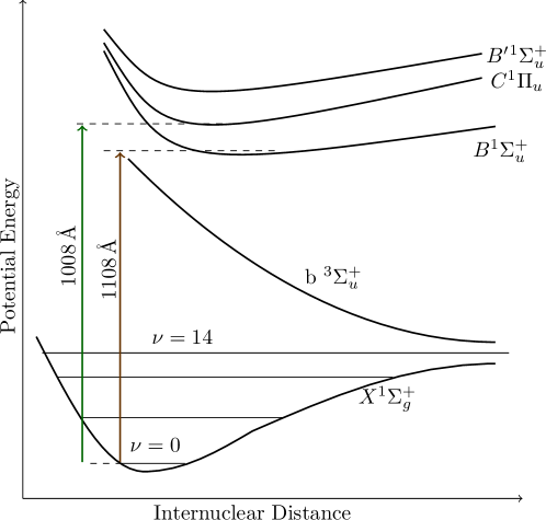
Figure 2: Schematic Born-Oppenheimer diagram for a hydrogen molecule (not to scale). The potential energy and the internuclear distance are given in arbitrary units. The ground state has 14 vibrational states which characterize the motion of the nuclei, while the excited $B{}^{1}\Sigma_{u}^{+}$ and $C{}^{1}\Pi_{u}$, and $B^{\prime}{}^{1}\Sigma_{u}^{+}$ states also harbor a number of vibrational sublevels.

5.2 Molecular Spectrum

A short description of the molecular spectrum of the $H_{2}$ molecule is in order. Binding into $\Sigma$ states starts from two hydrogen atoms in the ground state with orbital angular momenta $L_{1,2}=0$ and electronic spin angular momenta $S_{1,2}=1/2$. As a result, the projection of the total angular momentum onto the molecular axis is $\Lambda=L_{1}+L_{2}=0$, and the total spin quantum number is $S=0,1$. The first two excited states of $\Sigma$ symmetry, above the molecular ground state $X^{1}\Sigma_{g}^{+}$, are $B{}^{1}\Sigma_{u}^{+}$ and $B^{\prime}{}^{1}\Sigma_{u}^{+}$. The spin-triplet $b{}^{3}\Sigma_{u}^{+}$ state is not bonding. Even if the $b{}^{3}\Sigma_{u}^{+}$ state were bonding, we could ignore it because singlet to triplet transitions are forbidden by non-relativistic dipole selection rules [38]. Electronic dipole transitions from the excited $B{}^{1}\Sigma_{u}^{+}$ and $C{}^{1}\Pi_{u}$ states of H₂ molecule (see Fig. 2) to the ground state $X^{1}\Sigma_{g}^{+}$ were first observed by Lyman and Werner, and are therefore called the Lyman and Werner bands [39, 40, 41, 42].

The transition from the ground state $X{}^{1}\Sigma_{g}^{+}$ to the $B{}^{1}\Sigma_{u}^{+}$ state occurs at 1108Å  $\simeq$ 11.18991 eV, while the $X{}^{1}\Sigma_{g}^{+}$–$C{}^{1}\Pi_{u}^{+}$ transition occurs at 1008Å = 12.30002 eV (see Ref. [43]). These figures exclude possible vibrational and rotational excitations. The $1S$–$4P_{1/2}$ transition of atomic hydrogen occurs at 12.74851 eV, while the $1S$–$4P_{3/2}$ transition energy is 12.74852 eV (see Ref. [31]). Note that the $1S$–$4P_{1/2}$ and $1S$–$4P_{3/2}$ transition energies differ only by the fine-structure (which, in this case, enters at the seventh decimal). Indeed, the fine-structure splitting is an effect of relative order $\alpha^{2}$ (see Ref. [25]). The difference of the atomic $1S$–$4P_{1/2}$ transition energy to the $X$–$B$ and $X$–$C$ transitions is at least 0.4485 eV, provided no vibrational excitation occurs. For comparison, the transition energies for the $2S$–$4P_{1/2}$ and $3S$–$4P_{1/2}$ transitions [31] of atomic hydrogen are, respectively, 2.5497 eV and 0.6610 eV.

These considerations exclude vibrational and rotational excitations. In general, the ro-vibrational energy of a molecule is given as

$$E(\nu,J) = \left(\nu+\frac{1}{2}\right)\omega_{e}-\left(\nu+\frac{1}{2}\right)^{2}x_{e}\omega_{e}$$ (6ghyajbabcbebmcxcydedgdhdidjdkdldmdndodz)

$$+B_{\nu}J(J+1)-D_{J}J^{2}(J+1)^{2}\,,$$

where $\nu$ is the vibrational, and $J$ is the rotational quantum number. Here, $x_{e}\omega_{e}$ is the first-order anharmonic correction to the harmonic oscillator approximation to molecular vibration. The constant $B_{\nu}$,

$$B_{\nu}=B_{e}-\alpha_{e}\left(\nu+\frac{1}{2}\right)\,,$$ (6ghyajbabcbebmcxcydedgdhdidjdkdldmdndoea)

is the rotational constant for a given vibrational state. Here, $B_{e}$ is the rotational constant in the equilibrium position, and $\alpha_{e}$ is the first-order anharmonicity correction to the rotational constant. Finally, $D_{J}$ in Eq. (6ghyajbabcbebmcxcydedgdhdidjdkdldmdndodz) is the centrifugal distortion constant, several orders of magnitude smaller than $B_{\nu}$. To a first approximation, we can assume that the molecular vibration is of harmonic oscillator type, and centrifugal distortions of the rotational levels is negligible. More explicitly,

$$E(\nu,J)\simeq\left(\nu+\frac{1}{2}\right)\omega_{e}+B_{\nu}\,J(J+1)\,.$$ (6ghyajbabcbebmcxcydedgdhdidjdkdldmdndoeb)

Allowed ro-vibrational transitions have $\Delta J=0,\pm 1,\pm 2$. The $\Delta J=0$ transitions ($\Delta\nu\neq 0$) is the Raman $Q$-branch, while the R-branch and P-branches correspond to the $\Delta J=+1$ and $\Delta J=-1$ transitions, and are relevant for pure rotational spectroscopy. For diatomic molecules, in Raman transitions, the selection rules imply that the allowed transitions have $\Delta J=+2$ and $\Delta J=-2$ (Stokes and anti-Stokes lines, so-called S and O branches). Transitions with $|\Delta J|>2$ are forbidden by selection rules [38]. Here, we are neither concerned with pure rotational spectroscopy, nor with Raman spectroscopy, but with the inclusion of the ro-vibrational transitions into the sum-over-states representation of the $C_{6}$ coefficient according to Eq. (6ghyajbabcbebmcxcydedgdhdidjdkdldmdndodx). In order to discern the allowed rotational transitions from the $X$ to the $B$ and $C$ states, one needs to observe that the $X$ state is gerade, while $B$ and $C$ are ungerade. For the molecular ground state, it is well known that, if the proton spins in H₂ are antiparallel (total proton spin zero), then the spin wave function is antisymmetric under particle (proton) interchange, so that the orbital proton wave function must be symmetric under particle (proton) interchange, resulting in even values for $J$ (para-hydrogen). By contrast, if the proton spins in H₂ are parallel (total proton spin one), then the spin wave function is symmetric under particle (proton) interchange, and the orbital proton wave function must be anti-symmetric under particle (proton) interchange, resulting in odd values for $J$ (ortho-hydrogen). This holds because the ground-state two-electron wave function is gerade, while the required proton wave function symmetry is reversed for the $B$ and $C$ states, which are ungerade (see Ref. [44]). One can understand the symmetries most easily if one considers the molecular wave function in the Born–Oppenheimer approximation [42].

We have thus shown that the virtual transitions entering the expression (6ghyajbabcbebmcxcydedgdhdidjdkdldmdndodx) have $\Delta J=\pm 1$ if the transition involves gerade and ungerade states of the hydrogen molecule. Let us try to analyze the frequency shift in a virtual transitions of H₂, due to the addition of a rotational quantum. We anticipate that, because of the small magnitude of the effect, it is sufficient to study the frequency shift within a given manifold of rotational states, specific to either the initial or the final state of the virtual transition. The energy differences for $J\to J+1$ transitions, within a given vibrational band, read as

$$\Delta E(\nu,J)=E(\nu,J+1)-E(\nu,J)\simeq 2B_{\nu}\,(J+1)\,.$$ (6ghyajbabcbebmcxcydedgdhdidjdkdldmdndoec)

The difference between rotational lines in a vibrational band is thus $\Delta E(\nu,J+1)-\Delta E(\nu,J)=2B_{\nu}$, which means the ro-vibrational transition energies increase equally by an amount of $2B_{\nu}$ in both $\Delta J=\pm 1$. For the $X{}^{1}\Sigma_{g}^{+}$ state, the rotational $B_{e}$ and $\alpha_{e}$ constants are $B_{e}=60.853\,\mathrm{cm}^{-1}$ and $\alpha_{e}=3.062\,\mathrm{cm}^{-1}$, respectively (see Ref. [42]). Thus, the $B_{\nu}$ coefficient of the $X{}^{1}\Sigma_{g}^{+}$ state for the vibrational ground state is $7.355\times 10^{-3}\,\mathrm{eV}$.

5.3 Possible Enhancement of the van der Waals Coefficient

We have already stressed that the difference of the atomic $1S$–$4P$ transition to the $X$–$B$ and $X$–$C$ transitions of H₂ is at least 0.4485 eV, thus setting a lower limit for the magnitude of the propagator denominator given in Eq. (6ghyajbabcbebmcxcydedgdhdidjdkdldmdndody). Two effects could lead to an enhancement of $C_{6}$. (i) One might assume that the ground-state hydrogen molecule enters the collision with atomic hydrogen, in a thermally excited rotational state, thus modifying the transition frequencies to virtual excited states of the molecule, and (ii) potential virtual transitions from the $X$ ground state of H₂ to rotational sidebands of the vibrational levels $\nu=11$ of the $B$, and $\nu=2$ of the $C$, state, could potentially enhance $C_{6}$.

Let us try to address point (i). At a temperature of $T=5.8\,{\rm K}$, which is relevant for the experiment [13] the thermal excitation energy is $k_{B}T=4.998\times 10^{-4}\,\mathrm{eV}$. (In general, high-precision atomic-beam experiments profit enormously from cryogenic beams.) Equating the thermal excitation energy with the rotational energy, one can obtain an estimate for the typical rotational $J$ value due to thermal excitation, assuming a Boltzmann distribution,

$$J\,(J+1)-\frac{4.998\times 10^{-4}\mathrm{eV}}{7.355\times 10^{-3}\,\mathrm{eV}}=0\Rightarrow J=0.06\,.$$ (6ghyajbabcbebmcxcydedgdhdidjdkdldmdndoed)

This implies that the thermal energy is insufficient to excite rotational levels, leaving the molecular ground state $X{}^{1}\Sigma_{g}^{+}$ of the system in the rotational ground state of the $\nu=0$ vibrational band. Thus, we can safely assume that all collisions involving H₂ molecules start from the rotational ground state, i.e., from a para-hydrogen state (after thermalization).

Having excluded thermal excitation of the ground state as a further source of a quasi-degeneracy of transitions in our system, we must now exclude point (ii), namely, the possibility of virtual transitions, from the rotational ground state of the hydrogen molecule, to higher vibrational and rotational sublevels of the $B$ and $C$ states, which could otherwise drastically reduce the energy difference with respect to the hydrogen $1S$–$4P$ transition, and decrease the magnitude of the quantity $E_{nm}^{(A)}+E_{n^{\prime}m^{\prime}}^{(B)}$ in Eq. (6ghyajbabcbebmcxcydedgdhdidjdkdldmdndody). We recall that the energy difference between the atomic $1S$–$4P$ transition and the $X$–$B$ molecular transition is 1.5589 eV. The $\nu=11$ vibrational sublevel of the $B{}^{1}\Sigma_{u}^{+}$ state of molecular hydrogen has an energy of 102856.97 cm${}^{-1}\simeq$ 12.7526 eV (see Table I of Ref. [45]), which is closest to the $1S$–$4P$ transition of 12.7485 eV, among all vibrational levels but higher in energy than the atomic hydrogen line, so that the degeneracy cannot be reduced by adding rotational quanta. For the $B$ transition, in order to address the possibility of rotationally induced quasi-degeneracy, one should also note the $\nu=10$ vibrational sublevel of the $B{}^{1}\Sigma_{u}^{+}$ state of molecular hydrogen has an energy of 101864.90 cm${}^{-1}\simeq$ 12.6296 eV (see Table I of Ref. [45]). On the other hand, we recall once more that the energy difference between the atomic $1S$–$4P$ transition and $X$–$C$ transition in molecular hydrogen is 0.4485 eV. The $\nu=2$ vibrational sublevel of the $C{}^{1}\Pi_{u}$ state of molecular hydrogen has an energy of 103628.662 cm${}^{-1}\simeq$ 12.84830 eV (see Table 5 of Ref. [46]), which is very close to the $1S$–$4P$ transition of 12.7485 eV and energetically closest among the different vibrational levels. As an inspection shows, it is also higher in energy than the atomic hydrogen line, so that the degeneracy cannot be reduced by adding rotational quanta. For the $X$–$C$ transition, in order to address the possibility of rotationally induced quasi-degeneracy, one should also note the $\nu=1$ vibrational sublevel of the $C{}^{1}\Pi_{u}$ state of molecular hydrogen has an energy of 101457.569 cm${}^{-1}\simeq$ 12.5791 eV (see Table 5 of Ref. [46]).

One can argue as follows. The rotational energy roughly follows $J(J+1)\approx J^{2}$, for large $J$ [see Eq. (6ghyajbabcbebmcxcydedgdhdidjdkdldmdndoeb)]. For the $X$–$B$ transition, to achieve quasi-degeneracy of about $1.189\times 10^{-1}\,\mathrm{eV}$ with $B_{\nu}\sim 9.395\times 10^{-4}\,\mathrm{eV}$, we need $J^{2}\sim 127\Rightarrow J\sim 11$. Likewise, for the $X$–$C$ transition, in order to achieve quasi-degeneracy by adding rotational excitation energy of the excited H₂ state of about $1.694\times 10^{-1}\,\mathrm{eV}$ with $B_{\nu}\sim 3.579\times 10^{-3}\,\mathrm{eV}$, we need $J^{2}\sim 47\Rightarrow J\sim 7$. By symmetry considerations, one can show that relevant rotational transitions in our system need to satisfy $\Delta J=\pm 1$. Transitions with $\Delta J=+1$ bring the $X$–$B$ and the $X$–$C$ transitions closer to the $1S$–$4P_{1/2}$ atomic transition only by 0.1% and 1.5% respectively. With a forbidden transition featuring $\Delta J=+2$, one can bring the $X$–$B$ and the $X$–$C$ transitions closer to the $1S$–$4P$ atomic transition only by the insignificant amounts of 0.3% and 4.5%, respectively. Effects due to higher multipoles, which could potentially lead to “even more forbidden” transitions, are typically suppressed by powers of $\alpha$ [47, 48], with one power of $\alpha$ for each higher angular momentum involved. For the very high required $\Delta J$ values, the contribution from the transitions which involve the “highly forbidden $\Delta J$” is thus numerically suppressed and can safely be neglected.

5.4 Estimate of the van der Waals Coefficient

The remaining task is to find the oscillator strength of excitation from the ground $X{}^{1}\Sigma_{g}^{+}$ molecular state to the $\nu=11$ vibrational side band of the excited $B{}^{1}\Sigma_{u}^{+}$ molecular state, and the same for the relevant $X$–$C$ transition. The oscillator strength for the $\nu=11$ vibrational band of the Lyman band is given in Ref. [49, 50] and reads and $f=1.74\times 10^{-2}\,{\rm a.u.}$, while the oscillator strength for $\nu=2$ vibrational band of the Werner band is $f^{\prime}=6.95\times 10^{-2}\,{\rm a.u.}$ (see Refs. [49, 50]). For comparison, slightly discrepant oscillator strengths are given in Refs. [51] and [52], for the $\nu=2$ vibrational band of $C$, namely, $f^{\prime}=5.55\times 10^{-2}$ and $f^{\prime}=6.42\times 10^{-2}$, respectively. We here use the oscillator strength reported in Ref. [49] in our estimate. The oscillator strength for the $4P$–$1S$ atomic hydrogen transition is $-9.66\times 10^{-3}$ [see Eq. (6ghyajbabcbebmcxcydedgdhdidjdkdldmdndodv)]. Consequently, the contribution of the virtual vibrational sublevels of the $B$ and $C$ states of H₂, which are closest-in-energy to the $1S$-$4P$ transition in H, are given as

$$C_{6}(X;B)\approx\frac{3}{2}\;\frac{(-9.66\times 10^{-3})\times 1.74\times 10^{-2}}{(-0.4685)\times 0.4686\times 1.499\times 10^{-4}}=7.661\;\mathrm{a.u.}\,,$$ (6ghyajbabcbebmcxcydedgdhdidjdkdldmdndoee)

$$C_{6}(X;C)\approx\frac{3}{2}\;\frac{(-9.66\times 10^{-3})\times 6.95\times 10^{-2}}{(-0.4685)\times 0.4722\times 3.667\times 10^{-3}}=1.241\;\mathrm{a.u.}\,.$$ (6ghyajbabcbebmcxcydedgdhdidjdkdldmdndoef)

The sum is $C_{6}(X;B)+C_{6}(X;C)$ is $\sim 8.901$ in atomic units. The energies in the denominator of Eqs. (6ghyajbabcbebmcxcydedgdhdidjdkdldmdndoee) and (6ghyajbabcbebmcxcydedgdhdidjdkdldmdndoef) are expressed in terms of the atomic unit of energy, namely, the Hartree energy $E_{h}=27.2114\,{\rm eV}$, using the unit conversion of $1\,{\rm eV}=0.0367493E_{h}$. As a last step, one needs to consider $X$–$B^{\prime}$ transitions. Neglecting rotational quanta, the $X$–$B^{\prime}$ transition is at 110529.47 cm${}^{-1}\simeq 13.704$ eV (see Table 5 of [53]), while the $X$–$D$ transition is at 1129335.29 cm${}^{-1}\simeq 14.002$ eV (see Table 7 of [53]). These transition energies exceed the ionization threshold of atomic hydrogen. Considering the $X$–$B^{\prime}$ and $X$–$D$ transitions in the H₂ molecule and the $4P$–$1S$ transition in atomic hydrogen, the propagator denominator (6ghyajbabcbebmcxcydedgdhdidjdkdldmdndody) becomes positive, and, in magnitude, greater than the $4P$ atomic hydrogen binding energy. Consequently, the contribution of the $B^{\prime}$ and the $D$ states to the van der Waals $C_{6}$ coefficient in the H($4P$)–H₂ interactions is opposite in sign to that of $B$ and $C$ molecular states; numerically, it is small in magnitude in comparison to $C_{6}(X;B)$ and $C_{6}(X;C)$. Because the involved virtual transition frequencies and oscillator strengths are independent of the hydrogen fine structure, to the order of the approximations made, the result is the same for both $4P_{1/2}$ and $4P_{3/2}$ reference states. We can thus safely neglect the possibility of a dramatic enhancement of the $C_{6}$ coefficient in collisions of hydrogen molecules with $4P$ hydrogen atoms. The total magnitude of the $C_{6}$ coefficient will be determined by non-quasi-degenerate states, i.e., by a sum over the entire bound and continuous spectrum of the hydrogen atoms and molecules, as given by the general formula (6ghyajbabcbebmcxcydedgdhdidjdkdldmdndodx). Based on typical calculations available for other atomic and molecular systems without quasi-degeneracies [37], we can thus conservatively estimate that

$$|C_{6}(4P\,{\rm H};X{}^{1}\Sigma^{+}_{g}\,{\rm H}_{2})|\leq 20\,{\rm a.u.}\,.$$ (6ghyajbabcbebmcxcydedgdhdidjdkdldmdndoeg)

Let us now turn to the H–H₂ interaction for the planned $1S$–$6P$ experiment [54]. The $6P$–$1S$ transition energy of about $13.22068\,$eV [31] is comparable to the $X$–$B(\nu=15)$ transition energy of 106534.3  cm${}^{-1}\simeq 13.2085\,$eV [55] and the $X$–$C(\nu=4)$ transition energy of 107580.936 cm${}^{-1}\simeq 13.3383\,$eV (see Ref. [46]). The binding energy of the $6P$-level of atomic hydrogen is less than that of the $4P$-level. We notice that the $X$–$B(\nu=15)$ transition energy is below the atomic $6P$–$1S$ transition energy (in absolute magnitude), while the magnitude of the $X$–$C(\nu=4)$ transition energy exceeds that of the atomic $6P$–$1S$ energy difference. For the same reasons as given above for $4P$ interactions, the $B^{\prime}{}^{1}\Sigma_{u}^{+}$ and $D{}^{1}\Pi_{u}$ molecular levels lead to negligible contributions to the $C_{6}$ coefficient for H($6P$)–H₂ interactions. The oscillator strength of the $\nu=15$ vibrational level of the molecular $B$ state and the $\nu=4$ vibrational level of the molecular $C$ state are, respectively, $7.94\times 10^{-3}$ and $3.87\times 10^{-2}$ in atomic units [49]. The oscillator strength for the $6P_{j}$–$1S$ transition, where $j$ takes either $1/2$ or $3/2$, is $-2.60\times 10^{-3}$. As a result, the $C_{6}$ coefficient of the H($6P$)–H₂ interactions reads $C_{6}=2\times(-0.293+0.147)\,{\rm a.u.}=-0.292\,{\rm a.u.}$. Just as for $4P$ hydrogen, the total magnitude of the $C_{6}$ coefficient will be determined by non-quasi-degenerate states. molecules, as given by the general formula (6ghyajbabcbebmcxcydedgdhdidjdkdldmdndodx). Based on typical calculations available for other atomic and molecular systems without quasi-degeneracies [37], we can thus conservatively estimate that

$$|C_{6}(6P\,{\rm H};X{}^{1}\Sigma^{+}_{g}\,{\rm H}_{2})|\leq 20\,{\rm a.u.}\,.$$ (6ghyajbabcbebmcxcydedgdhdidjdkdldmdndoeh)

Both estimates (6ghyajbabcbebmcxcydedgdhdidjdkdldmdndoeg) and (6ghyajbabcbebmcxcydedgdhdidjdkdldmdndoeh) are smaller than the $C_{6}$ coefficients obtained for atom-atom collisions, discussed in Secs. 3 and 4.

6 Conclusions

We have studied the van der Waals interaction of excited $4P$ hydrogen atoms with ground-state $1S$ and metastable $2S$ atoms, and with hydrogen molecules. In order to obtain reliable estimates of the van der Waals interaction coefficients, one needs to expand the states in a hyperfine-resolved basis, and consider all off-diagonal matrix elements of the van der Waals interaction Hamiltonian, as outlined in Secs. 2.1 and 2.2. The explicit construction of the hyperfine-resolved states is discussed in Sec. 2.3, and the use of the Wigner–Eckhart theorem for the calculation of the matrix elements of the van der Waals interaction is described in Sec. 2.4.

For the $4P$–$1S$ system, one needs to include both the $4P_{1/2}$ as well as the $4P_{3/2}$ states in the quasi-degenerate basis, because the $4P$ fine-structure frequency is commensurate with the $1S$ hyperfine transition splitting (see Sec. 3.1). The matrix elements of the total Hamiltonian involve the so-called hyperfine–fine–structure mixing term (see Sec. 3.2), which couples the $4P_{1/2}(F=1)$ to the $4P_{3/2}(F=1)$ levels [see Eq. (6ghyajav)].

The explicit matrices of the total Hamiltonian (5) in the manifolds with ${\mathfrak{F}}_{z}=3,2,1$ are described in Secs. 3.3—3.5. Final results are also indicated for the (otherwise excessively complex) manifold with ${\mathfrak{F}}_{z}=0$. Due to mixing terms of first order in the van der Waals interaction between degenerate states in the two-atom system, the leading term in the van der Waals energy, upon rediagonalization of the Hamiltonian matrix, is of order $1/R^{3}$ for the $4P$–$1S$ interaction, but it averages out to zero over the magnetic projections. The phenomenologically important second-order shifts of the energy levels are given in Sec. 3.6, with various averaging procedures illustrating the dependence of the shifts on the quantum numbers, and the dependence of the repulsive or attractive character of the interaction on the hyperfine-resolved levels.

The same procedure is applied to the $4P$–$2S$ interaction in Sec. 4, with the additional complication that virtual quasi-degenerate $(4S;2P_{1/2})$ also need to be included in the basis. The treatment of the $4P$–$1S$ and $4P$–$2S$ long-range interactions reveals the presence of numerically large coefficients multiplying the $1/\rho^{6}$ interaction terms, due to the presence of quasi-degenerate levels. The interaction remains nonretarded over all phenomenologically relevant distance scales.

For atom-molecule collisions, the analysis has been carried out in Sec. 5. After some general considerations which illustrate the complications that can arise for excited states (see Sec. 5.1), we briefly discuss the molecular spectrum (Sec. 5.2), before discussing possible enhancement mechanisms for the van der Waals coefficient, which can be of thermal and other origin (see Sec. 5.3). A numerical estimate of the coefficient is performed in Sec. 5.4, with the result that the drastic enhancement that we see in atom-atom collisions, is in fact absent for atom-molecular interactions. This observation is of high relevance to the analysis of experiments.

References

- [1] M. I. Chibisov, Dispersion Interaction of Neutral Atoms, Opt. Spectrosc. 32, 1–3 (1972).
- [2] W. J. Deal and R. H. Young, Long–Range Dispersion Interactions Involving Excited Atoms; the H(1s)—H(2s) Interaction, Int. J. Quantum Chem. 7, 877–892 (1973).
- [3] C. M. Adhikari, V. Debierre, A. Matveev, N. Kolachevsky, and U. D. Jentschura, Long-range interactions of hydrogen atoms in excited states. I. – interactions and Dirac– perturbations, Phys. Rev. A 95, 022703 (2017).
- [4] U. D. Jentschura, V. Debierre, C. M. Adhikari, A. Matveev, and N. Kolachevsky, Long-range interactions of excited hydrogen atoms. II. Hyperfine-resolved – system, Phys. Rev. A 95, 022704 (2017).
- [5] E. A. Power and T. Thirunamachandran, Dispersion forces between molecules with one or both molecules excited, Phys. Rev. A 51, 3660–3666 (1995).
- [6] H. Safari, S. Y. Buhmann, D.-G. Welsch, and H. T. Dung, Body-assisted van der Waals interaction between two atoms, Phys. Rev. A 74, 042101 (2006).
- [7] H. Safari and M. R. Karimpour, Body-Assisted van der Waals Interaction between Excited Atoms, Phys. Rev. Lett. 114, 013201 (2015).
- [8] P. R. Berman, Interaction energy of nonidentical atoms, Phys. Rev. A 91, 042127 (2015).
- [9] P. W. Milonni and S. M. H. Rafsanjani, Distance dependence of two-atom dipole interactions with one atom in an excited state, Phys. Rev. A 92, 062711 (2015).
- [10] M. Donaire, R. Guérout, and A. Lambrecht, Quasiresonant van der Waals Interaction between Nonidentical Atoms, Phys. Rev. Lett. 115, 033201 (2015).
- [11] M. Donaire, Two-atom interaction energies with one atom in an excited state: van der Waals potentials versus level shifts, Phys. Rev. A 93, 052706 (2016).
- [12] U. D. Jentschura, C. M. Adhikari, and V. Debierre, Virtual Resonant Emission and Long–Range Tails in van der Waals Interactions of Excited States: QED Treatment and Applications, Phys. Rev. Lett. 118, 123001 (2017).
- [13] A. Beyer, L. Maisenbacher, A. Matveev, R. Pohl, K. Khabarova, A. Grinin, T. Lamour, D. C. Yosta, T. W. Hänsch, N. Kolachevsky, and T. Udem, The Rydberg constant and proton size from atomic hydrogen, Science 358, 79–85 (2017).
- [14] S. Wolfram, The Mathematica Book, 4 ed. (Cambridge University Press, Cambridge, UK, 1999).
- [15] S. Jonsell, A. Saenz, P. Froelich, R. C. Forrey, R. Côté, and A. Dalgarno, Long-range interactions between two 2s excited hydrogen atoms, Phys. Rev. A 65, 042501 (2002).
- [16] A. Matveev, N. Kolachevsky, C. M. Adhikari, and U. D. Jentschura, Pressure Shifts in High–Precision Hydrogen Spectroscopy. II. Impact Approximation and Monte–Carlo Simulations, submitted (2018).
- [17] R. Pohl, private communication (2017).
- [18] T. Udem, private communication (2017).
- [19] U. D. Jentschura and C. M. Adhikari, Long–Range Interactions for Hydrogen: – and – Systems, Atoms 5, 48 (2017).
- [20] D. J. Berkeland, E. A. Hinds, and M. G. Boshier, Precise Optical Measurement of Lamb Shifts in Atomic Hydrogen, Phys. Rev. Lett. 75, 2470–2473 (1995).
- [21] P. J. Mohr, D. B. Newell, and B. N. Taylor, CODATA Recommended Values of the Fundamental Physical Constants: 2014, Rev. Mod. Phys. 88, 035009 (2016).
- [22] C. M. Adhikari, V. Debierre, and U. D. Jentschura, Adjacency graphs and long-range interactions of atoms in quasi-degenerate states: applied graph theory, Appl. Phys. B 123, 1 (2017).
- [23] A. Salam, Non-Relativistic QED Theory of the van der Waals Dispersion Interaction (Springer, Cham, Switzerland, 2016).
- [24] C. M. Adhikari, Ph.D. thesis, Missouri University of Science and Technology, Rolla, MO, 2017 (unpublished).
- [25] C. Itzykson and J. B. Zuber, Quantum Field Theory (McGraw-Hill, New York, 1980).
- [26] A. R. Edmonds, Angular Momentum in Quantum Mechanics (Princeton University Press, Princeton, New Jersey, 1957).
- [27] D. M. Brinks and G. R. Satchler, Angular Momentum (Oxford University Press, Oxford, 1994).
- [28] L. D. Landau and E. M. Lifshitz, Quantum Mechanics, Volume 3 of the Course on Theoretical Physics (Pergamon Press, Oxford, UK, 1958).
- [29] H. A. Bethe and E. E. Salpeter, Quantum Mechanics of One- and Two-Electron Atoms (Springer, Berlin, 1957).
- [30] M. Horbatsch and E. A. Hessels, Tabulation of the bound-state energies of atomic hydrogen, Phys. Rev. A 93, 022513 (2016).
- [31] For an interactive database of hydrogen and deuterium transition frequencies, see the URL http://physics.nist.gov/hdel.
- [32] N. Kolachevsky, A. Matveev, J. Alnis, C. G. Parthey, S. G. Karshenboim, and T. W. Hänsch, Measurement of the Hyperfine Interval in Atomic Hydrogen, Phys. Rev. Lett. 102, 213002 (2009).
- [33] S. R. Lundeen and F. M. Pipkin, Measurement of the Lamb Shift in Hydrogen, , Phys. Rev. Lett. 46, 232–235 (1981).
- [34] K. Pachucki, Theory of the Lamb shift in muonic hydrogen, Phys. Rev. A 53, 2092–2100 (1996).
- [35] A. R. Edmonds, Angular Momentum in Quantum Mechanics (Princeton University Press, Princeton, New Jersey, 1974).
- [36] W. L. Wiese and J. R. Fuhr, Accurate Atomic Transition Probabilities for Hydrogen, Helium, and Lithium, J. Phys. Chem. Ref. Data 38, 565–720 (2009).
- [37] A. Dalgarno, I. H. Morrison, and R. M. Pengelly, Long-Range Interactions Between Atoms and Molecules, Int. J. Quantum Chem. 1, 161–167 (1967).
- [38] G. Herzberg, Spectra of diatomic molecules (Van Nostrand Reinhold, Princeton, MA, 1959).
- [39] T. Lyman, The Spectrum of Hydrogen in the Region of Extremely Short Wave–Length, Astrophys. J. 23, 181–210 (1906).
- [40] S. Werner, Hydrogen Bands in the Ultra–Violet Lyman Region, Proc. Roy. Soc. London, Ser. A 113, 107–117 (1926).
- [41] G. Herzberg and L. L. Howe, The Lyman bands of molecular hydrogen, Can. J. Phys. 37, 636–659 (1959).
- [42] W. Heitler, Quantum Theory of Radiation (Oxford University Press, New York, 1950).
- [43] G. B. Field, W. B. Somerville, and K. Dressler, Hydrogen Molecules in Astronomy, Ann. Rev. Astron. Astrophysics 4, 207 (1966).
- [44] M. J. S. Dewar and J. Kelemen, LCAO MO Theory Illustrated by Its Application to H2, J. Chem. Edu. 48, 494–501 (1971).
- [45] A. F. Starace, Comment on “Length and Velocity Formulas in Approximate Oscillator–Strength Calculations”, Phys. Rev. A 8, 1141–1142 (1973).
- [46] J. Philip, J. P. Sprengers, T. Pielage, C. A. de Lange, W. Ubachs, and E. Reinhold, Highly accurate transition frequencies in the H 2 Lyman and Werner absorption bands, Can. J. Chem. 82, 713–722 (2004).
- [47] Z. C. Yan, J. F. Babb, A. Dalgarno, and G. W. F. Drake, Variational calculations of dispersion coefficients for interactions among H, He, and Li atoms, Phys. Rev. A 54, 2824–2833 (1996).
- [48] G. Łach, M. DeKieviet, and U. D. Jentschura, Multipole Effects in Atom–Surface Interactions: A Theoretical Study with an Application to He–-quartz, Phys. Rev. A 81, 052507 (2010).
- [49] W. F. Chan, G. Cooper, and C. E. Brion, Absolute optical oscillator strengths (11-20 eV) and transition moments for the photoabsorption of molecular hydrogen in the Lyman and Werner bands, Chem. Phys. 168, 375–388 (1992).
- [50] A. C. Allison and A. Dalgarno, Band oscillator strengths and transition probabilities for the Lyman and Werner systems of H2, HD, and D2, At. Data Nucl. Data Tables 1, 289–304 (1969).
- [51] J. Geiger and H. Schmoranzer, Electronic and vibrational transition probabilities of isotopic hydrogen molecules H2, HD, and D2 based on electron energy loss spectra, J. Mol. Spect. 32, 39–53 (1969).
- [52] W. Fabian and B. R. Lewis, Experimentally determined oscillator strengths for molecular hydrogen-I. The Lyman and Werner bands above 900Å, J. Quant. Spectry. Rad. Transfer 14, 523–535 (1974).
- [53] H. Abgrall, E. Roueff, F. Launay, and J.-Y. Roncin, The and band systems of molecular hydrogen, Can. J. Phys. 72, 856–865 (1994).
- [54] T. Udem and T. W. Hänsch, private communication (2017).
- [55] W. C. Stwalley, Potential energy curve of the state of H, J. Chem. Phys. 58, 536–540 (1973).