Superfluids, Fluctuations and Disorder

Abstract

We present a field-theory description of ultracold bosonic atoms in presence of a disordered external potential. By means of functional integration techniques, we aim to investigate and review the interplay between disordered energy landscapes and fluctuations, both thermal and quantum ones. Within the broken-symmetry phase, up to the Gaussian level of approximation, the disorder contribution crucially modifies both the condensate depletion and the superfluid response. Remarkably, it is found that the ordered (i.e. superfluid) phase can be destroyed also in regimes where the random external potential is suitable for a perturbative analysis. We analyze the simplest case of quenched disorder and then we move to present the implementation of the replica trick for ultracold bosonic systems. In both cases, we discuss strengths and limitations of the reviewed approach, paying specific attention to possible extensions and the most recent experimental outputs.

I Introduction

Ultracold atomic gases have been the cornerstone of atomic physics since 1995 cornell-1995 ; ketterle-1995 , when Bose-Einstein condensation was experimentally achieved for the first time. This groundbreaking result was the starting point of an ongoing and intense research effort to improve atoms trapping and cooling procedures pethick-book . Nowadays, modern laboratories have reached an exquisite control on the relevant physical parameters for atomic gases, such as the number density or the strength and range of atom-atom interaction. At the same time, it is also possible to tune the coupling with the external environement, enabling the observation of quantum dynamics without spurious smearing effects langen-2015 .

It is then natural to think of ultracold atomic gases as an extremely effective platform to probe quantum theories up to the macroscopic scale. One of the most striking example is given by the Bose-Hubbard model and its superfluid-insulator transition originally predicted in fisher-1989 . This quantum phase transition was first observed in 2002 by loading a repulsive condensate in an optical lattice confining potential greiner-2002 . Similar achievements have been reached for low-dimensional quantum gases and their remarkable phenomenology giamarchi-book ; dalibard-review-2d . Among a wide and interesting literature, it is worth mentioning the first direct observation of the Tonks-Girardeau regime in an optical lattice filled with alkali atoms paredes-2004 ; kinoshita-2004 or the vortex proliferation associated to the Berezinskii-Kosterlitz-Thouless physics in two-dimensional setups hadzibabic-2006 ; cornell-2007 . More recently, a growing interest has aroused on cold atoms as a promising quantum simulation platform. Together with the refined experimental expertise, it has been shown that, within peculiar setups, the superfluid dynamics of atoms obeys to equations which can be mapped to other ones appearing in high-energy physics or cosmology. For instance, Rabi-coupled bosonic mixtures seem to be a burgeoning candidate to explore inflationary dynamics and space-time expansion in table top experiments marquardt-2015 ; brandt-2017 ; braden-2018 . Other proposals involve cold-atoms analog of quantum gravity liberati-2006 or the implementation of system mimicking QCD features sademelo-2018 .

Restraining ourselves to the condensed matter domain, ultracold atoms offer the interesting possibility to investigate the intriguing issue of quantum transport in a disordered environment kamenev-review . Indeed, from the dawn of solid state theory it was clear that a well-founded investigation has to consider the multifaceted role played by microscopic impurities and disordered external potential. For instance, common incandescent lamp would not exist without a certain degree of impurity scattering. At the same time, it is reasonable to expect a smearing of experimental data due to randomly wrinkled substrate or the destruction of supertransport properties. Examples of this parasitic role can be traced back to dirty superconductors or ⁴He diffusion in porous medium ma-1985 ; ma-1986 . The complexity of this problem lies in the interplay between superfluidity (i.e. the occuring of some kind of ordered phase) and the localization phenomenon first theorized by Anderson in anderson-1959 .

Given the broad interest and the cross-disciplinary relevance of this problem, it is reasonable to turn towards cold atoms, since they offer reliable experimental protocols to engineer disordered external potential and control the corresponding relevant parameters. The dirty bosons problem then gathers all the investigations addressing the properties of ultracold bosons subject to an external random potential. The interplay between superfluidity and localization may lead to the observation of a new phase, the so-called Bose glass fisher-1989 . Similarly to the Bose-Hubbard model in absence of disorder, optical lattices have been proved again to be a reliable setup to explore these exotic features damski-2003 . While interfering counterpropagating beams create the first regular pattern, randomness is added by superimposing a second optical lattice, providing a viable strategy to control the degree of disorder schulte-2005 ; billy-2008 ; roati-2008 . An alternative is given by the speckle optical potential, generated by the interference of waves with different phases and amplitudes but with the same frequency dainty-1980 ; goodman-book . The resulting wave varies randomly in space and can be used to study the transport properties of ultracold atoms in presence of static external disorder lye-2005 ; clement-2005 ; ghabour-2014 .

In order to tackle down the crucial aspects of the dirty bosons problem, the relevant theoretical tools can be divided in two different subsets. At first, one can adopt the point of view of Bogoliubov theory, treating disorder in a perturbative way, similarly to quantum and thermal fluctuations in the pure system stoof-book ; salasnich-2016 . Since the first seminal work on this topic huang-1992 ; giorgini-1994 ; tauber-1997 , this approach has led us to a better understanding of the role played by disorder, no matter how small, in condensed bosonic systems. The additional depletion to condensate and superfluid was computed in huang-1992 , while in giorgini-1994 the authors investigated the modifications induced by a random external potential to the sound propagation. At the same time, critical properties are investigated by focusing, for instance, on the condensation temperature shift driven by the interplay of disorder and interaction lopatin-2002 ; falco-2007 .

A non-perturbative approach paves the way to the exploration of the superfluid-glass (quantum) transition in bosonic ensembles. Moving from the seminal renormalization-group analysis for one-dimensional systems giamarchi-1988 ; giamarchi-book , different strategies and methods have been used to understand the phase diagram of dirty bosons in three and lower dimensions, such as the random-phase approximation navez-2007 , stochastic field-theory techniques and the replica formalism yukalov-2007 ; falco-2009 ; khellil-2016 ; khellil-2016-2 .

The ambition of this review is obviously more limited, since it is not possible face in the main text all the topics we have mentioned during this introduction. Nevertheless, we aim to present, in a clear and pedagogical way, the crucial ingredients of a field-theory analysis of superfluid bosons. Throughtout the proceeding of the paper, we are going to adopt the functional integration framework, which is flexible enough to enable the implementation of different approximation schemes altland-book . Our discussion is organized in the following way: in Sec. II we specify how one can build up a quantum field theory for superfluid bosons subject to a random confinement. In particular, one needs to clarify the way in which disorder is introduced and characterized. In Sec. III we compute, up to the Gaussian level of approximation, the additional contribution to the condensate and the superfluid component due to the presence of a quenched disordered potential. Moving to Sec. IV, we present the core ideas at the foundation of the replica formalism, which allows to generalize our analysis to more complex disorder realization and does not rely, in principle, upon the assumption of a perturbatively small disorder. Within this scheme, we show how to compute the meaningful correlation functions and describe the superfluid response of the system in Sec. V. Further comments and future perspective are addressed in the Conclusions.

II Disorder in Field Theories

Let us begin by considering $N$ interacting bosonic particles of mass $m$ enclosed in a $L^{d}$ volume and subject to an external disordered potential $U_{\text{D}}(\mathbf{r})$. Thus, the Hamiltonian is simply given by

$$\hat{H}=\sum_{i=1}^{N}\bigg{[}-\frac{\hbar^{2}\nabla_{i}^{2}}{2m}+\hat{U}_{\text{D}}(\mathbf{r}_{i})\bigg{]}+\frac{1}{2}\sum_{i\neq j}\hat{V}\big{(}|\mathbf{r}_{i}-\mathbf{r}_{j}|\big{)}\;,$$ (1)

with $\hat{V}\big{(}|\mathbf{r}_{i}-\mathbf{r}_{j}|\big{)}$ the two-body central interaction potential. The thermodynamic description of the system can be derived from the partition function. Within the canonical ensemble, it is defined as

$$Z_{N}=\sum_{\{n\}}\exp\big{(}-\beta E_{n}\big{)}$$ (2)

where $\beta\equiv(k_{B}T)^{-1}$ and $\{n\}$ denoting the bosonic states (i.e. totally symmetric with respect to particle exchange) with eigenenergy $E_{n}$ of the operator $\hat{H}$ in Eq. (1). In order to adopt the functional integration formalism altland-book , Eq. (1) has to be expressed in second quantization. By adding $-\mu\hat{N}$, with $\mu$ the chemical potential and $\hat{N}$ the number operator, we can also move to the grand canonical ensemble. Here, a basis of coherent bosonic states can be chosen, leading to the imaginary-time representation of the (grand canonical) partition function

$$\mathscr{Z}=\int\mathscr{D}[\psi,\psi^{*}]\,e^{-S[\psi,\psi^{*}]/\hbar}\;.$$ (3)

In the equation above, the Bose statistics is encoded in the periodic boundary condition for the fields, namely $\psi(0)=\psi(\beta\hbar)$ and $\psi^{*}(0)=\psi^{*}(\beta\hbar)$. The Eucliden action appearing in Eq. (3) is given by

$$S[\psi,\psi^{*}] =\int_{0}^{\beta\hbar}d\tau\int d^{d}\mathbf{r}\;\bigg{\{}\psi^{*}(\mathbf{r},\tau)\bigg{[}\hbar\partial_{\tau}-\frac{\hbar^{2}\nabla^{2}}{2m}-\mu-U_{\text{D}}(\mathbf{r},\tau)\bigg{]}\psi(\mathbf{r},\tau)$$ (4)

$$\qquad\qquad\qquad\qquad\qquad+\frac{1}{2}\int d^{d}\mathbf{r}^{\prime}|\psi(\mathbf{r},\tau)|^{2}V(|\mathbf{r}-\mathbf{r}^{\prime}|)|\psi(\mathbf{r}^{\prime},\tau)|^{2}\bigg{\}}\;.$$

We have now to clarify what is meant by a (quantum) field theory for the disordered Bose gas. Also in the simplest case of non-interacting bosons, given a certain realization of the disordered confinement, an exact diagonalization of Eq. (1) does not appear as a feasible task.

A statistical approach is certainly more reasonable, since it allows, in principle, to characterize the system through a limited range of variables as, for instance, the strength of the impurity potential leading to the disorder, or the scale of space-time potential fluctuations. This obviously implies that it is possible to average (in a way to define) over different microscopic realization of the disorder potential.

This outline may seem very vague: how can we implement a theoretical description in statistical terms? Apparently, it is simple to imagine a set of $N$ impurities at $\{\mathbf{r}_{i}\}_{i=1,\ldots,N}$ positions. When they are assumed equivalent, the resulting disorder (i.e. impurity) potential takes the obvious form $U_{\text{D}}(\mathbf{r})=\sum_{i}U(\mathbf{r}-\mathbf{r}_{i})$. Within this recipe the disorder average is equivalent to the integration over the whole configuration space of impurities, namely

$$\braket{\,\ldots\,}_{\text{dis}}\equiv L^{-{Nd}}\prod_{i=1}\int d^{d}\mathbf{r}_{i}\big{(}\ldots\big{)}\;,$$ (5)

a technical task not easy to implement in a functional formalism.

As pointed out throughtout a vast literature (hertz-1985 ; nelson-1990 ; tauber-1997 ; schakel-1997 ; lopatin-2002 ; falco-2007 ; lubensky-1975 ; grinstein-1976 , just to mention a few), a more fruitful approach relies upon the statistical features of the disorder potential or, in other words, a description in terms of probability density function (PDF) $\mathsf{P}(U_{\text{D}})$. It follows then that

$$\braket{\,\ldots\,}_{\text{dis}}\equiv\int\mathscr{D}[U_{\text{D}}]\mathsf{P}[U_{\text{D}}](\ldots)\;.$$ (6)

For instance, we can surely imagine a Gaussian distributed disorder, i.e.

$$\mathsf{P}[U_{\text{D}}]=\exp\bigg{\{}-\frac{1}{2\gamma^{2}}\int d^{d+1}\mathbf{s}\int d^{d+1}\mathbf{s}^{\prime}\;U_{\text{D}}(\mathbf{s})K^{-1}(\mathbf{s}-\mathbf{s}^{\prime})U_{\text{D}}(\mathbf{s}^{\prime})\bigg{\}}$$ (7)

where $\mathbf{s}=(\mathbf{r},\tau)$ and $d^{d+1}{\bf s}=d\tau\,d^{d}{\bf r}$. The expectation value of a central Gaussian distributed variable is zero, i.e.

$$\langle U_{D}({\bf s})\rangle_{\text{dis}}=0\;,$$ (8)

while its second (central) momentum corresponds to

$$\braket{U_{\text{D}}(\mathbf{s})U_{\text{D}}(\mathbf{s}^{\prime})}_{\text{dis}}=\gamma^{2}\,K(\mathbf{s}-\mathbf{s}^{\prime})\;.$$ (9)

For a $\delta$-correlated disorder , where $K({\bf s}-{\bf s}^{\prime})=\delta^{(d+1)}({\bf s}-{\bf s}^{\prime})$ with $\delta^{(d+1)}({\bf s})$ the Dirac delta function in $d+1$ dimensions, the above equation is further simplified in

$$\mathsf{P}[U_{\text{D}}]=\exp\bigg{\{}-\frac{1}{2\gamma^{2}}\int_{0}^{\beta\hbar}d\tau\int d^{d}\mathbf{r}\;U^{2}_{\text{D}}(\mathbf{r},\tau)\bigg{\}}\;.$$ (10)

If we deal with atomic bosons in the superfluid phase the atomic wavelength is much larger than the scattering range of impurities generating the disorder potential $U_{\text{D}}(\mathbf{s})$. This physical situation clarifies the simplifying assumption of a $\delta$-correlated disorder as in $\eqref{pdf per disordine delta correlato}$. Moreover, in this section we explicitly consider the case of a quenched disorder, where the time scale of $U_{\text{D}}$ is much longer than the thermodynamic one. From a technical point of view this implies that $U_{\text{D}}$ retains only a spatial dependence on $\mathbf{r}$ and that the disorder average in Eq. (6) has to be performed after the thermal one falco-2007 . Thus, the average over a quenched disorder has to be intended as

$$\braket{\mathscr{O}[\psi,\psi^{*}]}_{\text{dis+th}}=\int\mathscr{D}[U_{\text{D}}]\mathsf{P}[U_{\text{D}}]\braket{\mathscr{O}[\psi,\psi^{*}]}_{\text{th},U_{\text{D}}}$$ (11)

where

$$\braket{\mathscr{O}[\psi,\psi^{*}]}_{\text{th},U_{\text{D}}}=\int\mathscr{D}[\psi,\psi^{*}]\frac{1}{\mathscr{Z}(U_{\text{D}})}\mathscr{O}[\psi,\psi^{*}]e^{-S[\psi,\psi^{*}]/\hbar}$$ (12)

is the usual thermal average over the grand canonical ensemble for a given impurity configuration. Within the scheme outlined by Eqs. (11) and (12), $U_{\text{D}}(\mathbf{r})$ and $\psi(\mathbf{r},\tau)$ are not being treated on the same footing, since the random field $U_{\text{D}}$ is fixed when we average over the bosonic field $\psi$. More precisely, Eq. (12) is telling us to compute the partition function over a precise microscopic realization of the system (i.e. with a given $U_{\text{D}}$). Then, according to Eq. (11), we have to average all the partition functions obtained in this way over the disorder field.

The quenched average presented above is certainly a viable scheme to adopt when the disorder can be treated in a perturbative way. However, this is not always the case. It can occur a physical situation where one has to perform the disorder average early in the calculation and/or the random field $U_{\text{D}}$ has to be considered at the same level of $\psi$. In order to highlight the eventual technical obstacle, we make use of the source method to compute expectation values of physical observable. According to this field-theory technique, the expectation value of a given observable $\mathscr{O}$ can be extracted by means of the source method altland-book ; schakel-book . Here, the source is intended as a term linear in the fields and proportional to $J(\mathbf{r},\tau)$, namely

$$\mathscr{Z}[J,J^{*}]=\int\mathscr{D}[\psi,\psi^{*}]\;.\exp\bigg{\{}-\hbar^{-1}S[\psi,\psi^{*}]+\hbar^{-1}\int_{0}^{\beta\hbar}d\tau\int d^{d}\mathbf{r}\big{[}J^{*}(\mathbf{r},\tau)\psi(\mathbf{r},\tau)+J(\mathbf{r},\tau)\psi^{*}(\mathbf{r},\tau)\big{]}\bigg{\}}\;.$$

A simple differentiation leads us to the pursued expectation value. The most immediate example is the chemical potential, indeed $\braket{N}=\beta^{-1}\partial_{\mu}\log\mathscr{Z}$. The thermal average of $\mathscr{O}$ is defined as

$$\braket{\mathscr{O}}_{\text{th}}=-\frac{\delta}{\delta J}\log\mathscr{Z}\bigg{|}_{J=0}\;.$$ (13)

As a consequence of Eq. (6), the joint thermal and disorder average reads

$$\braket{\mathscr{O}}_{\text{dis+th}}=-\frac{\delta}{\delta J}\braket{\log\mathscr{Z}}_{\text{dis}}\bigg{|}_{J=0}\\ =-\int\mathscr{D}[U_{\text{D}}]\;\frac{\mathsf{P}(U_{\text{D}})}{\mathscr{Z}[J=0,U_{\text{D}}]}\frac{\delta}{\delta J}\mathscr{Z}[J,U_{\text{D}}]\bigg{|}_{J=0}\;.$$ (14)

Since one has both to differentiate with respect to $J$ and integrate over $U_{\text{D}}$, the disorder field appears both at the numerator and denominator. Consequently, Eq. (14) can be challenging.

In the following sections we approach both the situations: first we consider the case of a quenched disorder potential, then we move to a more general framework by presenting the implementation of the replica trick for superfluid atomic bosons.

III Perturbative approach to quenched disorder

III.1 Thermodynamic picture and disorder-driven condensate depletion

Let us consider the Euclidean action in Eq. (4) and apply the saddle-point method by stationarizing it, i.e.

$$\bigg{[}\hbar\frac{\partial}{\partial\tau}-\frac{\hbar^{2}\nabla^{2}}{2m}-(\mu+U_{\text{D}}(\mathbf{r},\tau))+\int d^{d}\mathbf{r}^{\prime}\,|\psi(\mathbf{r}^{\prime},\tau)|^{2}V(|\mathbf{r}-\mathbf{r}^{\prime}|)\bigg{]}\psi(\mathbf{r},\tau)=0\;.$$ (15)

In the case of a two-body contact interaction, we have

$$V=g\;\delta^{(d)}(\mathbf{r})$$ (16)

where $g=\tilde{V}(\mathbf{q}=0)$ and $\tilde{V}(\mathbf{q})$ is the Fourier transform of the two-body potential. For a uniform configuration of the field, with

$$\psi(\mathbf{r},\tau)=\psi_{0}$$ (17)

not depending on $\mathbf{r}$ and $\tau$, we get

$$\big{[}-(\mu+\braket{U_{\text{D}}}_{\text{dis}})+g\psi_{0}^{2}\big{]}\psi_{0}=0\Longrightarrow\begin{cases}\psi_{0}^{2}=0\qquad\text{for $\mu+\braket{U_{\text{D}}}_{\text{dis}}\leq 0$}\\ \\ \psi_{0}^{2}=(\mu+\braket{U_{\text{D}}}_{\text{dis}})/g\qquad\text{for $\mu+\braket{U_{\text{D}}}_{\text{dis}}>0$}\;.\end{cases}$$ (18)

This is approximation must not be underrated: actually, in presence of an external potential $\psi_{0}$ should not be uniform. However, at low temperatures it seems reasonable to assume that the wavelengths of atoms are much larger than the spatial variations caused by the impurity potential.

By comparing the equations above with the ones for a pure system salasnich-2016 , it is immediate to realize that, in principle, the disorder may shift the critical point of the superfluid transition. However, if $U_{\text{D}}$ follows a centered Gaussian distribution like the one in Eq. (7), this shift equates to zero. From the saddle-point result it descends that the total density $n=\psi^{2}_{0}$. By identifying $\psi_{0}^{2}$ with the condensate density $n_{0}$, this signals that, up to this (very rough) level of approximation, all the particles take part in the condensate within the broken-symmetry phase.

In this phase, where a $\mathsf{U}(1)$ symmetry is spontaneously broken, fluctuations can be taken into account by considering the following splitting of the field

$$\psi(\mathbf{r},\tau)=\psi_{0}+\eta(\mathbf{r},\tau)\;,$$ (19)

with $\eta(\mathbf{r},\tau)\in\mathbb{C}$. Replacing the equation above in the Euclidean action of Eq. (4), the disorder contribution reads

$$\mathscr{L}_{\text{dis}}[\psi,\psi^{*},U_{\text{D}}]=-U_{\text{D}}(\mathbf{r})\big{|}\psi(\mathbf{r},\tau)\big{|}^{2}=-U_{\text{D}}(\mathbf{r})\big{[}\psi_{0}^{2}+|\eta(\mathbf{r},\tau)|^{2}+v\eta(\mathbf{r},\tau)+v\eta^{*}(\mathbf{r},\tau)\big{]}$$ (20)

where $\mathscr{L}$ denotes the (Euclidean) Lagrangian density, i.e. $S[\psi]=\int d\tau\int d^{d}\mathbf{r}\;\mathscr{L}[\psi]$. The first two terms give rise to an unobservable shift of the chemical potential, so we will neglect them. Moreover, let us remark that we are considering fluctuations over the saddle-point non-trivial configuration $\psi_{0}^{2}=\mu/g$ with $\braket{U_{\text{D}}}_{\text{dis}}=0$, but this is not the true stationary point. Consequently, we are not allowed to neglect the linear terms in Eq. (20), not even up to the Gaussian order in the fluctuation fields. By introducing the column vectors

$$\Upsilon=\psi_{0}\begin{pmatrix}1\\ 1\end{pmatrix}\qquad\text{and}\qquad\chi=\begin{pmatrix}\eta\\ \eta^{*}\end{pmatrix}$$ (21)

Eq. (20) is brought to its more compact form

$$\mathscr{L}_{\text{dis}}[\eta,\eta^{*},U_{\text{D}}]=-U_{\text{D}}(\mathbf{r})\Upsilon^{T}\chi\;.$$ (22)

At this point, we can replace the field $\psi(\mathbf{r},\tau)$ with Eq. (19). By retaining terms up to the quadratic order in $\eta$ and $\eta^{*}$, the grand canonical partition function reads

$$\mathscr{Z}(U_{\text{D}}) =e^{-S_{\text{mf}}[\psi_{0},\mu]/\hbar}\int\mathscr{D}[\chi]\exp\bigg{\{}-\frac{1}{\hbar}\int_{0}^{\beta\hbar}d\tau\int d^{d}\mathbf{r}\,\big{[}\mathscr{L}_{g}^{\text{(pure)}}+\mathscr{L}_{\text{dis}}\big{]}\bigg{\}}$$ (23)

$$=e^{\beta L^{d}\mu^{2}/(2g)}\int\mathscr{D}[\chi]\exp\bigg{\{}-\frac{1}{\hbar}\int d^{d+1}\mathbf{s}\bigg{[}\frac{1}{2}\chi^{\dagger}\mathscr{G}^{-1}(\partial_{\tau},\nabla)\chi-U_{\text{D}}(\mathbf{r})\Upsilon^{T}\chi\bigg{]}\bigg{\}}\;,$$

with $\mathbf{s}=(\mathbf{r},\tau)$. In the equation above, the integral in $\chi$ is Gaussian and, consequently, can be computed exactly, leading us to the following result

$$\mathscr{Z}(U_{\text{D}})=e^{-\beta\Omega_{\text{mf}}}\;\big{(}\det\mathscr{G}^{-1}\big{)}^{-1}\exp\bigg{\{}\frac{1}{2}\int d^{d+1}\mathbf{s}\int d^{d+1}\mathbf{s}^{\prime}U_{\text{D}}(\mathbf{r})\Upsilon^{T}\mathscr{G}(\mathbf{s}-\mathbf{s}^{\prime})\Upsilon U_{\text{D}}(\mathbf{r}^{\prime})\bigg{\}}\;.$$ (24)

Let us also recall that, from Eq. (18) it is easy to realize that the mean-field grand potential is simply $\Omega_{\text{mf}}/L^{d}=-\mu^{2}/2g$. The remaining steps of the calculation are easier in the Fourier space, where the (inverse) Gaussian propagator is the following $2\times 2$ matrix

$$\mathscr{G}^{-1}(\mathbf{q},\omega)=\begin{pmatrix}-i\hbar\omega_{n}+\epsilon_{q}-\mu+2g\psi_{0}^{2}&g\psi_{0}^{2}\\ &\\ g\psi_{0}^{2}&+i\hbar\omega_{n}+\epsilon_{q}-\mu+2g\psi_{0}^{2}\end{pmatrix}$$ (25)

with $\omega_{n}=2\pi n/\beta$ the bosonic Matsubara frequencies and $\epsilon_{q}=\hbar q^{2}/(2m)$. The (functional) determinant in Eq. (24) can be handled more easily thanks to the identities

$$\big{(}\det\mathscr{G}^{-1}\big{)}^{-1}=\exp\big{(}-\text{tr}\log\mathscr{G}^{-1}\big{)}=\exp\big{(}-\log\det\mathscr{G}^{-1}\big{)}\;.$$ (26)

By putting all these pieces together, Eq. (24) is built by three blocks, namely

$$\mathscr{Z}(U_{\text{D}})=e^{-\beta\Omega_{\text{mf}}}\exp\bigg{\{}\underbrace{-\frac{1}{2}\sum_{\mathbf{q}}\sum_{n}\log\det\mathscr{G}^{-1}(\mathbf{q},\omega_{n})\bigg{\}}}_{\text{Pure Gaussian term}}\exp\bigg{\{}\underbrace{\frac{1}{2}\sum_{\mathbf{q}}\big{|}U_{\text{D}}(\mathbf{q})\big{|}^{2}\Upsilon^{T}\mathscr{G}(\mathbf{q},0)\Upsilon}_{\text{disorder Gaussian term }}\bigg{\}}\;.$$ (27)

The disorder contribution in the equation above does not depend on the frequency, since the time scales of the quenched disordered are frozen, implying that the corresponding frequencies goes to zero. Concerning the pure Gaussian contribution, we have salasnich-2016

$$\frac{1}{2\beta}\sum_{n}\log\det\mathscr{G}^{-1}(\mathbf{q},\omega_{n})=\frac{1}{2\beta}\sum_{n}\log\big{[}\beta^{2}\big{(}\hbar^{2}\omega_{n}^{2}+E_{q}^{2}\big{)}\big{]}=\frac{1}{2}\,E_{q}+\frac{1}{\beta}\log\big{(}1-e^{-\beta E_{q}}\big{)}\;,$$ (28)

where a crucial role is played by the excitation spectrum of collective excitations above the uniform saddle-point configuration, i.e.

$$E_{q}(\mu,\psi_{0})=\sqrt{\big{(}\epsilon_{q}-\mu+2g\psi_{0}^{2}\big{)}^{2}-g^{2}\psi_{0}^{4}}\;.$$ (29)

Focusing on the zero-temperature case, we find

$$\mathscr{Z}(U_{\text{D}})=e^{-\beta(\Omega_{\text{mf}}+\Omega_{g}^{(0)})}\;\exp\bigg{\{}\frac{1}{2}\sum_{\mathbf{q}}\big{|}U_{\text{D}}(\mathbf{q})\big{|}^{2}\Upsilon^{T}\mathscr{G}(\mathbf{q},0)\Upsilon\bigg{\}}$$ (30)

with

$$\Omega_{g}^{(0)}=\frac{1}{2}\sum_{\mathbf{q}}E_{q}(\mu,\psi_{0})$$ (31)

the zero-temperature Gaussian grand potential. At this point, by recalling the relation $\Omega=\beta^{-1}\log\mathscr{Z}$, we are ready compute the quenched disorder average average of the grand potential. It is immediate to realize the $\Omega_{\text{mf}}$ and $\Omega_{g}^{(0)}$ are transparent to this operation. On the contrary, from Eq. (30) we easily derive that

$$\Omega_{\text{dis}}^{(0)}(U_{\text{D}})=-\frac{1}{2}\sum_{\mathbf{q}}\big{|}U_{\text{D}}(\mathbf{q})\big{|}^{2}\Upsilon^{T}\mathscr{G}(\mathbf{q},0)\Upsilon$$ (32)

whose quenched average reads

$$\braket{\Omega_{\text{dis}}}_{\text{th+dis}}=-\frac{1}{2}\sum_{\mathbf{q}}\Upsilon^{T}\mathscr{G}(\mathbf{q},0)\Upsilon\underbrace{\int\mathscr{D}[U_{\text{D}}]\,P[U_{\text{D}}]\;\big{|}U_{\text{D}}(\mathbf{q})\big{|}^{2}}_{{}=\braket{}{U_{\text{D}}(\mathbf{q})}{{}^{2}}_{\text{dis}}=\gamma^{2}}$$ (33)

thanks to Eq. (10) (with only the spatial integration). Thus, we have now isolated the disorder contribution to the zero-temperature grand potential, namely

$$\braket{\Omega_{\text{dis}}}_{\text{th+dis}} =-\frac{\gamma^{2}}{2}\sum_{\mathbf{q}}\Upsilon^{T}\mathscr{G}(\mathbf{q},0)\Upsilon$$ (34)

$$=-\gamma^{2}\psi_{0}^{2}\sum_{\mathbf{q}}\frac{1}{\epsilon_{q}-\mu+3g\psi_{0}^{2}}\;.$$

Moving to the continuum limit, i.e. $\sum_{\mathbf{q}}\rightarrow\frac{L^{d}}{(2\pi)^{d}}\int d^{d}\mathbf{q}$, and performing the resulting integral with the aid of dimensional regularization, we finally obtain, in agreement with schakel-1997 ; schakel-book , that

$$\frac{\braket{\Omega_{\text{dis}}^{(0)}}_{\text{th+dis}}}{L^{d}}=-\frac{\Gamma(1-d/2)}{(2\pi)^{d/2}}\bigg{(}\frac{m}{\hbar^{2}}\bigg{)}^{d/2}\gamma^{2}\psi_{0}^{2}\big{(}3g\psi_{0}^{2}-\mu\big{)}^{(d-2)/2}\;$$ (35)

with $\Gamma(x)$ being the Euler Gamma function. From the equation above we can compute the corresponding disorder contribution to the total number density $n$ as a function of the condensate one $n_{0}$. Indeed, from $\braket{\Omega_{\text{dis}}}_{\text{dis}}$ in Eq. (35) we have

$$n_{\gamma}(n_{0})=-\frac{1}{L^{d}}\frac{\partial\braket{\Omega_{\text{dis}}}_{\text{th+dis}}(\mu,\psi_{0})}{\partial\mu}\bigg{|}_{\mu=g\psi_{0}^{2}=gn_{0}}$$ (36)

resulting in

$$n_{\gamma}(n_{0})=\frac{\Gamma(2-d/2)}{4\pi^{d/2}}\bigg{(}\frac{m}{\hbar^{2}}\bigg{)}^{d/2}\;g^{d/2-2}\,n_{0}^{d/2-1}\gamma^{2}\;.$$ (37)

Concerning physical values of $d$, for $d=3$ we have $g=4\pi\hbar^{2}a_{s}/m$ with $a_{s}$ the s-wave scattering length. Consequently, one can verify that

$$\text{$d=3$}\quad\Longrightarrow\quad n_{\gamma}(n_{0})=\frac{\gamma^{2}}{8\pi^{3/2}}\bigg{(}\frac{m}{\hbar^{2}}\bigg{)}^{2}\,\sqrt{\frac{n_{0}}{a_{s}}}$$ (38)

The two-dimensional case is much more complicated, since the zero-range coupling constant displays a peculiar logarithmic dependence on the number density boronat-2009 ; salasnich-2017 ; tononi-2018 ; tononi-2019 . For two-spatial dimensions a separate investigation is then needed, in order to investigate the eventual divergences in the free energy and the relation between the disorder potential and the prediction of the Mermin-Wagner-Hohenberg theorem lewenstein-2006 ; boudjema-2013 ; boudjema-2015 . At $T=0$ the total number density is then given by

$$n=n_{0}+n_{g}^{(0)}(n_{0})+n_{\gamma}(n_{0})\;,$$ (39)

with $n_{g}^{(0)}$ being the pure Gaussian contribution, derived from Eq. (31) as stated by Eq. (39). According to tononi-2018 we have

$$n_{g}^{(0)}(n_{0})=\frac{1}{4\pi^{(d+1)/2}}\frac{\Gamma\big{(}2-\frac{d}{2}\big{)}\Gamma\big{(}\frac{d-1}{2}\big{)}}{\Gamma\big{(}\frac{d}{2}+1\big{)}}\bigg{(}\frac{m}{\hbar^{2}}\bigg{)}^{d/2}\big{(}g\,n_{0}\big{)}^{d/2}\;.$$ (40)

It is crucial to remark that Eqs. (37) and (39) imply that, for a given number of total particles $n$, a smaller fraction of them resides in the condensate. Thus, we can conclude that a disorder potential will cause an additional depletion of the condensate. In order to extract the condensate fraction $n_{0}/n$, Eq. (39) has to be numerically solved. Thus, for $d=3$, by replacing Eq. (40) and Eq. (38) in Eq. (39) we obtain

$$n=n_{0}+\frac{8}{3\sqrt{\pi}}(n_{0}\,a_{s})^{3/2}+\frac{\gamma^{2}}{8\pi^{3/2}}\bigg{(}\frac{m}{\hbar^{2}}\bigg{)}^{2}\,\sqrt{\frac{n_{0}}{a_{s}}}$$ (41)

The equation above represents an implicit expression for the condensate fraction. At a given number density $n$, we can numerically solve it in $n_{0}$ to compute $n_{0}/n$. Concerning Eq. (41) we have to underline another important detail. It seems that the disorder contribution to $n$ (cfr. Eq. (38)) diverges in the very weakly interacting limit $a_{s}\rightarrow 0$. However, the presence of a random external potential implies the presence of another characteristic length scale. Following falco-2007 , we define it in terms of the disorder correlator $\gamma$ given by Eq. (10), i.e.

$$l_{\text{dis}}\equiv\frac{4\pi^{2}}{\gamma^{2}}\bigg{(}\frac{\hbar^{2}}{m}\bigg{)}^{2}\;.$$ (42)

Now, we recall that our perturbative Gaussian scheme requires that $n_{g}^{(0)}$ in Eq. (40) and $n_{\gamma}$ from Eq. (37) are both small compared to $n_{0}\simeq n$. Thus, by imposing $n_{g}^{(0)}\ll n_{0}\simeq n$ we get the condition $n^{1/3}a_{s}\ll 1$, the usual condition on the interaction strength. At the same time, we have to require that $n_{\gamma}\ll n_{0}\simeq n$, leading us $(n^{1/3}a_{s})^{1/2}\,2(n^{1/3}l_{\text{dis}})/\sqrt{\pi}\ll 1$. The latter highlights the fact that we have to require $n^{1/3}l_{\text{dis}}\gg 1$ in addition to the usual condition on the gas parameter. Provided that both the constrains hold, Eq. (41) can be perturbatively inverted, reading

$$\frac{n_{0}}{n}=1-\frac{8}{3\sqrt{\pi}}\big{(}n\,a_{s}^{3}\big{)}^{1/2}-\frac{\sqrt{\pi}}{2(n^{1/3}l_{\text{dis}})\;\sqrt{n^{1/3}\,a_{s}}}\;.$$ (43)

It is worth remembering at the end of this section that, in the case of quenched disorder, the additional contribution to the grand potential is effectively a zero-temperature one (or, in other words, it does not depend on $\beta$). The reason is that, as we have stressed in the previous section, we are considering an external random confinement whose time scale is much larger than the thermodynamic one.

III.2 Superfluid response and quenched disorder

Now, what can we say about the disorder influence on the superfluid motion of the system? Actually, within the Landau-Khalatnikov two-fluid formulation landau-book ; khalatnikov-book , the calculation proceeds in a similar fashion, provided that the theory is modified accordingly to the following points schakel-book ; tononi-2018 ; tononi-2019 :

• within the Landau two-fluid model, we assume that the normal part of the system is in motion with velocity $\mathbf{v}$, so $\partial_{\tau}\rightarrow\partial_{\tau}-i\mathbf{v}\cdot\nabla$;

• Superfluid and normal parts do not exchange momentum. This means that a superflow can be imposed by means of phase twist of the field $\psi(\mathbf{r},\tau)$, i.e. $\psi\rightarrow\exp\big{(}im\mathbf{v}_{s}\cdot\mathbf{r}/\hbar\big{)}\psi$ with $\mathbf{v}_{s}$ the superfluid velocity fisher-1973 ; taylor-2006 ;

• as a consequence of the previous points, we can redefine the chemical potential as

  $$\mu_{\text{eff}}=\mu-\frac{1}{2}m\mathbf{v}_{s}\cdot(\mathbf{v}_{s}-2\mathbf{v})\;.$$ (44)

The resulting Gaussian partition function (or grand potential) is formally similar to the one in Eq. (27), with the replacement $\mu\rightarrow\mu_{\text{eff}}$ and the (inverse) Gaussian propagator given by

$$\mathscr{G}^{-1}(\mathbf{q},\omega)=\begin{pmatrix}-i\hbar\omega_{n}+\epsilon_{q}-\mu+2g\psi_{0}^{2}+\hbar\mathbf{q}\cdot(\mathbf{v}-\mathbf{v}_{s})&g\psi_{0}^{2}\\ &\\ g\psi_{0}^{2}&+i\hbar\omega_{n}+\epsilon_{q}-\mu+2g\psi_{0}^{2}-\hbar\mathbf{q}\cdot(\mathbf{v}-\mathbf{v}_{s})\end{pmatrix}$$ (45)

whose determinant is given by

$$\det\mathscr{G}^{-1}(\mathbf{q},\omega_{n})=E_{q}^{2}-\big{[}i\hbar\omega_{n}-\hbar\cdot\mathbf{q}\cdot(\mathbf{v}-\mathbf{v}_{s})\big{]}^{2}\;,$$ (46)

where $E_{q}$ as in Eq. (29) with $\mu\rightarrow\mu_{\text{eff}}$.

By following this prescription, the phase-twisted grand potential can be derived from Eq. (33), reading

$$\braket{\Omega_{\text{dis}}(\mu_{\text{eff}},\mathbf{v})}_{\text{th+dis}}=-\gamma^{2}\psi_{0}^{2}\sum_{\mathbf{q}}\frac{\epsilon_{q}-\mu_{\text{eff}}+g\psi_{0}^{2}}{E_{q}^{2}-\big{[}\hbar\mathbf{q}\cdot(\mathbf{v}-\mathbf{v}_{s})\big{]}^{2}}\;.$$ (47)

We are interested in the linear-response regime, where the density current

$$\mathbf{g}=-\frac{1}{L^{d}}\frac{\Omega(\mu_{\text{eff}}(\mathbf{v}),\mathbf{v})}{\partial\mathbf{v}}$$ (48)

is taken up to the first order in $(\mathbf{v}-\mathbf{v}_{s})$. Therefore, we begin with an expansion of Eq. (47) up to the quadratic order in $\hbar\mathbf{q}\cdot(\mathbf{v}-\mathbf{v}_{s})$. For symmetry reasons the linear term of this expansion is identically zero, such that we have to deal with the following equation,

$$\frac{\braket{\Omega_{\text{dis}}(\mu_{\text{eff}},\mathbf{v})}_{\text{th+dis}}}{L^{d}}=-\frac{\gamma^{2}\psi_{0}^{2}}{(2\pi)^{d}}\int d^{d}\mathbf{q}\bigg{[}\frac{\epsilon_{q}-\mu_{\text{eff}}+g\psi_{0}^{2}}{E_{q}^{2}}+\frac{\hbar^{2}q^{2}}{d}\bigg{(}\frac{\epsilon_{q}-\mu_{\text{eff}}+g\psi_{0}^{2}}{E_{q}^{4}}\bigg{)}(\mathbf{v}-\mathbf{v}_{s})^{2}\bigg{]}\;,$$ (49)

where we have made use of the identity

$$\int d^{d}\mathbf{q}\,q_{i}q_{j}f(|\mathbf{q}|)=d^{-1}\delta_{ij}\int d^{d}\mathbf{q}\,|\mathbf{q}|^{2}f(|\mathbf{q}|)\;.$$ (50)

Since the first term in the equation above depends only on $\mu_{\text{eff}}$ and it holds $\frac{\partial\mu_{\text{eff}}}{\partial\mathbf{v}}=m\mathbf{v}_{s}$, it will be the disorder contribution to the $n\mathbf{v}_{s}$ term in $\mathbf{g}$. More precisely, by considering also the thermal depletion due to the quasiparticle excitations, Eq. (48) reads

$$\mathbf{g}=n\mathbf{v}_{s}+\frac{1}{d}\int\frac{d^{d}\mathbf{q}}{(2\pi)^{d}}\bigg{[}\frac{\beta\hbar^{2}q^{2}}{m}\frac{e^{\beta E_{q}}}{(e^{\beta E_{q}}-1)^{2}}+4\gamma^{2}\psi_{0}^{2}\frac{\epsilon_{q}(\epsilon_{q}-\mu+g\psi_{0}^{2})}{E_{q}^{4}}\bigg{]}(\mathbf{v}-\mathbf{v}_{s})\;.$$ (51)

At this point, we finally replace Eq. (18) for the broken-symmetry case in the equation above. A simple comparison between the resulting equation and the the two-fluid assumption $\mathbf{g}=n_{s}\mathbf{v}_{s}+n_{n}\mathbf{v}$ leads us to

$$n_{n}(n_{0},T)=\frac{\beta}{d}\int\frac{d^{d}\mathbf{q}}{(2\pi)^{d}}\frac{\hbar^{2}q^{2}}{m}\frac{e^{\beta E_{q}}}{(e^{\beta E_{q}}-1)^{2}}+\frac{4}{d}n_{\gamma}(n_{0})$$ (52)

with $n_{\gamma}(n_{0})$ as in Eq. (37).

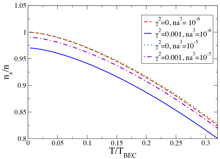
Figure 1: Plot of superfluid fraction in presence and absence of an uncorrelated disordered potential. The curve are derived from the two-fluid assumption $n=n_{s}+n_{n}$, with the normal contribution $n_{n}$ given by Eq. (52). The temperatures are in units of $T_{\text{BEC}}=2\pi\hbar^{2}n^{2/3}/(mk_{B}\zeta(3/2)^{2/3})$, i.e. the condensation temperature of an ideal Bose gas. The solid blue line and the dot-dashed violet one represent the behaviour of $n_{s}/n$ in presence of a disordered potential with $\gamma^{2}=0.001$ for two different values of the gas parameter $na_{s}^{3}=10^{-6}$ and $10^{-5}$ respectively. For the same values of $na_{s}^{3}$, the dashed red line and the dotted green correspond the case where there is no disorder contribution ($\gamma^{2}=0$).

In order to understand the relevance of Eq. (52), one has to remember that, in the pure system (i.e. $\gamma=0$), all the particles belong to the superflow. On the contrary, a disorder potential induce a superfluid depletion also at $T=0$ and, in addition, the parameter $\gamma$ may act as knob to destroy the superflow since

$$n_{s}^{(0)}(n_{0})=n-\frac{4}{d}n_{\gamma}(n_{0})\;.$$ (53)

In a similar way to the condensate fraction, we are not allowed to expand $n_{s}/n$ in the limit $g\rightarrow 0$ because Eq. (37) is divergent in that regime. Obviously, the superfluid density can be computed from the two-fluid assumption $n=n_{s}+n_{n}$ where $n_{n}$ is given by Eq. (52).

In fig. 1 we report the behaviour of the superfluid fraction in presence of a disordered but uncorrelated external potential with $\gamma^{2}=0.001$ for two different values of the gas parameter $na_{s}^{3}$. In order to highlight the crucial contribution due to disorder, we also consider the case where $\gamma^{2}=0$. It is immediate to realize that in pure system ($\gamma^{2}=0$) the whole system is superfluid at $T=0$, while the presence of a disorder potential lowers the curves, since there is an additional depletion at $T=0$. It is also interesting to underline that the more dilute is the system, the more evident is the detachment from the pure system.

IV The replicated action for superfluid bosons

The previous section has been focused on the extension of usual field-theory techniques superfluid bosons subject to a random external confinement. Moreover, the whole calculation has been carried out in the quenched regime, where we effectively average over different microscopic realization of the system with a given disorder configuration.

We have already made clear that this is not the only viable strategy and that it does not handle physical realizations where, for instance, the disorder potential also has a thermal component. This means that, looking at Eq. (14), it is not clear in which order integration and differentiation have to be performed. In order to overcome this ambiguity, the replica trick represents one of the most ingenious strategy. It was first developed in the context of spin glasses anderson-1975 ; parisi-book ; parisi-review but, in the following, we are going to detail how it can be applied to describe the role of disorder in ultracold bosonic gases.

Let us begin by considering again Eq. (14). The following three hypothesis represent the starting of the replica formalism. Thus,

• We assume that $\mathscr{Z}[J=0]=1$, establishing a proper normalization and implying that Eq. (14) has no dependence on $V_{\text{D}}$ in the denominator;

• it holds $\braket{\mathscr{O}}_{\text{th+dis}}=-\delta\braket{\log\mathscr{Z}}_{\text{dis}}/\delta_{J}|_{J=0}$;

• for $J\neq 0$ the partition function retains its algebraic properties.

Actually, the last point is a somewhat obscure way to state that the average procedure involves functionals linear in the disorder potential, since $V_{\text{D}}$ has been linearly added to the action. The great advantage provided by the replica trick can be understood from the formal relations reported below,

$$\log\mathscr{Z}[J]=\lim_{R\rightarrow 0}\frac{e^{R\log\mathscr{Z}}-1}{R}=\lim_{R\rightarrow 0}\frac{\mathscr{Z}^{R}-1}{R}$$ (54)

with $R\in\mathbb{N}$. The replacement of $\log\mathscr{Z}$ with an algebraic function of $\mathscr{Z}$ strongly reduces the complexity. Indeed, concerning the calculation of the expectation values, we have

$$\braket{\mathscr{O}}_{\text{th+dis}}=-\lim_{R\rightarrow 0}\frac{\delta}{\delta J}\frac{\mathscr{Z}^{R}}{R}\;.$$ (55)

Actually, within the replicated formalism, expectation values can be obtained by simply considering $R$ identical copies of the system under consideration. Concerning the functional integration, it does not alter the linear dependence of the action on the disorder field, because $[\exp(\int dV_{\text{D}})]^{R}=\exp(\sum^{R}\int dV_{\text{D}})$. Unfortunately all this comes with a price. Looking at Eq. (55) we realize that, at the end, we should perform an analytical continuation $R\rightarrow 0$. The point is that there is no guarantee at all that the function $\delta_{J}\braket{\mathscr{Z}^{R}}_{\text{dis}}$ is analytic all the way down to $R=0$ altland-book . This means that, from a mathematical standpoint, the replica trick is not a well-founded technique. Surprisingly, it is also true that it seems to rarely fail, at least when the disorder can be treated in a perturbative way parisi-book ; parisi-review .

Let us consider in the following the generalization of Eq. (10), namely given by

$$\tilde{\mathsf{P}}[U_{\text{D}}]=\exp\bigg{\{}-\frac{1}{2}\int_{0}^{\beta\hbar}d\tau\int d^{d}\mathbf{r}\;\gamma^{-2}(\mathbf{r},\tau)U_{\text{D}}^{2}(\mathbf{r},\tau)\bigg{\}}$$ (56)

where, actually, the disorder is assumed translationally invariant in time and space. In order to implement the replica trick within the context of superfluid bosonic systems, as an alternative to Eq. (19) we move to the phase-density representation, where

$$\psi(\mathbf{r},\tau)=\sqrt{n_{0}+\pi(\mathbf{r},\tau)}\;e^{i\varphi(\mathbf{r},\tau)}\;.$$ (57)

with $n_{0}=\psi_{0}^{2}$, $\psi_{0}^{2}$ being given by Eq. (18). From the equation above we deduce that $n(\mathbf{r},\tau)=n_{0}+\pi(\mathbf{r},\tau)$ and a perturbative strategy is easily implemented by assuming the smallness of density fluctuation. Thus, Eq. (57) becomes

$$\psi(\mathbf{r},\tau)\simeq\sqrt{n_{0}}\bigg{[}1+\frac{\pi(\mathbf{r},\tau)}{2n_{0}}\bigg{]}e^{i\varphi(\mathbf{r},\tau)}\;.$$ (58)

In order to understand the limitations of our approach, it is crucial to recall that $\braket{n(\mathbf{r},\tau)}_{\text{th}}=\braket{}{\psi(\mathbf{r},\tau)}{{}^{2}}_{\text{th}}$, while we often set $n\simeq n_{0}$ with $n_{0}=\big{|}\braket{\psi(\mathbf{r},\tau)}_{\text{th}}\big{|}^{2}$. Up to the Gaussian level this is an acceptable approximation since $\braket{\pi(\mathbf{r},\tau)}_{\text{th}}\simeq 0$. In the regime of small fluctuations, we can expand the mean-field analysis by retaining only the quadratic terms in $\pi(\mathbf{r},\tau)$ and $\varphi(\mathbf{r},\tau)$. The change of variables $\{\psi,\psi^{*}\}\rightarrow\{\pi,\varphi\}$ has a constant Jacobian determinant, therefore Eq. (3) reads

$$\mathscr{Z}\simeq\int\mathscr{D}[\pi,\varphi]\exp\bigg{\{}-\frac{1}{\hbar}S_{g}[\pi,\varphi]\bigg{\}}$$ (59)

with the periodic boundary conditions $\pi(\mathbf{r},\beta\hbar)=\pi(\mathbf{r},0)$ and $\varphi(\mathbf{r},\beta\hbar)=\varphi(\mathbf{r},0)$. The smallness of fluctuations allows to extend the integration range of the phase variable from $[-\pi,+\pi]$ to $[-\infty,+\infty]$. This decompactification has obviously to be addressed with particular attention when dealing with $d\leq 2$, where the enhancement of fluctuations prevents the occurring of a true long-range order and a more refined analysis is required altland-book ; mermin-1966 ; hohenberg-1967 ; villain-1975 ; kadanoff-1977 . The Gaussian action in Eq. (59) is given by

$$S_{g}[\pi,\varphi] =\int_{0}^{\beta\hbar}d\tau\int d^{d}\mathbf{r}\bigg{[}i\hbar\pi\frac{\partial\varphi}{\partial\tau}+\frac{n_{0}\hbar^{2}(\nabla\varphi)^{2}}{2m}+\frac{\hbar^{2}(\nabla\pi)^{2}}{8mn_{0}}-U_{\text{D}}(\mathbf{r},\tau)(n_{0}+\pi)$$ (60)

$$\qquad\qquad+\frac{1}{2}\int d^{d}\mathbf{r}^{\prime}\pi(\mathbf{r}^{\prime},\tau)V(|\mathbf{r}-\mathbf{r}^{\prime}|)\pi(\mathbf{r},\tau)\bigg{]}-\frac{1}{2}\beta\hbar L^{d}\tilde{V}(0)n_{0}^{2}$$

where we have imposed Eq. (18) to eliminate the dependence on the chemical potential and $U_{\text{D}}$ is distributed according to Eq. (56). The pertubative expansion up to the terms contained in Eq. (60) is equivalent to a one-loop expansion within a diagrammatic representation. Equivalently, in the second-quantization formalism this corresponds to the Bogoliubov approximation andersen-2004 .

The implementation of the replica trick requires the calculation of $\braket{\mathscr{Z}^{R}}_{\text{dis}}$. The (not-averaged) partition function is simply

$$\mathscr{Z}^{R}=\int\mathscr{D}[\pi,\varphi]\exp\bigg{\{}-\frac{1}{\hbar}\sum_{\alpha=1}^{R}S_{g}[\pi_{\alpha},\varphi_{\alpha}]\bigg{\}}\;,$$ (61)

where $S_{g}[\pi_{\alpha},\varphi_{\alpha}]$ is provided by Eq. (60) and $\mathscr{D}[\pi,\varphi]=\prod_{\alpha=1}^{R}\mathscr{D}[\pi_{\alpha},\varphi_{\alpha}]$. In case of a Gaussian disorder obeying to Eq. (56), Eq. (6) reads

$$\braket{\mathscr{Z}^{R}}_{\text{dis}} =\int\mathscr{D}[\pi,\varphi]\exp\bigg{\{}-\frac{1}{\hbar}\sum_{\alpha=1}^{R}S^{\text{(pure)}}_{g}[\pi_{\alpha},\varphi_{\alpha}]\bigg{\}}\times$$ (62)

$$\times\underbrace{\int\mathscr{D}[U_{\text{D}}]\exp\bigg{\{}-\frac{1}{2}\int_{0}^{\beta\hbar}d\tau\int d^{d}\mathbf{r}\;\gamma^{-2}(\mathbf{r},\tau)\,U_{\text{D}}^{2}(\mathbf{r},\tau)\bigg{\}}\exp\bigg{\{}-\frac{1}{\hbar}\sum_{\alpha=1}^{R}S^{\text{(coup)}}_{g}[U_{\text{D}},\pi_{\alpha}]\bigg{\}}}_{{}=(\star)}$$

where $S^{\text{(pure)}}_{g}[\pi_{\alpha},\varphi_{\alpha}]$ is Eq. (60) with $U_{\text{D}}=0$ and $S^{\text{(coup)}}_{g}[U_{\text{D}},\pi_{\alpha}]$ is given by

$$S^{\text{(coup)}}_{g}[U_{\text{D}},\pi_{\alpha}]=\int_{0}^{\beta\hbar}d\tau\int d^{d}\mathbf{r}\;U_{\text{D}}(\mathbf{r},\tau)\sum_{\alpha=1}^{R}\pi_{\alpha}(\mathbf{r},\tau)\;.$$ (63)

The second line of Eq. (62) is a Gaussian integral in $U_{\text{D}}$ such that

$$(\star)=\exp\bigg{\{}\frac{1}{2\hbar}\int_{0}^{\beta\hbar}d\tau\int d^{d}\mathbf{r}\;\gamma^{2}(\mathbf{r},\tau)\sum_{\alpha,\beta}\pi_{\alpha}(\mathbf{r},\tau)\pi_{\beta}(\mathbf{r},\tau)\bigg{\}}\;.$$ (64)

In this way, the replicated partition in Eq. (62) results in

$$\braket{\mathscr{Z}^{R}}_{\text{dis}}=\int\mathscr{D}[\pi,\varphi]\exp\bigg{\{}-\frac{1}{\hbar}\sum_{\alpha=1}^{R}S_{g}^{\text{(pure)}}[\pi_{\alpha},\varphi_{\alpha}]-\frac{1}{\hbar}\sum_{\alpha,\beta=1}^{R}S_{g}^{\text{(dis)}}[\pi_{\alpha},\pi_{\beta},\varphi_{\alpha},\varphi_{\beta}]\bigg{\}}\;.$$ (65)

For the sake of clarity we report below $S_{g}^{\text{(pure)}}$ and $S_{g}^{\text{(dis)}}$, namely

$$S_{g}^{\text{(pure)}}[\pi_{\alpha},\varphi_{\alpha}]=\int d^{d+1}\mathbf{s}\bigg{[}i\hbar\pi_{\alpha}\partial_{\tau}\varphi_{\alpha}+\frac{n_{0}\,\hbar^{2}(\nabla\varphi_{\alpha})^{2}}{2m}+\frac{\hbar^{2}(\nabla\pi_{\alpha})^{2}}{8mn_{0}}+\frac{1}{2}\int d^{d}\mathbf{r}^{\prime}\pi(\mathbf{r}^{\prime},\tau)V(|\mathbf{r}-\mathbf{r}^{\prime}|)\pi(\mathbf{r},\tau)\bigg{]}$$ (66)

$$S_{g}^{\text{(dis)}}[\pi_{\alpha},\pi_{\beta},\varphi_{\alpha},\varphi_{\beta}]=-\frac{1}{2}\int d^{d+1}\mathbf{s}\,\gamma^{2}(\mathbf{r},\tau)\pi_{\alpha}(\mathbf{s})\pi_{\beta}(\mathbf{s})$$ (67)

with $\mathbf{s}=(\mathbf{r},\tau)$. It is crucial to underline the relevance of Eq. (65). Indeed, it shows that also in presence of the simplest disorder potential ($\delta$-correlated both in time and space), the outlined formalism generates an effective quartic interaction between different replica indices. This fact can be understood by recalling the physical meaning of Feynman’s path. Despite its complexity, and indifferent to different replicas, the path integrals prefer to evolve towards the lowest possible potential. In other words they have a tendency to populate the same regions of the energy landscape.

Moving to the calculation of expectation values, the replicated formalism replaces the logarithm of the partition function with, basically, Eq. (65), where the Euclidean action of Eq. (60) is splitted into Eq. (66) and Eq. (67). According to Eq. (55), the joint thermal and disorder average is obtained through

$$\braket{{\,\mathscr{O}\,}}_{\text{th+dis}}=-\lim_{R\rightarrow 0}\frac{\delta}{\delta J}\frac{1}{R}\mathscr{Z}^{R}[J]=\lim_{R\rightarrow 0}\frac{1}{R}\braket{\,\mathscr{O}[\psi_{\alpha},\psi^{*}_{\alpha}]\,}_{\text{rep}}$$ (68)

where $\braket{\bullet}_{\text{rep}}$ has to be intended as a thermal average over the replicated partition function in Eq. (65) or, equivalently, over the action given by the sum of Eq. (66) and Eq. (67), i.e.

$$\braket{\,\mathscr{O}\,}_{\text{rep}}=\dfrac{\int\mathscr{D}[\pi,\varphi]\mathscr{O}\exp\{\hbar^{-1}(S_{g}^{\text{(pure)}}[\pi,\varphi]+S_{g}^{\text{(dis)}}[\pi,\varphi])\}}{\int\mathscr{D}[\pi,\varphi]\exp\{\hbar^{-1}(S_{g}^{\text{(pure)}}[\pi,\varphi]+S_{g}^{\text{(dis)}}[\pi,\varphi])\}}\;.$$ (69)

It is useful to expande the fields in Fourier series such that Eq. (66) reads

$$S_{g}^{\text{(pure)}}[\pi_{\alpha},\varphi_{\alpha}]=\frac{1}{2\beta\hbar L^{d}}\sum_{\mathbf{q}}\sum_{n}\chi_{\alpha}^{T}(-\mathbf{q},-\omega_{n})\mathscr{M}^{-1}(\mathbf{q},\omega_{n})\chi_{\alpha}(\mathbf{q},\omega_{n})$$ (70)

where we have defined the vector $\chi_{\alpha}$ as $\chi_{\alpha}(\mathbf{q},\omega_{n})^{T}\equiv\big{(}\varphi_{\alpha}(\mathbf{q},\omega_{n});\pi_{\alpha}(\mathbf{q},\omega_{n})\big{)}$ The pure inverse propagator in Eq. (70) is given by

$$\mathscr{M}^{-1}(\mathbf{q},\omega_{n})=\begin{pmatrix}n_{0}\dfrac{\hbar^{2}q^{2}}{m}&&-\hbar\omega_{n}\\ +\hbar\omega_{n}&&\dfrac{\hbar^{2}q^{2}}{4mn_{0}}+\tilde{V}(\mathbf{q})\end{pmatrix}\;.$$ (71)

On the other hand, for Eq. (63) we have now

$$S_{g}^{\text{(dis)}}[\pi_{\alpha},\pi_{\beta},\varphi_{\alpha},\varphi_{\beta}]=-\frac{1}{2\beta\hbar L^{d}}\sum_{\mathbf{q}}\sum_{n}\gamma^{2}(\mathbf{q},\omega_{n})\pi_{\alpha}^{*}(\mathbf{q},\omega_{n})\pi_{\beta}(\mathbf{q},\omega_{n})\;.$$ (72)

The equation above can be decomposed in its diagonal and off-diagonal contributions, leading us to the final equation for the Euclidean action of Gaussian fluctuations. By renaming $Q=(\mathbf{q},\omega_{n})$ and using the fact that $x(-Q)=x^{*}(Q)$, we have

$$S_{g}^{\text{(rep)}}[\pi,\varphi]=\frac{1}{2\beta\hbar L^{d}}\sum_{Q}\mathsf{X}^{\dagger}(Q)\mathbb{M}^{-1}(Q)\mathsf{X}(Q)\;.$$ (73)

In the equation above, the sum over the replicas is encoded in the $(R\times 2)$-dimensional column vector

$$\mathsf{X}(Q)=\begin{pmatrix}\chi_{1}(Q)\\ \chi_{2}(Q)\\ \vdots\\ \chi_{R}(Q)\end{pmatrix}\;.$$ (74)

The $R\times 2$ matrix $\mathbb{M}^{-1}(Q)$ in Eq. (73) is built as

$$\mathbb{M}^{-1}(Q)=\begin{pmatrix}\tilde{\mathscr{M}}^{-1}(Q)&\mathbb{B}(\gamma)&\dots&\dots&\mathbb{B}(\gamma)\\ \mathbb{B}(\gamma)&\tilde{\mathscr{M}}^{-1}(Q)&\dots&\dots&\mathbb{B}(\gamma)\\ \vdots&\vdots&\ddots&&\vdots\\ \vdots&\vdots&&\ddots&\mathbb{B}(\gamma)\\ \mathbb{B}(\gamma)&\mathbb{B}(\gamma)&\dots&\mathbb{B}(\gamma)&\tilde{\mathscr{M}}^{-1}(Q)\end{pmatrix}$$ (75)

with the generating blocks

$$\tilde{\mathscr{M}}^{-1}(Q) =\begin{pmatrix}n_{0}\frac{\hbar^{2}q^{2}}{m}&&-\hbar\omega_{n}\\ +\hbar\omega_{n}&&\frac{\hbar^{2}q^{2}}{4mn_{0}}+\tilde{V}(\mathbf{q})-\gamma^{2}(\mathbf{q},\omega_{n})\end{pmatrix}$$ (76)

$$\mathbb{B}(\gamma) =\begin{pmatrix}0&0\\ 0&-\gamma^{2}(\mathbf{q},\omega_{n})\\ \end{pmatrix}\;.$$ (77)

V Correlations functions in the replicated formalism

As detailed in App. A, the matrix $\mathbb{M}$ in Eq. (75) is diagonalized by a well-known unitary transformation, reading

$$\tilde{\mathbb{M}}^{-1}(Q)=\text{diag}\big{\{}\tilde{\mathscr{M}}_{R}^{-1}(Q),\underbrace{\tilde{\mathscr{M}}^{-1}(Q),\ldots,\tilde{\mathscr{M}}^{-1}(Q)}_{R-1\quad\text{times}}\big{\}}$$ (78)

with

$$\mathbb{M}^{-1}_{R}(Q)=\begin{pmatrix}n_{0}\frac{\hbar^{2}q^{2}}{m}&&-\hbar\omega_{n}\\ +\hbar\omega_{n}&&\frac{\hbar^{2}q^{2}}{4mn_{0}}+\tilde{V}(\mathbf{q})-R\gamma^{2}(\mathbf{q},\omega_{n})\end{pmatrix}\;.$$ (79)

Up to this level of approximation, correlation functions are specified by the entries of the fluctuation propagator. For the pure system, by assuming translational invariance both in time and space, we have

$$\braket{\chi_{j}(\mathbf{q},\omega_{n})\chi_{k}(\mathbf{q}^{\prime},\omega_{n^{\prime}})}_{\text{th}}=\mathscr{M}_{jk}(\mathbf{q},\omega_{n})\delta(\mathbf{q}+\mathbf{q}^{\prime})\beta\hbar\delta_{n,-n^{\prime}}\;.$$ (80)

On the other hand, according to Eq. (68), the replicated formalism provides both the disorder and the thermal average at the same time. For instance, concerning the density-density correlation function, we have

$$\braket{\pi^{*}(\mathbf{q},\omega_{n})\pi(\mathbf{q}^{\prime},\omega_{n^{\prime}})}_{\text{dis+th}} =\lim_{R\rightarrow 0}\frac{1}{R}\sum_{\alpha=1}^{R}\braket{\pi_{\alpha}(\mathbf{q},\omega_{n})\pi_{\alpha}(\mathbf{q}^{\prime},\omega_{n^{\prime}})}_{S_{g}^{\text{(rep)}}}$$ (81)

$$=\lim_{R\rightarrow 0}\frac{1}{R}\bigg{[}(R-1)\frac{n_{0}\hbar^{3}q^{2}/m}{\hbar^{2}\omega_{n}^{2}+E_{q}^{2}}+\frac{n_{0}\hbar^{2}q^{2}/m}{\hbar^{2}\omega_{n}^{2}+E_{q}^{2}-R\gamma^{2}(\mathbf{q},\omega_{n})n_{0}\dfrac{\hbar^{2}q^{2}}{m}}\bigg{]}\delta(\mathbf{q}+\mathbf{q}^{\prime})\beta\hbar\delta_{n,-n^{\prime}}$$

$$=\bigg{[}\frac{n_{0}\hbar^{3}q^{2}/m}{\hbar^{2}\omega_{n}^{2}+E_{q}^{2}}+\gamma^{2}(\mathbf{q},\omega_{n})\frac{n_{0}\hbar^{2}q^{2}q^{\prime 2}/m}{\big{(}\hbar^{2}\omega_{n}^{2}+E_{q}^{2}\big{)}\big{(}\hbar^{2}\omega_{n^{\prime}}^{2}+E_{q^{\prime}}\big{)}}\bigg{]}\delta(\mathbf{q}+\mathbf{q}^{\prime})\beta\hbar\delta_{n,-n^{\prime}}$$

where the final result is obtained by expanding the second line up to the first order in $R$. Moreover, we have

$$E_{q}=\sqrt{\epsilon_{q}\big{[}\epsilon_{q}+2n_{0}\tilde{V}(\mathbf{q})\big{]}}\;,$$ (82)

nothing else than Eq. (29) with the saddle-point replacement $\mu=\tilde{V}(0)\,n_{0}$. The remaining correlations are computed in the same way, leading to

$$\braket{\varphi^{*}(\mathbf{q},\omega_{n})\varphi(\mathbf{q}^{\prime},\omega_{n^{\prime}})}_{\text{dis+th}} =\bigg{[}\frac{mE_{q}^{2}/(n_{0}\hbar q^{2})}{\hbar^{2}\omega_{n^{\prime}}^{2}+E_{q}^{2}}+\frac{\hbar^{2}\omega_{n}\omega_{n^{\prime}}}{\big{(}\hbar^{2}\omega_{n}^{2}+E_{q}^{2}\big{)}\big{(}\hbar^{2}\omega_{n^{\prime}}^{2}+E_{q^{\prime}}\big{)}}\gamma^{2}(\mathbf{q},\omega_{n})\bigg{]}\delta(\mathbf{q}+\mathbf{q}^{\prime})\beta\hbar\delta_{n,-n^{\prime}}$$ (83)

$$\braket{\varphi^{*}(\mathbf{q},\omega_{n})\pi(\mathbf{q}^{\prime},\omega_{n^{\prime}})}_{\text{dis+th}} =\bigg{[}\frac{\hbar^{2}\omega_{n}}{\hbar^{2}\omega_{n}^{2}+E_{q}^{2}}+\frac{n_{0}\hbar^{3}q^{\prime 2}\omega_{n^{\prime}}/m}{\big{(}\hbar^{2}\omega_{n}^{2}+E_{q}^{2}\big{)}\big{(}\hbar^{2}\omega_{n^{\prime}}^{2}+E_{q^{\prime}}\big{)}}\gamma^{2}(\mathbf{q},\omega_{n})\bigg{]}\delta(\mathbf{q}+\mathbf{q}^{\prime})\beta\hbar\delta_{n,-n^{\prime}}$$

Besides the phase and density correlators, one of the most important correlation functions is the current one, defined as

$$\mathscr{C}_{ij}(\mathbf{r},\tau;\mathbf{r}^{\prime},\tau^{\prime})=m^{-1}\big{[}\braket{g_{i}(\mathbf{r},\tau)g_{j}(\mathbf{r}^{\prime},\tau^{\prime})}-\braket{g_{i}(\mathbf{r},\tau)}\braket{g_{j}(\mathbf{r}^{\prime},\tau^{\prime})}\big{]}\;,$$ (84)

where the notation $\braket{\ldots}$ represents, for now, a general average procedure. In the phase-density representation, from Eq. (57) it is easy to verify that the current density $\mathbf{g}=\hbar(n_{0}+\pi)\nabla\varphi/m$. Thus, by making use of the Wick theorem fetter-book to disentagle the four-field correlator in Eq. (84), in the Fourier space one obtains tauber-1997

$$\mathscr{C}_{ij}(\mathbf{q},\omega_{n};\mathbf{q}^{\prime},\omega_{n^{\prime}}) =-\hbar^{2}mn_{0}^{2}q_{i}q_{j}\Braket{\varphi(\mathbf{q},\omega_{n})\varphi(\mathbf{q}^{\prime},\omega_{n^{\prime}})}+$$ (85)

$$-\frac{1}{(\beta L^{d})^{2}}\sum_{\mathbf{k},\omega_{m}}\sum_{\mathbf{k}^{\prime},\omega_{m^{\prime}}}k_{i}k^{\prime}_{j}\bigg{[}\Braket{\pi(\mathbf{q}-\mathbf{k},\omega_{l-m})\pi(\mathbf{q}^{\prime}-\mathbf{k}^{\prime},\omega_{l^{\prime}-m^{\prime}})}\Braket{\varphi(\mathbf{k},\omega_{m})\varphi(\mathbf{k}^{\prime},\omega_{m^{\prime}})}+$$

$$\qquad\qquad+\Braket{\pi(\mathbf{k}-\mathbf{q},\omega_{m-l})\varphi(\mathbf{k}^{\prime},\omega_{m^{\prime}})}\Braket{\pi(\mathbf{k}^{\prime}-\mathbf{q}^{\prime},\omega_{m^{\prime}-l^{\prime}})\varphi(\mathbf{k},\omega_{m})}\bigg{]}\;.$$

Thanks to the replica trick, the disorder contribution is taken into account by considering the correlators over the replicated Gaussian action, namely Eqs. (81) and (83).

The current response function in Eq. (85) is crucial since it encodes the superfluid character of the system. This point is clarified by noticing that $\mathscr{C}_{ij}$ is a 2-rank tensor, so it can be decomposed in its longitudinal and transverse components by means of the projectors $\mathscr{P}^{L}_{ij}=q_{i}q_{j}/q^{2}$ and $P^{T}_{ij}=\delta_{ij}-\mathscr{P}^{L}_{ij}$. It has been shown (see baym-1967 and ueda-book for a pedagogical review), that the static limit of transverse component of Eq. (85) $\mathscr{C}_{ij}^{T}(\mathbf{q},\omega_{n})\equiv(d-1)^{-1}\sum_{ij}\mathscr{P}_{ij}^{T}(\mathbf{q},\omega_{n})\mathscr{C}_{ij}(\mathbf{q},\omega_{n})/\hbar$ corresponds to the normal component of the system. By replacing the replicated correlator given by Eqs. (81) and (83) into Eq. (85), after burdensome (but standard) algebra, we find

$$n_{n} =\lim_{q\rightarrow 0}\braket{\mathscr{C}^{T}(\mathbf{q},0)}_{\text{th+dis}}$$ (86)

$$=\frac{1}{d\beta L^{d}}\sum_{\mathbf{k},\omega_{m}}\bigg{[}\bigg{(}\frac{\hbar^{2}k^{2}}{m}\bigg{)}\frac{E_{k}^{2}-\hbar^{2}\omega_{m}^{2}}{(\hbar^{2}\omega_{m}^{2}+E_{q}^{2})^{2}}+n_{0}\bigg{(}\frac{\hbar^{2}k^{2}}{m}\bigg{)}^{2}\frac{E_{k}^{2}-3\hbar^{2}\omega_{m}^{2}}{(\hbar^{2}\omega_{m}^{2}+E_{k}^{2})^{3}}\gamma^{2}(\mathbf{k},\omega_{m})\bigg{]}\;.$$

When the time scale of the disorder potential is frozen, i.e. for

$$\gamma^{2}(\mathbf{q},\omega_{n})=\gamma^{2}(\mathbf{q})\beta\delta_{n,0}\;,$$ (87)

Eq. (86) becomes

$$n_{n}(n_{0},T)=\frac{\beta}{d}\int\frac{d^{d}\mathbf{q}}{(2\pi)^{d}}\frac{\hbar^{2}q^{2}}{m}\frac{e^{\beta E_{q}}}{(e^{\beta E_{q}}-1)^{2}}+\frac{4n_{0}}{d}\int\frac{d^{d}\mathbf{q}}{(2\pi)^{d}}\bigg{(}\frac{\hbar^{2}q^{2}}{2m}\bigg{)}^{2}\frac{\gamma^{2}(\mathbf{q})}{E_{q}^{4}}\;.$$ (88)

With the further simplification of a constant disorder correlator $\gamma^{2}$, the equation above equates to Eq. (52). So, Eq. (88) reduces corretly to the quenched disorder regime and agrees with results reported in tauber-1997 ; schakel-1997 ; giorgini-1994 .

In order to compute the condensate depletion through the replicated correlators in Eqs. (81) and (83), we rely upon the equation fetter-book

$$n=n_{0}+\frac{1}{\beta\hbar}\int\frac{d^{d}\mathbf{q}}{(2\pi)^{d}}\sum_{n}\,e^{i\omega_{n}0^{+}}\big{[}\braket{\psi(\mathbf{r},\tau)\psi^{*}(\mathbf{r}^{\prime},\tau^{\prime})}-n_{0}\big{]}\;.$$ (89)

Following the phase-density representation in Eq. (57), we expand the fields $\psi$ and $\psi^{*}$ up to the linear order in the fluctuations $\psi(\mathbf{r},\tau)\simeq\sqrt{n_{0}}[1+\pi(\mathbf{r},\tau)/(2n_{0})+i\varphi(\mathbf{r},\tau)]$, such that the resulting correlators in Eq. (89) are Gaussian. In the Fourier space we have

$$\braket{\psi(\mathbf{q},\omega_{n})\psi^{*}(\mathbf{q}^{\prime},\omega_{n^{\prime}})}-n_{0}\simeq\frac{1}{4n_{0}}\braket{\pi\pi^{\prime}}-\frac{i}{2}\braket{\pi\varphi^{\prime}}+\frac{i}{2}\braket{\varphi\pi^{\prime}}+n_{0}\braket{\varphi\varphi^{\prime}}$$ (90)

where the prime signal the dependence on $Q^{\prime}=(\mathbf{q}^{\prime},\tau^{\prime})$ and, similarly to Eq. (84), $\braket{\ldots}$ corresponds to a general average procedure. In order to include the disorder contribution one simply has to consider the replicated correlators in Eqs. (81) and (83), where space-time translational invariance restored by assuming Eq. (80).

We then have

$$n =n_{0}+\int\frac{d^{d}\mathbf{q}}{(2\pi)^{d}}\bigg{[}\frac{\epsilon_{q}+n_{0}\tilde{V}(q)}{2E_{q}}-\frac{1}{2}+\frac{\epsilon_{q}+n_{0}\tilde{V}(q)}{E_{q}}\bigg{(}\frac{1}{e^{\beta E_{q}}-1}\bigg{)}$$ (91)

$$\qquad\qquad\qquad\qquad+\frac{n_{0}}{\beta\hbar}\sum_{m}\frac{\epsilon_{q}^{2}-\hbar^{2}\omega_{m}}{(\hbar^{2}\omega_{m}^{2}+E_{q}^{2})^{2}}\gamma^{2}(\mathbf{q},\omega_{m})\bigg{]}\;.$$

The first line represents the contribution coming from the pure system, reading Eq. (40) at $T=0K$. On the other hand, the second line accounts for the disorder contribution. For a point-like frozen disorder as in Eq. (87), one can verify that

$$n_{\gamma}(n_{0})=n_{0}\int\frac{d^{d}\mathbf{q}}{(2\pi)^{d}}\bigg{(}\frac{\hbar^{2}q^{2}}{2m}\bigg{)}^{2}\,\frac{\gamma^{2}(\mathbf{q})}{E_{q}^{4}}$$ (92)

By comparing the equation above and Eq. (88), at zero-temperature the disorder contribution to the condensate depletion and the normal component of the system are deeply related, namely

$$n_{\gamma}(n_{0})=\frac{d}{4}n_{n}(n_{0},T=0)$$ (93)

VI Conclusions and future perspectives

In this review, we have reviewed the crucial aspects of a field-theory approach to superfluid bosons moving in a random environment. Within the powerful framework of functional integration, we have recovered the important result on the superfluid and condensate depletion in presence of an external disorder huang-1992 ; giorgini-1994 ; schakel-1997 . Moreover, we have shown how the theoretical description can be generalized beyond the assumption of a static external disorder by using the replicated formalism navez-2007 . Obviously, our pedagogical overview has to left out other interesting and crucial issues. For instance, we have pointed out in Sec. III that our perturbative approach lacks self-consistency, since we are expanding above a uniform background also in presence of an external potential. In order to overcome this point, in khellil-2016 ; khellil-2016-2 the authors present a self-consistent implementation relying upon the Hartee-Fock mean-field theory within the replica formalism. Moreover, our review does not include any discussion about the eventual occuring of the superfluid-glass transition in three or lower dimensions. This is a crucial topic, deserving a separate investigation. Numerical simulations based on quantum Monte Carlo methods are likewise important, since they are ab-initio calculation and may shed light on unexpected effects. For instance, in giorgini-2002 the non-trivial relation between superfluidity and condensation is numerically investigated, while in ng-2015 the worm algorithm provides an estimation for critical exponents of the superfluid-glass transition in two-dimensions.

Another promising line of research concerns the possibility that disorder does not always act in a parasitic way, generating, on the contrary, surprising dynamical effects. In the context of condensed matter theory, one of the most striking example is given by the quantum Hall transition pruisken-1987 , where impurity scattering plays a crucial role. On the other hand, very recently it was shown that a certain degree of random fluctuations, such as thermal noise, may enhance the transport properties of a particles ensemble. While Anderson localization anderson-1959 acts to halt the flow of a certain quantity, in caruso-2015 ; potocnik-2018 the authors observe a boosting of transport through optical fibers and superconducting circuits. The reason is the so-called environment-assisted quantum trasport, which relies crucially upon the presence of a certain degree of disorder. Indeed, while the coherence of the system is reduced by propagating in a disordered medium, this also reduces the possibility of destructive interference responsible for Anderson localization.

This phenomenon can pave the way to novel interesting protocol to engineer more efficient quantum devices, by tuning the coupling with the environment to enhance the trasport of a desired quantity. Recent experimental confirmations have been produced by using a one-dimensional array of trapped ions maier-2019 . Thus, it would be extremely interesting to review to effect in the context of ultracold atoms, both from an experimental and theoretical point of view.

Acknowlegdements

LS acknowledges for partial support the FFABR grant of Italian Ministry of Education, University and Research. AC thanks Andrea Tononi for useful discussions and meaningful insight on the manuscript.

Appendix A Diagonalization of a block circulant matrix

It is possible to perform a block diagonalization of $\mathbb{M}^{-1}$ in Eq. (75) by noticing its circulant structure. Indeed, $\mathbb{G}^{-1}$ is generated by cyclically permuting the elements (in this case $2\times 2$ matrices) of its first row. In this sense, we can formally write down

$$\mathbb{M}^{-1}(Q)=\text{Circ}\big{\{}\tilde{\mathscr{M}}^{-1}(Q),\underbrace{\mathbb{B}(Q),\ldots,\mathbb{B}(Q)}_{{}\text{$R-1$ times}}\big{\}}\;.$$ (94)

It has been shown davis-book ; olson-2014 that, given $R$ the number of the generating matrices and $M$ their dimension, every block circulant matrix $\mathbb{A}$ is block diagonalized by the same unitary transformation. Indeed, one can verify that

$$(\mathbb{E}_{R}^{\dagger}\otimes 1_{M})\mathbb{A}(\mathbb{E}_{R}\otimes 1_{M})=\text{diag}\{\Lambda_{1},\ldots,\Lambda_{R}\}$$ (95)

where the $\Lambda_{j}$ are the $2\times 2$ eigenblocks, specified by $\Lambda_{j}=\mathscr{M}^{-1}+\sum_{\alpha=1}^{R-1}\mathbb{B}\;w_{R}^{\alpha j}$. The $\otimes$ symbol denotes the direct product of the two matrices. In Eq. (95) the key ingredient is the Fourier matrix, defined as

$$\mathbb{E}_{R}=\frac{1}{\sqrt{R}}\begin{pmatrix}1&1&1&\dots&\dots&1\\ 1&w_{R}&w_{R}^{2}&\dots&\dots&w_{R}^{R-1}\\ 1&w_{R}^{2}&w_{R}^{4}&\dots&\dots&w_{R}^{2(R-1)}\\ \vdots&\vdots&\vdots&\ddots&&\vdots\\ \vdots&\vdots&\vdots&&\ddots&\vdots\\ 1&w_{R}^{R-1}&w_{R}^{2(R-1)}&\dots&\dots&w_{R}^{(R-1)^{2}}\\ \end{pmatrix}$$ (96)

with $w_{R}=\exp(2\pi i/R)$ the fundamental root of the unity.

References

• (1) M. H. Anderson, J. R. Ensher, M. R. Matthews, C. E. Wieman and E. A. Cornell, Observation of Bose-Einstein Condensation in a Dilute Atomic Vapor, Science 269, 5221 (1995).
• (2) K. B. Davis et al., Bose-Einstein Condensation in a Gas of Sodium Atoms, Phys. Rev. Lett. 75, 3969 (1995).
• (3) C. J. Pethick and H. Smith, Bose-Einstein Condensation in Dilute Gases, (Cambridge Univ. Press, 2011).
• (4) T. Langen, R. Geiger and J. Schmiedmayer, Ultracold atoms out of equilibrium, Annu. Rev. Condens. Matt. Phys. 6, 201-17 (2015).
• (5) M. P. A. Fisher, P. B. Weichman, G. Grinstein and D. S. Fisher, Boson localization and the superfluid-insulator transition, Phys. Rev. B. 40, 546 (1989).
• (6) M. Greiner, O. Mandel, T. Esslinger, T. W. Hänsch and I. Bloch, Quantum phase transition from a superfluid to a Mott insulator in a gas of ultracold atoms, Nature 415, 39-44 (2002).
• (7) T. Giamarchi, Quantum Physics in One Dimensions, (Clarendon Press, Oxford, 2003).
• (8) Z. Hadzibabic and J. Dalibard, Two-dimensional Bose fluids: an atomic physics perspective, Rivista del Nuovo Cimento 34, 389 (2011).
• (9) B. Paredes, A. Widera, V. Murg, O. Mandel, S. Folling, I. Cirac, G. V. Shlyapnikov, T. W. Hänsch, and I. Bloch, Tonks–Girardeau gas of ultracold atoms in an optical lattice, Nature (London) 429, 277 (2004).
• (10) T. Kinoshita, T. Wenger, and D. S. Weiss, Observation of a One-Dimensional Tonks-Girardeau Gas Science 305, 1125 (2004).
• (11) Z. Hadzibabic, P. Krüger, M. Cheneau, B. Battelier and J. Dalibard, Berezinskii-Kosterlitz- ouless crossover in a trapped atomic gas, Nature 441, 1118 (2006).
• (12) V. Schweikhard, S. Tung and E. A. Cornell, Vortex proliferation in the Berezinskii-Kosterlitz- ouless regime on a two-dimensional lattice of Bose-Einstein condensates, Phys. Rev. Lett. 99, 030401 (2007).
• (13) C. Neuenhahn and F. Marquardt, Quantum simulation of expanding space–time with tunnel-coupled condensates, New J. Phys. 17, 125007 (2015).
• (14) O. Fialko, B. Opanchuk, A. I. Sidorov, P. D. Drummond and J. Brand, The universe on a table top: engineering quantum decay of a relativistic scalar field from a metastable vacuum, J. Phys. B: At. Mol. Opt. Phys. 50, 024003 (2017).
• (15) J. Braden, M. C. Johnson, H. V. Peiris and S. Weinfurtner, Towards the cold atoms analog of the false vacuum, J. High En. Phys. 2018:14 (2018).
• (16) S. Liberati, M. Visser and S. Weinfurtner, Analogue quantum gravity phenomenology from a two-component Bose-Einstein condensate, Class. Quant. Grav. 23, 3129 (2006).
• (17) D. M. Kurkcuoglu and C. Sá de Melo, Unconventional color superfluidity in ultra-cold fermions: Quintuplet pairing, quintuple point and pentacriticality, arXiv:1811.07272 (2018).
• (18) A. Kamenev, Many-body theory of non-equilibrium systems, in Nanophysics: Coherence and Transport, p. 177-246 (Elsevier, Amsterdam, 2005).
• (19) M. Ma and P. A. Lee, Localized superconductors, Phys. Rev. B 32, 5658 (1985).
• (20) M. Ma, B. I. Halpering and P. A. Lee, Strongly disordered superfluids: Quantum fluctuations and critical behavior, Phys. Rev. B 34, 3136 (1986)
• (21) P. W. Anderson, Absence of diffusion in certain random lattices, Phys. Rev. 109, 1492 (1959).
• (22) B. Damski, J. Zakrzewski, L. Santos, P. Zoller and M. Lewenstein, Atomic Bose and Anderson Glasses in Optical Lattices, Phys. Rev. Lett. 91, 080403 (2003).
• (23) T. Schulte, S. Drenkelforth, J. Kruse, W. Ertmer, J. Arlt, K. Sacha, J. Zakrzewski and M. Lewenstein, Routes Towards Anderson-Like Localization of Bose-Einstein Condensates in Disordered Optical Lattices, Phys. Rev. Lett. 95, 170411 (2005).
• (24) J. Billy, V. Josse, Z. Zuo, A. Bernard, B. Hambrecht, P. Lugan, D. Clement, L. Sanchez-Palencia, P. Bouyer and A. Aspect, Direct Observation of Anderson Localization of Matter-Waves in a Controlled Disorder, Nature 453, 891 (2008).
• (25) G. Roati, C. D’Errico, L. Fallani, M. Fattori, C. Fort, M. Zaccanti, G. Modugno, M. Modugno and M. Inguscio, Anderson Localization of a Non-Interacting Bose-Einstein Condensate, Nature 453, 895 (2008).
• (26) J. C. Dainty, An introduction to Gaussian speckle, Proc. SPIE 243, 2 (1980).
• (27) J. W. Goodman, Speckle Phenomena in Optics: Theory and Applications, (Viva Books Private Limited, 2010).
• (28) J. E. Lye, L. Fallani, M. Modugno, D. S. Wiersma, C. Fort and M. Inguscio, A Bose-Einstein condensate in a random potential, Phys. Rev. Lett. 95, 070401 (2005).
• (29) D. Clément, A. F. Varón, M. Hugbart, J. A. Retter, P. Bouyer, L. Sanchez-Palencia, D. M. Gangardt, G. V. Shlyapnikov and A. Aspect, Suppression of Transport of an Interacting Elongated Bose-Einstein Condensate in a Random Potential, Phys. Rev. Lett. 95, 170409 (2005).
• (30) M. Ghabour and A. Pelster, Bogoliubov theory of dipolar Bose gas in a weak random potential, Phys. Rev. A 90, 063636 (2014).
• (31) H. T. C. Stoof, D. B. M. Dickerscheid and K. Gubbels, Ultracold Quantum Fields (Springer, Dordrecht, 2009).
• (32) L. Salasnich and F. Toigo, Zero-point energy of ultracold atoms, Phys. Rep. 640, 1-29 (2016).
• (33) K. Huang and H.-F. Meng, Hard-Sphere Bose Gas in Random External Potential, Phys. Rev. Lett. 69, 644 (1992).
• (34) S. Giorgini, L. Pitaevskii and S. Stringari, Effects of disorder in a dilute Bose gas Phys. Rev. B 49, 18 (1994).
• (35) U. Taüber and D. R. Nelson, Superfluid bosons and flux liquids: disorder, thermal fluctuations, and finite-size effects, Phys. Rep. 289, 157 (1997).
• (36) A. V. Lopatin and V. M. Vinokur, Thermodynamics of the Superfluid Dilute Bose Gas with Disorder, Phys. Rev. Lett. 88, 235503 (2002).
• (37) G. M. Falco, A. Pelster and R. Graham, Thermodynamics of a Bose-Einstein condensate with weak disorder Phys. Rev. A 75, 063619 (2007).
• (38) T. Giamarchi and H. J. Schulz, Anderson localization and interactions in one-dimensional metals, Phys. Rev. B 37, 325 (1988).
• (39) P. Navez, A. Pelster and R. Graham, Bose condensed gas in strong disorder potential with arbitrary correlation length, App. Phys. B 86, 395-398 (2007).
• (40) V. I. Yukalov andd R. Graham, Bose-Einstein condensed systems in random potentials, Phys. Rev. A 75, 023619 (2007).
• (41) G. M. Falco, T. Nattermann and V. L. Pokrovsky, Weakly interacting Bose gas in a random environment, Phys. Rev. B 80, 104515 (2009).
• (42) T. Khellil, A. Balaz and A. Pelster, Analytical and numerical study of dirty bosons in a quasi-one-dimensional harmonic trap, New J. Phys. 18, 063003 (2016).
• (43) T. Khellil and A. Pelster, Hartree-Fock Mean-Field Theory for Trapped Dirty Bosons, J. Stat. Mech. 063301 (2016).
• (44) A. Altland and B. Simons, Condensed Matter Field Theory (Cambridge University Press, 2010).
• (45) J. Hertz, Disordered Systems, Phys. Scr. 1985, 1 (1985).
• (46) D. R. Nelson and P. Le Doussal, Correlations in flux liquids with weak disorder, Phys. Rev. B 42, 16 (1990).
• (47) A. M. J. Schakel, Quantum critical behavior of disordered superfluids, Phys. Lett. A 224, 287 (1997).
• (48) T. C. Lubensky, Critical properties of the random-spin model from the $\epsilon$-expansion, Phys. Rev. B 11, 9 (1975).
• (49) G. Grinstein and A. Luther, Applications of the renormalization group to phase transition in disordered systems, Phys. Rev. B 13, 3 (1976).
• (50) A. M. J. Schakel, Boulevard of Broken Symmetries: Effective Field Theories of Condensed Matter, (World Scientific, Singapore, 2008).
• (51) G. E. Astrakharchik, J. Boronat, J. Casulleras, I. L. Kurbakov, and Yu. E. Lozovik, Equation of state of a weakly interacting two-dimensional Bose gas studied at zero temperature by means of quantum Monte Carlo methods, Phys. Rev. A 79, 051602 (2009).
• (52) A. Tononi, A. Cappellaro and L. Salasnich, Condensation and superfluidity of dilute Bose gases with finite-range interaction, New J. Phys. 20, 125007 (2018).
• (53) L. Salasnich, Nonuniversal Equation of State of the Two-Dimensional Bose Gas, Phys. Rev. Lett. 118, 130402 (2017).
• (54) A. Tononi, Zero-temperature equation of state of a two-dimensional bosonic quantum fluid with finite-range interaction, Condens. Matter 4(1), 20 (2019).
• (55) J. Wehr, A. Niederberger, L. Sanchez-Palencia and M. Lewenstein, Disorder versus the Mermin-Wagner-Hohenberg effect: From classical spin systems to ultracold atomic gases, Phys. Rev. B 74, 224448 (2006).
• (56) A. Boudjemaa and G.V. Shlyapnikov, Two-dimensional dipolar Bose gas with the roton-maxon excitation spectrum, Phys. Rev. A 87, 025601 (2013).
• (57) A. Boudjemaa, Two-dimensional dipolar bosons with weak disorder, Phys. Lett. A 379, 2484-2487 (2015).
• (58) L. D. Landau and E. M. Lifshitz, Statistical Physics 2, (Pergamon Press, Oxford, 1987).
• (59) I. M. Khalatnikov, An Introduction to the Theory of Superfluidity (Westwiew Press, Oxford, 2000).
• (60) M. E. Fisher, M. N. Barber and D. Jasnow, Helicity, Modulus, Superfluidity and Scaling in Isotropic Systems, Phys. Rev. A 8, 1111 (1973).
• (61) E. Taylor, A. Griffin, N. Fukushima and Y. Ohashi, Pairing fluctuations and the superfluid density through the BCS-BEC crossover, Phys. Rev. A 74, 063626 (2006)
• (62) S. F. Edwards and P. W. Anderson, Theory of spin glasses, J. Phys. F 5, 965-974 (1975).
• (63) M. Mezard, G. Parisi and M. Virasoro, Spin Glass Theory and Beyond: An Introduction to the Replica Method and Its Applications (World Scientific, 1987).
• (64) G. Parisi, Glasses, replicas and all that, in Les Houches - Ecole d’ été de Physique Théorique, Vol. 77 (Elsevier, 2004).
• (65) N. D. Mermin and H. Wagner, Absence of Ferromagnetism or antiferromagnetism in one- or two- dimensional isotropic heisenberg models, Phys. Rev. Lett. 17, 1133 (1966)
• (66) P. C. Hohenberg, Existence of Long-Range Order in One and Two Dimensions, Phys. Rev. 158, 383 (1967).
• (67) J. Villain, Theory of one- and two-dimensional magnets with an easy magnetization plane. II. The planar, classical, two-dimensional magnet, Journal de Physique 36, 581 (1975).
• (68) J. V. José, L. P. Kadanoff, S. Kirkpatrick and D. R. Nelson, Renormalization, vortices and symmetry-breaking perturbations in the two-dimensional planar model, Phys. Rev. B 16, 1217 (1977).
• (69) J. O. Andersen, Theory of the weakly interacting Bose gas, Rev. Mod. Phys. 76, 599 (2004).
• (70) A. L. Fetter and J. D. Walecka, Quantum Theory of Many-particle systems (Dover, 2003).
• (71) G. Baym, Microscopic Description of Superfluidity, in Mathematical Methods in Solid State and Superfluid Theory (Springer, 1967).
• (72) M. Ueda, Fundamentals and New Frontiers in Bose-Einstein Condensations, (World Scientific, 2010).
• (73) P. J. Davis, Circulant Matrices (Wiley, 2${}^{\text{nd}}$ ed., New York, 1979).
• (74) B. Olson, S. Shaw, C. Shi, C. Pierre and R. Parker, Circulant Matrices and Their Application to Vibration Analysis Applied Mechanics Review 66, 4 (2014).
• (75) G. E. Astrakharchik, J. Boronat, J. Casulleras and S. Giorgini, Superfluidity versus Bose-Einstein condensation in a Bose gas with disorder, Phys. Rev. A 66, 023603 (2002).
• (76) R. Ng and E. S. Sorensen, Quantum Critical Scaling of Dirty Bosons in Two Dimensions, Phys. Rev. Lett. 114, 255701 (2015).
• (77) A. M. M. Pruisken, Field theory, scaling and the localization problem in The Quantum Hall Effect (Springer-Verlag, 1987).
• (78) S. Viciani, M. Lima, M. Bellini and F. Caruso, Observation of noise-assisted transport in an all-optical cavity-based network, Phys. Rev. Lett. 115, 083601 (2015).
• (79) A. Potocnik et al., Studying light-harvesting models with superconducting circuits, Nature Commun. 9, 904 (2018).
• (80) C. Maier et al., Environment-Assisted Quantum Transport in a 10-qubit Network, Phys. Rev. Lett. 122, 050501 (2019).