First-Principles Determination of Electron-Ion Couplings
in the Warm Dense Matter Regime

Abstract

We present first-principles calculations of the rate of energy exchanges between electrons and ions in nonequilibrium warm dense plasmas, liquid metals and hot solids, a fundamental property for which various models offer diverging predictions. To this end, a Kubo relation for the electron-ion coupling parameter is introduced, which includes self-consistently the quantum, thermal, non-linear and strong coupling effects that coexist in materials at the confluence of solids and plasmas. Most importantly, like other Kubo relations widely used for calculating electronic conductivities, the expression can be evaluated using quantum molecular dynamics simulations. Results are presented and compared to experimental and theoretical predictions for representative materials of various electronic complexity, including aluminum, copper, iron and nickel.

The last decade has seen remarkable progress in our ability to form and interrogate in the laboratory materials under conditions at the confluence of solids and hot plasmas in the so-called warm dense matter regime Grazianietal2014 ; Frontierreport2017 . These experimental advances severely challenge our arsenal of theoretical techniques, simulation tools and analytical models. In addition to including the coexisting quantum, thermal, disorder and strong Coulomb interaction effects, theoretical approaches are needed that can also describe non-equilibrium conditions Ng_et_al_1995 ; Faustlin2010 ; Ng2012 ; Chen2013 ; Leguay2013 ; Clerouin2015 ; Zylstra2015 ; Cho_et_al_2015 ; Dorchies2016 ; Jourdain_et_al_2018 ; Ogitsu2018 ; Daligault_Dimonte_2009 . A particularly important property is the electron-ion coupling factor that measures the rate of energy exchanges between electrons and ions Ng2012 . Indeed, experiments typically produce transient, non-equilibrium conditions and measurements may be misleading if recorded while the plasma species are still out of equilibrium. Moreover, like the electron-phonon coupling, the electron-ion coupling may be a unique indicator of the underlying electronic structure and of the basic interaction processes occuring in the warm dense matter regime. Remarkably, while even for simple materials various models offer diverging predictions (see table 1), the electron-ion coupling factor is now accessible to experimental measurements thanks to the diagnostic capabilities offered by the new generation of x-ray light sources Leguay2013 ; Cho_et_al_2015 ; Dorchies2016 ; Jourdain_et_al_2018 ; Ogitsu2018 .

Here, we use a combination of first-principles theory and ab-initio molecular dynamics simulations to calculate the electron-ion coupling of materials under warm dense matter conditions. In the same way as with the now routine ab-initio calculations of electrical and thermal conductivities Desjarlais_et_al_2002 ; Holst2011 ; Sjostrom2015 , the approach offers a very useful comparison with the experimental measurements and a useful test of theories, it gives insight into the underlying physics, and it permits an extension into conditions not covered by the experiments. The electron-ion coupling is related to the friction coefficients felt by individual ions due to their non-adiabatic interactions with electrons. Each coefficient satisfies a Kubo relation given by the time integral of the autocorrelation function of the interaction force of an ion with the electrons, which is evaluated using density functional theory based quantum molecular dynamics simulations. In this Letter, we outline the underlying theory and present results for a set of relevant materials and physical conditions. Details of mathematical proofs and algorithms will be presented in an extended manuscript SimoniDaligault2019 . Below, $\hbar$ is the reduced Planck constant, $k_{B}$ is the Boltzmann constant.

Theoretical model	$G_{ei}$ $(10^{17}\,{\rm W/m^{3}K)}$
Spitzer-Brysk	$160$ Brysk1975
Fermi golden rule	$5$ Hazak2001 ; Daligault_Mozyrsky_2008
Coupled modes	$0.33$ DharmaWardana2001 ; $0.1$ Vorberger2012
Electron-phonon	$2.6$ Lin_et_al_2008 ; $5$ Waldecker2016

Table 1: Electron-ion coupling for solid density aluminum at melting conditions.

We consider a material of volume $V$ containing one atomic species. The material is described as a two-component system comprised of ions (mass $m_{i}=Am_{u}$, number density $n_{i}=N_{i}/V$, charge $Ze$) and of electrons (mass $m_{e}$, density $n_{e}=Zn_{i}$), where each ion consists of an atomic nucleus and its most tightly bound, unresponsive core electrons. We assume that the material can be described as an isolated, homogeneous, two-temperature system characterized at all times $t$ by the temperatures $T_{e}(t)$ and $T_{i}(t)$ of the electronic (e) and ionic (i) subsystems. Under the mild assumptions recalled below, the temperatures can be shown to evolve according to

$$c_{i}^{0}\frac{dT_{i}}{dt}=G_{ei}\,(T_{e}-T_{i})\quad,\quad c_{e}\frac{dT_{e}}{dt}=-G_{ei}\,(T_{e}-T_{i})$$ (1)

where $c_{i}^{0}=3n_{i}k_{B}/2$ is the ionic kinetic contribution to the heat capacity and $c_{e}$ is the specific heat capacity at constant volume, and

$$G_{ei}(T_{e},T_{i})=3n_{i}k_{B}\left\langle\frac{1}{3N_{i}}\sum_{I=1}^{N_{i}}{\sum_{x=1}^{3}{\gamma_{Ix,Ix}\left({\bf R},T_{e}\right)}}\right\rangle_{i}\,,$$ (2)

is the electron-ion coupling, the focus of this work, given by the thermal average over ionic configurations ${\bf R}=({\bf R}_{1},\dots,{\bf R}_{N_{i}})$ at temperature $T_{i}$ of the sum over all ions and spatial dimensions of the electron-ion friction coefficient $\gamma_{Ix}\left({\bf R},T_{e}\right)$ felt by ion $I$ along the $x$-direction as a result of non-adiabatic interactions with the electrons. The friction coefficients satisfy the Kubo relation

$$\gamma_{Ix,Jy}\left({\bf R},T_{e}\right)\!\! = \!\!\frac{1}{2m_{i}k_{B}T_{e}}{\rm Re}\int_{0}^{\infty}{\!\!dt\left\langle\hat{{\cal{F}}}_{Ix}(t)\hat{{\cal{F}}}_{Jy}(0)\right\rangle_{\!e}}$$ (3)

where $\left\langle\dots\right\rangle_{\!e}$ is the electronic thermal average at temperature $T_{e}$, and $\hat{{\cal{F}}}_{Ix}(t)=-e^{i\hat{H}_{e}t/\hbar}\frac{\partial\hat{H}_{e}\left({\bf R}\right)}{\partial R_{Ix}}e^{-i\hat{H}_{e}t/\hbar}$ is the electron-ion force operator at time $t$, where $\hat{H}_{e}\left({\bf R}\right)=\sum_{i}{\frac{\hat{{\bf p}}_{i}^{2}}{2m_{e}}}+\sum_{i,I}{v_{ie}(\hat{{\bf r}}_{i}-{\bf R}_{I})}+\sum_{i\neq j}{\frac{e^{2}}{4\pi\epsilon_{0}}\frac{1}{|\hat{{\bf r}}_{i}-\hat{{\bf r}}_{j}|}}$ is the electronic Hamiltonian. Here, for simplicity of exposition, the electron-ion interaction is described by a local pseudopotential $v_{ie}(r)$; in practice, the formalism allows to deal with more elaborate descriptions SimoniDaligault2019 (e.g., the results shown below for noble and transition metals were obtained using plane-augmented wave pseudopotentials).

Equations (1)-(3) result from a first-principles derivation under the following three assumptions Daligault_Mozyrsky_2009 ; Daligault_Mozyrsky_2018 . (i) The dynamics of each ion can be described by that of the center ${\bf R}_{i}(t)$ of its narrowly localized wavepacket. This is justified here, since the thermal de Broglie wavelength $\Lambda=\hbar\sqrt{2\pi/m_{i}k_{B}T_{i}}$ ($\simeq 0.3/\sqrt{AT_{i}[eV]}$ Bohr) of ions is generally much smaller than the spatial variations of forces acting on them due to their large mass and the relatively high temperatures. (ii) The typical ionic velocities are small compared to the typical electronic velocities. For instance, we assume $T_{i}/m_{i}\ll T_{F}/m_{e}$ or $T_{i}/m_{i}\ll T_{e}/m_{e}$ in the degenerate $T_{e}/T_{F}\ll 1$ or non-degenerate limit $T_{e}/T_{F}\ll 1$, respectively, where $T_{F}=\frac{\hbar^{2}}{2m_{e}k_{B}}(3\pi^{2}n_{e})^{\frac{2}{3}}$ ($\simeq 1.69\,\left(n_{e}[{\rm cm}^{-3}]/10^{22}\right)^{\frac{2}{3}}$ eV) is the electronic Fermi temperature. This condition is generally respected due to the natural smallness of $m_{e}/m_{i}$, and is challenged only if $T_{i}\gg T_{e}$. (iii) Finally, we assume that there is a quasi-continuum of electronic states, as is the case for the metallic systems of interest here. Under these conditions, the ion dynamics follows the stochastic, Langevin-like equation $m_{i}\ddot{\bf R}={\bf F}_{BO}+m_{i}\tensor{\gamma}\cdot\dot{\bf R}+\bm{\xi}$, and Eqs.(1)-(3) are obtained from the equation of evolution of the ionic energy that results from it Daligault_Mozyrsky_2009 ; SimoniDaligault2019 . Here ${\bf F}_{BO}$ is the adiabatic Born-Oppenheimer force, which includes the interactions between ions and with the instantaneous electrostatic potential of electrons. The other terms describe the effect of non-adiabatic transitions between closely spaced electronic states induced by the atomic motions and electronic excitations. These terms, which are not accounted for in current quantum molecular dynamics simulations, are responsible for the constant, non-reversible, energy exchanges between electron and ions. Like the buffeting of light liquid particles on a heavy Brownian particle, the non-adiabatic effects produce a friction force $M\tensor{\gamma}\cdot\dot{\bf R}$, where $\tensor{\gamma}=\left\{\gamma_{Ix,Jy}\right\}$, and a $\delta$-correlated Gaussian random force $\bm{\xi}$ with correlator $\prec\xi_{Ix}(t)\xi_{Jy}(t^{\prime})\succ=2m_{e}k_{B}T_{e}\gamma_{Ix,Jy}\delta(t-t^{\prime})$.

The expression (2) includes self-consistently the non-ideal, quantum and thermal effects that coexist in the warm dense matter regime. It reduces to well-known models in limiting cases Daligault_Mozyrsky_2008 , including the traditional Spitzer-Brysk formula in the hot plasma limit Brysk1975 and the Fermi golden rule formula in the limit of weak electron-ion interactions Hazak2001 ; Daligault_Mozyrsky_2008 . Moreover, it applies to hot solids with lattice temperature $T_{i}$ much larger than the Debye temperature $\Theta_{D}$ (typically $0.01-0.04$ eV AshcroftMerminbook ), where it extends the standard electron-phonon coupling $G_{e,ph}$ Allen1987 by including ionic motions beyond the harmonic approximation.

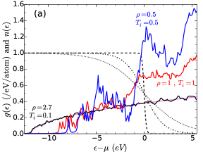
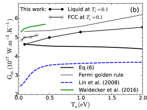
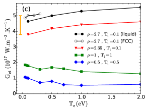
Figure 1: (color online) (a) DOS of Al with $T_{i}=T_{e}$ and Fermi-Dirac distribution (dashed lines) for three electronic temperatures at $T_{e}=0.1,1,2$ eV. The violet line is the DOS of the free-electron gas at $2.7$ $\rm g.cm^{-3}$. Energy is measured with respect to the chemical potential $\mu(\rho,T_{e})$. (b) $G_{ei}(T_{e},T_{i})$ vs $T_{e}$ for solid density Al at $T_{i}=0.1$ eV compared with other model predictions (see all table 1). (c) $G_{ei}(T_{e},T_{i})$ vs $T_{e}$ for Al at various densities and ionic temperatures. The vertical bar indicates the magnitude of the variation of $G_{ei}$ at melting.

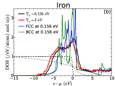
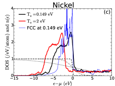
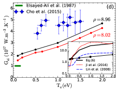
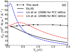
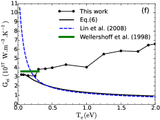
Figure 2: (color online) Top panels: same as Fig. 1a for Cu, Fe and Ni at the conditions indicated in the legends. Bottom panels: $G(T_{e},T_{i})$ vs $T_{e}$ for (d) solid and liquid density Cu at $T_{i}=0.2$ eV, (e) solid density Fe at $T_{i}=0.156$ eV, and (f) solid density Ni at $T_{i}=0.149$ eV. In each case, the full lines with circles show the work’s results, the full lines without symbols are obtained using Eq.(6) with $G_{0}^{ei}$ set to reproduce the lowest $T_{e}$ value, the long dashed lines are the results based on Eq.(5) discussed in Lin_et_al_2008 . In panel (d), the diamonds show the experimental results of Cho_et_al_2015 , the bold green segment shows the measurement of Elsayed_et_al_1987 for solid Cu. In the inset, the dashed lines show the model predictions based on Eq.(5) presented in Lin_et_al_2008 ; JiZhang2016 . In panel (f), the bold green segment shows the measurement of Wellershoff1998 .

By following techniques similar to those used for the ab-initio calculation of electronic conductivitiesHolst2011 , we use the ionic and electronic structures calculated with standard quantum molecular dynamics simulations to evaluate the Kubo relations (3) needed in Eq.(2). Briefly, for each ionic configuration ${\bf R}$, the electronic structure is obtained from the solution of the Kohn-Sham equations $\big{(}\frac{\hat{{\bf p}}^{2}}{2m_{e}}+V_{KS}[\rho_{e},{\bf R}]\big{)}|\alpha\rangle=\epsilon_{\alpha}|\alpha\rangle$, where $\epsilon_{\alpha}$ and $|\alpha\rangle$ are the single-particle Kohn-Sham energies and states, $\rho_{e}({\bf r})=\sum_{\alpha}{n_{\alpha}|\langle{\bf r}|\alpha\rangle|^{2}}$ is the electron density, and $n_{\alpha}=n(\epsilon_{\alpha})$ with $n(\epsilon)=\left(1+e^{-(\mu-\epsilon)/k_{B}T_{e}}\right)^{-1}$ represents the Fermi-Dirac occupation number of the state $\alpha$. In terms of the Kohn-Sham quantities, it can be shown that the coupling coefficients (3)

$$\gamma_{Ix,Jy} = -\frac{\pi}{m_{i}}{\sum_{\alpha,\beta}}^{\prime}{\frac{n_{\alpha}-n_{\beta}}{\epsilon_{\alpha\beta}}f_{Ix}^{\alpha\beta}f_{Jy}^{\beta\alpha}\delta\left(\epsilon_{\alpha\beta}/\hbar\right)}\,,$$ (4)

where the matrix elements $f_{Ix}^{\alpha\beta}=\left\langle\alpha\big{|}\hat{f}_{Ix}^{(sc)}\big{|}\beta\right\rangle$ and $\hat{f}_{Ix}^{(sc)}$ is the effective force along the $x$-direction between ion $I$ and a Kohn-Sham electron screened by the other electrons.

Before showing results, we relate our approach to a model that has served as a reference in recent works,

$$G_{\rm e-ph}\approx G_{0}^{\rm e-ph}\!\!\int\limits_{-\infty}^{\infty}{\left[\frac{g(\epsilon)}{g(\epsilon_{F})}\right]^{2}\!\!\left(\!-\frac{\partial\,n(\epsilon)}{\partial\epsilon}\right)\!d\epsilon}\,,$$ (5)

which is a simplification in the high temperature limit Wang1994 ; Lin_et_al_2008 of the general electron-phonon coupling fomula Allen1987 . Here $g(\epsilon)$ is the electron density of states (DOS), which is computable with DFT, and $G_{0}^{\rm e-ph}=\pi\hbar k_{B}\lambda\langle\omega^{2}\rangle g(\epsilon_{F})$, where $\epsilon_{F}=k_{B}T_{F}$ is the Fermi energy, $\langle\omega^{2}\rangle$ is the second moment of the phonon spectrum, and $\lambda$ is the electron-phonon mass enhancement factor. In previous works, the prefactor $G_{0}^{\rm e-ph}$ was either set to match an experimental measurement at low electronic temperature Lin_et_al_2008 , or was calculated ab-initio Waldecker2016 ; JiZhang2016 . Although derived for crystalline solids, the model (5) was used in recent works on warm dense matter systems Leguay2013 ; Cho_et_al_2015 ; Dorchies2016 ; Jourdain_et_al_2018 ; Ogitsu2018 . Remarkably, an expression similar to Eq.(5) also results from Eq.(4) if one assumes that the matrix elements $f_{Ix}^{\alpha\beta}$ depend weakly on the energies, $f_{Ix}^{\alpha\beta}\approx f_{Ix}$, which yields

$$G_{ei}\approx G_{0}^{ei}\int\limits_{-\infty}^{\infty}{\left[\frac{g(\epsilon)}{g(\epsilon_{F})}\right]^{2}\!\!\left(\!-\frac{\partial\,n(\epsilon)}{\partial\epsilon}\right)d\epsilon}\,,$$ (6)

where $G_{0}^{ei}=|f_{Ix}|^{2}g(\epsilon_{F})^{2}$. The formulas (5) and (6) highlights the interplay between the DOS and the distribution of electronic states, which, as shown by Lin et al. Lin_et_al_2008 , results in a strong dependence on the chemical composition and often on sharp variations with $T_{e}$. Below we compare our results to predictions based on (5) reported by others and on Eq.(6) with $G_{0}^{ei}$ set to reproduce the value of $G_{ei}$ at the lowest $T_{e}$ considered. We find that the simplified models (5) and (6) tend to overestimate the dependence on $T_{e}$ or predicts variations at odds with the full calculation.

Figures 1 and 2 (bottom panels) show results for $G_{ei}(T_{e},T_{i})$ for five representative materials and physical conditions, together with the predictions of previous models and with experimental data. Below we highlight some of the key findings. For each element, the upper panels show the electron density of states $g(\epsilon)$ and the Fermi-Dirac distribution function $n(\epsilon)$ at representative conditions. Our results were obtained with the open-source Quantum Espresso program QuantumEspressoCode ; the simulation details are given in the Supplemental Material SM . In all cases, the material is prepared in the disordered, liquid-like state, except for Aluminum for which we also show calculations in a finite-temperature FCC configuration. In the figures, temperatures $T_{i,e}$ are in eV and the material densities $\rho$ are in $\rm g.cm^{-3}$.

Aluminum. Figure 1b shows $G_{ei}(T_{i},T_{e})$ versus $T_{e}$ at solid density $\rho\!=\!2.7$ $\rm g.cm^{-3}$ and $T_{i}=0.1$ eV (slightly above the melting temperature $0.08$ eV), together with other model predictions, including the Fermi golden rule evaluated using the same pseudopotential $v_{ie}$ of the ab-initio calculations, and predicitons based on Eq.(6) and the results of Lin_et_al_2008 and Waldecker2016 based on Eq.(5) (see table 1 for other predictions). $G_{ei}$ steadily increases between $4.6$ to $5.6$ $10^{17}\,\rm W/Km^{3}$ in the range $0.1\leq T_{e}\leq 2$ eV, as a result of the growing number of excited electrons that participate to the electron-ion scattering processes. Our results are in best agreement with the Fermi-golden rule, which is expected given the free electron-like character of Al at solid density (see full black and violet lines in Fig. 1). They differ from the prediction based on Eq.(6), which is similar to the result one obtains with the DOS of the free-electron gas at solid density (see Fig. 1d in Lin_et_al_2008 ). Figure 1c shows $G_{ei}$ at other mass densities $\rho$ and ionic temperatures $T_{i}$. As $\rho$ decreases, the DOS shown in Fig. 1a progressively loses its free electron-like character. We find that the $G_{ei}$ decreases with $\rho$ at constant $T_{e}$, which is essentially an effect of the variation of the decreasing electron density (see $n_{e}$ prefactor in Eq.(2)), and its variation with $T_{e}$ changes from an overall increasing to a decreasing functions of $T_{e}$. The figures also show calculations obtained for FCC lattices at solid density (open circles in Fig 1b and c). Our results are in good agreement with the result of Waldecker et al. Waldecker2016 based on Eq.(5) with a DFT calculation of $G_{0}^{\rm e-ph}$. At melting, the density is known to decrease from $\sim 2.7$ to $\sim 2.35$ $\rm g.cm^{-3}$ Leitner2017 and $G_{ie}$ decreases by about $25\%$, as indicated by the orange vertical bar in Fig. 1c. This should be contrasted with the large change in the electrical resisitivity at melting, which increases by a factor $\sim 2.1$ Leitner2017 , in other words disorder has a higher effect on momentum relaxation than on energy relaxation.

Copper. Warm dense copper has been the focus of several recent studies Cho_et_al_2015 ; Jourdain_et_al_2018 ; Lin_et_al_2008 ; JiZhang2016 . Figure 2d shows results at solid and melt densities, $8.96$ and $8.02$ $\rm g.cm^{-3}$, and $T_{i}=0.2$ eV (melting temperature is $0.117$ eV), together with the measurements of Elsayed_et_al_1987 and Cho_et_al_2015 ; the inset compares our result at $8.96$ $\rm g.cm^{-3}$ with Eq.(6) and with the results of Lin_et_al_2008 and JiZhang2016 based on Eq(5). We find that $G_{ei}$ increases with $T_{e}$, with a faster variation above $0.5$ eV when the $d$ electrons, which are responsible for the prominent regions of high DOS in Fig. 2a, can be excited and participate the electron-ion energy exchanges. However, the variation is not as sharp and intense as that predicted using Eq.(5) of Lin_et_al_2008 and JiZhang2016 . Unlike Ref. Lin_et_al_2008 , we don’t find a sharp increase of $G_{ei}$ at small $T_{e}$, which was ascribed to the thermal excitations of d-electrons. At solid density, we find $G_{ei}\simeq 2$ $10^{17}\,\rm W/Km^{3}$, in fair agreement with the old measurement $10^{17}\,\rm W/Km^{3}$ of Elsayed-Ali et al. Elsayed_et_al_1987 for solid Cu. Our data lie slightly below the recent measurements reported in Cho_et_al_2015 .

Iron. Figure 2e shows the variation of $G_{ei}$ with $T_{e}\leq 2$ eV for solid density Fe $\rho=7.87$ $\rm g.cm^{-3}$ at melting temperature $T_{i}=0.156$ eV. We find that $G_{ei}$ does not vary significantly over the temperature range considered, unlike the predictions based on Eqs.(5) Lin_et_al_2008 and (6).

Nickel. Figure 2f shows the variation of $G_{ei}$ with $T_{e}\leq 2$ eV for solid density Ni $\rho=8.91$ $\rm g.cm^{-3}$ at melting temperature $T_{i}=0.149$ eV. We find that $G_{ei}$ increases from $3.1$ to $5.6$ $10^{17}\,\rm W/Km^{3}$ over the temperature range, in contrast with the results based on Eq.(5) Lin_et_al_2008 and on Eq.(6). Our result at lower $T_{e}$ are in good agreement with the measurement reported by Wellershoff et al. Wellershoff1998 .

In summary, we have presented much-needed first-principles calculations of the electron-ion coupling factors of materials at the confluence of solids and plasmas based on a general expression in terms of the friction coefficients felt by ions due to the non-adiabatic electron-ion interactions. The approach serves as a useful comparison with the experimental measurements, permits an extension into conditions not covered by experiments, and provides insight into the underlying physics. We hope that this work will help assist and motivate future experiments and, ultimately, will help advance our understanding of the warm dense matter regime.

- (1) Frontiers and Challenges in Warm Dense Matter, Lecture Notes in Computational Science and Engineering, Vol. 96, edited by F. Graziani, M.P. Desjarlais, R. Redmer and S.B. Trickey (Springer, New York, 2014).
- (2) Plasma: at the frontier of scientific discovery, US Department of Energy Report of the Panel on Frontiers of Plasma Science, 2017, Chapter 1, available at https://science.energy.gov/fes/community-resources/workshop-reports/ .
- (3) A. Ng, P. Celliers, G. Xu and A. Forsman, Phys. Rev. E 52, 4299 (1995).
- (4) Fäustlin, R. R. and Bornath, Th. and Döppner, T. and Düsterer, S. and Förster, E. and Fortmann, C. and Glenzer, S. H. and Göde, S. and Gregori, G. and Irsig, R. and Laarmann, T. and Lee, H. J. and Li, B. and Meiwes-Broer, K.-H. and Mithen, J. and Nagler, B. and Przystawik, A. and Redlin, H. and Redmer, R. and Reinholz, H. and Röpke, G. and Tavella, F. and Thiele, R. and Tiggesbäumker, J. and Toleikis, S. and Uschmann, I. and Vinko, S. M. and Whitcher, T. and Zastrau, U. and Ziaja, B. and Tschentscher, Th., Phys. Rev. Lett. 104, 125002 (2010).
- (5) A. Ng, Int. J. Quant. Chem. 112, 150 (2012).
- (6) P. M. Leguay, A. Lévy, B. Chimier, F. Deneuville, D. Descamps, C. Fourment, C. Goyon, S. Hulin, S. Petit, O. Peyrusse, J. J. Santos, P. Combis, B. Holst, V. Recoules, P. Renaudin, L. Videau, and F. Dorchies, Phys. Rev. Lett. 111, 245004 (2013).
- (7) B. I. Cho, T. Ogitsu, K. Engelhorn, A. A. Correa, Y. Ping, J. W. Lee, L. J. Bae, D. Prendergast, R. W. Falcone, and P. A. Heimann, Scientific Reports 6, 18843 (2016).
- (8) F. Dorchies and V. Recoules, Phys. Rep. 657, 1 (2016).
- (9) N. Jourdain, L. Lecherbourg, V. Recoules, P. Renaudin, and F. Dorchies, Phys. Rev. B 97, 075148 (2018).
- (10) T. Ogitsu, A. Fernandez-Pañella, S. Hamel, A. A. Correa, D. Prendergast, C. D. Pemmaraju, and Y. Ping, Phys. Rev. B 97, 214203 (2018).
- (11) J. Daligault and G. Dimonte, Phys. Rev. E 79, 056403 (2009).
- (12) Z. Chen, B. Holst, S. E. Kirkwood, V. Sametoglu, M. Reid, Y. Y. Tsui, V. Recoules, and A. Ng, Phys. Rev. Lett. 110, 135001 (2013).
- (13) J. Clérouin, G. Robert, P. Arnault, C. Ticknor, J.D. Kress, and L.A. Collins, Phys. Rev. E 91, 011101(R) (2015).
- (14) A.B. Zylstra, J. A. Frenje, P. E. Grabowski, C. K. Li, G. W. Collins, P. Fitzsimmons, S. Glenzer, F. Graziani, S. B. Hansen, S. X. Hu, M.G. Johnson, P. Keiter, H. Reynolds, J. R. Rygg, F. H. Séguin, and R. D. Petrasso, Phys. Rev. Lett. 114, 215002 (2015).
- (15) H. Brysk et al., Plasma Phys. 17, 473 (1975).
- (16) G. Hazak, Z. Zinamon, Y. Rosenfeld, and M. W. C. Dharma-wardana, Phys. Rev. E 64, 066411 (2001).
- (17) J. Daligault and D. Mozyrsky, High Energy Density Phys. 4, 58 (2008).
- (18) M.W.C. Dharma-wardana, Phys. Rev. E 64, 035401(R) (2001).
- (19) J. Vorberger and D.O. Gericke, AIP Conf. Proc. 1464, 572 (2012)
- (20) Z. Lin, L. V. Zhigilei, and V. Celli, Phys. Rev. B 77, 075133 (2008); data available at the address http://www.faculty.virginia.edu/CompMat/electron-phonon-coupling/
- (21) L. Waldecker, R. Bertoni, R. Ernstorfer, and J. Vorberger, Phys. Rev. X 6, 021003 (2016). See DFT line in Figure (3c).
- (22) M.P. Desjarlais, J.D. Kress and L.A. Collins, Phys. Rev. E 66, 025401(R) (2002).
- (23) B. Holst, M. French, and R. Redmer, Phys. Rev. B 83, 235120 (2011).
- (24) T. Sjostrom and J. Daligault, Phys. Rev. E 92, 063304 (2015).
- (25) J. Simoni and J. Daligault, in preparation.
- (26) J. Daligault and D. Mozyrsky, Phys. Rev. E 75, 026402 (2007).
- (27) J. Daligault and D. Mozyrsky, Phys. Rev. B 98, 205120 (2018).
- (28) N.W. Ashcroft and N.D. Mermin, Solid State Physics (Harcourt College Publishers, 1976); table 23.3.
- (29) P.B. Allen, Phys. Rev. Lett. 59, 1460 (1987).
- (30) X.Y. Wang, D.M. Riffe, Y.-S. Lee, and M.C. Downer, Phys. Rev. B 50, 8016 (1994).
- (31) P. Giannozzi, O. Andreussi, T. Brumme, O. Bunau, M. Buongiorno Nardelli, M. Calandra, R. Car, C. Cavazzoni, D. Ceresoli, M. Cococcioni, N. Colonna, I. Carnimeo, A. Dal Corso, S. de Gironcoli, P. Delugas, R. A. DiStasio Jr, A. Ferretti, A. Floris, G. Fratesi, G. Fugallo, R. Gebauer, U. Gerstmann, F. Giustino, T. Gorni, J Jia, M. Kawamura, H.-Y. Ko, A. Kokalj, E. Küçükbenli, M .Lazzeri, M. Marsili, N. Marzari, F. Mauri, N. L. Nguyen, H.-V. Nguyen, A. Otero-de-la-Roza, L. Paulatto, S. Poncé, D. Rocca, R. Sabatini, B. Santra, M. Schlipf, A. P. Seitsonen, A. Smogunov, I. Timrov, T. Thonhauser, P. Umari, N. Vast, X. Wu, S. Baroni, J. Phys.: Condens. Matter 29, 465901 (2017).
- (32) See Supplemental Material at xxxx for the details of the quantum molecular dynamics simulations.
- (33) M. Leitner, T. Leitner, A. Schmon, K. Aziz, and G. Pottlacher, Metallurgical and Materials Transactions A 48A, 3036 (2017); Figures 1 and 2.
- (34) P. Ji and Y. Zhang, Phys. Lett. A 380, 1551 (2016). See Figure (2e).
- (35) H. E. Elsayed-Ali, T. B. Norris, M. A. Pessot, and G. A. Mourou, Phys. Rev. Lett. 58, 1212 (1987).
- (36) S.-S. Wellershoff, J. Güdde, J. Hohlfeld, J. G. Müller and E. Matthias, Proc. SPIE 3343, 378 (1998).