Quantum-classical correspondence of work distributions for initial states with quantum coherence

Abstract

The standard definition of quantum fluctuating work is based on the two-projective energy measurement, which however does not apply to systems with initial quantum coherence because the first projective energy measurement destroys the initial coherence, and affects the subsequent evolution of the system. To address this issue, several alternative definitions, such as those based on the full counting statistics and the Margenau-Hill distribution, have been proposed recently. These definitions seem ad hoc because justifications for them are still lacking. In the current study, by utilizing the quantum Feynman-Kac formula and the phase space formulation of quantum mechanics, we prove that the leading order of work distributions is equal to the classical work distribution. Thus we prove the validity of the quantum-classical correspondence of work distributions for initial states with quantum coherence, and provide some justification for those definitions of work. We use an exactly solvable model of the linearly dragged harmonic oscillator to demonstrate our main results.

I Introduction

Traditionally, thermodynamics describes the energy conversions of macroscopic systems, in which thermodynamic variables, such as work, heat, and entropy production are quantities of ensemble average. Fluctuations of these quantities are vanishingly small and are usually ignored. However, at the microscopic scale, fluctuations are too prominent to be ignored. In the past two decades, stochastic thermodynamics emerges as a new field Jarzynski (2011); Seifert (2012); Sekimoto (1998, 2010); Li et al. (2010); Martínez et al. (2016); Bang et al. (2018), in which the classical fluctuating work is defined along individual trajectories in the phase space Jarzynski (1997); Sekimoto (1998, 2010), leading to the striking results of the fluctuation theorems Jarzynski (1997); Crooks (1999); Seifert (2005); Hummer and Szabo (2001); Kawai et al. (2007); Esposito and van den Broeck (2010); Gong and Quan (2015); Liphardt et al. (2002); Collin et al. (2005); Douarche et al. (2006); Junier et al. (2009); Toyabe et al. (2010); Pekola (2015); Hoang et al. (2018). Nevertheless, in the quantum regime, there is some ambiguity in the definition of the stochastic trajectory and the corresponding quantum work functional Talkner and Hänggi (2016); Funo and Quan (2018a, b) due to the existence of the uncertainty principle.

In quantum thermodynamics Kurchan (2000); Tasaki (2000); Talkner et al. (2007); Talkner and Hänggi (2016); Funo and Quan (2018a, b); Brandner and Seifert (2016); Suomela et al. (2016); Liu (2016); Wang (2018); Liu and Xi (2016); Rogers (2017); Aurell (2018); Sampaio et al. (2016); Jaramillo et al. (2017); Gong et al. (2016); Talarico et al. (2016); Bartolotta and Deffner (2018); Silveri et al. (2017); Frenzel et al. (2016); Guarnieri et al. (2018); Kwon and Kim (2018); Peng and Fan (2017); Strasberg (2018); Goold et al. (2016), a standard definition of quantum fluctuating work is given by the energy difference between the initial and the final outcomes of the two-projective energy measurement (TPM) Kurchan (2000); Tasaki (2000); Talkner et al. (2007). Based on this definition, the fluctuation theorems, such as the Jarzynski equality and the Crooks relation can be obtained straightforwardly Jarzynski (2011); Seifert (2012); Kurchan (2000); Tasaki (2000); Talkner et al. (2007). The TPM approach provides an operational way to measure the work in both isolated and open quantum systems, and the fluctuation theorems in the quantum regime have been tested experimentally using the TPM Huber et al. (2008); Batalhão et al. (2014); An et al. (2015). In addition, it has been shown Jarzynski et al. (2015); Zhu et al. (2016); Wang and Quan (2017); Fei et al. (2018); García-Mata et al. (2017); Arrais et al. (2018); García-Mata et al. (2018) that the definition of quantum fluctuating work based on the TPM obeys the quantum-classical correspondence principle, which provides some justification for this definition of quantum fluctuating work.

In spite of its success in the study of quantum thermodynamics, the TPM approach has its limitations which have been pointed out in recent studies Perarnau-Llobet et al. (2017); Lostaglio (2018); Bäumer et al. (2018). For states with quantum coherence, the first projective energy measurement destroys the coherence, and affects the subsequent evolution of the system Allahverdyan (2014); Solinas and Gasparinetti (2015); Hofer and Clerk (2016); Solinas and Gasparinetti (2016); Solinas et al. (2017); Miller and Anders (2017, 2018); Bäumer et al. (2018); Perarnau-Llobet et al. (2017); Lostaglio (2018); Åberg (2018); Sampaio et al. (2018); Talkner and Hänggi (2016); Francica et al. (2017); Xu et al. (2018, 2019); Wu et al. (2019). Thus the averaged work is no longer equal to the difference of the internal energy (expectation value of the Hamiltonian) before and after the evolution. As a result, alternative definitions of quantum fluctuating work have been proposed for initial states with quantum coherence Allahverdyan and Nieuwenhuizen (2005); Allahverdyan (2014); Margenau and Hill (1961); Solinas and Gasparinetti (2015); Hofer and Clerk (2016); Solinas and Gasparinetti (2016); Solinas et al. (2017); Nazarov and Kindermann (2003); Miller and Anders (2017); Sampaio et al. (2018); Talkner and Hänggi (2016). Examples include that based on the full counting statistics (FCS) Solinas and Gasparinetti (2015); Hofer and Clerk (2016); Solinas and Gasparinetti (2016); Solinas et al. (2017); Nazarov and Kindermann (2003), and that based on the Margenau-Hill distribution (MH) Allahverdyan (2014); Margenau and Hill (1961). The two definitions are related to the weak measurement that circumvents the invasive effect of the measurement disturbance on the statistics of work, and they are experimentally operational Solinas and Gasparinetti (2015); Hofer and Clerk (2016); Solinas and Gasparinetti (2016); Solinas et al. (2017); Nazarov and Kindermann (2003); Allahverdyan (2014); Margenau and Hill (1961); Johansen (2007); Lundeen and Bamber (2012). When the initial state has no quantum coherence, the two definitions are equivalent to that based on the TPM Bäumer et al. (2018); Perarnau-Llobet et al. (2017); Talkner and Hänggi (2016). When the initial state has quantum coherence, the probabilities of work distributions are not positive-definite. In other words, they are quasi-probabilities Bäumer et al. (2018); Perarnau-Llobet et al. (2017); Hofer and Clerk (2016); Miller and Anders (2017). For this reason, a no-go theorem for definitions of quantum work is proposed Perarnau-Llobet et al. (2017); Lostaglio (2018); Bäumer et al. (2018); Wu et al. (2019).

In the current study, we investigate the definitions of quantum fluctuating work based on the FCS and the MH from the perspective of quantum-classical correspondence. Inspired by Refs. Jarzynski et al. (2015); Fei et al. (2018) which studied the quantum-classical correspondence of quantum work distribution based on the TPM, we apply the same method of the phase space formulation of quantum mechanics Wigner (1932); Hillery et al. (1984); Polkovnikov (2010); Fei et al. (2018), and find that even in the presence of quantum coherence, both quantum work distributions converge to their classical counterpart in the limit of $\hbar\rightarrow 0$, where $\hbar$ is Planck’s constant. In addition, we show that in comparison with the classical work, the two definitions of quantum fluctuating work lead to different quantum corrections Wigner (1932); Fei et al. (2018). Our results thus provide some justification for the validity of the definitions of quantum fluctuating work based on the FCS and the MH.

This paper is organized as follows. In Sec. II, we investigate the work characteristic functions based on the FCS and the MH by utilizing the quantum Feynman-Kac formula Kac (1949); Liu (2012); Fei et al. (2018) and the phase space formulation of quantum mechanics Wigner (1932); Hillery et al. (1984); Polkovnikov (2010); Fei et al. (2018), and give our main results. In Sec. III, we use an exactly solvable model of the linearly dragged harmonic oscillator to demonstrate our main results. In Sec. IV, we give some discussions and conclude our paper.

II Quantum-classical correspondence of the Feynman-Kac formula

Our setup is an isolated quantum system with an initial state described by a density matrix $\hat{\rho}(0)$. The system is driven by an external agent from the initial time $t=0$ to the final time $t=\tau$. Accordingly, the Hamiltonian of the system is time-dependent $\hat{H}(t)$ that evolves from the initial time $t=0$ to the final time $t=\tau$. The unitary evolution operator is

$$\hat{U}(\tau)=\overleftarrow{\mathcal{T}}\exp\left[-\frac{\mathrm{i}}{\hbar}\int_{0}^{\tau}\mathrm{d}t\hat{H}(t)\right],$$ (1)

where $\overleftarrow{\mathcal{T}}$ is the time-ordered operator. During the whole driving process, external work $W$ is exerted on the system. In this paper, we study the characteristic function of the work distribution $P(W)$:

$$\Phi(\eta):=\int_{-\infty}^{+\infty}\mathrm{d}WP(W)\mathrm{e}^{\mathrm{i}\eta W}.$$ (2)

If the initial state $\hat{\rho}(0)$ does not have quantum coherence, i.e., it is diagonal in the energy eigenbasis of $\hat{H}(0)$, we can adopt the TPM approach to define the quantum fluctuating work, and the characteristic function of work can be expressed as Talkner et al. (2007):

$$\Phi_{\text{TPM}}(\eta)=\text{Tr}\left[\mathrm{e}^{\mathrm{i}\eta\hat{H}(\tau)}\hat{U}(\tau)\mathrm{e}^{-\mathrm{i}\eta\hat{H}(0)}\hat{\rho}(0)\hat{U}^{\dagger}(\tau)\right].$$ (3)

If $\hat{\rho}(0)$ has quantum coherence, it does not commute with the initial Hamiltonian $\hat{H}(0)$, i.e., $\left[\hat{\rho}(0),\hat{H}(0)\right]\neq 0$. In Ref. Solinas and Gasparinetti (2015), Solinas and Gasparinetti studied the quantum fluctuating work using the FCS. They gave the following definition of the characteristic function of work Solinas and Gasparinetti (2015):

$$\Phi_{\text{FCS}}(\eta)=\text{Tr}\left[\mathrm{e}^{\mathrm{i}\eta\hat{H}(\tau)}\hat{U}(\tau)\mathrm{e}^{-\mathrm{i}\frac{\eta}{2}\hat{H}(0)}\hat{\rho}(0)\mathrm{e}^{-\mathrm{i}\frac{\eta}{2}\hat{H}(0)}\hat{U}^{\dagger}(\tau)\right].$$ (4)

The FCS is not the only way to characterize non-invasive measurements of work. In Ref. Allahverdyan (2014), Allahverdyan proposed another definition of the quantum fluctuating work based on the MH distribution for successive energy measurements Allahverdyan (2014); Margenau and Hill (1961); Johansen (2007); Lundeen and Bamber (2012):

$$\Phi_{\text{MH}}(\eta)=\text{Tr}\left[\mathrm{e}^{\mathrm{i}\eta\hat{H}(\tau)}\hat{U}(\tau)\left(\mathrm{e}^{-\mathrm{i}\eta\hat{H}(0)}\star\hat{\rho}(0)\right)\hat{U}^{\dagger}(\tau)\right],$$ (5)

where $\hat{A}\star\hat{B}:=\frac{1}{2}\left[\hat{A}\hat{B}+\hat{B}\hat{A}\right]$.

Comparing Eqs. (4) and (5) with Eq. (3), we can see that $\Phi_{\text{FCS}}(\eta)$ and $\Phi_{\text{MH}}(\eta)$ are two types of symmetrization of $\Phi_{\text{TPM}}(\eta)$. They are introduced to deal with the situation when the initial state has quantum coherence (the initial state $\hat{\rho}(0)$ does not commute with the initial Hamiltonian $\hat{H}(0)$). While the first and the second moments of work, $\langle W\rangle$ and $\langle W^{2}\rangle$, are the same for $\Phi_{\text{FCS}}(\eta)$ and $\Phi_{\text{MH}}(\eta)$, higher-order moments in general are different Miller and Anders (2018). It is worth mentioning that when the initial state has no coherence, the three definitions of quantum fluctuating work are equivalent.

II.1 Phase space formulation of quantum Feynman-Kac formula

In this section, we investigate the time evolution of the operators included in the trace of Eqs. (4) and (5). For $\Phi_{\text{FCS}}(\eta)$ [Eq. (4)], let us define an operator $\hat{K}(t)$ as

$$\hat{K}(t):=\mathrm{e}^{\mathrm{i}\eta\hat{H}(t)}\hat{U}(t)\mathrm{e}^{-\mathrm{i}\frac{\eta}{2}\hat{H}(0)}\hat{\rho}(0)\mathrm{e}^{-\mathrm{i}\frac{\eta}{2}\hat{H}(0)}\hat{U}^{\dagger}(t).$$ (6)

It is easy to prove that $\hat{K}(t)$ satisfies the quantum Feynman-Kac formula introduced in Refs. Liu (2012); Fei et al. (2018):

$$\partial_{t}\hat{K}(t)=-\frac{\mathrm{i}}{\hbar}\left[\hat{H}(t),\hat{K}(t)\right]+\left[\partial_{t}\mathrm{e}^{\mathrm{i}\eta\hat{H}(t)}\right]\mathrm{e}^{-\mathrm{i}\eta\hat{H}(t)}\hat{K}(t).$$ (7)

The initial condition is

$$\hat{K}(0)=\mathrm{e}^{\mathrm{i}\frac{\eta}{2}\hat{H}(0)}\hat{\rho}(0)\mathrm{e}^{-\mathrm{i}\frac{\eta}{2}\hat{H}(0)}.$$ (8)

We reformulate Eq. (7) in the phase space (Weyl-Wigner) representation of quantum mechanics Wigner (1932); Hillery et al. (1984); Polkovnikov (2010); Fei et al. (2018) as follows

$$\partial_{t}K(z,t) = \frac{2}{\hbar}H(z,t)\sin\left(\frac{\hbar}{2}\Lambda\right)K(z,t)$$ (9)

$$+\Omega(z,t)\exp\left(\frac{\mathrm{i}\hbar}{2}\Lambda\right)K(z,t).$$

This equation describes the time evolution of the function $K(z,t)$, which is the Weyl symbol of the operator $\hat{K}(t)$. Here $z=(x,p)$ represents a point in the phase space, and $x$ is the position and $p$ is the momentum of the particle. In Eq. (9), $H(z,t)$ is the Weyl symbol of the Hamiltonian $\hat{H}(t)$. In this paper, for simplicity, we study a system described by the following Hamiltonian

$$\hat{H}(t)=\frac{\hat{p}^{2}}{2m}+V(\hat{x},t),$$ (10)

where $m$ is the mass of the single particle, and $V$ is the potential. The symplectic operator $\Lambda$ Hillery et al. (1984) is

$$\Lambda=\overleftarrow{\partial_{x}}\overrightarrow{\partial_{p}}-\overleftarrow{\partial_{p}}\overrightarrow{\partial_{x}},$$ (11)

and the arrows denote the directions the partial derivatives act upon. In Eq. (9),

$$\Omega(z,t)=\left\{\partial_{t}\mathrm{e}^{\mathrm{i}\eta\hat{H}(t)}\right\}_{w}\exp\left(\frac{\mathrm{i}\hbar}{2}\Lambda\right)\left\{\mathrm{e}^{-\mathrm{i}\eta\hat{H}(t)}\right\}_{w},$$ (12)

where $\{\cdot\}_{w}$ denotes the Weyl symbol of the operator included in the bracket, and $\exp\left(\frac{\mathrm{i}\hbar}{2}\Lambda\right)$ denotes the star product Hillery et al. (1984). Then according to Eq. (4), the characteristic function of quantum work can be calculated as

$$\Phi(\eta)=\int_{-\infty}^{+\infty}\mathrm{d}zK(z,\tau),$$ (13)

where the integral over $\mathrm{d}z$ denotes the integral over the whole phase space.

Having introduced the phase space formulation of quantum Feynman-Kac formula, in the following, we study the quantum work statistics and its relation to the classical work statistics.

II.2 Quantum work statistics and its classical counterpart

As pointed out by Wigner in 1932 Wigner (1932), the phase space representation has advantages in studying the quantum-classical correspondence and calculating the quantum corrections on thermodynamic variables in powers of $\hbar$. In this subsection, we calculate the work statistics by solving Eq. (9). Let us recall that when studying the Weyl symbol of the exponential of the Hamiltonian $\mathrm{e}^{-\mathrm{i}\eta\hat{H}(t)}$, for example, the density matrix of the thermal equilibrium state $\hat{\rho}^{eq}(0)\propto\mathrm{e}^{-\beta\hat{H}(0)}$ ($\beta$ is the inverse temperature), Wigner found that it can be expanded as Wigner (1932)

$$\left\{\mathrm{e}^{-\mathrm{i}\eta\hat{H}(t)}\right\}_{w}=\mathrm{e}^{-\mathrm{i}\eta H(z,t)}\left[1+(\mathrm{i}\hbar)^{2}f(\mathrm{i}\eta,z,t)+\mathcal{O}(\hbar^{4})\right],$$ (14)

where

$$f(\mathrm{i}\eta,z,t)=\frac{(\mathrm{i}\eta)^{2}}{8m}\left[\partial_{x}^{2}V-\frac{\mathrm{i}\eta}{3}\left(\partial_{x}V\right)^{2}-\frac{\mathrm{i}\eta}{3m}p^{2}\partial_{x}^{2}V\right].$$ (15)

Please note that on the r.h.s. of Eq. (14), there are no terms proportional to odd orders of $\hbar$, and this feature is important for our later analysis. By substituting Eqs. (12) and (14) into Eq. (9) and expanding Eq. (9) in powers of $\hbar$, we obtain

$$\partial_{t}K= H\Lambda K+\mathrm{i}\eta\partial_{t}HK$$ (16)

$$+\frac{\mathrm{i}\hbar}{2}\left[(\mathrm{i}\eta)^{2}(H\Lambda\partial_{t}H)+\mathrm{i}\eta\partial_{t}H\Lambda\right]K+\mathcal{O}(\hbar^{2}).$$

By expanding $K(z,t)$ in powers of $\hbar$:

$$K(z,t)=K^{(0)}(z,t)+(\mathrm{i}\hbar)K^{(1)}(z,t)+(\mathrm{i}\hbar)^{2}K^{(2)}(z,t)+\cdots,$$ (17)

and identifying terms of the same orders of $\hbar$ in Eq. (16), we obtain

$$\partial_{t}K^{(0)}= H\Lambda K^{(0)}+\mathrm{i}\eta\partial_{t}HK^{(0)};$$

$$\partial_{t}K^{(1)}= H\Lambda K^{(1)}+\mathrm{i}\eta\partial_{t}HK^{(1)}$$

$$+\frac{1}{2}\left[(\mathrm{i}\eta)^{2}(H\Lambda\partial_{t}H)+\mathrm{i}\eta\partial_{t}H\Lambda\right]K^{(0)};$$

$$\cdots$$ (18)

The initial conditions [Eq. (8)] in the phase space representation are (see Appendix A)

$$K^{(0)}(z,0) = P^{(0)}(z,0);$$

$$K^{(1)}(z,0) = \frac{\mathrm{i}\eta}{2}H(z,0)\Lambda P^{(0)}(z,0);$$ (19)

$$\cdots$$

where $P^{(0)}(z,0)$ denotes the zeroth-order term of the Weyl symbol of the initial density matrix $\hat{\rho}(0)$, and it will be defined later [see Eq. (21)]. We regard $P^{(0)}(z,0)$ as the classical counterpart of $\hat{\rho}(0)$:

$$P_{\text{Classical}}(z,0):=P^{(0)}(z,0).$$ (20)

It can be checked Wigner (1932) that for the quantum thermal equilibrium state, $P^{(0)}(z,0)$ is exactly the thermal equilibrium state of the classical Hamiltonian $H(z,0)$.

Please note that not all quantum states have the classical counterparts in general. For example, the Fock states in quantum optics or the spin states in spin systems do not have well-defined classical counterparts. However, for systems described by Eq. (10), the thermal equilibrium state Wigner (1932) and those evolved from the thermal equilibrium state have well-defined classical counterparts in the phase space. For simplicity, we focus on those states evolved from the thermal equilibrium state in the following discussions. The Wigner functions of these states have the following form in powers of $\hbar$:

$$P(z,0)=P^{(0)}(z,0)+(\mathrm{i}\hbar)^{2}P^{(2)}(z,0)+\mathcal{O}(\hbar^{4}).$$ (21)

That is to say, their Wigner functions do not contain terms proportional to odd orders of $\hbar$. The reason is given below Eq. (34). These states may have quantum coherence, and meanwhile they have well-defined classical counterparts.

The equation of motion of $K^{(0)}(z,t)$ [Eq. (18)] is the classical Liouville equation plus the additional term $\mathrm{i}\eta\partial_{t}HK^{(0)}$. By utilizing the classical Feynman-Kac formula Kac (1949), we obtain the solution, which is the conditional expectation of the classical work functional:

$$K^{(0)}(z,\tau)=\left\langle\mathrm{e}^{\mathrm{i}\eta W\left[z(t)\right]}\delta\left(z-z(\tau)\right)\right\rangle_{P^{(0)}(z,0)},$$ (22)

where

$$W\left[z(t)\right]=\int_{0}^{\tau}\partial_{t}H\left[z(t),t\right]\mathrm{d}t$$ (23)

is the classical work functional of the stochastic trajectories Jarzynski (1997); Sekimoto (1998, 2010), and the brackets in Eq. (22) denotes the average over all classical trajectories in the phase space starting from the initial distribution $P^{(0)}(z,0)$. Since it is an isolated system, the trajectories satisfy Newton’s equation.

If the characteristic function of work can be expanded as

$$\Phi(\eta)=\Phi^{(0)}(\eta)+(\mathrm{i}\hbar)\Phi^{(1)}(\eta)+(\mathrm{i}\hbar)^{2}\Phi^{(2)}(\eta)+\cdots,$$ (24)

then according to Eq. (13), the zeroth order of the characteristic function of quantum work is

$$\Phi^{(0)}(\eta)=\left\langle\mathrm{e}^{\mathrm{i}\eta\int_{0}^{\tau}\partial_{t}H\left[z(t),t\right]\mathrm{d}t}\right\rangle_{P^{(0)}(z,0)},$$ (25)

where the r.h.s. of Eq. (25) is exactly the classical work characteristic function $\Phi_{\text{Classical}}(\eta)$ with the initial distribution $P_{\text{Classical}}(z,0)$, i.e.,

$$\Phi^{(0)}(\eta)=\Phi_{\text{Classical}}(\eta)\equiv\left\langle\mathrm{e}^{\mathrm{i}\eta\int_{0}^{\tau}\partial_{t}H\left[z(t),t\right]\mathrm{d}t}\right\rangle_{P_{\text{Classical}}(z,0)}.$$ (26)

By comparing the first two equations of Eq. (18), we obtain

$$K^{(1)}=\frac{\mathrm{i}\eta}{2}H\Lambda K^{(0)}.$$ (27)

Using the property of the symplectic operator Hillery et al. (1984), we find that the first-order correction of $\Phi(\eta)$ vanishes:

$$\Phi^{(1)}(\eta)=\int_{-\infty}^{+\infty}\mathrm{d}zK^{(1)}(z,\tau)\equiv 0.$$ (28)

Similar to the results of Ref. Wigner (1932) [Eq. (14)], the corrections of $\Phi(\eta)$ proportional to odd orders of $\hbar$ vanish.

Up to now, we have discussed the characteristic function based on the FCS. For that based on the MH distribution, the definition of the operator $\hat{K}(t)$ is different. According to Eq. (5),

$$\hat{K}(t):=\mathrm{e}^{\mathrm{i}\eta\hat{H}(t)}\hat{U}(t)\left(\mathrm{e}^{-\mathrm{i}\eta\hat{H}(0)}\star\hat{\rho}(0)\right)\hat{U}^{\dagger}(t).$$ (29)

All the equations listed above [from Eq. (7) to Eq. (28)] are equally applicable to the study of the characteristic function based on the MH except that the initial condition Eq. (8) should be replaced by

$$\hat{K}(0)=\frac{1}{2}\left[\hat{\rho}(0)+\mathrm{e}^{\mathrm{i}\eta\hat{H}(0)}\hat{\rho}(0)\mathrm{e}^{-\mathrm{i}\eta\hat{H}(0)}\right].$$ (30)

Please note that the initial conditions of $K^{(0)}(z,t)$ and $K^{(1)}(z,t)$ are still the same as Eq. (19) (see Appendix A). Accordingly, the classical counterparts [zeroth order, Eq. (25)] and the corrections proportional to $\hbar$ [Eq. (28)] are the same for $\Phi_{\text{FCS}}(\eta)$ and $\Phi_{\text{MH}}(\eta)$. Nevertheless, due to the difference between the initial conditions [Eq. (8) and Eq. (30)], the corrections proportional to the second and higher even orders of $\hbar$ are different. In the following section, we will use an exactly solvable model to demonstrate our main results.

III A case study: Linearly dragged harmonic oscillator

In the preceding section, we focus our attention on the general cases whose Hamiltonian is in the form of Eq. (10), and the initial quantum states are those evolved from the thermal equilibrium state [Eq. (21)]. In this section, as an illustration, we study a linearly dragged harmonic oscillator. The Hamiltonian is

$$\hat{H}(t)=\frac{\hat{p}^{2}}{2m}+\frac{1}{2}m\omega^{2}\left(\hat{x}-ut\right)^{2},$$ (31)

where $\omega$ is the trapping frequency of the harmonic potential, and $u$ is the speed of the shifting of the potential center. At time $t=-\tau^{\prime}$ ($\tau^{\prime}>0$), the system is prepared in the thermal equilibrium state $\hat{\rho}(-\tau^{\prime})=\frac{1}{Z_{q}}\mathrm{e}^{-\beta\hat{H}(-\tau^{\prime})}$, where $Z_{q}$ is the quantum partition function Talkner et al. (2008); Deffner and Lutz (2008):

$$Z_{q}=\frac{1}{2\sinh\frac{\beta\hbar\omega}{2}}.$$ (32)

The corresponding classical state is the equilibrium state of the classical Hamiltonian Wigner (1932) $P^{(0)}(z,-\tau^{\prime})=\frac{1}{Z_{c}}\mathrm{e}^{-\beta H(z,-\tau^{\prime})}$, where $Z_{c}$ is the classical partition function:

$$Z_{c}=\frac{2\pi}{\beta\omega}.$$ (33)

The Wigner function $P(z,t)$ of the density matrix $\hat{\rho}(t)$ satisfies the following equation of motion Wigner (1932); Hillery et al. (1984):

$$\partial_{t}P(z,t)=H(z,t)\Lambda P(z,t)+\frac{(\mathrm{i}\hbar)^{2}}{24}\partial_{x}^{3}V\partial_{p}^{3}P(z,t)+\cdots,$$ (34)

where terms proportional to odd orders of $\hbar$ vanish on the r.h.s. of Eq. (34) Wigner (1932); Hillery et al. (1984). Since $P(z,-\tau^{\prime})$ does not contain terms proportional to odd orders of $\hbar$ [see Eq. (14)], from Eq. (34), we conclude that $P(z,t)$ does not contain terms proportional to odd orders of $\hbar$ [see Eq. (21)]. In our model [Eq. (31)], $\partial_{x}^{3}V=0$. Thus

$$\partial_{t}P(z,t)=H(z,t)\Lambda P(z,t),$$ (35)

which is the classical Liouville equation.

The system evolves under the governing of $\hat{H}(t)$ from $t=-\tau^{\prime}$ to $t=0$, and we regard the final state $\hat{\rho}(0)$ of the first evolution as the initial state of the second evolution. The final time of the second evolution is $t=\tau$, and the final state is $\hat{\rho}(\tau)$. We care about the quantum work distribution of the second evolution only (from $t=0$ to $t=\tau$). Please note that as long as the first evolution (from $t=-\tau^{\prime}$ to $t=0$) is not quantum adiabatic, the initial state of the second evolution $\hat{\rho}(0)$ has quantum coherence, i.e., $\left[\hat{\rho}(0),\hat{H}(0)\right]\neq 0$.

According to Eq. (34), the equation of motion of $P^{(0)}(z,t)$ is the classical Liouville equation with the initial condition $P^{(0)}(z,-\tau^{\prime})=\frac{1}{Z_{c}}\mathrm{e}^{-\beta H(z,-\tau^{\prime})}$. Hence, the evolution of $P^{(0)}(z,t)$ is purely classical under the governing of the classical Hamiltonian $H(z,t)$, i.e., the whole quantum driving process has a perfect classical counterpart which evolves from $P^{(0)}(z,-\tau^{\prime})$ to $P^{(0)}(z,0)$ and finally to $P^{(0)}(z,\tau)$ under the governing of the classical Hamiltonian $H(z,t)$. Thus we can regard $P^{(0)}(z,t)$ as the classical counterpart of $\hat{\rho}(t)$. The classical characteristic function of work of the second evolution (from $t=0$ to $t=\tau$) $\Phi_{\text{Classical}}(\eta)$ can be obtained from Ref. Pan et al. (2018):

$$\Phi_{\text{Classical}}(\eta)=\exp\left\{mu^{2}\left[\mathrm{i}\eta\left(\cos\omega\tau^{\prime}-\cos\omega(\tau^{\prime}+\tau)\right)-\frac{\eta^{2}}{\beta}\left(1-\cos\omega\tau\right)\right]\right\},$$ (36)

From Refs. Wigner (1932); Hillery et al. (1984); Polkovnikov (2010), we know that

$$P(z,-\tau^{\prime})=\frac{1}{\pi\hbar\coth\frac{\beta\hbar\omega}{2}}\exp\left\{-\frac{p^{2}}{m\hbar\omega\coth\frac{\beta\hbar\omega}{2}}-\frac{\left[x+u\tau^{\prime}\right]^{2}}{\frac{\hbar}{m\omega}\coth\frac{\beta\hbar\omega}{2}}\right\}.$$ (37)

By solving the Liouville equation [Eq. (35)], we obtain Pan et al. (2018)

$$P(z,0)=\frac{1}{\pi\hbar\coth\frac{\beta\hbar\omega}{2}}\exp\left\{-\frac{\left[p-mu\left(1-\cos\omega\tau^{\prime}\right)\right]^{2}}{m\hbar\omega\coth\frac{\beta\hbar\omega}{2}}-\frac{\left[x+\frac{u}{\omega}\sin\omega\tau^{\prime}\right]^{2}}{\frac{\hbar}{m\omega}\coth\frac{\beta\hbar\omega}{2}}\right\}.$$ (38)

We would like to emphasize that the initial state of the second evolution [Eq. (38)] has quantum coherence. The corresponding classical state is

$$P^{(0)}(z,0)=\frac{\beta\omega}{2\pi}\exp\left\{-\frac{\beta}{2m}\left[p-mu\left(1-\cos\omega\tau^{\prime}\right)\right]^{2}-\frac{1}{2}\beta m\omega^{2}\left[x+\frac{u}{\omega}\sin\omega\tau^{\prime}\right]^{2}\right\}\equiv P_{\text{Classical}}(z,0).$$ (39)

Now that we have obtained the quantum-classical correspondence of the initial state of the second evolution, we will analytically calculate the zeroth orders of the work characteristic functions $\Phi_{\text{FCS}}(\eta)$ and $\Phi_{\text{MH}}(\eta)$. Let us consider $\Phi_{\text{FCS}}(\eta)$ first. By separating $\hat{K}(t)$ [Eq. (6)] into two parts:

$$\hat{K}(t)=\mathrm{e}^{\mathrm{i}\eta\hat{H}(t)}\hat{M}(t),$$ (40)

where

$$\hat{M}(t):=\hat{U}(t)\mathrm{e}^{-\mathrm{i}\frac{\eta}{2}\hat{H}(0)}\hat{\rho}(0)\mathrm{e}^{-\mathrm{i}\frac{\eta}{2}\hat{H}(0)}\hat{U}^{\dagger}(t),$$ (41)

it is easy to prove that the equation of motion of $\hat{M}(t)$ is the quantum Liouville-von Neumann equation:

$$\partial_{t}\hat{M}(t)=-\frac{\mathrm{i}}{\hbar}\left[\hat{H}(t),\hat{M}(t)\right],$$ (42)

with the initial condition

$$\hat{M}(0)=\mathrm{e}^{-\mathrm{i}\frac{\eta}{2}\hat{H}(0)}\hat{\rho}(0)\mathrm{e}^{-\mathrm{i}\frac{\eta}{2}\hat{H}(0)}.$$ (43)

Similarly, we reformulate them in the phase space representation. We define the Weyl symbol of $\hat{M}(t)$ as $\left\{\hat{M}(t)\right\}_{w}:=M(z,t)$. Due to the peculiarity of the harmonic oscillator, Eq. (42) corresponds to the classical Liouville equation:

$$\partial_{t}M(z,t)=H(z,t)\Lambda M(z,t).$$ (44)

Using Eqs. (14), (38), (39) and the conclusion of Appendix A, we find that $M(z,0)$ can be expanded in even orders of $\hbar$:

$$M(z,0)=\mathrm{e}^{-\mathrm{i}\eta H(z,0)}P^{(0)}(z,0)+(\mathrm{i}\hbar)^{2}M^{(2)}(z,0)+\cdots.$$ (45)

The characteristic function can be calculated as

$$\Phi(\eta)=\int_{-\infty}^{+\infty}\mathrm{d}z\left\{\mathrm{e}^{\mathrm{i}\eta\hat{H}(\tau)}\right\}_{w}M(z,\tau).$$ (46)

Thus the zeroth order is

$$\Phi^{(0)}(\eta)=\int_{-\infty}^{+\infty}\mathrm{d}z\ \mathrm{e}^{\mathrm{i}\eta H(z,\tau)}M^{(0)}(z,\tau),$$ (47)

and the first order vanishes because neither $\left\{\mathrm{e}^{\mathrm{i}\eta\hat{H}(\tau)}\right\}_{w}$ nor $M(z,\tau)$ contains terms proportional to odd orders of $\hbar$:

$$\Phi^{(1)}(\eta)=0.$$ (48)

By solving the classical Liouville equation, we can obtain $M^{(0)}(z,\tau)$ that evolves from $M^{(0)}(z,0)=\mathrm{e}^{-\mathrm{i}\eta H(z,0)}P^{(0)}(z,0)$. After some algebra (see Appendix B), we obtain

$$\Phi^{(0)}(\eta)=\exp\left\{mu^{2}\left[\mathrm{i}\eta\left(\cos\omega\tau^{\prime}-\cos\omega(\tau^{\prime}+\tau)\right)-\frac{\eta^{2}}{\beta}\left(1-\cos\omega\tau\right)\right]\right\},$$ (49)

which is identical to the classical characteristic function of the work $\Phi_{\text{Classical}}(\eta)$ [Eq. (36)] with the initial state $P_{\text{Classical}}(z,0)$ Pan et al. (2018):

$$\Phi^{(0)}(\eta)=\Phi_{\text{Classical}}(\eta).$$ (50)

Thus we have obtained the quantum-classical correspondence of work distributions based on the FCS.

For the MH, according to Eq. (5), the operator $\hat{M}(t)$ should be replaced by

$$\hat{M}(t):=\hat{U}(t)\left(\mathrm{e}^{-\mathrm{i}\eta\hat{H}(0)}\star\hat{\rho}(0)\right)\hat{U}^{\dagger}(t),$$ (51)

and the initial condition

$$\hat{M}(0)=\mathrm{e}^{-\mathrm{i}\eta\hat{H}(0)}\star\hat{\rho}(0).$$ (52)

Both Eqs. (42) and (44) also apply to $\Phi_{\text{MH}}(\eta)$. We can prove that $M(z,0)$ contains only terms proportional to even orders of $\hbar$, and the zeroth order is the same as that based on the FCS (see Appendix A). By using Eq. (46), we find that

$$\Phi^{(0)}_{\text{FCS}}(\eta) = \Phi^{(0)}_{\text{MH}}(\eta)=\Phi_{\text{Classical}}(\eta),$$ (53)

$$\Phi^{(1)}_{\text{FCS}}(\eta) = \Phi^{(1)}_{\text{MH}}(\eta)=0.$$ (54)

Since $M^{(2)}_{\text{FCS}}(z,0)\neq M^{(2)}_{\text{MH}}(z,0)$, we obtain

$$\Phi^{(2)}_{\text{FCS}}(\eta)\neq\Phi^{(2)}_{\text{MH}}(\eta).$$ (55)

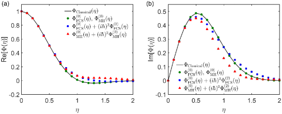
Figure 1: (Color online) Different orders of characteristic functions of work distributions based on the FCS and MH. (a) Real part. (b) Imaginary part. Here $\beta=u=m=\omega=\hbar=1$, $\tau^{\prime}=1$, $\tau=2$. In each figure, there are three sets of points and one curve. The black curve represents the classical characteristic function $\Phi_{\text{Classical}}(\eta)$ [Eq. (36)]. The green circles represent the zeroth order ($\Phi^{(0)}_{\text{FCS}}(\eta)$ and $\Phi^{(0)}_{\text{MH}}(\eta)$) [Eq. (53)]. The blue squares represent the zeroth plus the second orders for the work definition based on the FCS. The red triangles represent the zeroth plus the second orders for the work definition based on the MH.

The detailed calculations of $\Phi^{(2)}_{\text{FCS}}(\eta)$ and $\Phi^{(2)}_{\text{MH}}(\eta)$ are shown in Appendix B. In Fig. 1, we plot the real and the imaginary parts of $\Phi_{\text{Classical}}(\eta)$, $\Phi^{(0)}_{\text{FCS}}(\eta)$, $\Phi^{(0)}_{\text{MH}}(\eta)$, $\Phi^{(0)}_{\text{FCS}}(\eta)+(\mathrm{i}\hbar)^{2}\Phi^{(2)}_{\text{FCS}}(\eta)$, and $\Phi^{(0)}_{\text{MH}}(\eta)+(\mathrm{i}\hbar)^{2}\Phi^{(2)}_{\text{MH}}(\eta)$ of the linearly dragged harmonic oscillator. It is easy to see the quantum-classical correspondence and the differences between $\Phi_{\text{FCS}}(\eta)$ and $\Phi_{\text{MH}}(\eta)$.

IV Discussion and conclusion

IV.1 Generalized Jarzynski equalities for arbitrary initial states with quantum coherence

Based on the FCS and the MH, one can define the quantum fluctuating work for quantum systems with initial coherence. One of the applications of these definitions of quantum fluctuating work is to study the Jarzynski equality for arbitrary initial states. In Ref. Gong and Quan (2015), the Jarzynski equality Jarzynski (1997); Seifert (2012); Jarzynski (2011) is extended to arbitrary initial states in the classical regime. If the initial distribution in the phase space is $p(x,p,0)$, then

$$\left\langle\mathrm{e}^{-\beta\left(W-\Delta F\right)}\right\rangle_{p(x,p,0)}=\iint\mathrm{d}x\mathrm{d}p\ p^{R}(x,-p,\tau)\frac{p(x,p,0)}{p^{eq}(x,p,0)},$$ (56)

where $p^{eq}(x,p,0)$ is the equilibrium distribution at the initial time $t=0$, and $p^{R}(x,-p,\tau)$ is the final distribution of the corresponding time-reversal process Crooks (1999); Jarzynski (2011); Seifert (2012) whose initial state is chosen to be the equilibrium state.

In the quantum regime for isolated quantum systems, if the initial state $\hat{\rho}(0)$ does not have coherence, Eq. (56) can be straightforwardly generalized to the quantum version by adopting the TPM approach:

$$\left\langle\mathrm{e}^{-\beta\left(W-\Delta F\right)}\right\rangle_{\hat{\rho}(0)} = \sum_{n}\rho_{nn}^{R}(\tau)\frac{\rho_{nn}(0)}{\rho_{nn}^{eq}(0)}$$ (57)

$$= \text{Tr}\left[\hat{\rho}(0)\hat{\rho}^{R}(\tau)\left(\hat{\rho}^{eq}(0)\right)^{-1}\right],$$

where $\hat{\rho}^{eq}(0)$ is the equilibrium density matrix at the initial time $t=0$, and $\hat{\rho}^{R}(\tau)$ is the final density matrix of the corresponding time-reversal process whose initial state is chosen to be the equilibrium density matrix. The subscript $nn$ depicts the $n$-th diagonal matrix element.

If the initial state $\hat{\rho}(0)$ has coherence, then according to the work definition based on the FCS [Eq. (4)], we can similarly generalize the Jarzynski equality to arbitrary initial states with quantum coherence:

$$\left\langle\mathrm{e}^{-\beta\left(W-\Delta F\right)}\right\rangle_{\hat{\rho}(0)}=\sum_{m,n}\rho_{mn}^{R}(\tau)\frac{\rho_{nm}(0)}{\sqrt{\rho_{mm}^{eq}(0)\rho_{nn}^{eq}(0)}},$$ (58)

where the subscript $mn$ depicts the matrix element in the $m$-th row and the $n$-th column. For the work definition based on the MH [Eq. (5)], the generalized Jarzynski equality for arbitrary initial states with quantum coherence is Allahverdyan (2014)

$$\left\langle\mathrm{e}^{-\beta\left(W-\Delta F\right)}\right\rangle_{\hat{\rho}(0)}=\text{Re}\ \text{Tr}\left[\hat{\rho}(0)\hat{\rho}^{R}(\tau)\left(\hat{\rho}^{eq}(0)\right)^{-1}\right].$$ (59)

Thus by adopting work definitions based on the FCS and the MH, we extend Jarzynski equality from equilibrium initial states to arbitrary initial states with quantum coherence.

IV.2 Effect of the first projective energy measurement

Quantum coherence of the initial states is the main concern of our current study. We may ask a question: does the quantum-classical correspondence of work distributions still hold if we make a projective energy measurement at the initial time? For initial states without coherence, the answer is yes because the states remain unchanged after the first projective measurement.

For the initial states with quantum coherence, in the energy basis, the off-diagonal elements will be destroyed by the measurement. Initially, $\left[\hat{\rho}(0),\hat{H}(0)\right]\neq 0$. The initial Wigner function of $\hat{\rho}(0)$ is $P(z,0)$. After the projective energy measurement, $\hat{\rho}(0)$ becomes $\hat{\tilde{\rho}}(0)$, and the Wigner function becomes

$$\tilde{P}(r,0)=\frac{1}{2\pi}\int_{0}^{2\pi}\mathrm{d}\theta^{\prime}P(r,\theta^{\prime},0),$$ (60)

where $P(r,\theta,0)$ and $\tilde{P}(r,\theta,0)$ are expressed in the polar coordinate, corresponding to $P(z,0)$ and $\tilde{P}(z,0)$ respectively. The derivation of Eq. (60) is given in Appendix C. As we can see, $\tilde{P}$ is the average of $P$ over the angular coordinate $\theta$, thus $\tilde{P}$ is independent of $\theta$. Since $P(r,\theta,0)$ [Eq. (38)] and $P^{(0)}(r,\theta,0)$ [Eq. (39)] are $\theta$-dependent, we obtain

$$\tilde{P}(z,0) \neq P(z,0),$$ (61)

$$\tilde{P}^{(0)}(z,0) \neq P^{(0)}(z,0).$$ (62)

The change of the initial state due to the first projective energy measurement will influence the work statistics. Thus after the first projective energy measurement, both the initial state and the work statistics will change in all orders of $\hbar$, including the zeroth order.

IV.3 Wigner function and quasi-probability

In quantum mechanics, a point in the phase space is not a proper way to describe the state of the system due to the uncertainty principle. Nevertheless, in order to compare with its classical counterpart, physicists introduced a quasi-probability known as the Wigner function. But this quasi-probability may be negative. The leading order of the Wigner function is equal to the classical distribution in the phase space Wigner (1932), which provides some justification for the concept of the Wigner function as a quasi-probability. Similarly, in quantum thermodynamics, when dealing with quantum systems with initial coherence, it is improper to define quantum fluctuating work along individual stochastic trajectories in the phase space. Nevertheless, physicists introduced the quantum fluctuating work based on the FCS or the MH, but the work distribution may be negative (quasi-probability). We find that the leading order of the work distribution is equal to the classical counterpart, which implies the quantum-classical correspondence of work distributions, and provides some justification for definitions of quantum fluctuating work based on the FCS and the MH.

In summary, in recent years, definitions of quantum fluctuating work based on the FCS and the MH have been proposed for initial states with quantum coherence, and have attracted a lot of attention. But these definitions seem ad hoc. In this article, we study the quantum-classical correspondence of work distributions based on the two definitions. Firstly, for the general cases, we prove that both definitions satisfy the quantum Feynman-Kac formula Kac (1949); Liu (2012); Fei et al. (2018). Using the method of the phase space formulation of quantum mechanics Wigner (1932); Hillery et al. (1984); Polkovnikov (2010); Fei et al. (2018) and $\hbar$ expansion, we prove that the leading order of both work distributions corresponds to its classical counterpart. Corrections proportional to odd orders of $\hbar$ vanish, and corrections proportional to $\hbar^{2}$ are different. Then, as an exactly solvable example, we calculate the leading order and the second order of work distributions of a linearly dragged harmonic oscillator. We use this example to demonstrate the quantum-classical correspondence of work distributions and the quantum corrections. In addition, we discuss the generalized Jarzynski equalities for arbitrary initial states with quantum coherence based on the FCS and the MH. Our work is an extension of previous work for the definition based on the TPM Jarzynski et al. (2015); Zhu et al. (2016); Wang and Quan (2017); Fei et al. (2018); García-Mata et al. (2017); Arrais et al. (2018); García-Mata et al. (2018), and provides some justification for the validity of the definitions of quantum fluctuating work based on the FCS and the MH.

Appendix A Derivation of Eqs. (19) and (45)

Firstly, let us derive Eq. (19). From the initial condition of $\hat{K}(t)$ based on $\Phi_{\text{FCS}}(\eta)$ [Eq. (8)], we obtain the Weyl symbol of the operator $\hat{K}(0)$:

$$K(z,0)=\left[\left\{\mathrm{e}^{\mathrm{i}\frac{\eta}{2}\hat{H}(0)}\right\}_{w}\exp\left(\frac{\mathrm{i}\hbar}{2}\Lambda\right)P(z,0)\right]\exp\left(\frac{\mathrm{i}\hbar}{2}\Lambda\right)\left\{\mathrm{e}^{-\mathrm{i}\frac{\eta}{2}\hat{H}(0)}\right\}_{w}.$$ (63)

We expand $K(z,0)$ in powers of $\hbar$, and we obtain the zeroth order when we take the zeroth order of each term in the Weyl symbol:

$$K^{(0)}(z,0) = \mathrm{e}^{\mathrm{i}\frac{\eta}{2}H(z,0)}P^{(0)}(z,0)\mathrm{e}^{-\mathrm{i}\frac{\eta}{2}H(z,0)}$$ (64)

$$= P^{(0)}(z,0).$$

Since the initial state $P(z,0)$ only contains terms proportional to even orders of $\hbar$ [Eq. (21)], the first order of $K(z,0)$ originating from the two star products $\exp\left(\frac{\mathrm{i}\hbar}{2}\Lambda\right)$ is

$$K^{(1)}(z,0)= \left(\mathrm{e}^{\mathrm{i}\frac{\eta}{2}H(z,0)}\frac{1}{2}\Lambda P^{(0)}(z,0)\right)\mathrm{e}^{-\mathrm{i}\frac{\eta}{2}H(z,0)}$$

$$+\left(\mathrm{e}^{\mathrm{i}\frac{\eta}{2}H(z,0)}P^{(0)}(z,0)\right)\frac{1}{2}\Lambda\mathrm{e}^{-\mathrm{i}\frac{\eta}{2}H(z,0)}$$

$$= \frac{\mathrm{i}\eta}{2}\frac{1}{2}\left[H(z,0)\Lambda P^{(0)}(z,0)-P^{(0)}(z,0)\Lambda H(z,0)\right]$$

$$= \frac{\mathrm{i}\eta}{2}H(z,0)\Lambda P^{(0)}(z,0).$$ (65)

Equations (64) and (65) are Eq. (19).

For the initial condition of $\hat{K}(t)$ based on $\Phi_{\text{MH}}(\eta)$ [Eq. (30)], the Weyl symbol of the operator $\hat{K}(0)$ is

$$K(z,0)=\frac{1}{2}\left[P(z,0)+\left(\left\{\mathrm{e}^{\mathrm{i}\eta\hat{H}(0)}\right\}_{w}\exp\left(\frac{\mathrm{i}\hbar}{2}\Lambda\right)P(z,0)\right)\exp\left(\frac{\mathrm{i}\hbar}{2}\Lambda\right)\left\{\mathrm{e}^{-\mathrm{i}\eta\hat{H}(0)}\right\}_{w}\right].$$ (66)

The zeroth order is

$$K^{(0)}(z,0) = \frac{1}{2}\left[P^{(0)}(z,0)+\mathrm{e}^{\mathrm{i}\eta H(z,0)}P^{(0)}(z,0)\mathrm{e}^{-\mathrm{i}\eta H(z,0)}\right]$$ (67)

$$= P^{(0)}(z,0).$$

Using the conclusion of Eq. (65) , the first order is the same as that based on the FCS:

$$K^{(1)}(z,0) = \frac{1}{2}\left[0+\mathrm{i}\eta H(z,0)\Lambda P^{(0)}(z,0)\right]$$ (68)

$$= \frac{\mathrm{i}\eta}{2}H(z,0)\Lambda P^{(0)}(z,0).$$

Equations (67) and (68) are also Eq. (19).

We would like to emphasize that $K^{(2)}(z,0)$, $K^{(3)}(z,0)$, $\cdots$ based on $\Phi_{\text{FCS}}(\eta)$ and $\Phi_{\text{MH}}(\eta)$ are different [see Eq. (55)].

Then let us derive Eq. (45). From the initial condition of $\hat{M}(t)$ based on $\Phi_{\text{FCS}}(\eta)$ [Eq. (43)], we obtain the Weyl symbol of the operator $\hat{M}(0)$:

$$M(z,0)=\left[\left\{\mathrm{e}^{-\mathrm{i}\frac{\eta}{2}\hat{H}(0)}\right\}_{w}\exp\left(\frac{\mathrm{i}\hbar}{2}\Lambda\right)P(z,0)\right]\exp\left(\frac{\mathrm{i}\hbar}{2}\Lambda\right)\left\{\mathrm{e}^{-\mathrm{i}\frac{\eta}{2}\hat{H}(0)}\right\}_{w}.$$ (69)

The zeroth order is

$$M^{(0)}(z,0)=\mathrm{e}^{-\mathrm{i}\eta H(z,0)}P^{(0)}(z,0).$$ (70)

The first order originating from the two star products $\exp\left(\frac{\mathrm{i}\hbar}{2}\Lambda\right)$ is

$$M^{(1)}(z,0)= \left(\mathrm{e}^{-\mathrm{i}\frac{\eta}{2}H(z,0)}\frac{1}{2}\Lambda P^{(0)}(z,0)\right)\mathrm{e}^{-\mathrm{i}\frac{\eta}{2}H(z,0)}$$

$$+\left(\mathrm{e}^{-\mathrm{i}\frac{\eta}{2}H(z,0)}P^{(0)}(z,0)\right)\frac{1}{2}\Lambda\mathrm{e}^{-\mathrm{i}\frac{\eta}{2}H(z,0)}$$

$$= -\frac{\mathrm{i}\eta}{2}\mathrm{e}^{-\mathrm{i}\eta H(z,0)}\times$$

$$\frac{1}{2}\left[H(z,0)\Lambda P^{(0)}(z,0)+P^{(0)}(z,0)\Lambda H(z,0)\right]$$

$$= 0.$$ (71)

Thus the first order vanishes. Similarly, the terms in $M(z,0)$ proportional to odd orders of $\hbar$ vanish.

For the initial condition of $\hat{M}(t)$ based on $\Phi_{\text{MH}}(\eta)$ [Eq. (52)], the Weyl symbol of the operator $\hat{M}(0)$ is

$$M(z,0) = \frac{1}{2}\left[\left\{\mathrm{e}^{-\mathrm{i}\eta\hat{H}(0)}\right\}_{w}\exp\left(\frac{\mathrm{i}\hbar}{2}\Lambda\right)P(z,0)+P(z,0)\exp\left(\frac{\mathrm{i}\hbar}{2}\Lambda\right)\left\{\mathrm{e}^{-\mathrm{i}\eta\hat{H}(0)}\right\}_{w}\right]$$ (72)

$$= \left\{\mathrm{e}^{-\mathrm{i}\eta\hat{H}(0)}\right\}_{w}\cos\left(\frac{\hbar}{2}\Lambda\right)P(z,0).$$

The zeroth order is the same as Eq. (70). The terms proportional to odd orders of $\hbar$ vanish because $\left\{\mathrm{e}^{-\mathrm{i}\eta\hat{H}(0)}\right\}_{w}$, $\cos\left(\frac{\hbar}{2}\Lambda\right)$, and $P(z,0)$ only contain terms proportional to even orders of $\hbar$. Thus for both work definitions based on the FCS and the MH, $M(z,0)$ can be expanded in the form of Eq. (45).

We would like to emphasize that $M^{(2)}(z,0)$, $M^{(4)}(z,0)$, $\cdots$ based on $\Phi_{\text{FCS}}(\eta)$ and $\Phi_{\text{MH}}(\eta)$ are different [see Eq. (55)].

Appendix B Calculation of $\Phi^{(0)}(\eta)$ and $\Phi^{(2)}(\eta)$ for the linearly dragged harmonic oscillator

From Eq. (44), we know that both $M^{(0)}(z,t)$ and $M^{(2)}(z,t)$ satisfy the classical Liouville equation. That is, the trajectory in the phase space satisfies Newton’s equation. For the Hamiltonian of the linearly dragged harmonic oscillator [Eq. (31)], we obtain

$$\left\{\begin{aligned} &x(t)=x(0)\cos\omega t+\frac{p(0)}{m\omega}\sin\omega t+ut-\frac{u}{\omega}\sin\omega t,\\ &p(t)=-x(0)m\omega\sin\omega t+p(0)\cos\omega t+mu(1-\cos\omega t).\end{aligned}\right.$$ (73)

This is a mapping from $\left(x(0),p(0)\right)$ to $\left(x(t),p(t)\right)$, and we denote it as

$$z(t)=\psi_{t}\left(z(0),0\right).$$ (74)

The inverse mapping is

$$z(0)=\psi^{-1}_{0}\left(z(t),t\right).$$ (75)

More specifically,

$$\left\{\begin{aligned} &x(0)=x(t)\cos\omega t-\frac{p(t)}{m\omega}\sin\omega t-u\left(t\cos\omega t-\frac{1}{\omega}\sin\omega t\right),\\ &p(0)=x(t)m\omega\sin\omega t+p(t)\cos\omega t-mu(\omega t\sin\omega t+\cos\omega t-1).\end{aligned}\right.$$ (76)

Since in the isolated system, the Newton’s trajectory starting from one phase space point is unique, the mapping [Eq. (75)] is one-to-one. From Liouville’s theorem, we obtain

$$M^{(0)}(z,\tau)=M^{(0)}(\psi^{-1}_{0}(z,\tau),0).$$ (77)

By utilizing Eqs. (39), (45) and (47), we obtain

$$\Phi^{(0)}(\eta) = \int_{-\infty}^{+\infty}\mathrm{d}z\ \mathrm{e}^{\mathrm{i}\eta H(z,\tau)}M^{(0)}(z,\tau)$$ (78)

$$= \int_{-\infty}^{+\infty}\mathrm{d}z\ \mathrm{e}^{\mathrm{i}\eta H(z,\tau)}\mathrm{e}^{-\mathrm{i}\eta H(\psi^{-1}_{0}(z,\tau),0)}P^{(0)}(\psi^{-1}_{0}(z,\tau),0)$$

$$= \exp\left\{mu^{2}\left[\mathrm{i}\eta\left(\cos\omega\tau^{\prime}-\cos\omega(\tau^{\prime}+\tau)\right)-\frac{\eta^{2}}{\beta}\left(1-\cos\omega\tau\right)\right]\right\}.$$

The derivation from the second line to the last line is not shown here since the integrals are all Gaussian. Equation (78) is Eq. (49), which is identical to the classical characteristic function of work $\Phi_{\text{Classical}}(\eta)$ [Eq. (36)].

Similarly, for the second order, we also have

$$M^{(2)}(z,\tau)=M^{(2)}(\psi^{-1}_{0}(z,\tau),0).$$ (79)

From Eq. (46), we obtain that both $\left\{\mathrm{e}^{\mathrm{i}\eta\hat{H}(\tau)}\right\}_{w}^{(2)}$ and $M^{(2)}(z,\tau)$ contribute to $\Phi^{(2)}(\eta)$:

$$\Phi^{(2)}(\eta) = \int_{-\infty}^{+\infty}\mathrm{d}z\ \left[\left\{\mathrm{e}^{\mathrm{i}\eta\hat{H}(\tau)}\right\}_{w}^{(2)}M^{(0)}(z,\tau)+\mathrm{e}^{\mathrm{i}\eta H(z,\tau)}M^{(2)}(z,\tau)\right]$$ (80)

$$= \int_{-\infty}^{+\infty}\mathrm{d}z\ \left[\mathrm{e}^{\mathrm{i}\eta H(z,\tau)}f(-\mathrm{i}\eta,z,\tau)\mathrm{e}^{-\mathrm{i}\eta H(\psi^{-1}_{0}(z,\tau),0)}P^{(0)}(\psi^{-1}_{0}(z,\tau),0)+\mathrm{e}^{\mathrm{i}\eta H(z,\tau)}M^{(2)}(\psi^{-1}_{0}(z,\tau),0)\right],$$

where we have used Eqs. (14) and (15). $M^{(2)}(z,0)$ can be calculated according to Eq. (69) (FCS) and Eq. (72) (MH), respectively. The analytical form of Eq. (80) is too complicated to show here, and we numerically calculate it as a function of $\eta$. The results are shown in Fig. 1.

Appendix C Derivation of Eq. (60)

For convenience, we set $m=\omega=1$ in this section. As we know, after the first projective measurement, only the diagonal elements survive. The $n$-th diagonal element

$$p_{n} = \text{Tr}\left[\hat{\rho}(0)\left|n\right\rangle\left\langle n\right|\right]$$ (81)

$$= \iint\mathrm{d}x\mathrm{d}p\ P(x,p,0)F_{n}(x,p),$$

where $F_{n}(x,p)$ is the Wigner function of the Fock state $\left|n\right\rangle\left\langle n\right|$ Barnett and Radmore (2002):

$$F_{n}(x,p)=2(-1)^{n}\mathrm{e}^{-2\left|\alpha\right|^{2}}L_{n}(4\left|\alpha\right|^{2}),$$ (82)

where

$$\left|\alpha\right|^{2}=\frac{1}{2\hbar}\left(x^{2}+p^{2}\right),$$ (83)

and $L_{n}(x)$ is the Laguerre polynomials:

$$L_{n}(x)=\frac{\mathrm{e}^{x}}{n!}\frac{\mathrm{d}^{n}}{\mathrm{d}x^{n}}\left(\mathrm{e}^{-x}x^{n}\right).$$ (84)

After the projective measurement, the state becomes

$$\hat{\tilde{\rho}}(0)=\sum_{n=0}^{\infty}p_{n}\left|n\right\rangle\left\langle n\right|.$$ (85)

Reformulating Eq. (85) in the Weyl-Wigner representation, the Wigner function of $\hat{\tilde{\rho}}(0)$ can be written as

$$\tilde{P}(x,p,0) = \frac{1}{2\pi\hbar}\sum_{n=0}^{\infty}p_{n}F_{n}(x,p)$$ (86)

$$= \frac{1}{2\pi\hbar}\sum_{n=0}^{\infty}\left[\iint\mathrm{d}x^{\prime}\mathrm{d}p^{\prime}\ P(x^{\prime},p^{\prime},0)F_{n}(x^{\prime},p^{\prime})\right]F_{n}(x,p)$$

$$= \frac{2}{\pi\hbar}\iint\mathrm{d}x^{\prime}\mathrm{d}p^{\prime}\ P(x^{\prime},p^{\prime},0)\mathrm{e}^{-\frac{1}{\hbar}\left(x^{2}+p^{2}+x^{\prime 2}+p^{\prime 2}\right)}\sum_{n=0}^{\infty}L_{n}\left(\frac{2}{\hbar}\left(x^{2}+p^{2}\right)\right)L_{n}\left(\frac{2}{\hbar}\left(x^{\prime 2}+p^{\prime 2}\right)\right).$$

Using the identity of the Laguerre polynomials Barnett and Radmore (2002)

$$\sum_{n=0}^{\infty}L_{n}(x)L_{n}(y)=\mathrm{e}^{\frac{x+y}{2}}\delta(x-y),$$ (87)

and converting Eq. (86) into the polar coordinate, we obtain

$$\tilde{P}(r,\theta,0) = \frac{2}{\pi\hbar}\int_{0}^{\infty}r^{\prime}\mathrm{d}r^{\prime}\int_{0}^{2\pi}\mathrm{d}\theta^{\prime}P(r^{\prime},\theta^{\prime},0)\delta\left(\frac{2}{\hbar}\left(r^{2}-r^{\prime 2}\right)\right)$$ (88)

$$= \frac{1}{2\pi}\int_{0}^{2\pi}\mathrm{d}\theta^{\prime}P(r,\theta^{\prime},0).$$

This is Eq. (60) (the r.h.s. of Eq. (88) is independent of $\theta$).

References

- Jarzynski (2011) C. Jarzynski, Annu. Rev. Condens. Matter Phys. 2, 329 (2011).
- Seifert (2012) U. Seifert, Reports on Progress in Physics 75, 126001 (2012).
- Sekimoto (1998) K. Sekimoto, Progress of Theoretical Physics Supplement 130, 17 (1998).
- Sekimoto (2010) K. Sekimoto, Stochastic Energetics, Lecture Notes in Physics, Vol. 799 (Springer-Verlag, Berlin, 2010).
- Li et al. (2010) T. Li, S. Kheifets, D. Medellin, and M. G. Raizen, Science 328, 1673 (2010).
- Martínez et al. (2016) I. A. Martínez, É. Roldán, L. Dinis, D. Petrov, J. M. R. Parrondo, and R. A. Rica, Nature physics 12, 67 (2016).
- Bang et al. (2018) J. Bang, R. Pan, T. M. Hoang, J. Ahn, C. Jarzynski, H. T. Quan, and T. Li, New Journal of Physics 20, 103032 (2018).
- Jarzynski (1997) C. Jarzynski, Physical Review Letters 78, 2690 (1997).
- Crooks (1999) G. E. Crooks, Physical Review E 60, 2721 (1999).
- Seifert (2005) U. Seifert, Physical Review Letters 95, 040602 (2005).
- Hummer and Szabo (2001) G. Hummer and A. Szabo, Proc. Natl. Acad. Sci. 98, 3658 (2001).
- Kawai et al. (2007) R. Kawai, J. M. R. Parrondo, and C. van den Broeck, Phys. Rev. Lett. 98, 080602 (2007).
- Esposito and van den Broeck (2010) M. Esposito and C. van den Broeck, Phys. Rev. Lett. 104, 090601 (2010).
- Gong and Quan (2015) Z. Gong and H. T. Quan, Physical Review E 92, 012131 (2015).
- Liphardt et al. (2002) J. Liphardt, S. Dumont, S. B. Smith, I. Tinoco, and C. Bustamante, Science 296, 1832 (2002).
- Collin et al. (2005) D. Collin, F. Ritort, C. Jarzynski, S. B. Smith, I. Tinoco, and C. Bustamante, Nature (London) 437, 231 (2005).
- Douarche et al. (2006) F. Douarche, S. Joubaud, N. B. Garnier, A. Petrosyan, and S. Ciliberto, Physical Review Letters 97, 140603 (2006).
- Junier et al. (2009) I. Junier, A. Mossa, M. Manosas, and F. Ritort, Physical Review Letters 102, 070602 (2009).
- Toyabe et al. (2010) S. Toyabe, T. Sagawa, M. Ueda, E. Muneyuki, and M. Sano, Nature physics 6, 988 (2010).
- Pekola (2015) J. P. Pekola, Nature Phys. 11, 118 (2015).
- Hoang et al. (2018) T. M. Hoang, R. Pan, J. Ahn, J. Bang, H. T. Quan, and T. Li, Physical Review Letters 120, 080602 (2018).
- Talkner and Hänggi (2016) P. Talkner and P. Hänggi, Physical Review E 93, 022131 (2016).
- Funo and Quan (2018a) K. Funo and H. T. Quan, Physical Review Letters 121, 040602 (2018a).
- Funo and Quan (2018b) K. Funo and H. T. Quan, Phys. Rev. E 98, 012113 (2018b).
- Kurchan (2000) J. Kurchan, arXiv:cond-mat/0007360 (2000).
- Tasaki (2000) H. Tasaki, arXiv:cond-mat/0009244 (2000).
- Talkner et al. (2007) P. Talkner, E. Lutz, and P. Hänggi, Physical Review E 75, 050102 (2007).
- Brandner and Seifert (2016) K. Brandner and U. Seifert, Phys. Rev. E 93, 062134 (2016).
- Suomela et al. (2016) S. Suomela, A. Kutvonen, and T. Ala-Nissila, Phys. Rev. E 93, 062106 (2016).
- Liu (2016) F. Liu, Phys. Rev. E 93, 012127 (2016).
- Wang (2018) W.-g. Wang, Phys. Rev. E 97, 012128 (2018).
- Liu and Xi (2016) F. Liu and J. Xi, Phys. Rev. E 94, 062133 (2016).
- Rogers (2017) D. M. Rogers, Phys. Rev. E 95, 012149 (2017).
- Aurell (2018) E. Aurell, Phys. Rev. E 97, 062117 (2018).
- Sampaio et al. (2016) R. Sampaio, S. Suomela, and T. Ala-Nissila, Phys. Rev. E 94, 062122 (2016).
- Jaramillo et al. (2017) J. D. Jaramillo, J. Deng, and J. Gong, Phys. Rev. E 96, 042119 (2017).
- Gong et al. (2016) Z. Gong, Y. Ashida, and M. Ueda, Phys. Rev. A 94, 012107 (2016).
- Talarico et al. (2016) M. A. A. Talarico, P. B. Monteiro, E. C. Mattei, E. I. Duzzioni, P. H. Souto Ribeiro, and L. C. Céleri, Phys. Rev. A 94, 042305 (2016).
- Bartolotta and Deffner (2018) A. Bartolotta and S. Deffner, Phys. Rev. X 8, 011033 (2018).
- Silveri et al. (2017) M. Silveri, J. Tuorila, E. Thuneberg, and G. Paraoanu, Reports on Progress in Physics 80, 056002 (2017).
- Frenzel et al. (2016) M. F. Frenzel, D. Jennings, and T. Rudolph, New Journal of Physics 18, 023037 (2016).
- Guarnieri et al. (2018) G. Guarnieri, N. H. Y. Ng, K. Modi, J. Eisert, M. Paternostro, and J. Goold, arXiv:1804.09962 (2018).
- Kwon and Kim (2018) H. Kwon and M. Kim, arXiv:1810.03150 (2018).
- Peng and Fan (2017) Y. Peng and H. Fan, arXiv:1708.08214 (2017).
- Strasberg (2018) P. Strasberg, arXiv:1810.00698 (2018).
- Goold et al. (2016) J. Goold, M. Huber, A. Riera, L. del Rio, and P. Skrzypczyk, Journal of Physics A: Mathematical and Theoretical 49, 143001 (2016).
- Huber et al. (2008) G. Huber, F. Schmidt-Kaler, S. Deffner, and E. Lutz, Phys. Rev. Lett. 101, 070403 (2008).
- Batalhão et al. (2014) T. B. Batalhão, A. M. Souza, L. Mazzola, R. Auccaise, R. S. Sarthour, I. S. Oliveira, J. Goold, G. De Chiara, M. Paternostro, and R. M. Serra, Phys. Rev. Lett. 113, 140601 (2014).
- An et al. (2015) S. An, J.-N. Zhang, M. Um, D. Lv, Y. Lu, J. Zhang, Z.-Q. Yin, H. T. Quan, and K. Kim, Nature Physics 11, 193 (2015).
- Jarzynski et al. (2015) C. Jarzynski, H. T. Quan, and S. Rahav, Physical Review X 5, 031038 (2015).
- Zhu et al. (2016) L. Zhu, Z. Gong, B. Wu, and H. T. Quan, Physical Review E 93, 062108 (2016).
- Wang and Quan (2017) Q. Wang and H. T. Quan, Phys. Rev. E 95, 032113 (2017).
- Fei et al. (2018) Z. Fei, H. T. Quan, and F. Liu, Physical Review E 98, 012132 (2018).
- García-Mata et al. (2017) I. García-Mata, A. J. Roncaglia, and D. A. Wisniacki, Phys. Rev. E 95, 050102 (2017).
- Arrais et al. (2018) E. G. Arrais, D. A. Wisniacki, L. C. Céleri, N. G. de Almeida, A. J. Roncaglia, and F. Toscano, Phys. Rev. E 98, 012106 (2018).
- García-Mata et al. (2018) I. García-Mata, A. J. Roncaglia, and D. A. Wisniacki, EPL (Europhysics Letters) 120, 30002 (2018).
- Perarnau-Llobet et al. (2017) M. Perarnau-Llobet, E. Bäumer, K. V. Hovhannisyan, M. Huber, and A. Acin, Physical Review Letters 118, 070601 (2017).
- Lostaglio (2018) M. Lostaglio, Physical Review Letters 120, 040602 (2018).
- Bäumer et al. (2018) E. Bäumer, M. Lostaglio, M. Perarnau-Llobet, and R. Sampaio, arXiv:1805.10096 (2018).
- Allahverdyan (2014) A. Allahverdyan, Physical Review E 90, 032137 (2014).
- Solinas and Gasparinetti (2015) P. Solinas and S. Gasparinetti, Physical Review E 92, 042150 (2015).
- Hofer and Clerk (2016) P. P. Hofer and A. A. Clerk, Physical Review Letters 116, 013603 (2016).
- Solinas and Gasparinetti (2016) P. Solinas and S. Gasparinetti, Physical Review A 94, 052103 (2016).
- Solinas et al. (2017) P. Solinas, H. Miller, and J. Anders, Physical Review A 96, 052115 (2017).
- Miller and Anders (2017) H. J. Miller and J. Anders, New Journal of Physics 19, 062001 (2017).
- Miller and Anders (2018) H. J. Miller and J. Anders, Entropy 20, 200 (2018).
- Åberg (2018) J. Åberg, Physical Review X 8, 011019 (2018).
- Sampaio et al. (2018) R. Sampaio, S. Suomela, T. Ala-Nissila, J. Anders, and T. Philbin, Physical Review A 97, 012131 (2018).
- Francica et al. (2017) G. Francica, J. Goold, and F. Plastina, arXiv:1707.06950 (2017).
- Xu et al. (2018) B.-M. Xu, J. Zou, L.-S. Guo, and X.-M. Kong, Physical Review A 97, 052122 (2018).
- Xu et al. (2019) B.-M. Xu, Z.-C. Tu, J. Zou, and J. Wang, arXiv:1903.01064 (2019).
- Wu et al. (2019) K.-D. Wu, Y. Yuan, G.-Y. Xiang, C.-F. Li, G.-C. Guo, and M. Perarnau-Llobet, Science advances 5, eaav4944 (2019).
- Allahverdyan and Nieuwenhuizen (2005) A. Allahverdyan and T. M. Nieuwenhuizen, Physical Review E 71, 066102 (2005).
- Margenau and Hill (1961) H. Margenau and R. N. Hill, Progress of Theoretical Physics 26, 722 (1961).
- Nazarov and Kindermann (2003) Y. V. Nazarov and M. Kindermann, The European Physical Journal B-Condensed Matter and Complex Systems 35, 413 (2003).
- Johansen (2007) L. M. Johansen, Physical Review A 76, 012119 (2007).
- Lundeen and Bamber (2012) J. S. Lundeen and C. Bamber, Physical Review Letters 108, 070402 (2012).
- Wigner (1932) E. Wigner, Phys. Rev. 40, 749 (1932).
- Hillery et al. (1984) M. Hillery, R. F. O’Connell, M. O. Scully, and E. P. Wigner, Physics reports 106, 121 (1984).
- Polkovnikov (2010) A. Polkovnikov, Annals of Physics 325, 1790 (2010).
- Kac (1949) M. Kac, Transactions of the American Mathematical Society 65, 1 (1949).
- Liu (2012) F. Liu, Physical Review E 86, 010103 (2012).
- Talkner et al. (2008) P. Talkner, P. S. Burada, and P. Hänggi, Physical Review E 78, 011115 (2008).
- Deffner and Lutz (2008) S. Deffner and E. Lutz, Physical Review E 77, 021128 (2008).
- Pan et al. (2018) R. Pan, T. M. Hoang, Z. Fei, T. Qiu, J. Ahn, T. Li, and H. T. Quan, Physical Review E 98, 052105 (2018).
- Barnett and Radmore (2002) S. Barnett and P. M. Radmore, Methods in theoretical quantum optics, Vol. 15 (Oxford University Press, 2002).