Compressed sensing reconstruction using Expectation Propagation

Abstract

Many interesting problems in fields ranging from telecommunications to computational biology can be formalized in terms of large underdetermined systems of linear equations with additional constraints or regularizers. One of the most studied ones, the Compressed Sensing problem (CS), consists in finding the solution with the smallest number of non-zero components of a given system of linear equations $\bm{y}=\mathbf{F}{\bm{w}}$ for known measurement vector $\bm{y}$ and sensing matrix $\mathbf{F}$. Here, we will address the compressed sensing problem within a Bayesian inference framework where the sparsity constraint is remapped into a singular prior distribution (called Spike-and-Slab or Bernoulli-Gauss). Solution to the problem is attempted through the computation of marginal distributions via Expectation Propagation (EP), an iterative computational scheme originally developed in Statistical Physics. We will show that this strategy is more accurate for statistically correlated measurement matrices. For computational strategies based on the Bayesian framework such as variants of Belief Propagation, this is to be expected, as they implicitly rely on the hypothesis of statistical independence among the entries of the sensing matrix. Perhaps surprisingly, the method outperforms uniformly also all the other state-of-the-art methods in our tests.

1 Introduction

The problem of Compressed Sensing (CS) [1, 2, 3] has led to significant developments in the field of sparse approximation and representation [4], together with the more traditional framework of optimal signal processing [4, 5].

In general, CS deals with the reconstruction of a sparse $N-$dimensional signal from $M$, often noisy, measurements. In this context, a sparse signal is characterized by a large (possibly the largest) number of components equal to zero. In practical cases, the regime of interest is given by the $M\ll N$, $K\ll N$ limit of the problem, where $K$ is the number of non-zero components. A brute-force exhaustive search of the $K-$dimensional minimal support of the $N-$dimensional signal would lead to an exponential explosion in the search space as there are $N\choose K$ possible base supports to be explored. In the noiseless limit of CS, even if the $K$-dimensional minimal base were given, at least $M=K$ measurements are necessary to uniquely identify the solution.

CS can be easily formulated: let $\bm{w}\in{\mathbb{R}}^{N}$ be compressed into a vector $\bm{y}\in{\mathbb{R}}^{M}$ (from now on we will assume $M<N$) through a linear transformation:

$$\bm{y}=\mathbf{F}{\bm{w}},$$ (1)

where $\mathbf{F}\in{\mathbb{R}}^{M\times N}$ is a linear operator of maximal rank often referred to as the measurement or sensing matrix. The problem is to determine the vector $\bm{w}$ from the knowledge of the measurement matrix $\mathbf{F}$ and of the compressed vector $\bm{y}$.

The relevance of CS in statistical physics stems from the link with the statistical mechanics of disordered systems, in analogy with many other combinatorial optimization problems [6, 7, 8]. In particular CS is an optimization problem with quenched disorder (the measurement matrix) and, as such, it is amenable to analytic treatment using replica theory [9] as developed in the field of spin-glasses [10].

From equation (1), it is clear that, as long as $M<N$, there are infinitely many solutions to the system of equations. However, if one imposes the supplementary condition on the sparsity of the signal $\bm{w}$, solving the problem may still lead to a unique retrieved signal. Thus, a problem in CS is to determine the set of conditions under which it is possible to find a solution of equation (1) that is as sparse as possible. A practical way to enforce sparsity is through the minimization of the $L_{p}$-norm of the $\bm{w}$ vector in the space of solutions which is defined in equation (1). A particularly successful line of research has been pursued through the minimization of the $L_{1}$ norm [1, 11, 3, 12, 2, 13, 9], for which the following prediction was obtained in the case of independent and identically distributed (i.i.d.) random Gaussian measurement matrices: in the large $N$ limit, there is a non-trivial region $\rho=K/N$, $\alpha=M/N$ where an exact reconstruction of the original signal is indeed possible. The parameters $\rho$ and $\alpha$ that characterize the signal are called the signal density and the measurement rate, respectively.

However, in many applications, the sensing matrix may not be random [14] or the i.i.d. assumption might not hold and, in these cases, several algorithms could fail to decode the signal. Examples of deterministic matrices include chirp sensing matrices [15], which have been applied to image reconstruction [16], and second-order Reed-Muller matrices [17], whereas examples of correlated random matrices include random partial Fourier matrices [18, 19], which are encountered in MRI [20] as well as in other applications [21, 22], and partial random circulant and Toeplitz matrices [23], which arise in the presence of convolutions.

Our approach here, is to treat CS as a Bayesian inference problem, i.e. we focus our attention on determining the probability of observing, a posteriori, the signal $\bm{w}$ when we have observed a set of measurements $\bm{y}$ and given the sensing matrix $\mathbf{F}$. While equation (1) is easily cast in a Gaussian-like likelihood function, the prior over the variables $\bm{w}$, enforcing the sparsity constraint, plays a key role on the goodness of the solution and on the complexity of the problem. A prior that corresponds to the minimization of a $L_{p}$ norm, with $p={1,2}$, allows an easy marginalization of the corresponding posterior probability with the drawback of softening the sparsity requirement. Similarly to [9, 24, 25], we consider the so-called spike-and-slab prior [26] which is understood as the minimization of the $L_{0}$ norm of the vector $\bm{w}$. The posterior distribution results to be intractable in practice and thus some approximations need to be sought.

Almost twenty years ago Expectation Propagation (EP), an iterative scheme to approximate intractable distributions, has been introduced first in the field of statistical physics [27, 28] and shortly after in the field of theoretical computer science [29]. Recently, EP inspired inference strategies – similar to the one we present here – have been proposed to solve other underdetermined linear constraint problems such as the problem of sampling solutions from the reconstruction of large scale metabolic networks [30] and of tomographic images [31]. Here we propose an efficient and accurate EP-based reconstruction strategy for CS which, moreover, does not require i.i.d. measurement matrices.

Other attempts to solve sparse linear models using the EP approximation can be found in [32] – where the authors use a similar EP implementation to the one we adopt here and make use of a Laplace prior – and in [33] – where, in addition to the spike-and-slab, a Bernoulli prior on the components of the signal is introduced and the EP update scheme involves only three approximating factors of the original posterior distribution.

All these approaches have the same computational complexity, which is dominated by a single matrix inversion per EP cycle. In our implementation, we integrate the inference of the signal with a variational learning of the density parameter of the spike-and-slab prior. Besides, we show in A that the original EP scheme is equivalent to an alternative formulation of the EP update equations that takes into account the linear constraints (1) exactly. This implementation has the advantage of reducing the size of the matrix to be inverted, thus decreasing the computing time. Throughout the work presented in this paper, we have numerically checked that both procedures can be used interchangeably in the case of noiseless measurements, as they lead to the same results.

In conclusion, we believe that our EP algorithm shows some original features that have not been proposed by other methods, namely: (i) the quality of EP reconstruction on correlated measurement matrices is the same as in the case of uncorrelated measurements whereas all other methods we tested fail; (ii) to reconstruct signals in the noiseless case, we introduced an EP formulation performing analytically the zero temperature limit; (iii) we learn the density parameter of the spike and slab prior from the data by minimizing iteratively the EP free energy.

The outline is as follows: we introduce the EP approach to CS and set the basic notations in section 2, we show a thorough comparison with other state of the art algorithms in section 3 and, finally, we present our conclusions in section 4.

2 Expectation Propagation

In this section we introduce the so-called finite temperature formulation of EP, where we allow the measurement vector $\bm{y}$ to be noisy. We consider the undersampling regime $M<N$, although there is no technical limitation in considering the $M\geq N$ case. The linear constraints in equation (1) can be alternatively mapped into a minimization problem of the following quadratic form:

$$E(\bm{w})=\frac{1}{2}\left\|{\bm{y}}-\mathbf{F}\bm{w}\right\|_{2}:=\frac{1}{2}\left({\bm{y}}-\mathbf{F}\bm{w}\right)^{T}\cdot\left({\bm{y}}-\mathbf{F}\bm{w}\right),$$ (2)

From a Bayesian perspective, the probability of observing the vector ${\bm{y}}$ given the matrix $\mathbf{F}$ and the vector ${\bm{w}}$ is:

$$P({\bm{y}}|\mathbf{F},{\bm{w}}) = \left(\frac{\beta}{2\pi}\right)^{\frac{M}{2}}e^{-\beta E(\bm{w})},$$ (3)

where we introduced a fictitious inverse temperature $\beta$ that we can take as large as we wish in order to enforce the linear bounds expressed by equation (1). Alternatively we can interpret equation (3) as the probability of observing an additive noise vector $\bm{y}-\mathbf{F}\bm{w}$ whose elements are distributed according to a Gaussian density of zero mean and variance $\beta^{-1}$. The posterior distribution for the vector ${\bm{w}}$ reads:

$$P\left(\bm{w}|\mathbf{F},\bm{y}\right) = \frac{P\left(\bm{y}|\mathbf{F},{\bm{w}}\right)P\left(\bm{w}\right)}{P\left({\bm{y}}\right)}=\frac{1}{Z_{P}}e^{-\beta\frac{\left({\bm{y}}-\mathbf{F}\bm{w}\right)^{T}\cdot\left({\bm{y}}-\mathbf{F}\bm{w}\right)}{2}}\prod_{i=1}^{N}\psi_{i}(w_{i}),$$ (4)

where in the last step we restricted the structure of the prior $P({\bm{w}}):=\prod_{i=1}^{N}\psi_{i}(w_{i})$ to a factorized form, although more general structures can be considered, e.g. as in [34]. In this work, we have considered the so-called spike-and-slab prior [26]:

$$\psi(w_{i})=(1-\rho)\delta(w_{i})+\frac{\rho}{\sqrt{2\pi\lambda}}e^{-\frac{w_{i}^{2}}{2\lambda}},$$ (5)

where $\delta$ denotes the Dirac delta function, in order to model any prior knowledge about the sparsity of the signal.

We seek a solution vector $\hat{\bm{w}}$ whose components are the first moments of the marginal densities of equation (4). Contrarily to the maximum a posteriori estimate, it can be proven that this strategy minimizes the mean squared error between the true and the recovered signal. Unfortunately, due to the non-convex nature of the spike-and-slab prior, there exists no technique able to perform the marginalization of the posterior probability in equation (4). In the following we introduce the EP approximation scheme which relies on an adaptive Gaussian approximation of the marginal probabilities of interest.

2.1 The approximate posterior distribution

EP [29] is an efficient approximation to compute posterior probabilities. EP was first introduced as an improved mean-field method [27, 28] and further developed in the framework of Bayesian inference problems in the seminal work of Minka [29]. The approximated distribution consists in substituting the typically analytically intractable $\psi_{i}$ priors with univariate Gaussian distributions $\phi_{i}(w_{i})={\cal N}(w_{i};a_{i},d_{i})$ of mean $a_{i}$ and variance $d_{i}.$ The approximated posterior thus reads:

$$Q({\bm{w}}|\mathbf{F},{\bm{y}}) = \frac{1}{Z_{Q}}e^{-\beta\frac{\left({\bm{y}}-\mathbf{F}\bm{w}\right)^{T}\cdot\left({\bm{y}}-\mathbf{F}\bm{w}\right)}{2}}\prod_{i=1}^{N}\phi_{i}(w_{i})$$ (6)

$$:= \frac{1}{Z_{Q}}e^{-\frac{1}{2}({\bm{w}}-\bar{{\bm{w}}})^{T}\bm{\Sigma}^{-1}({\bm{w}}-\bar{{\bm{w}}})},$$

where:

$$Z_{Q}=\left(2\pi\right)^{\frac{N}{2}}\left(\det\bm{\Sigma}\right)^{\frac{1}{2}},$$ (7)

$$\bm{\Sigma}^{-1}:=\beta\mathbf{F}^{T}\mathbf{F}+\bm{D},\quad\bar{{\bm{w}}}:=\bm{\Sigma}(\beta\mathbf{F}^{T}{\bm{y}}+\bm{D}{\bm{a}}),$$ (8)

and $\bm{D}$ is a diagonal matrix having diagonal elements $d_{1}^{-1},\dots,d_{N}^{-1}$. We now need a way to fix the parameters ${\bm{a},\bm{d}}$ of the prior. To do so, we focus on the $n^{th}$ variable $w_{n}$ (with $1\leq n\leq N$), and in particular on its approximated prior $\phi_{n}$. We can define the tilted distribution $Q^{(n)}$ as:

$$Q^{(n)}({\bm{w}}|\mathbf{F},{\bm{y}}) := \frac{1}{Z_{Q^{(n)}}}e^{-\beta\frac{\left({\bm{y}}-\mathbf{F}\bm{w}\right)^{T}\cdot\left({\bm{y}}-\mathbf{F}\bm{w}\right)}{2}}\psi_{n}(w_{n})\prod_{l\neq n}\phi_{l}(w_{l};a_{l,}d_{l})$$ (9)

$$= \frac{1}{Z_{{Q}^{(n)}}}e^{-\frac{1}{2}({\bm{w}}-\bar{{\bm{w}}}_{(n)})^{T}\Sigma_{(n)}^{-1}({\bm{w}}-\bar{{\bm{w}}}_{(n)})}\psi_{n}(w_{n}),$$

where:

$$\bm{\Sigma}_{(n)}^{-1}=\beta\mathbf{F}^{T}\mathbf{F}+\bm{D}_{(n)},\quad\bar{{\bm{w}}}_{(n)}=\bm{\Sigma}_{(n)}\left(\beta\mathbf{F}^{T}{\bm{\bm{y}}}+\bm{D}_{(n)}\bm{a}\right),$$ (10)

and, in analogy with equation (8), $\bm{D}_{(n)}$ is a diagonal matrix of elements $d_{m}^{-1}$ for all diagonal elements $m\neq n$ and zero for $m=n$. The tilted distribution differs from the approximated posterior $Q$ as it contains the original prior $\psi_{n}$ instead of the $n$-th approximated prior $\phi_{n}$. Intuitively, we expect that the ${n}$-th tilted distribution provides a better approximation of the expectation values related to the $n$-th variable than the multivariate Gaussian approximation. From a computational point of view, the presence of a single intractable prior in the tilted distribution does not prejudice the efficiency of the algorithm.

A natural way of fixing the optimal $\bm{a},\bm{d}$ parameters consists in requiring the approximated $Q$ distribution to be as similar as possible to the tilted distribution $Q^{(n)}.$ To do so, we minimize the Kullback-Leibler divergence $D_{KL}\left(Q^{(n)}||Q\right)$. Perhaps not surprisingly, this procedure is equivalent to equating the first two moments of the two distributions:

$$\left\langle w_{n}\right\rangle_{Q^{\left(n\right)}} = \left\langle w_{n}\right\rangle_{Q},\quad\left\langle w_{n}^{2}\right\rangle_{Q^{(n)}}=\left\langle w_{n}^{2}\right\rangle_{Q},$$ (11)

where $\langle\cdot\rangle_{Q}$ and $\langle\cdot\rangle_{Q^{(n)}}$ denote averages w.r.t. $Q(\bm{w})$ and $Q^{(n)}(\bm{w})$, respectively.

Notice that the computation of the moments of the tilted distribution on the left-hand side of equation (11) depends on the functional form of the prior considered. We refer to B for the expression of the moments of the tilted distributions used in the case of a spike-and-slab prior.

Thanks to the multivariate Gaussian form of the approximated distribution, it is a simple exercise to compute the moments of $Q$:

$$\langle w_{n}\rangle_{Q} = \left(\frac{1}{d_{n}}+\frac{1}{\Sigma_{n,n}}\right)^{-1}\left(\frac{a_{n}}{d_{n}}+\frac{\bar{w}_{n}}{\Sigma_{n,n}}\right),$$

$$\langle w_{n}^{2}\rangle_{Q} = \frac{1}{\frac{1}{d_{n}}+\frac{1}{\Sigma_{n,n}}}+\langle w_{n}\rangle_{Q}^{2}.$$ (12)

From equations (8) and (10), it is clear that the two matrices $\Sigma^{-1}$, and $\Sigma_{(n)}^{-1}$ differ only in a diagonal term. We can thus exploit a low-rank update property to relate the two inverses. It turns out that the tilted parameters are related to the approximated ones:

$$\left(\bar{w}_{(n)}\right)_{n} = \left(\Sigma_{(n)}\right)_{n,n}\left(\frac{\bar{w}_{n}}{\Sigma_{n,n}}-\frac{a_{n}}{d_{n}}\right),\quad\left(\Sigma_{(n)}\right)_{n,n}=\frac{\Sigma_{n,n}}{1-\frac{\Sigma_{n,n}}{d_{n}}}.$$ (13)

Upon imposing the moment matching condition (11), we eventually get an explicit equation for the prior parameters $a_{n},d_{n}$:

$$d_{n} = \left(\frac{1}{\langle w_{n}^{2}\rangle_{Q^{(n)}}-\langle w_{n}\rangle_{Q^{(n)}}^{2}}-\frac{1}{\left(\Sigma_{(n)}\right)_{n,n}}\right)^{-1},$$

$$a_{n} = \langle w_{n}\rangle_{Q^{(n)}}+\frac{d_{n}}{\left(\Sigma_{(n)}\right)_{n,n}}\left(\langle w_{n}\rangle_{Q^{(n)}}-\left(\bar{w}_{(n)}\right)_{n}\right).$$ (14)

The ${\bm{a}},{\bm{d}}$ parameters are sequentially updated until a fixed point is eventually reached: numerically, we need to set a threshold below which the algorithm stops. To this purpose, for each iteration $t$ (i.e. for each update of the ${\bm{a}},{\bm{d}}$ vectors), we can define an error $\epsilon_{t}$ as:

$$\epsilon_{t}=\max_{n}\left|\left\langle w_{n}\right\rangle_{Q_{t}^{\left(n\right)}}-\left\langle w_{n}\right\rangle_{Q_{t-1}^{\left(n\right)}}\right|+\left|\left\langle w_{n}^{2}\right\rangle_{Q_{t}^{\left(n\right)}}-\left\langle w_{n}^{2}\right\rangle_{Q_{t-1}^{\left(n\right)}}\right|,$$

where $Q_{t}^{\left(n\right)}$ is the tilted distribution with parameters computed at iteration $t$. In practice, the algorithm stops when $\epsilon_{t}<10^{-6}$. At convergence, the tilted distributions provide an approximation to the marginal densities of the posterior in equation (4) and their first moments $\left\langle w_{n}\right\rangle_{Q^{\left(n\right)}}$ provide the estimate $\hat{\bm{w}}$ of the unknown vector $\bm{w}$.

For the sake of convenience, the EP procedure with low rank update that we have just presented is summarized in Algorithm 1.

Algorithm 1 Expectation Propagation with low rank update

procedure EP($\mathbf{F}$, $\bm{y}$,$\{\psi_{1},...,\psi_{N}\}$)

     Initialize $\bm{a}^{old}$ and $\bm{d}^{old}$

     $\mathbf{A}=\beta\mathbf{F}^{T}\mathbf{F}$

     repeat

         $\bm{\Sigma}=\left(\mathbf{A}+\mathbf{D}\right)^{-1}$

         $\bar{\bm{w}}=\bm{\Sigma}(\beta\mathbf{F}^{T}\bm{y}+\mathbf{D}\bm{a})$

         for $k=1,...,N$ do

              Compute $\mu_{k}^{(k)}$ and $\Sigma_{kk}^{(k)}$ using the low rank update (13).

              Compute moments $\langle x_{k}\rangle_{Q^{(k)}}$ and $\langle x^{2}_{k}\rangle_{Q^{(k)}}$.

              Compute $d_{k}^{new}$ and $a_{k}^{new}$ by moment matching using equation (14).          

     until convergence

     return averages $\left\{\langle x_{k}\rangle_{Q^{(k)}}\right\}_{k=1,\dots,N}$ and variances $\left\{\langle x^{2}_{k}\rangle_{Q^{(k)}}-\langle x_{k}\rangle^{2}_{Q^{(k)}}\right\}_{k=1,\dots,N}$.

3 Experimental results with synthetic data

In this section, we present our empirical results obtained by means of numerical simulations. We will first consider compressed sensing with i.i.d. random sensing matrices and then we will discuss some results related to the case of correlated random matrices.

3.1 Uncorrelated measurements

We consider $M\times N$ measurement matrices having i.i.d. entries sampled from a standard normal distribution $\mathcal{N}(0,1)$. The signal vector has $K=\rho N$ nonzero components, which are also sampled from a Gaussian distribution with zero mean and unit variance. The measurements are assumed to be noiseless. Note that, in general, the parameter $\rho$ in equation (5) is unknown and needs to be estimated. We show in C how one can infer $\rho$ within the framework provided by EP.

We have run EP throughout the $\rho$-$\alpha$ plane. The parameters used in our EP simulations are $\lambda=1$ and, in the finite temperature formulation, $\beta=10^{9}$.

In order to measure the quality of the reconstruction, we consider the sample Pearson correlation coefficient $r$ of the true vector and of the reconstructed vector:

$$r=\frac{\sum_{k=1}^{N}(w_{k}-w_{sm})(\hat{w}_{k}-\hat{w}_{sm})}{\sqrt{\sum_{k=1}^{N}(w_{k}-w_{sm})^{2}}\sqrt{\sum_{k=1}^{N}(\hat{w}_{k}-{\hat{w}}_{sm})^{2}}},$$ (15)

where $w_{sm}$ and $\hat{w}_{sm}$ are the sample means of the signal and of the inferred vector, respectively. We also consider the within-sample mean squared error as a measure of the reconstruction error:

$$MSE=\frac{1}{N}\sum_{k=1}^{N}(w_{k}-\hat{w}_{k})^{2}.$$ (16)

We plot the sample correlation coefficient in figure 1 for a single simulation at each given $\rho$ and $\alpha$ and progressively larger values of $N$, namely $N=200$ (figure 1(a)), $N=400$ (figure 1(b)), $N=800$ (figure 1(c)) and $N=1600$ (figure 1(d)). The $L_{0}$ line represents the theoretical limit $M=K$, under which a perfect reconstruction is impossible, whereas the $L_{1}$ line was obtained in [9, 35] using the replica method in the limit $N\rightarrow\infty$ and $M\rightarrow\infty$, with $\alpha$ finite. The white region is the one in which EP does not converge.

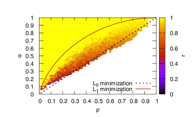
(a) $N=200$

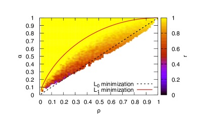
(b) $N=400$

(c) $N=800$

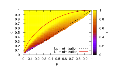
(d) $N=1600$

Figure 1: Compressed sensing phase diagram for $N=200,400,800,1600$. Each point corresponds to a single simulation. The color refers to the Pearson correlation coefficient between the true vector and the reconstructed vector. We plot the lines corresponding to the $L_{1}$ reconstruction and to the theoretical reconstruction limit, given by the $L_{0}$ condition.

The plots suggest that there exists a phase transition line $\{(\rho,\alpha^{EP}(\rho)),0\leq\rho\leq 1\}$, which is located under the $L_{1}$ line. In order to obtain the coordinates of the points along the transition line, one can proceed numerically by using a bisection-like algorithm. After discretizing the interval $0\leq\rho\leq 1$, one can select two starting values of $\alpha$ for each discretized value $\rho_{0}$. For instance, a reasonable choice, which is the one we adopt, is taking $\alpha_{0}$ on the $L_{0}$ minimization line, namely $\alpha_{0}(\rho_{0})=\rho_{0}$, and $\alpha_{1}(\rho_{0})$ on the $L_{1}$ minimization line, where $\alpha_{1}(\rho_{0})$ is expressed as [9]:

$$\alpha_{1}(\rho_{0})=2(1-\rho_{0})H(\hat{\chi}^{-1/2})+\rho_{0}.$$ (17)

In the last equation, $\hat{\chi}$ is given by the solution of [35]:

$$\hat{\chi}=\alpha^{-1}\left[2(1-\rho_{0})\left((\hat{\chi}+1)H(\hat{\chi}^{-1/2})-\hat{\chi}^{1/2}\frac{e^{-1/(2\hat{\chi})}}{\sqrt{2\pi}}\right)+\rho_{0}(\hat{\chi}+1)\right],$$ (18)

where $H(x)=\int_{x}^{+\infty}\exp(-\frac{t^{2}}{2})/(2\pi)dt$. Then, one performs the EP inference for configurations corresponding to those points and to the point $(\rho^{*},\alpha^{*})$, where $\rho^{*}=\rho_{0}$ and $\alpha^{*}=(\alpha_{0}+\alpha_{1})/2$ and computes their mean squared error. If the difference $|MSE(\alpha_{1})-MSE(\alpha^{*})|$ is negligible (i. e. smaller than a certain threshold $\delta$), then we set $\alpha_{1}=\alpha^{*}$. Otherwise, we set $\alpha_{0}=\alpha^{*}$. We recompute the middle point and repeat the procedure until we reach the desired accuracy $\Delta\alpha_{min}$ on the points located at the boundary between the successful and unsuccessful reconstruction regions. We summarize the procedure in Algorithm 2. The resulting transition line is shown in figure 2.

Algorithm 2 Bisection algorithm

procedure bisection($N,\rho_{0}$,$\alpha_{0}$,$\alpha_{1}$;$\delta$,$\Delta\alpha_{min}$)

     Set $K=\rho_{0}N$.

     Set $\alpha^{*}=(\alpha_{0}+\alpha_{1})/2$.

     repeat

         Set $M_{1}=\alpha_{1}N$.

         Generate signal $\bm{w}_{1}$ and sensing matrix $\mathbf{F}_{1}$.

         Infer $\hat{\bm{w}}_{1}$ using Algorithm 1 with inputs $\bm{y}_{1}=\mathbf{F}_{1}\bm{w}_{1}$, $\mathbf{F}_{1}$ and $\rho=\rho_{0}$.

         Compute $MSE(\alpha_{1})$ between $\hat{\bm{w}}_{1}$ and $\bm{w}_{1}$.

         Set $M^{*}=\alpha^{*}N.$

         Generate signal $\bm{w}^{*}$ and sensing matrix $\mathbf{F}^{*}$.

         Infer $\hat{\bm{w}}^{*}$ using Algorithm 1 with inputs $\bm{y}^{*}=\mathbf{F}^{*}\bm{w}^{*}$, $\mathbf{F}^{*}$ and $\rho=\rho_{0}$.

         Compute $MSE(\alpha^{*})$ between $\hat{\bm{w}}^{*}$ and $\bm{w}^{*}$.

         if $|MSE(\alpha_{1})-MSE(\alpha^{*})|>\delta$ then

              $\alpha_{0}=\alpha^{*}$.

         else

              $\alpha_{1}=\alpha^{*}$.          

         Reassign $\alpha^{*}=(\alpha_{0}+\alpha_{1})/2$.

     until $|\alpha_{1}-\alpha_{0}|/2<\Delta\alpha_{min}$

     return $\alpha^{*}$

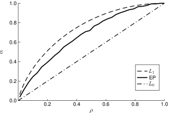
Figure 2: EP phase transition line as obtained using the bisection-like algorithm described in the main text. The number of variables is $N=1600$ and the threshold $\delta$ for the difference of the mean squared error of the evaluated points is $10^{-5}$.

We define probability of convergence as the empirical frequency that for a random instance of the signal $\bm{w}$ and of the measurement matrix $\mathbf{F}$, the algorithmic error $\epsilon_{t}$ becomes arbitrarily small after some iteration, as the maximum number of iterations $t$ is increased. In practice, we set a threshold for the error $\epsilon_{t}$ equal to $10^{-6}$ and we estimated the probability of convergence as the fraction of times the algorithm fulfilled the convergence criterion. Empirically, it turns out that the probability of convergence of EP, increases with the number of variables $N$ (not shown). Moreover, the fluctuations of the Pearson correlation coefficient $r$ and of the MSE beyond the transition line decrease as the number of variables $N$ becomes larger, whereas their average values do not seem to depend on the size of the system. We show this in the case of the MSE in figure 3, for $N=400$ and $N=1600$.

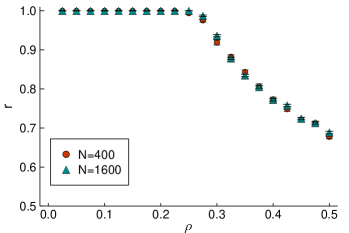
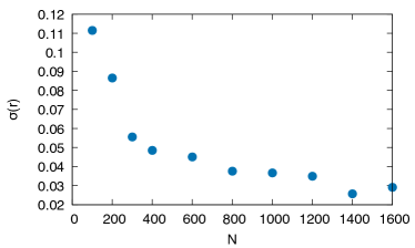
Figure 3: (a) Pearson correlation as a function of $\rho$ at $\alpha=0.5$, for $N=400$ and $N=1600$. The error bars are estimated as $\sigma(r)/N_{t}$, where $N_{t}=100$ is the number of trials. (b) Sample standard deviation of $r$ as a function of $N$. The value of the density and of the measurement rate are fixed and given by $\rho=0.4$ and $\alpha=0.55$.

Finally, we note that the mean squared error can be expressed as follows:

$$MSE=\rho MSE_{1}+(1-\rho)MSE_{2},$$ (19)

where $MSE_{1}$ is the mean squared error between the vector of the $K$ non zero components of the signal and the corresponding vector extracted from the inferred signal and $MSE_{2}$ is the mean squared error between the original and inferred vectors having the remaining $N-K$ elements as components. The latter corresponds to the squared norm of the last $N-K$ components of the inferred vector (divided by $N-K$). Beyond the CS threshold of EP, the dominant contribution to the reconstruction error comes from the estimate of the $K$ non-zero components of the reconstructed vector, implying that, overall, EP is still quite accurate in discriminating the zero entries of the signal. This is shown in figures 4 and 4, in which, respectively, $\rho MSE_{1}$ and $(1-\rho)MSE_{2}$ are compared to the total mean squared error.

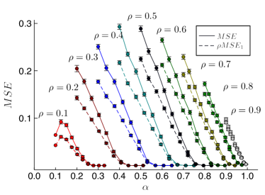
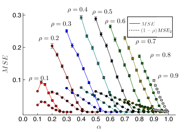
Figure 4: a) Contribution of the first $K$ components to the mean squared error (dashed lines), compared to the mean squared error itself (solid lines). (b) Contribution of the last $N-K$ components (the ‘tail’ of the vector) to the mean squared error (dotted lines), compared to the mean squared error itself (solid lines). In all plots, $N=400$, the number of simulations is 100 and each curve corresponds to a different value of $\rho$. The points are averages computed over the $N_{c}$ converged simulations and the error is estimated from the sample standard deviation $\sigma$ as $\sigma/\sqrt{N_{c}}$. From left to right, $\rho$ ranges from $0.1$ to $0.9$.

3.2 Correlated measurement matrices

We consider the case of correlated measurement matrices $\mathbf{F}$:

$$\mathbf{F}=({\bm{f}}_{1},...,{\bm{f}}_{M})^{T},$$ (20)

whose rows $\bm{f}_{i}\in\mathbb{R}^{N}$ are correlated but linearly independent samples drawn from a multivariate Gaussian distribution:

$$\bm{f}_{i}\sim\mathcal{N}(\bm{0},\mathbf{S}),\qquad i=1,...,M.$$ (21)

The covariance matrix $\mathbf{S}$ is designed according to the following functional form:

$$\mathbf{S}=\mathbf{Y}^{T}\mathbf{Y}+\bm{\Delta},$$ (22)

where $\mathbf{Y}$ is a $k\times N$ matrix with random i.i.d. Gaussian $\mathcal{N}(0,1)$ entries and having a controllable rank $k$ and $\bm{\Delta}$ is a diagonal $N\times N$ matrix with positive Gaussian i.i.d. eigenvalues. Notice that the product $\mathbf{Y}^{T}\mathbf{Y}$ is symmetric and positive semi-definite by construction. Adding the matrix $\bm{\Delta}$ ensures that $\mathbf{S}$ has maximum rank.

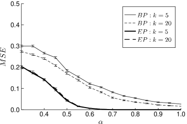
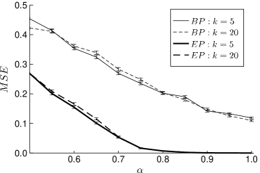
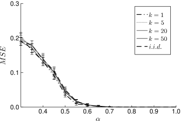
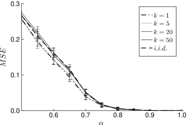
Figure 5: (a),(b) Comparison between the MSE obtained when reconstructing by means of EP and by means of EMBP in the case of correlated measurement matrices. The plot shows the MSE as evaluated over $N_{t}=1000$ converged trials and the uncertainty has been estimated as $\sigma/\sqrt{N_{t}}$, where $\sigma$ is the sample standard deviation. Regardless of the value of $\alpha$, the EMBP algorithm is not able to reconstruct correctly the signal, whereas EP achieves zero MSE beyond a critical value $\alpha_{c}(\rho)$. (c),(d) MSE resulting from the reconstruction from both i.i.d. and correlated measurement matrices. Each point was evaluated over $N_{t}=1000$ trials. Lower values of $k$ correspond to more correlated measurements. The number of variables is $N=50$ and the density of the signal is (a),(c) $\rho=0.3$ and (b),(d) $\rho=0.5$.

We first study the retrieval performance of EP and of Expectation Maximization Belief Propagation (EMBP), a similar message passing reconstruction algorithm [24, 25], implemented in MATLAB and available at http://aspics.krzakala.org.

The BP approximation lies on the independence of the entries of the sensing matrix, a condition that is not generally fulfilled in the matrices considered in this section. In particular, for small values of $k$ the covariances and the variances of $\mathbf{S}$ are of the same order of magnitude. However, as $k$ increases, these variances become dominant with respect to the off-diagonal entries of $\mathbf{S}$ and the associated multivariate Gaussian measure becomes more and more similar to the product of independent univariate Gaussian distributions. In figures 5 and 5, we compare the MSE associated with EMBP and with EP when using correlated matrices and for $\rho=0.3$, $\rho=0.5$ respectively. The signal density is learned in both cases, using Expectation Maximization in the case of EMBP and using the free energy-based variational method described in C in the case of EP. Only converged trials have been taken into account. While BP fails to correctly reconstruct the signal and to infer the signal density in the presence of the correlations we introduced in the measurements, the performance of the EP reconstruction is unaffected. As we expected, EMBP performances improve as $k$ increases. However, we note that at low enough values of $k$, such as those we have considered, EMBP never achieves zero MSE, not even when $\alpha=1$ (that is when we have as many equations as variables).

The fraction of converged trials is generally far lower in the case of EMBP than in the case of EP and decreases as $N$ is increased. For example, in the case of $k=1$, for $N=50$, it is of the order of one in a thousand of simulated trials, two orders of magnitude lower than the fraction of converged EP simulations at the same values of $N$ and $k$ (not shown).

We also plot the MSE resulting from the EP reconstruction for i.i.d. measurement matrices and correlated measurement matrices that are constructed using equations (20), (21) and (22) for various values of $k$. By considering $k=50$, $k=20$, $k=10$, $k=5$ and $k=1$, we obtain that the associated mean squared errors do not exhibit significant discrepancies, as shown in figures 5 and 5. This confirms that the EP inference of the signal is not altered with respect to the case of i.i.d. sensing matrices and retains its correct-incorrect reconstruction threshold.

Finally, we tested several algorithms for sparse reconstruction on linear systems with the same type of correlated measurement matrices considered so far. More precisely, these algorithms are Basis Pursuit [36], Orthogonal Matching Pursuit (OMP) [37], Regularized Orthogonal Matching Pursuit [38], Compressive Sampling Matching Pursuit (CoSaMP) [39], Subspace Pursuit [40], Smoothed L0 (SL0) [41], Approximate Message Passing (AMP) [13] and, again, Expectation Maximization Belief Propagation [24]. These algorithms are implemented in the C++ library KL1p [42]. This specific implementation makes use of the linear algebra library Armadillo [43, 44].

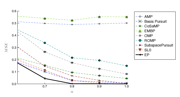
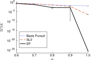
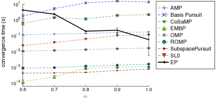
Figure 6: (a) Comparison of the MSE of various CS reconstruction algorithms in the presence of correlated measurement matrices with $k=5$. The signals to be retrieved have density $\rho=0.5$. (b) Semi-logarithmic plot of the reconstruction error of Basis Pursuit, SL0 and EP. (c) Comparison of the elapsed running time of the same reconstruction algorithms in the presence of correlated measurement matrices. In both figures, the parameters of the generated signals are given by $N=100$, $\rho=0.5$ and $\kappa$=5 and the total number of trials is $N_{t}=100$.

In order to compare the performance of these algorithms, we generated $N_{t}=100$ random gaussian i.i.d. signals of length $N=100$ and as many random correlated sensing matrices, with $k=5$. For any given pair of signal $\bm{w}$ and measurement matrix $\mathbf{F}$, we attempted to recover the original signal by means of EP and of the algorithms included in KL1p. The results are presented in figure 6. As we can see in figure 6 and as further highlighted in the semi-logarithmic plot in figure 6, EP is the only algorithm exhibiting an incorrect-correct reconstruction phase transition, whereas all the other methods that we considered fail to retrieve the signal regardless of the value of $\alpha$. In terms of running time, EP appears to be comparable to most of the other reconstruction techniques, as shown in figure 6.

4 Conclusions

We have proposed an EP-based scheme for efficient CS reconstruction whose computational complexity is dominated by a matrix inversion per iteration which requires $O(N^{3})$ operations

By analyzing the reconstruction achieved by EP in the case of undersampled linear systems with random i.i.d. measurement matrices, we showed that EP exhibits a phase transition, in analogy to other message passing inspired algorithms. We numerically computed the threshold and the related phase transition diagram and found that signal reconstruction is possible below the $L_{1}$ minimization line (see figures 1, and 2).

Finally, we investigated the case of correlated measurement matrices and found that the EP threshold persists, implying that EP is still capable of accurately retrieving the signal beyond a critical $\alpha$ and that, contrary to the case of other reconstruction algorithms, it is robust against the presence of statistical structure in the measurements.

5 Acknowledgements

We acknowledge the kind hospitality of the Physics Department of the University of Havana where part of this work has been completed. This work has received support by INFERNET – Marie Skłodowska-Curie grant agreement number 734439 – and by the SmartData@PoliTO interdepartmental center of Politecnico di Torino.

Appendix A Expectation Propagation in the zero temperature limit

In section 2, we implemented the linear constraints in equation (1) as the $\beta\rightarrow\infty$ limit of the multivariate Gaussian measure. We are going to show here how one can compute analytically this limit. Let us rewrite the previous formalism in a slightly different matrix notation. We will assume that the rank of the measurement matrix is maximum and equal to $M$, with $M<N$ (if this is not the case, we can easily remove the linearly dependent rows from the measurement matrix $\mathbf{F}$). Through Gaussian elimination, we can transform the matrix $\mathbf{F}$ to a row echelon form:

$$\mathbf{F}^{\prime}=\left[\begin{array}[]{ccc}\mathbf{I}&|&\mathbf{G}\end{array}\right]=\left[\begin{array}[]{cccccccc}1&&&&G_{1,1}&\dots&G_{1,N-M}\\ &1&&&G_{2,1}&\dots&G_{2,N-M}\\ &&\dots&&\dots&\dots&\dots\\ &&&1&G_{M,1}&\dots&G_{M,N-M}\end{array}\right]$$

The structure of the linear constraint induced by the row echelon representation suggests to split the $\bm{w}$ variable into two sets of variables: the first $M$ variables (dependent) and a second set of $N-M$ variables (independent). To do so, we define:

$${\bm{w}}=:({\bm{w}}^{(d)},\bm{w}^{(i)})=w_{1}^{(d)},\dots,w_{M}^{(d)},w_{1}^{(i)},\dots,w_{N-M}^{(i)}$$

where ${\bm{w}}^{(d)}\in\mathbb{R}^{M}$, and ${\bm{w}}^{(i)}\in\mathbb{R}^{N-M}$. The linear constraint in equation (1) now reads:

$${\bm{w}}^{(d)}+\mathbf{G}{\bm{w}}^{(i)}={\bm{y}}^{\prime}$$

where ${\bm{y}}^{\prime}\in\mathbb{R}^{M}$ is the transformed measurement vector. Assuming, as in the previous subsection, a Gaussian prior for the $\bm{w}^{(i)}$ variables, there follows a Gaussian statistics on the ${\bm{w}}^{(d)}$ variables with consistent moments:

$${\bm{\bar{}}{\bm{w}}}^{(d)}=-\mathbf{G}\bar{{\bm{w}}}^{(i)}+{\bm{y}^{\prime}}$$

$$\bm{\Sigma}_{{\bm{w}}^{(i)}}=\left(\mathbf{D}_{{\bm{w}}^{(i)}}+\mathbf{G}^{T}\mathbf{D}_{{\bm{w}}^{(d)}}\mathbf{G}\right)^{-1},\quad\bm{\Sigma}_{{\bm{w}}^{(d)}}=\mathbf{G}\bm{\Sigma}_{{\bm{w}}^{(i)}}\mathbf{G}^{T}$$

where the $\bm{D}_{{\bm{w}}^{(d)}},\bm{D}_{{\bm{w}}^{(i)}}$ are the diagonal matrices whose entries are the inverses of the variances of the Gaussian priors associated with the dependent and independent variables, respectively. We note that from the previous relations the moments of the dependent ${\bm{w}}^{(d)}$ variables can be directly related to those of the ${\bm{w}}^{(i)}$ variables, which allows us to compute everything in terms of the inverse of a smaller matrix of size $\left(N-M\right)\times(N-M)$ compared to the finite temperature case.

At this point, the parameters $\bm{a}$ and $\bm{d}$ can be updated by moment matching as described in section 2.

Appendix B Moments of the spike-and-slab prior

We use the spike-and-slab prior, defined as:

$$\psi(w_{n})=(1-\rho)\delta(w_{n})+\frac{\rho}{\sqrt{2\pi\lambda}}e^{-\frac{w_{n}^{2}}{2\lambda}},$$ (23)

where $\rho=K/N$ is the density of the signal $\bm{w}$. For spike-and-slab priors, the $n$-th marginal of the tilted distribution (9) is given by:

$$Q^{(n)}(w_{n})=\frac{1}{Z_{Q^{(n)}}}\tilde{Q}_{n}(w_{n})\psi_{n}(w_{n})$$ (24)

in which:

$$\tilde{Q}_{n}(w_{n})=\frac{1}{\sqrt{2\pi\Sigma^{\prime}_{n}}}e^{-\frac{(w_{n}-\bar{w}^{\prime}_{n})^{2}}{2\Sigma^{\prime}_{n}}},$$ (25)

where we have denoted $\left(\bar{w}_{(n)}\right)_{n}$ and $\left(\Sigma_{(n)}\right)_{n,n}$ by $\bar{w}^{\prime}_{n}$ and $\Sigma^{\prime}_{n}$, respectively, in order to simplify the notation.

The partition function in (24) reads:

$$Z_{Q^{(n)}}=(1-\rho)\frac{1}{\sqrt{2\pi\Sigma^{\prime}_{n}}}e^{-\frac{\bar{w}_{n}^{{}^{\prime}2}}{2\Sigma^{\prime}_{n}}}+\frac{\rho}{\sqrt{2\pi(\lambda+\Sigma^{\prime}_{n})}}e^{-\frac{1}{2}\frac{\bar{w}_{n}^{{}^{\prime}2}}{\lambda+\Sigma^{\prime}_{n}}},$$ (26)

and the first and second moment of $w_{n}$ with respect to $Q^{(n)}$ are given by:

$$\langle w_{n}\rangle_{Q^{(n)}}=\frac{1}{Z_{Q^{(n)}}}\frac{\rho}{\sqrt{2\pi(\lambda+\Sigma^{\prime}_{(n)})}}\frac{\lambda\bar{w}^{\prime}_{n}}{\lambda+\Sigma^{\prime}_{n}}e^{-\frac{1}{2}\frac{\bar{w}_{n}^{{}^{\prime}2}}{\lambda+\Sigma^{\prime}_{n}}},$$ (27)

and by:

$$\langle w_{n}^{2}\rangle_{Q^{(n)}}=\frac{1}{Z_{Q^{(n)}}}\frac{\rho}{\sqrt{2\pi(\lambda+\Sigma^{\prime}_{n})}}\left(\frac{\lambda\Sigma^{\prime}_{n}(\lambda+\Sigma^{\prime}_{n})+\lambda^{2}\bar{w}_{n}^{{}^{\prime}2}}{(\lambda+\Sigma^{\prime}_{n})^{2}}\right)e^{-\frac{1}{2}\frac{\bar{w}_{n}^{{}^{\prime}2}}{\lambda+\Sigma^{\prime}_{n}}},\quad$$ (28)

respectively.

Appendix C Learning of the density parameter of the prior

C.1 The EP Free Energy function

Let us consider equation (9) and rewrite it through equation (6) as:

$$Q^{(n)}({\bm{w}}|\mathbf{F},{\bm{y}}) := \frac{1}{Z_{Q^{(n)}}}e^{-\beta\frac{\left({\bm{y}}-\mathbf{F}\bm{w}\right)^{T}\cdot\left({\bm{y}}-\mathbf{F}\bm{w}\right)}{2}}\psi_{n}(w_{n})\prod_{l\neq n}\phi_{l}(w_{l};a_{l,}d_{l})$$ (29)

$$= \frac{Z_{Q}}{Z_{{Q}^{(n)}}}Q({\bm{w}}|\mathbf{F},{\bm{y}})\frac{\psi_{n}(w_{n})}{\phi_{n}(w_{n})}\,.$$

We define:

$$Z_{EP}=Z_{Q}\prod_{n=1}^{N}\frac{Z_{Q^{(n)}}}{Z_{Q}}=\frac{\prod_{n=1}^{N}Z_{Q^{(n)}}}{Z^{N-1}_{Q}},$$ (30)

from which the so-called EP free energy follows:

$$F_{EP}=(N-1)\log Z_{Q}-\sum_{n=1}^{N}\log Z_{Q^{(n)}}.$$ (31)

The converged means $\bm{a}$ and variances $\bm{d}$ of EP, which fulfill the moment matching conditions (11) for all $n=1,\dots,N$, are fixed points of the EP free energy, where the latter are obtained from:

$$0 = \frac{\partial F_{EP}}{\partial a_{n}}=(N-1)\langle w_{n}\rangle_{Q}-\sum_{l\neq n}\langle w_{n}\rangle_{Q^{(l)}},$$ (32)

$$0 = \frac{\partial F_{EP}}{\partial d_{n}}=(N-1)\langle w_{n}^{2}\rangle_{Q}-\sum_{l\neq n}\langle w_{n}^{2}\rangle_{Q^{(l)}},$$ (33)

for $n=1,\dots,N$. In order to show this, we shall prove that the moment matching conditions imply that (32) and (33) are satisfied. We have for $\langle w_{n}\rangle_{Q^{(l)}}$ and $\langle w_{n}^{2}\rangle_{Q^{(l)}}$:

$$\langle w_{n}^{\alpha}\rangle_{Q^{(l)}} = \int\frac{Z_{Q}}{Z_{Q^{(l)}}}Q(\bm{w})\frac{\psi_{l}(w_{l})}{\phi_{l}(w_{l})}w_{n}^{\alpha}d\bm{w}=\int Q(\bm{w})\frac{Q^{(l)}(w_{l})}{Q(w_{l})}w_{n}^{\alpha}d\bm{w}=$$

$$= \left\langle\int_{-\infty}^{+\infty}\frac{Q(w_{n},w_{l})}{Q(w_{l})}w_{n}^{\alpha}dw_{n}\right\rangle_{Q^{(l)}(w_{l})},\quad\alpha=1,2$$

In the last equality, for $\alpha=1$ ($\alpha=2$), the integral being averaged w.r.t. ${Q^{(l)}(w_{l})}$ is the first (second) moment of $w_{n}$, conditioned on $w_{l}$ and computed w.r.t. $Q$. These moments depend on $w_{l}$ through the mean (squared mean) of $Q(w_{n}|w_{l})$. As such mean depends linearly on $w_{l}$, $\langle w_{n}\rangle_{Q(w_{n}|w_{l})}$ and $\langle w^{2}_{n}\rangle_{Q(w_{n}|w_{l})}$ depend on $w_{l}$ linearly and quadratically, respectively. Therefore, for $\alpha=1,2$, by the moment matching conditions, we have that:

$$\left\langle\int_{-\infty}^{+\infty}\frac{Q(w_{n},w_{l})}{Q(w_{l})}w_{n}^{\alpha}dw_{n}\right\rangle_{Q^{(l)}(w_{l})}=\left\langle\int_{-\infty}^{+\infty}\frac{Q(w_{n},w_{l})}{Q(w_{l})}w_{n}^{\alpha}dw_{n}\right\rangle_{Q(w_{l})},$$ (34)

implying that $\langle w_{n}^{\alpha}\rangle_{Q^{(l)}}=\langle w_{n}^{\alpha}\rangle_{Q}$ and thus that the conditions (32) and (33) are identically fulfilled.

C.2 Learning of the density

We are interested in finding the maximum likelihood value of the density parameter $\rho$ which appears in the prior factors $\psi_{n}(w_{n})$. The likelihood of the parameters of the prior is given by:

$$P(\bm{y}|\rho,\lambda) = \int d\bm{w}P(\bm{y},\bm{w}|\rho,\lambda)=$$ (35)

$$= \int d\bm{w}P(\bm{y}|\bm{w})P(\bm{w}|\rho,\lambda)=Z(\rho,\lambda)$$ (36)

and maximizing this likelihood corresponds to minimizing the associated free energy $F(\rho,\lambda)=-\log Z(\rho,\lambda)$.

At the fixed point of EP, the free energy is approximated by $F_{EP}$ and the parameters can be learned by gradient descent. In particular, we have for the signal density $\rho$:

$$\rho^{(t+1)}\leftarrow\rho^{(t)}-\eta\frac{\partial F_{EP}}{\partial\rho},$$ (37)

where $t$ denotes the current iteration and $\eta$ is a learning rate. In the simulations of this paper, we have taken $\eta=5\times 10^{-4}$.

The parameters of the prior enter in the EP free energy through the contributions associated with each of the tilted distributions. Such contributions read:

$$F_{Q^{(n)}}=-\log Z_{Q^{(n)}}=-\log\left(\int\tilde{Q}^{(n)}(\bm{w}|\bm{y})\psi_{n}(w_{n})d\bm{w}\right)$$ (38)

for

$$\tilde{Q}^{(n)}(\bm{w}|\bm{y})=e^{-\frac{1}{2}({\bm{w}}-\bar{{\bm{w}}}_{(n)})^{T}\Sigma_{(n)}^{-1}({\bm{w}}-\bar{{\bm{w}}}_{(n)})}.$$ (39)

Therefore, we have for $\frac{\partial F_{EP}}{\partial\rho}$:

$$\frac{\partial F_{EP}}{\partial\rho}=\sum_{n=1}^{N}\frac{\partial F_{Q^{(n)}}}{\partial\rho},$$ (40)

where:

$$\frac{\partial F_{Q^{(n)}}}{\partial\rho}=-\frac{1}{Z_{Q^{(n)}}}\int\tilde{Q}_{n}(w_{n})\frac{\partial\psi_{n}}{\partial\rho}(w_{n})dw_{n},$$ (41)

and:

$$\frac{\partial\psi_{n}}{\partial\rho}(w_{n})=-\delta(w_{n})+\frac{1}{\sqrt{2\pi\lambda}}e^{-\frac{w_{n}^{2}}{2\lambda}},$$ (42)

yielding:

$$\frac{\partial F_{EP}}{\partial\rho}=\sum_{n=1}^{N}\frac{\frac{1}{\sqrt{2\pi\Sigma_{n,n}}}e^{-\frac{\bar{w}_{n}^{2}}{2\Sigma_{n,n}}}-\frac{1}{\sqrt{2\pi(\lambda+\Sigma_{n,n})}}e^{-\frac{1}{2}\frac{\bar{w}_{n}^{2}}{\lambda+\Sigma_{n,n}}}}{(1-\rho)\frac{1}{\sqrt{2\pi\Sigma_{n,n}}}e^{-\frac{\bar{w}_{n}^{2}}{2\Sigma_{n,n}}}+\frac{\rho}{\sqrt{2\pi(\lambda+\Sigma_{n,n})}}e^{-\frac{1}{2}\frac{\bar{w}_{n}^{2}}{\lambda+\Sigma_{n,n}}}}.$$ (43)

By taking the derivative w.r.t. $\rho$ one more time, we see that $F_{EP}$ is a strictly convex function of $\rho$ for $\lambda>0$:

$$\frac{\partial^{2}F_{EP}}{\partial\rho^{2}}=\sum_{n=1}^{N}\left[\frac{\frac{1}{\sqrt{2\pi\Sigma_{n,n}}}e^{-\frac{\bar{w}_{n}^{2}}{2\Sigma_{n,n}}}-\frac{1}{\sqrt{2\pi(\lambda+\Sigma_{n,n})}}e^{-\frac{1}{2}\frac{\bar{w}_{n}^{2}}{\lambda+\Sigma_{n,n}}}}{(1-\rho)\frac{1}{\sqrt{2\pi\Sigma_{n,n}}}e^{-\frac{\bar{w}_{n}^{2}}{2\Sigma_{n,n}}}+\frac{\rho}{\sqrt{2\pi(\lambda+\Sigma_{n,n})}}e^{-\frac{1}{2}\frac{\bar{w}_{n}^{2}}{\lambda+\Sigma_{n,n}}}}\right]^{2},$$ (44)

which guarantees that the sought value of $\rho$ is unique at fixed $\bar{w}_{n}$ and $\Sigma_{n,n}$.

References

- Candès and Romberg [2005a] E. J. Candès and J. K. Romberg. Signal recovery from random projections. In Computational Imaging III, volume 5674, pages 76–87. International Society for Optics and Photonics, 2005a.
- Donoho [2006] D. L. Donoho. Compressed sensing. IEEE Transactions on information theory, 52(4):1289–1306, 2006.
- Candès and Wakin [2008] E. J. Candès and M. B. Wakin. An introduction to compressive sampling [a sensing/sampling paradigm that goes against the common knowledge in data acquisition]. IEEE signal processing magazine, 25(2):21–30, 2008.
- Zhang et al. [2015] Z. Zhang, Y. Xu, J. Yang, X. Li, and D. Zhang. A survey of sparse representation: algorithms and applications. IEEE access, 3:490–530, 2015.
- Mishali et al. [2011] M. Mishali, Y. C. Eldar, O. Dounaevsky, and E. Shoshan. Xampling: Analog to digital at sub-nyquist rates. IET circuits, devices & systems, 5(1):8–20, 2011.
- Mézard et al. [2002] M. Mézard, G. Parisi, and R. Zecchina. Analytic and algorithmic solution of random satisfiability problems. Science, 297(5582):812–815, 2002.
- Mulet et al. [2002] R. Mulet, A. Pagnani, M. Weigt, and R. Zecchina. Coloring random graphs. Physical review letters, 89(26):268701, 2002.
- Mezard and Montanari [2009] M. Mezard and A. Montanari. Information, physics, and computation. Oxford University Press, 2009.
- Kabashima et al. [2009] Y. Kabashima, T. Wadayama, and T. Tanaka. A typical reconstruction limit for compressed sensing based on -norm minimization. Journal of Statistical Mechanics: Theory and Experiment, 2009(09):L09003, 2009.
- Mézard et al. [1987] M. Mézard, G. Parisi, and M. Virasoro. Spin glass theory and beyond: An Introduction to the Replica Method and Its Applications, volume 9. World Scientific Publishing Company, 1987.
- Candès and Tao [2006a] E. J. Candès and T. Tao. Near-optimal signal recovery from random projections: Universal encoding strategies? IEEE Transactions on Information Theory, 52(12):5406–5425, 2006a.
- Candès [2008] E. J. Candès. The restricted isometry property and its implications for compressed sensing. Comptes Rendus Mathematique, 346(9):589 – 592, 2008.
- Donoho et al. [2009] D. L. Donoho, A. Maleki, and A. Montanari. Message-passing algorithms for compressed sensing. Proceedings of the National Academy of Sciences, 106(45):18914–18919, 2009.
- Nguyen and Shin [2013] T. L. N. Nguyen and Y. Shin. Deterministic sensing matrices in compressive sensing: A survey. The Scientific World Journal, 2013, 2013.
- Applebaum et al. [2009] L. Applebaum, S. D. Howard, S. Searle, and R. Calderbank. Chirp sensing codes: Deterministic compressed sensing measurements for fast recovery. Applied and Computational Harmonic Analysis, 26(2):283 – 290, 2009.
- Ni et al. [2009] K. Ni, P. Mahanti, S. Datta, S. Roudenko, and D. Cochran. Image reconstruction by deterministic compressed sensing with chirp matrices. volume 7497, 2009.
- Howard et al. [2008] S. D. Howard, A. R. Calderbank, and S. J. Searle. A fast reconstruction algorithm for deterministic compressive sensing using second order Reed-Muller codes. In 2008 42nd Annual Conference on Information Sciences and Systems, pages 11–15, 2008.
- Candès and Tao [2006b] E. J. Candès and T. Tao. Near-optimal signal recovery from random projections: Universal encoding strategies? IEEE Transactions on Information Theory, 52(12):5406–5425, 2006b.
- Candès et al. [2006] E. J. Candès, J. Romberg, and T. Tao. Robust uncertainty principles: exact signal reconstruction from highly incomplete frequency information. IEEE Transactions on Information Theory, 52(2):489–509, 2006.
- Margosian et al. [2007] P. Margosian, G. DeMeester, and H. Liu. Partial Fourier Acquisition in MRI. 2007.
- Ravazzi et al. [2017] C. Ravazzi, G. Coluccia, and E. Magli. Image reconstruction from partial Fourier measurements via curl constrained sparse gradient estimation. In 2017 IEEE International Conference on Acoustics, Speech and Signal Processing (ICASSP), pages 4745–4749, 2017.
- Anitori et al. [2013] L. Anitori, A. Maleki, M. Otten, R. G. Baraniuk, and P. Hoogeboom. Design and analysis of compressed sensing radar detectors. IEEE Transactions on Signal Processing, 61:813–827, 2013.
- Holger [2009] R. Holger. Circulant and Toeplitz matrices in compressed sensing. CoRR, abs/0902.4394, 2009.
- Krzakala et al. [2012a] F. Krzakala, M. Mézard, F. Sausset, Y. F. Sun, and L. Zdeborová. Statistical-physics-based reconstruction in compressed sensing. Phys. Rev. X, 2:021005, 2012a.
- Krzakala et al. [2012b] F. Krzakala, M. Mézard, F. Sausset, Y. Sun, and L. Zdeborová. Probabilistic reconstruction in compressed sensing: algorithms, phase diagrams, and threshold achieving matrices. Journal of Statistical Mechanics: Theory and Experiment, 2012(08):P08009, 2012b.
- Mitchell and Beauchamp [1988] T. J. Mitchell and J. J. Beauchamp. Bayesian variable selection in linear regression. Journal of the American Statistical Association, 83(404):1023–1032, 1988.
- Opper and Winther [2000] M. Opper and O. Winther. Gaussian processes for classification: mean-field algorithms. Neural Computation, 12(11):2655–2684, 2000.
- Opper and Winther [2001] M. Opper and O. Winther. Adaptive and self-averaging Thouless-Anderson-Palmer mean-field theory for probabilistic modeling. Physical Review E, 64(5):056131, 2001.
- Minka [2001] T. P. Minka. Expectation propagation for approximate Bayesian inference. In Proceedings of the Seventeenth conference on Uncertainty in artificial intelligence, pages 362–369. Morgan Kaufmann Publishers Inc., 2001.
- Braunstein et al. [2017] A. Braunstein, A. P. Muntoni, and A. Pagnani. An analytic approximation of the feasible space of metabolic networks. Nature communications, 8:14915, 2017.
- Muntoni et al. [2018] A. P. Muntoni, R. D. H. Rojas, A. Braunstein, A. Pagnani, and I. P. Castillo. Non-convex image reconstruction via expectation propagation. arXiv preprint arXiv:1809.03958, 2018.
- Seeger [2008] Matthias W. Seeger. Bayesian inference and optimal design for the sparse linear model. The Journal of Machine Learning Research, 9:759–813, 2008.
- Hernández-Lobato et al. [2015] J. M. Hernández-Lobato, D. Hernández-Lobato, and A. Suárez. Expectation propagation in linear regression models with spike-and-slab priors. Machine Learning, 99(3):437–487, 2015.
- Braunstein et al. [2019] A. Braunstein, G. Catania, and L. Dall’Asta. Loop corrections in spin models through density consistency. Phys. Rev. Lett., 123:020604, 2019.
- Kabashima et al. [2012] Y. Kabashima, T. Wadayama, and T. Tanaka. Erratum: A typical reconstruction limit of compressed sensing based on -norm minimization. Journal of Statistical Mechanics: Theory and Experiment, 2012(07):E07001, 2012.
- Candès and Romberg [2005b] E. J. Candès and J. Romberg. -magic: Recovery of sparse signals via convex programming. URL: www.acm.caltech.edu/l1magic/downloads/l1magic.pdf, 4:14, 2005b.
- Tropp and Gilbert [2007] J. A. Tropp and A. C. Gilbert. Signal recovery from random measurements via orthogonal matching pursuit. IEEE Transactions on Information Theory, 53(12):4655–4666, 2007.
- Needell and Vershynin [2010] D. Needell and R. Vershynin. Signal recovery from incomplete and inaccurate measurements via regularized orthogonal matching pursuit. IEEE Journal of Selected Topics in Signal Processing, 4(2):310–316, 2010.
- Needell and Tropp [2009] D. Needell and J. A. Tropp. CoSaMP: Iterative signal recovery from incomplete and inaccurate samples. Applied and Computational Harmonic Analysis, 26(3):301 – 321, 2009.
- Dai and Milenkovic [2009] W. Dai and O. Milenkovic. Subspace pursuit for compressive sensing signal reconstruction. IEEE Transactions on Information Theory, 55(5):2230–2249, 2009.
- Mohimani et al. [2009] H. Mohimani, M. Babaie-Zadeh, and C. Jutten. A fast approach for overcomplete sparse decomposition based on smoothed norm. IEEE Transactions on Signal Processing, 57(1):289–301, 2009.
- Gebel [2012] R. Gebel. KL1p – A portable C++ library for Compressed Sensing, 2012.
- Sanderson and Curtin [2018] C. Sanderson and R. Curtin. A User-Friendly Hybrid Sparse Matrix Class in C++. Lecture Notes in Computer Science (LNCS), 10931:422–430, 2018.
- Sanderson and Curtin [2016] C. Sanderson and R. Curtin. Armadillo: a template-based C++ library for linear algebra. Journal of Open Source Software, 1:26, 2016.