Absorbing Random Walks Interpolating Between Centrality Measures on Complex Networks

Abstract

Centrality, which quantifies the “importance” of individual nodes, is among the most essential concepts in modern network theory. As there are many ways in which a node can be important, many different centrality measures are in use. Here, we concentrate on versions of the common betweenness and closeness centralities. The former measures the fraction of paths between pairs of nodes that go through a given node, while the latter measures an average “inverse distance” between a particular node and all other nodes. Both centralities only consider shortest paths (i.e., geodesics) between pairs of nodes. Here we develop a method, based on absorbing Markov chains, that enables us to continuously interpolate both of these centrality measures away from the geodesic limit and toward a limit where no restriction is placed on the length of the paths the walkers can explore. At this second limit, the interpolated betweenness and closeness centralities reduce, respectively, to the well-known current betweenness and resistance closeness (information) centralities. The method is tested numerically on four real networks, revealing complex changes in node centrality rankings with respect to the value of the interpolation parameter. Non-monotonic betweenness behaviors are found to characterize nodes that lie close to inter-community boundaries in the studied networks.

I Introduction

Modern network theory has evolved through a synthesis of mathematical graph theory Euler (1736, 1956); Bollobás (1998) with problems and methods from social sciences Moreno (1934); Opsahl et al. (2010) and physics Kirchhoff (1847); O’Toole (1958); Albert and Barabási (2002); Caldarelli (2007); Dorogovtsev et al. (2008); Newman (2010); Estrada (2011), into a powerful paradigm for analysis of complex systems consisting of interacting entities. Current interdisciplinary applications include modeling of transport in porous media and composites Blunt et al. (2013); Savani et al. (2017), reaction networks in chemical synthesis Shamboek et al. (2019), food webs in ecology Rossberg (2013), transportation and distribution networks Verma et al. (2014); Xu et al. (2014); Gurfinkel et al. (2015), economics and sociology Kutner et al. (2019), the Internet and the World Wide Web Tiropanis et al. (2015), and many more.

The focus of the present paper is centrality, which, together with the adjacency relationship and the degree distribution, is one of the most basic and widely studied concepts in network theory. Centrality measures are prescriptions for quantitatively assigning importance to nodes in complex networks, and the power of the concept stems from the flexibility of characterizing importance in different ways. Applications of centrality measures are widespread, ranging from Internet searches (Google’s PageRank algorithm Page et al. (1999)) to determinations of proteins necessary for cell survival Jeong et al. (2001).

In fact, centrality results are not just useful to identify important nodes: with specific, quantitative information about individual nodes, a centrality that reproduces this information can reveal principles inherent in the structure of the network. Along these lines, in Xu et al. (2014) we investigated the architecture of the Florida electric power grid. In particular, we found a strong correlation between the known generating capacities of power plants and the values of a centrality based on Estrada’s communicability concept Estrada and Hatano (2008); Estrada et al. (2009). This centrality has a parameter that controls the (graph) distance over which nodes can influence each other. Quantification of such correlations between node attributes and network structure requires centrality measures with a built-in tuning parameter.

Here we develop an interpolation scheme connecting members of a set of four common centrality measures. Two of these measure how “close” a node is to others (closeness), while the other two measure a node’s tendency to lie on paths connecting pairs of other nodes (betweenness). Our main result is a new parametrization, based on absorbing random walks and their correspondence to electrical resistor networks Doyle and Snell (1984); Newman (2005); Brandes and Fleischer (2005); Klein and Randić (1993), that interpolates between the two betweenness measures and between the two closeness measures, respectively. In contrast to the parameter in the communicability centrality, our random-walk parameter tunes the centralities’ preference for shortest paths (geodesics) versus longer paths. Using this parameter, harmonic closeness centrality Dekker (2005); Rochat (2009); Newman (2010) (based on geodesics, as described below) is deformed into a closeness centrality based on the Klein resistance distance Brandes and Fleischer (2005); Klein and Randić (1993). Furthermore, using exactly the same parametrized absorbing random walk, the geodesic betweenness centrality Anthonisse (1971); Freeman (1977) is deformed into Newman’s random-walk betweenness Newman (2005). These four measures thus represent a natural class: walker-flow centralities. Equations defining the four limiting centralities we consider are given in Sec. II.2.

As noted below, our work is not the first concerning interpolations between different centrality measures. However, to the best of our knowledge, it is the first to interpolate between the four walker-flow centralities both (a) precisely and (b) using the same parameter for both the closeness and betweenness continua. Furthermore, our interpolation is based on an easy-to-visualize random walk, allowing analysis at both the microscopic (individual walker step) and macroscopic (final centrality weighting) levels. Also, the transition probabilities of the random walk are closely related to the physics of lossy power transmission lines, allowing connections to the engineering literature, e.g., Steer (2010).

We perform numerical tests of our analytical interpolation formalism on four real example networks of moderate size: a network of social interactions in a group of kangaroos kan (2017); Grant (1973), Zachary’s well-known karate club network Zachary (1977), and two versions of the electrical power grid of the U.S. state of Florida Dale et al. (2009). Two of these networks are weighted and two are unweighted, and they range from strongly connected to relatively sparse. The numerical centrality rankings of the nodes are found to vary, not just between the closeness and betweenness measures, but also with the value of the interpolation parameter. The dependence of the individual centrality values on the interpolation parameter is generally smooth, but not necessarily monotonic. Plateaus and extrema in the intermediate parameter range reveal the existence of nearly degenerate paths and the proximity of certain nodes to community boundaries in the network.

In recent work, Bozzo and Franceschet Bozzo and Franceschet (2013), and Tizghadam and Leon-Garcia Tizghadam and Leon-Garcia (2010), have found that random-walk betweenness can be written in terms of resistance distances and the closely related pseudo-inverse of the graph Laplacian. Alamgir and von Luxburg Alamgir and Luxburg (2011) present an interpolation between graph distance and resistance distance, which is equivalent to an interpolation (different from ours) between closeness and resistance closeness. Avrachenkov et al. Avrachenkov et al. (2013, 2015) present two betweenness-like measures, where a parameter tunes the centrality’s preference for geodesics. However, these do not precisely reduce to the betweenness. Kivimäki et al. Kivimäki et al. (2016, 2014) introduce the randomized-shortest-path (RSP) framework, which assigns Boltzmann weights to all paths in the network. Their inverse temperature parameter also tunes the preference for geodesics. In Kivimäki et al. (2016), RSP is used to interpolate between graph distance and resistance distance, while in Kivimäki et al. (2014) it is used to interpolate between random-walk betweenness and a measure similar to standard betweenness centrality. In Bavaud and Guex (2012), Bavaud and Guex accomplish a weighting equivalent to RSP through the minimization of a free-energy functional. Françoisse et al. also reach similar results with a different path-weighting scheme in Françoisse et al. (2017). Estrada, Higham, and Hatano Estrada et al. (2009) calculate a version of betweenness centrality by assigning lower weights to longer paths.

The remainder of this paper is organized as follows. In Sec. II.1, we introduce notations and conventions. In Sec. II.2, we discuss well-known centrality measures. In Sec. II.3, we develop two new parametrized centralities, based on a specific absorbing random walk, that interpolate between (a) closeness and resistance-closeness centralities and (b) betweenness and random-walk betweenness centralities. In Sec. III.1, we report the behavior of these centralities on four example networks. In Sec. III.2, we use the numerical examples to explain how the presence of similarly-long paths leads to specific centrality behaviors. In Sec. III.3, we provide a model for the non-monotonicity encountered in some of the numerics. In Sec. IV, we provide concluding comments and discuss plans for future study. Some technical details are addressed in four appendices.

II Walker-Flow Centralities

II.1 Notation and conventions

The most commonly studied centrality measures can be found in, e.g., Ch.7 of Newman (2010), and many can be written in the matrix form:

$$c_{i}=\sum_{j}\mathbf{M}_{ij},$$ (1)

where $c_{i}$ is the centrality of node $i$. The matrix element $\mathbf{M}_{ij}$ encodes the level of influence that node $j$ exerts on node $i$, and the final centrality is the sum of such influences. Commonly, centrality measures include a normalization factor to ensure that $\sum_{i}c_{i}=1$. In this paper, to better facilitate the inter-centrality comparisons in Sec. III, we will only deal with unnormalized centrality measures.

We concentrate on weighted, undirected networks, so that the adjacency matrix $\mathbf{A}$ is symmetric with, the weights of its nonzero elements denoting affinities between nodes. In other words: as $\mathbf{A}_{ij}$ increases, nodes $i$ and $j$ become more closely associated Kivimäki et al. (2014). Setting $\mathbf{M}=\mathbf{A}$ results in the weighted degree centrality: $c_{i}=A_{i}$, where $A_{i}=\sum_{j}\mathbf{A}_{ij}$ is the weighted degree of node $i$. (Unweighted networks will be treated as special cases of weighted networks, in which all nonzero $\mathbf{A}_{ij}=1$.)

Many commonly studied centralities make use of the graph distance between nodes. The weighted graph distance, $d_{ij}$, is the length of the shortest edge path from node $i$ to $j$, where the length of a given edge $(a,b)$ is $d_{(a,b)}=(\mathbf{A}_{ab})^{-1}$. Defining edge lengths to be inverses of the nonzero weighted adjacency-matrix elements is standard practice when using affinity weights in the adjacency matrix: distance is considered to be the inverse of affinity Newman (2001); Kivimäki et al. (2014); Opsahl et al. (2010). Note that $d_{ab}$ need not equal $d_{(a,b)}$, since the shortest weighted path from $a$ to $b$ does not necessarily follow the edge $(a,b)$.

II.2 Centralities based on shortest paths, resistor networks, and random walks

II.2.1 Closeness

A prominent centrality based on graph distances is Bavelas’s original closeness centrality $c^{\mathrm{CLO}}_{i}=(\sum_{j}d_{ij})^{-1}$ Bavelas (1950), here modified for weighted graphs as in Opsahl et al. (2010). This closeness measure cannot be put into the form of Eq. (1), but in Newman (2010) Newman argues for the superiority of a modified closeness:

$$\mathbf{M}^{\mathrm{HCL}}_{ij}=d_{ij}^{-1}.$$ (2)

This measure is referred to as the harmonic closeness centrality (HCL) and is studied in Latora and Marchiori (2001); Rochat (2009); Dekker (2005). The present paper deals primarily with the harmonic closeness and measures that can be similarly described in the form of Eq. (1). Unless otherwise specified, any mention of “closeness” will refer to the harmonic type. However, the ideas presented here can be straightforwardly applied to the standard closeness as well. This is because we develop generalizations of the $d_{ij}$ themselves, so either form, $(\sum_{j}d_{ij})^{-1}$ or $\sum_{j}d_{ij}^{-1}$, can be calculated.

In Brandes and Fleischer (2005), Brandes and Fleischer define a version of closeness centrality where the graph distance $d_{ij}$ is replaced by Klein and Randić’s resistance distance $R^{\mathrm{eff}}_{ij}$ Klein and Randić (1993). They prove the resulting centrality measure equivalent to the information centrality Stephenson and Zelen (1989), whose original definition made no reference to resistor networks. This centrality is given by $c^{\mathrm{INF}}_{i}=1/\sum_{j}R^{\mathrm{eff}}_{ij}=1/\sum_{j}I^{-1}_{ij}$. Here, $I_{ij}$ is the current flowing from $i$ to $j$ when a unit potential difference is introduced between those nodes. (The last equality is true by the definition of resistance distance; $R^{\mathrm{eff}}_{ij}$ is just the inverse of the current flow from $i$ to $j$.)

Alternatively, starting from the harmonic closeness centrality (HCL), rather than the original closeness, enables us to work with the centrality matrix $\mathbf{M}$. Following the same substitutions as in Brandes and Fleischer (2005), we obtain

$$\mathbf{M}^{\mathrm{RCC}}_{ij}=\frac{1}{R^{\mathrm{eff}}_{ij}}=I_{ij}.$$ (3)

Due to the similarity with HCL, the centrality of Eq. (3) can be termed the resistance-closeness centrality (RCC) (or harmonic information centrality). Eqs. (2-3) have the same structure; the difference is that HCL only considers geodesics (as captured by the weighted graph distance $d$), while RCC considers currents (encoded by $R^{\mathrm{eff}}$) that explore the entire network. In Sec. II.3, we derive a parameter that can interpolate between these two limits. This derivation relies on a useful isomorphism between random walks on networks and currents in corresponding resistor networks. Reference Doyle and Snell (1984) describes this isomorphism and provides an equation for $R^{\mathrm{eff}}$ in terms of random walks.

II.2.2 Betweenness

One of the most common centrality measures, betweenness Newman (2010); Anthonisse (1971); Freeman (1977), is defined as

$$\mathbf{M}^{\mathrm{BET}}_{ij}=\sum_{s}n_{sij}/g_{sj}.$$ (4)

Here, $g_{sj}$ counts the number of shortest paths between node $s$ and node $j$, while $n_{sij}$ counts the number of such paths that pass through $i$.

As an example of the random-walk/resistor-network isomorphism, in Newman (2005), Newman re-frames his random-walk centrality in terms of electrical currents $I$ flowing along network edges, each of which has an equal resistance. This current-betweenness centrality (CBT) can be written similarly to the standard betweenness of Eq. (4) as

$$\mathbf{M}^{\mathrm{CBT}}_{ij}=\sum_{s}I_{sij}/I_{sj}.$$ (5)

Here, $I_{sij}$ denotes the current passing through node $i$ when a current $I_{sj}$ is passed into the network at $s$ and flows out of the network at $j$. The notation here is chosen to reveal the similarity to Eq. (4). (It is necessary to separately denote the current flowing on an edge from $i$ to $j$, should such an edge exist. We refer to this edge current as $I_{(i,j)}$, and in general $I_{ij}\neq I_{(i,j)}$.)

The current flow $I_{(a,b)}$ along any network edge $(a,b)$ is determined by Kirchhoff’s laws, as applied when edge conductances $C_{kl}$ are taken to equal $\mathbf{A}_{kl}$ (where we do not allow for self-edges). This condition is proven in Doyle and Snell (1984) to be mathematically equivalent to a random walker’s transition probabilities being proportional to $\mathbf{A}_{kl}$. Such a process gives the same result as the current-betweenness centrality, and is also described by Eq. (5), provided that (a) $I_{sj}$ is taken to be the number of random walks starting on node $s$ and eventually absorbed at $j$, and (b) $I_{sij}$ is the sum of the walker currents that flow into $i$ during this process: $I_{sij}=\sum_{a:I_{(a,i)}>0}I_{(a,i)}$. Therefore, current-betweenness centrality can be described by the same random-walk dynamics that leads to the resistance-closeness centrality.

In Eqs. (4-5), the analogy between current-betweenness and standard betweenness centrality is particularly clear. As with the two closeness centralities in Eqs. (2-3), the difference is between a centrality (BET) based only on geodesics, as denoted by $n$ and $g$, and a centrality (CBT) based on currents (or random walks) $I$ that explore the entire network, not just the shortest path. Interpolation between Eqs. (4-5) will be achieved with the same parameter as between Eqs. (2-3).

II.3 parametrization for walker-flow centralities

II.3.1 Random walks that prefer short paths: conditional current

We have noted above that the current betweenness and resistance closeness centralities both can be described in terms of walker flows. In this paper, we introduce a method to interpolate continuously between the current betweenness and betweenness on the one hand, and the resistance closeness and the closeness on the other hand. As such, all the centralities in Eqs. (2-5), and their related measures, such as the information centrality, can be viewed as belonging to the same class: walker-flow centralities.

Given that the discussed walker-flow centralities can be equivalently described in terms of either resistor networks or random walks, one expects the interpolation parameter to take the form of either (a) resistances or (b) walker transition rates. These two interpretations are equivalent for our purposes, and we will employ both descriptions interchangeably, since they lead to simpler arguments in different contexts.

We introduce a parameter $\pi_{D}$ that controls the probability of a walker’s death before reaching the target node $j$. (The detailed definition of $\pi_{D}$ is described in Sec. II.3.2 below.) This parameter has an interpretation in terms of network scale: the higher $\pi_{D}$, the less of the network will be explored by the walker. This random walk parameter naturally connects with the resistance closeness and the current betweenness due to the electrical isomorphism: when the parameter is zero we recover the standard random walk, which can be used to calculate those centralities.

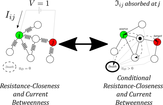
Figure 1: The relationship between current-based centralities and centralities using conditional current $\mathfrak{I}$. Even though resistance closeness and betweenness are different centralities, they can be described using the same electrical network (left). Likewise, the conditional resistance closeness and conditional current betweenness are described using the same random-walk process (right). When $\pi_{D}=0$, the conditional current and physical current are identical: $\mathfrak{I}=I$, and the left and right sides of the figure become equivalent, illustrating the isomorphism between random walks and resistor networks. On the left, the network currents are found according to Kirchhoff’s Laws. On the right, $\pi_{D}>0$, so $\mathfrak{I}\neq I$, and network currents are determined by counting edge traversals of random walkers (illustrated by the black disk) that do not land on the “death” node. The walker’s transition to the death node is controlled by the parameter $\pi_{D}$, while the transition probabilities to the network nodes are inversely proportional to the weighted degree of the node currently being occupied by the walker. The walker begins on the “source” node $i$ and ends on the “target” node $j$.

The shortest possible walk from $i$ to $j$ covers the weighted graph distance $d_{ij}$, so increasing $\pi_{D}$ tends to connect the walk with the centralities based on geodesics: betweenness and closeness. Walkers operating in the high $\pi_{D}$ regime are likely to die before making the full journey to a distant node, but the few walkers that survive will be overwhelmingly likely to have followed geodesics. Therefore, we restrict our attention to walkers that do not die, leading to a “conditional current” $\mathfrak{I}$ of walkers. In Sec. II.3.5, we provide an explicit formula for $\mathfrak{I}$ in terms of absorbing Markov matrices. The conditional current $\mathfrak{I}$, once substituted for the physical current $I$ in Eq. (5), provides a parametrized version of current-betweenness centrality, the conditional current-betweenness centrality. In Sec. II.3.6 we provide a calculation, also based on $\mathfrak{I}$, that parametrizes the resistance-closeness centrality, resulting in the conditional resistance-closeness centrality. With the restriction to conditional current, the parametrizations can reduce to the centralities discussed in the previous section at appropriate values of $\pi_{D}$: Conditional current-betweenness centrality reduces to current-betweenness centrality (as $\pi_{D}\to 0$) and betweenness centrality (as $\pi_{D}\to\infty$), while conditional resistance-closeness centrality reduces to resistance-closeness centrality and harmonic closeness centrality in the same limits, respectively.

Figure 1 illustrates the correspondence between resistor-network centralities and the parametrization controlled by $\pi_{D}$ and $\mathfrak{I}$. On the left side of the figure, resistance closeness and current betweenness are represented by the same diagram because both of those centralities can be calculated from current flows in the same resistor network. The parametrized forms of both these centralities are represented by the diagram on the right side of the figure.

The new centralities based on conditional current have a clear interpretation at intermediate parameter values. While as $\pi_{D}\to\infty$ the walker will only successfully follow geodesic paths, at smaller non-zero values of $\pi_{D}$ the walker will be restricted to short paths that are nearly geodesic. Finally, as $\pi_{D}$ goes to zero, the length of the walker’s paths will be completely unrestricted. Thus, $\pi_{D}$ can be said to tune the centralities’ preference for geodesic paths.

II.3.2 Specification of the interpolation parameter $\pi_{D}$

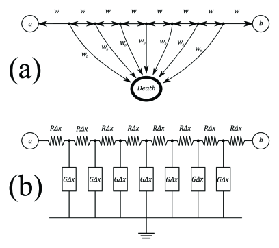
Figure 2: Weighted network edge from node $a$ to $b$ in (a) random-walk and (b) resistor-network descriptions. Case (b) is equivalent to a discrete approximation of a transmission line with constant resistance $R$ and ground conductance $G$ per unit length. In this figure, the number of intermediary edges, $n_{\mathrm{edge}}$, is 8. $\Delta x=d_{(a,b)}/n_{\mathrm{edge}}$.

Even though our two conditional current centralities are different measures, they are both based on the same random-walk dynamics controlled by the same parameter $\pi_{D}$. This random walk must be capable of reproducing the harmonic closeness centrality, which places an important requirement on its transition probabilities. In the case of weighted networks, the harmonic closeness centrality [see Eq. (2)] relies on the entries of the weighted adjacency matrix $\mathbf{A}$. Recall that, in closeness metrics, the inverse $(\mathbf{A}_{ab})^{-1}$ of an edge weight is generally associated with the length $d_{(a,b)}$ of that edge Opsahl et al. (2010). Therefore, the random-walk transition probabilities must be sensitive to the weights of edges as well.

To properly incorporate edge lengths (equivalently, inverse weights) into the absorbing random walk, we break each edge into a number of intermediary edges, connected by fictitious intermediary nodes, and then take the continuum limit. For example, Fig. 2(a) shows the edge $(a,b)$ broken into $n_{\mathrm{edge}}=8$ intermediary edges, connected by $n_{\mathrm{edge}}-1$ fictitious nodes. The weight of the entire edge is given by the adjacency matrix: $w_{(a,b)}=\mathbf{A}_{ab}=d_{(a,b)}^{-1}$. Therefore, an intermediary edge has weight

$$w=(d_{(a,b)}/n_{\mathrm{edge}})^{-1}=w_{(a,b)}*n_{\mathrm{edge}}.$$ (6)

In addition to its two connections along the original edge $(a,b)$, each intermediary node has an edge (weight $w_{D}$) to the absorbing “death” node. The behavior of $w_{D}$ as $n_{\mathrm{edge}}\to\infty$ is taken from an analogy with the lossy transmission line model from electrical power engineering Steer (2010). Fig. 2(b) depicts the lossy transmission line model with ground conductance per unit length $G$, line resistance per unit length $R$, and line inductance and ground capacitance set to zero. The correspondence between electrical networks and random walks Doyle and Snell (1984) implies that edge weights are proportional to conductances in the equivalent electrical network. If we take the proportionality factor to be one RExplained , $w_{D}=G\Delta x$ and $w=(R\Delta x)^{-1}$, where $\Delta x=d_{(a,b)}/n_{\mathrm{edge}}$. This means that edge weights (and hence, the adjacency matrix) have units of conductance, while edge lengths have units of resistance.

With intermediary edge weights in terms of $G$, in the continuum limit, we obtain random-walk transition probabilities $p_{\nu}$ over the edges $\nu$ incident on a given node $a$ (see Appendix A):

$$p_{\nu}(a)=\frac{[\sinh(\sqrt{GR}d_{\nu})]^{-1}}{N-1-k_{a}+\sum_{\mu}[\tanh(\sqrt{GR}d_{\mu})]^{-1}}.$$ (7)

Here, the index $\mu$ runs over all edges incident on $a$, $k_{a}$ is the unweighted degree of $a$, $d_{\nu}$ is the length of edge $\nu$, and $N$ is the number of nodes in the network. The probability of the walker on $a$ dying before successfully crossing an edge is therefore

$$p_{D}(a)=1-\frac{\sum_{\nu}[\sinh(\sqrt{GR}d_{\nu})]^{-1}}{N-1-k_{a}+\sum_{\mu}[\tanh(\sqrt{GR}d_{\mu})]^{-1}}.$$ (8)

Eqs. (7) and (8) are parametrized by the combination $\sqrt{GR}$, which has units of inverse length. In the theory of power transmission, $\sqrt{GR}$ is the inverse attenuation length of voltage signals along a lossy power line with negligible inductance and capacitance Steer (2010). For our purposes, $\sqrt{GR}$ is the parameter that controls the probability $p_{D}(a)$ of walker death at node $a$. In the next section, we show that increasing this parameter accomplishes the interpolations from resistance closeness to closeness and from current betweenness to betweenness. Thus, the centrality interpolation parameter is

$$\pi_{D}=\sqrt{GR}.$$ (9)

Eqs. (7) and (8) give sensible results for values of $\pi_{D}$ between $0$ and $\infty$. Table 1 summarizes the limiting values. In the limit $\pi_{D}\to 0$, the probabilities correctly reduce to those of a standard random walk.

Table 1: Walker transition probabilities for different values of $\pi_{D}$ in finite networks.

	$\lim{\pi_{D}\to\infty}$	$\pi_{D}>0$	$\lim{\pi_{D}\to 0}$
		Eq. (7)	(standard random walk)
$p_{\nu}(a)$	0	$\frac{[\sinh(\pi_{D}d_{\nu})]^{-1}}{\vphantom{\tilde{E}}N-1-k_{a}+\sum_{\mu}[\tanh(\pi_{D}d_{\mu})]^{-1}}$	$\frac{(d_{\nu})^{-1}}{\vphantom{\tilde{E}}\sum_{\mu}(d_{\mu})^{-1}}=\frac{w_{\nu}}{\vphantom{\tilde{E}}\sum_{\mu}w_{\mu}}$
		Eq. (8)
$p_{D}(a)$	1	$1-\frac{\sum_{\nu}[\sinh(\pi_{D}d_{\nu})]^{-1}}{\vphantom{\tilde{E}}N-1-k_{a}+\sum_{\mu}[\tanh(\pi_{D}d_{\mu})]^{-1}}$	0

With Eqs. (7) and (8) in place, we have completely described a model of the original network as a lossy resistor network. We have focused on the random-walk description of the resistor network to aid in the calculations of the following section. However, we stress that the description in terms of the electrical quantities $R$ and $G$ is equally valid. In fact, such a lossy resistor network would be physically realizable.

II.3.3 $\mathfrak{I}$ at extreme values of $\pi_{D}$

The entries of Table 1 are transition probabilities for a single walker step. They do not necessarily reflect what will happen in the conditional random walk, where we do not count walkers that die before reaching the target. In Sec. II.3.5, we derive a formula for calculating $\mathfrak{I}$ based on a surviving walker’s complete journey, not just a single step. However, we can already understand the behavior of $\mathfrak{I}$ at the limits of small and large $\pi_{D}$.

Figures 3(a) and 3(c) illustrate low-$\pi_{D}$ and high-$\pi_{D}$ conditional current $\mathfrak{I}$ on a weighted network representing the electrical power grid of the U.S. state of Florida Dale et al. (2009); Xu et al. (2014). Similarly, the first and last subfigure of Fig. 4 illustrates extremal $\mathfrak{I}$, as applied to a weighted network of social interactions in a group of kangaroos kan (2017); Grant (1973). These networks will be explained and studied in further detail in Sec. III; here they are just used to demonstrate the general behavior of conditional current. In the case of low $\pi_{D}$, $\mathfrak{I}$ spreads out exactly like physical current in a resistor network. In the case of high $\pi_{D}$, $\mathfrak{I}$ follows only weighted geodesic paths.

Employing our parametrization, Eqs. (3) and (5) undergo the transformation $I\longrightarrow\mathfrak{I}(\pi_{D})$ as $\pi_{D}$ is increased from zero. This naturally interpolates between the current-flow measure and the corresponding geodesic measure: between the resistance-closeness centrality [Eq. (3)] (as $\pi_{D}\to 0$) and the closeness [Eq. (2)] (as $\pi_{D}\to\infty$), and likewise between the current betweenness (or random-walk betweenness) (as $\pi_{D}\to 0$) [Eq. (5)] and the original betweenness [Eq. (4)] (as $\pi_{D}\to\infty$). To get a sense for why this is so, take $\lim_{\pi_{D}\to 0}$. In this case, when the “death probability” is zero, the walk reduces to the standard random walk on a weighted network. Such walks correspond to current flows as described in Sec. II.2: $\lim_{\pi_{D}\to 0}\mathfrak{I}(\pi_{D})=I$, which reproduces the centralities in Eqs. (3) and (5).

In the other direction, take a random walk with an extremely high $\pi_{D}$ and consider the effects on the the flow of walkers, $\lim_{\pi_{D}\to\infty}\mathfrak{I}(\pi_{D})$, from source $s$ to target $j$. Almost no such walks succeed in escaping from $s$ to $j$ before succumbing to the death probability $p_{D}$ from Table 1. Of the walkers that make this escape, the overwhelming majority will have taken walks along geodesics because even a single unnecessary step will incur a steep penalty from $\pi_{D}$. Furthermore, Eq. (27) in Appendix C shows that every geodesic path will get the same conditional current. Thus, $\lim_{\pi_{D}\to\infty}\mathfrak{I}_{sij}$ becomes proportional to $n_{sij}$, and the parametrized betweenness reduces to the standard betweenness in Eq. (4). (The more technical proof of the reduction of the parametrized resistance closeness to the harmonic closeness in Eq. (2) is presented at the end of Sec. II.3.6.)

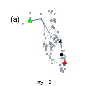
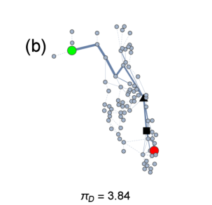
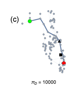
Figure 3: Conditional current flows $\mathfrak{I}$ at extreme and intermediate values of $\pi_{D}$ illustrated on the weighted Florida power-grid network (FLG) Xu et al. (2014). One unit of conditional current $\mathfrak{I}$ originates on the source node (green) and is absorbed at the target (red). Line thickness indicates conditional current magnitude, and edges with negligible conditional current ($<0.001$ units) are shown as dashed lines. The nodes marked with a square and a triangle are referred to in Sec. III.1.2 and Appendix D. (a) At $\pi_{D}=0$, $\mathfrak{I}$ is equal to physical current flow in a resistor network with the same topology as FLG: the current fans out over the network. (b) At $\pi_{D}=3.84$, $\mathfrak{I}$ begins to focus on shorter weighted paths. (c) At $\pi_{D}=10000$, $\mathfrak{I}$ is confined to the shortest weighted path from the source to the target. See the detailed discussion of this network in Sec. III.1.2.

The reduction of the conditional resistance closeness to the closeness and the conditional current betweenness to the betweenness are confirmed numerically for several example networks, as shown in Sec. III. We note that the reduction would not be possible without splitting weighted edges into intermediate edges and nodes with connections to the death node. Consider the alternative scheme where we capture edge weights in the random walk by dramatically increasing the transition probability for highly weighted edges and decreasing it for weakly weighted edges. In this case, the walker current would not be able to flow along geodesics that contain any long lines. For example, the geodesic in Fig. 3(c) contains a very long line incident on the node marked with a triangle. Even though this line is one of the longest (lowest weight) in the network, if the walker were to bypass it the conditional current would no longer flow along a geodesic, and the reduction to the closeness centrality would be impossible.

II.3.4 $\mathfrak{I}$ at intermediate values of $\pi_{D}$: tuning the preference for geodesic paths

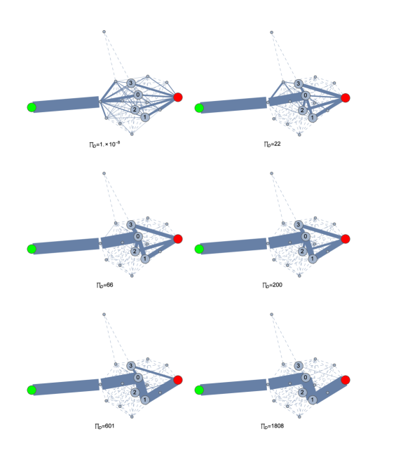
Figure 4: Conditional current at increasing values of $\pi_{D}$ illustrated on the weighted kangaroo social interaction network kan (2017); Grant (1973). Symbols have the same meanings as in Fig. 3. At values of $\pi_{D}$ near 0, $\mathfrak{I}$ is equal to the physical current flow in a resistor network, fanning out over all possible paths from source to target. As $\pi_{D}$ approaches $\infty$, $\mathfrak{I}$ follows only the shortest weighted path. In the intermediate $\pi_{D}$ regime, $\mathfrak{I}$ splits among three approximately equal-length paths, passing through nodes 1, 2, and 3, respectively. All of these paths pass through node 0. As $\pi_{D}$ increases, more and more $\mathfrak{I}$ flows along the shortest of these paths. See further discussion in Sec. III.1.2 and Sec. III.2.2.

Figure 4 shows the conditional currents $\mathfrak{I}$ on a weighted network representing social interaction in a group of kangaroos kan (2017); Grant (1973). It includes the full range of conditional current behavior, including intermediate parameter values. As discussed in Sec. II.3.1, the smaller $\pi_{D}$ the longer the paths the random walker is able to explore. In the figure, at low values of $\pi_{D}$ the conditional current splays out over the network: the walker is able to take advantage of many parallel paths from the start to the target, whether they are short or long. As $\pi_{D}$ increases, fewer and fewer of the long parallel paths can be followed. Finally, at large $\pi_{D}$, the conditional current becomes negligible for all but the geodesic path, and all parallelism is suppressed. In this way, the parameter tunes the conditional current’s preference for geodesic (and nearly-geodesic) paths. The centralities based on this conditional current will probe the network at the level of parallelism specified by the value of the parameter $\pi_{D}$. (Note that $\pi_{D}$ does not simply tune the conditional current’s preference for short paths, since the walker’s start and target nodes may be an arbitrary distance apart. )

II.3.5 Calculating $\mathfrak{I}$ vs $\pi_{D}$: conditional current betweenness

For values of $\pi_{D}$ between 0 and $\infty$, the conditional current $\mathfrak{I}(\pi_{D})$ of walkers must be calculated using the theory of absorbing Markov Chains Novotny (2001); Iosifescu (1980). Take the random-walk matrix $\mathbf{W}$, whose elements $\mathbf{W}_{mn}$ indicate the single-step transition probability from node $m$ to $n$, and partition it according to a form which picks out absorbing and transient nodes. In the present case, there are two absorbing nodes: the first is a sink that corresponds to the death probability $p_{D}$, while the second is the “target” node where the conditional current leaves the network: node $j$ in the calculation of $\mathfrak{I}_{ij}(\pi_{D})$. The walkers begin on node $i$. The canonical form for $\mathbf{W}$ is

$$\mathbf{W}=\begin{pmatrix}\boldsymbol{\mathbb{I}}&\boldsymbol{\mathbb{O}}\\ \begin{pmatrix}\ket{\mathscr{A}^{\mathrm{sink}}}&\ket{\mathscr{A}^{\mathrm{target}}}\end{pmatrix}&\mathbf{T}\end{pmatrix}.$$ (10)

Here, $\mathbf{T}$ is the $(N-1)\times(N-1)$ transient transition matrix, whose elements are transition probabilities between the non-absorbing (transient) states. $\boldsymbol{\mathbb{O}}$ is the $2\times(N-1)$ matrix of zeroes, indicating that walkers cannot make transitions from absorbing states to transient states. Here, $\boldsymbol{\mathbb{I}}$ is the $2\times 2$ identity matrix, indicating that a walker in an absorbing state is stuck there forever. The two $(N-1)$-dimensional column vectors $\ket{\mathscr{A}}$ describe absorption transitions to the sink and the target node, respectively. An element of the $\mathbf{T}$ matrix $\mathbf{T}_{mn}$ is given by $[1-p_{D}(m)](\mathbf{A}_{mn}/A_{m})$, according to the standard definition of random walks on a network with adjacency matrix $\mathbf{A}$ Doyle and Snell (1984), modified by the walker death probability $p_{D}(m)$ from Eq. (8). (Recall that $A_{m}$ is the weighted degree of node $m$.) Similarly, $(\mathscr{A}^{\mathrm{target}})_{m}$, the $m$th entry of $\ket{\mathscr{A}^{\mathrm{target}}},$ equals $(1-p_{D}(m))(\mathbf{A}_{mj}/A_{m})$, while $(\mathscr{A}^{\mathrm{sink}})_{m}$ is just $p_{D}(m)$.

A key object in the theory of absorbing random walks is the fundamental matrix $\mathbf{F}$, given by

$$\mathbf{F}=(\boldsymbol{\mathbb{I}}-\mathbf{T})^{-1}.$$ (11)

$\mathbf{F}_{in}$ is the expected number of times a walker starting on source $i$ can make it to $n$ before being absorbed by the sink. Because the target node $j$ is not transient, $n\neq j$. Define the unbolded variable $F_{in}$ similarly to $\mathbf{F}_{in}$, but now allowing $n$ to take on the value of $j$. By the properties of the fundamental matrix,

$$F_{in}=\begin{cases}\mathbf{F}_{in}&n\neq j\\ \sum_{m\sim n}\mathbf{F}_{im}\mathscr{A}^{\mathrm{target}}_{m}&n=j\end{cases},$$ (12)

where the sum is over the neighbors of $n$, and node $j$ is the target of the random walk.

The random-walk formulation can be connected to the current-flow formulation by extrapolating from the well-known Doyle and Snell (1984) isomorphism for the case $\pi_{D}=0$. In that case, the edge current produced by a unit voltage is proportional to the net number of walker crossings: the number in the forward direction, minus the number in the reverse direction. The proportionality constant is the inverse of the resistance distance, $(R^{\mathrm{eff}}_{i\,j})^{-1}$, which describes the total number of walkers released from the node maintained at unit voltage. To generalize the resistance-closeness centrality of Eq. (3) to non-zero values of $\pi_{D}$, $R^{\mathrm{eff}}_{ij}$ must deviate from its value at $\pi_{D}=0$, so the proportionality constant is unknown. Thus, in the $\pi_{D}>0$ regime, we must work with ratios of currents so that the constant does not appear. Recall that, for $\pi_{D}>0$, the current is conditional on reaching target $j$; we denote this condition as “$\mid j$”. Equation (12) can be used to formulate $\mathfrak{I}_{i(a,b)j}$: the current entering the network at $i$, eventually flowing through the edge $(a,b)$, and finally leaving the network at $j$ (i.e., not succumbing to $\pi_{D}$):

$$\begin{array}[]{ccccc}\frac{\mathfrak{I}_{i(a,b)j}}{\mathfrak{I}_{ij}}&=&\mathbb{E}\small(\mbox{\# walker crosses from $a$ to $b$ $\mid$ $j$})&-&\mathbb{E}\small(\mbox{\# walker crosses from $b$ to $a$ $\mid$ $j$})\\ &=&F_{i\;a}\mathbf{T}_{a\;b}F_{b\;j}/F_{i\;j}&-&F_{i\;b}\mathbf{T}_{b\;a}F_{a\;j}/F_{i\;j}\end{array}.$$ (13)

Here, every term has an implicit dependence on $\pi_{D}$, and the $\mathbb{E}(*\mid j)$ are conditional expectation values. The above equation is just the “$\mid j$” conditional version of a well-known connection between walker paths and electric currents (see, e.g., Newman (2005)). Note that this expression for conditional current satisfies Kirchhoff’s Current Law, since the path of any individual walker must do so.

Equation (13) only provides ratios of conditional currents $\mathfrak{I}$. However, in the betweenness centrality of Eq. (5), the currents $I$ are found in ratios as well. The above can be used to calculate the interpolated betweenness currents by summing the edge currents into a given node, as in Sec. II.2.2: $\mathfrak{I}_{sij}/\mathfrak{I}_{sj}=\sum_{a:\mathfrak{I}_{s(a,i)j}>0}\mathfrak{I}_{s(a,i)j}/\mathfrak{I}_{sj}$. This process leads to a parametrized form of the current-betweenness centrality: conditional current-betweenness centrality in Table 2.

Table 2: Current betweenness, betweenness, and intermediate centralities. The top-left entry defines current-betweenness centrality (equivalent to random-walk centrality Newman (2005)), while the top-right entry defines betweenness centrality in an analogous form. The interpolation between these two centralities in terms of the “death parameter” $\pi_{D}$ is described by the top-middle entry. The middle row indicates the corresponding values of $\pi_{D}$. The bottom row describes the type and behavior of the current corresponding to each parameter value.

Current Betweenness	$\longleftarrow$ Interpolation$\longrightarrow$	Betweenness
[see Eq. (5)]	Conditional Current Betweenness	[see Eq. (4)]
$\mathbf{M}^{\mathrm{CBT}}_{ij}=\sum_{s}I_{sij}/I_{sj}$	$\mathbf{M}^{\mathrm{CBT}}_{ij}(\pi_{D})=\sum_{s}\mathfrak{I}_{sij}(\pi_{D})/\mathfrak{I}_{sj}(\pi_{D})$	$\mathbf{M}^{\mathrm{BET}}_{ij}=\sum_{s}n_{sij}/g_{sj}$
$\lim_{\pi_{D}\to 0}$	$\pi_{D}>0$	$\lim_{\pi_{D}\to\infty}$
$I_{ij}$	$\mathfrak{I}_{ij}(\pi_{D})$	$\mathfrak{I}$ only flows on geodesics:
(physical current)	(conditional current)	$\mathfrak{I}_{sj}\propto g_{sj}$ and $\mathfrak{I}_{sij}\propto n_{sij}.$

II.3.6 Conditional resistance closeness: calculating the $\pi_{D}$-parametrized effective resistance

To naively parametrize the form of the resistance-closeness centrality in Eq. (3) would require the values $\mathfrak{I}_{ij}(\pi_{D})$, which cannot be determined from Eq. (13). This is because the absorbing random walk outlined above, for $\pi_{D}>0$, does not correspond to a physical current, and thus only current ratios are determined.

To bridge the gap, we seek to determine which edge resistances—given the same network topology—would reproduce the calculated conditional current as a physical current: $I=\mathfrak{I}$. If we could obtain a set of resistances $\{R^{\mathfrak{I}}_{\nu}\}$ that would reproduce the set of conditional currents $\{\mathfrak{I}_{\nu}\}$ as physical currents, then the corresponding voltage drop $V_{i\,j}$ from $i$ to $j$ would simply be equal to $\sum_{\nu\in\mathcal{P}}\mathfrak{I}_{\nu}R^{\mathfrak{I}}_{\nu}$, where the edge index $\nu$ runs over the edges in any oriented path $\mathcal{P}$ from $i$ to $j$. (Note that in general when $I\neq\mathfrak{I}$, $V_{\nu}\neq\mathfrak{I}_{\nu}R^{\mathfrak{I}}_{\nu}$.)

From $V_{i\,j}=I_{i\,j}R^{\mathrm{eff}}_{i\,j}$, the voltage drop for a unit current is equal to the effective resistance. Hence, it is convenient to set the total conditional current (from $i$ to $j$) to unity.

$$R^{\mathrm{eff}}_{i\,j}=\sum_{\nu\in\mathcal{P}}\mathfrak{I}_{\nu}R^{\mathfrak{I}}_{\nu}.\hskip 20.00003pt(\mathrm{for}\;\mathfrak{I}_{ij}=I_{ij}=1)$$ (14)

With $I_{i\,j}=\mathfrak{I}_{i\,j}$ set to unity, the edge current $\mathfrak{I}_{\nu}$ over edge $\nu=(a,b)$ becomes $\mathfrak{I}_{\nu}=\mathfrak{I}_{i(a,b)j}/\mathfrak{I}_{i\,j}=\mathfrak{I}_{i(a,b)j}$. (Even though we are dealing with undirected networks, consistency with what follows forces us to specify edge orientation explicitly, meaning that $\mathfrak{I}_{(a,b)}=-\mathfrak{I}_{(b,a)}$.)

Unfortunately, the values $\{R^{\mathfrak{I}}_{\nu}\}$ (and hence, also the value of $R^{\mathrm{eff}}_{i\,j}$) are under-determined by the currents in Eq. (13). This can be seen from the following linear condition on $\{R^{\mathfrak{I}}_{\nu}\}$ Bollobás (1998), which is equivalent to Kirchhoff’s Voltage Law :

$$\forall r:\sum_{\nu}\mathbf{K}_{r\,\nu}\mathfrak{I}_{\nu}R^{\mathfrak{I}}_{\nu}=0.$$ (15)

Here, $\mathbf{K}$ is the reduced cycle matrix, describing the edges that form a maximal collection of linearly independent cycles on the network. The index $r$ denotes independent oriented cycles, and $\mathbf{K}_{r\,\nu}$ is non-zero only for network edges $\nu$ participating in cycle $r$. Thus, the possible edge resistances $\{R^{\mathfrak{I}}_{\nu}\}$ form the (generally multidimensional) null-space of the matrix $[\mathbf{K}_{r\,\nu}\mathfrak{I}_{\nu}]$, with the added physical constraint that $R^{\mathfrak{I}}_{\nu}\geq 0,\forall\nu$. For a network with $N$ nodes and $M$ edges, the matrix $[\mathbf{K}_{r\,\nu}\mathfrak{I}_{\nu}]$ has dimensions $(M-N+1)\times M$. Using this equation, it can be verified that sometimes wildly different resistance distributions can lead to the same current flow on a given network.

Nonetheless, it is possible to compute a uniquely suitable set of resistances $\{R^{\mathfrak{I}}_{\nu}\}$, given two common-sense criteria: (1) Because increasing $\pi_{D}$ serves to inhibit current, we constrain the resistances $R^{\mathfrak{I}}_{\nu}$ to be larger than or equal to their $\pi_{D}=0$ values; i.e., $R^{\mathfrak{I}}_{\nu}\geq R^{\mathrm{orig}}_{\nu},\forall\nu$. (2) Because any vector in the null-space of $[\mathbf{K}_{r\,\nu}\mathfrak{I}_{\nu}]$ remains in the null-space after scaling, there is no upper bound on the effective resistance $R^{\mathrm{eff}}_{i\,j}=V_{i\,j}$, and thus, we define the $\pi_{D}$-parametrized effective resistance $\mathfrak{R}_{ij}$ to be the minimum value of $R^{\mathrm{eff}}_{ij}$.

To find $\mathfrak{R}_{ij}$, we minimize the expression in Eq. (14), requiring that a valid solution $\{R^{\mathfrak{I}}_{\nu}\}$ must satisfy condition (1) and Eq. (15):

$$\underset{\{R^{\mathfrak{I}}_{\nu}\}}{\text{minimize}} \sum_{\nu\in\mathcal{P}}\mathfrak{I}_{\nu}R^{\mathfrak{I}}_{\nu}$$

subject to $$\sum_{\mathclap{\nu}}\begin{aligned} \mathbf{K}_{r\,\nu}\mathfrak{I}_{\nu}R^{\mathfrak{I}}_{\nu}=0&,&\forall&\;\mathrm{independent\;cycles}\;r\\[12.91663pt] R^{\mathfrak{I}}_{\nu}\geq R^{\mathrm{orig}}_{\nu}&,&\forall&\;\mathrm{edges}\;\nu\\[12.91663pt] \end{aligned}$$ (16)

Note that $\mathfrak{I}$ depends on $i,j,$ and $\pi_{D}$. Even though the first sum is over the edges in the arbitrary path $\mathcal{P}$, the minimization is over all the edges in the network. $\mathfrak{R}_{ij}$ is the minimized objective function.

Finding $\{R^{\mathfrak{I}}_{\nu}\}$ that satisfies the above is a standard linear programming problem, which is guaranteed to be feasible, as shown in Appendix B. Because the problem is feasible (and clearly bounded), the optimal solution $\mathfrak{R}_{ij}$ is, in principle, calculable. Techniques such as the simplex method Murty (1983) and interior point methods Boyd and Vandenberghe (2004) are generally used to find this optimal solution. As a practical matter, the linear programming algorithms struggle to find solutions when conditional currents $\mathfrak{I}_{\nu}$ become too small. The difficulty is overcome by removing low-current edges from the network, since they do not contribute to $\mathfrak{R}_{ij}$ anyway. For the networks under consideration, once low-current edges are removed, the convergence is fast and the particular choice of linear solver is not important noteSolver .

Finally, the optimized value $\mathfrak{R}$ of the linear programming problem in Eq. (16), given conditional currents calculated from Eq. (13), leads to a parametrized form of the resistance-closeness centrality of Eq. (3): the conditional resistance-closeness centrality . See Table 3.

We can now understand the behavior of the conditional resistance closeness as $\pi_{D}\rightarrow\infty$. In this limit, conditional current becomes restricted to the shortest path $\mathcal{P^{*}}$ from source $i$ to target $j$. Setting $\mathcal{P}=\mathcal{P^{*}}$ in Eq. (14), $R^{\mathrm{eff}}_{i\,j}=\sum_{\nu\in\mathcal{P^{*}}}\mathfrak{I}_{\nu}R^{\mathfrak{I}}_{\nu}$. Because we are dealing with unit current, and because there is only one shortest path (see Appendix C.3),

$$\lim_{\pi_{D}\to\infty}R^{\mathrm{eff}}_{i\,j}=\sum_{\nu\in\mathcal{P^{*}}}R^{\mathfrak{I}}_{\nu}.$$ (17)

The final centrality is calculated using $\mathfrak{R}_{ij}$ . The sum in Eq. (17) is clearly minimized, within our constraints, by setting $R^{\mathfrak{I}}_{\nu}=R^{\mathrm{orig}}_{\nu}=d_{\nu}$, for all $\nu\in\mathcal{P^{*}}$. The current can be forced to match the conditional current by setting $R_{\nu}^{\mathfrak{I}}=\infty$ for all $\nu\notin\mathcal{P^{*}}$, but this does not affect $\mathfrak{R}_{ij}$. Thus,

$$\lim_{\pi_{D}\to\infty}\mathfrak{R}_{ij}=\sum_{\nu\in\mathcal{P^{*}}}d_{\nu}=d_{ij}.$$ (18)

Inverting this effective resistance, as in the top-middle entry of Table 3, results in the formula for harmonic closeness, as in the top-right entry of the table.

Table 3: Resistance closeness, harmonic closeness, and intermediate centralities. The presentation is similar to that of Table 2.

Resistance Closeness	$\longleftarrow$ Interpolation$\longrightarrow$	Harmonic Closeness
[see Eq. (3)]	Conditional Resistance Closeness	[see Eq. (2)]
$\mathbf{M}^{\mathrm{RCC}}_{ij}={1}/{R^{\mathrm{eff}}_{ij}}=I_{ij}$	$\mathbf{M}^{\mathrm{RCC}}_{ij}(\pi_{D})=1/{\mathfrak{R}_{ij}(\pi_{D})}\;\mbox{\;and Eq. }(\ref{linprog})$	$\mathbf{M}^{\mathrm{HCL}}_{ij}={1}/{d_{ij}}$
$\lim_{\pi_{D}\to 0}$	$\pi_{D}>0$	$\lim_{\pi_{D}\to\infty}$
$I_{ij}$	$\mathfrak{I}_{ij}(\pi_{D})$	$\mathfrak{I}$ only flows on
(physical current)	(conditional current)	geodesics from $i$ to $j$.

II.3.7 The conditional walker-flow centralities

In summary, we have shown that the parameter $\pi_{D}$ interpolates between the leftmost and rightmost columns in Tables 2 and 3. The transition is from current-betweenness centrality at $\pi_{D}=0$ to betweenness centrality as $\pi_{D}$ approaches $\infty$ (Table 2), and from resistance-closeness centrality at $\pi_{D}=0$ to the harmonic closeness centrality as $\pi_{D}$ approaches $\infty$ (Table 3). Intermediate parameter values tune the closeness and betweenness centralities’ preference for geodesic paths and, as a result, probe the network’s behavior at different levels of parallelism.

The new centralities that interpolate between these limits may be called conditional walker-flow centralities. The measures in Table 2 are connected to each other by the same random-walk process that connects the measures in Table 3, reinforcing the idea that all four centralities in those tables are part of the natural class of walker-flow centralities. Stephenson’s information centrality Stephenson and Zelen (1989) and Newman’s random-walk betweenness Newman (2005) also belong to this class, having been proved equivalent to resistance closeness and current betweenness, respectively.

III Conditional Walker-Flow Centrality Results

III.1 Results on example networks

We now apply the conditional current centralities developed in the previous section to four example networks, demonstrating the interpolations and limits summarized in Tables 2 and 3. The networks are chosen to have different edge densities and types of edge weighting: the kangaroo network is dense and has integer weights, the karate club network has intermediate density and is unweighted, and the power-grid network is sparse with continuous weights. (We also study the unweighted version of the power-grid network for comparison.) The characteristics of the example networks, as well as literature references and the figure numbers of corresponding results, are summarized in Table 4.

Table 4: Example network summary. Networks have $N$ nodes and $M$ edges. The density of a network is defined as the number of edges divided by the number of possible edges: $M/(0.5N(N-1))$. See text for discussion.

Network	Refs.	N	M	Density	Weights	Results
Kangaroo Group	kan (2017); Grant (1973)	17	91	0.67	Integer	Fig. 5
Zachary Karate Club	Zachary (1977)	34	78	0.14	Unweighted	Fig. 6
Weighted Power Grid	Xu et al. (2014); Dale et al. (2009)	84	137	0.04	Continuous	Figs. 7, 9, and 10
Unweighted Power Grid	Xu et al. (2014); Dale et al. (2009)	84	137	0.04	Unweighted	Figs. 8, and 9

III.1.1 Overview of numerical results

The values of the conditional walker-flow centralities—the conditional current betweenness and the conditional resistance closeness—are presented in Figs. 5-8. There, each line represents the centrality results of a different node across a range of values of the dimensionless parameter $\pi_{D}\langle L\rangle$, where $\langle L\rangle$ is the average edge length (edge resistance) of the network.

The large circles in the plots show that the conditional walker-flow centralities correspond to the limiting centralities in Tables 2 and 3, regardless of weighting type. As an example, consider the conditional current-betweenness centrality for the kangaroo network, Fig. 5(a). The circles on the left side of the figure correspond to the current-betweenness centrality. Those on the right correspond to the weighted betweenness centrality, obtained with a weighted version of the algorithm from Brandes (2001). In the limits, the lines coincide with the circles, showing that the conditional current betweenness reduces to the current betweenness at low $\pi_{D}$ and to the standard weighted betweenness at high $\pi_{D}$. Similarly, Fig. 5(b) shows that the conditional resistance closeness reduces to the resistance closeness at low $\pi_{D}$ and to the harmonic closeness at high $\pi_{D}$.

As discussed in Sec. II.1, the figures in this section depict the unnormalized centrality values produced by our algorithms. This enables us to better compare centralities across different values of $\pi_{D}$. In the normalized version, an increase in node $i$’s centrality may create a spurious decrease in the centrality of node $j$, even if the conditional currents through $j$ remain unchanged.

\begin{overpic}[unit=1mm,scale={.8},trim=0.0pt 0.0pt 0.0pt 0.0pt,clip]{fig_kanga_bet_lines.eps}\end{overpic}

\begin{overpic}[unit=1mm,scale={.8},trim=0.0pt 0.0pt 0.0pt 0.0pt,clip]{fig_kanga_cond_res_lines.eps}\end{overpic}

Figure 5: Conditional walker-flow centrality of every node in the kangaroo network. Each line represents the unnormalized centrality of a different node. In this and the following figures, the abscissa is made dimensionless by multiplying $\pi_{D}$ by $\langle L\rangle$, the average edge length (edge resistance) of the network. Here, $\langle L\rangle\approx 0.432$. (a) Conditional current betweenness. The circles on the left and right ends show the values of the current-betweenness centrality and the betweenness centrality, respectively. Note that some nodes on the periphery of the network have a centrality value of zero. The data are thus represented on a semi-logarithmic scale. (b) Conditional resistance closeness. The circles on the left and right ends show the values of the resistance-closeness centrality and the harmonic closeness centrality, respectively. The data are represented on a log-log scale.

\begin{overpic}[unit=1mm,scale={.8},trim=0.0pt 0.0pt 0.0pt 0.0pt,clip]{fig_karate_bet_lines.eps}\put(0.0,62.0){\bf\large}\end{overpic}

\begin{overpic}[unit=1mm,scale={.75},trim=0.0pt 0.0pt 0.0pt 0.0pt,clip]{fig_karate_cond_res_lines.eps}\put(0.0,62.0){\bf\large}\end{overpic}

Figure 6: Conditional walker-flow centrality of every node in the karate-club network. See the caption to Fig. 5 for explanatory details. All centrality values are unnormalized. Because this network is unweighted, $\langle L\rangle=1$. (a) Conditional current betweenness. The curve marked with a star is referenced in Sec. III.3 and in Appendix D. (b) Conditional resistance closeness. The plateau region between $\pi_{D}\langle L\rangle\approx 1$ and $\pi_{D}\langle L\rangle\approx 100$ occurs because $\pi_{D}$ is large enough to pick out (possibly multiple) shortest paths in the original network but not yet large enough to resolve the unique shortest path created by the introduction of random noise. See further discussion in Appendix C.3.

\begin{overpic}[unit=1mm,scale={.8},trim=0.0pt 0.0pt 0.0pt 0.0pt,clip]{fig_florida_weighted_bet_lines.eps}\end{overpic}

\begin{overpic}[unit=1mm,scale={.75},trim=0.0pt 0.0pt 0.0pt 0.0pt,clip]{fig_florida_weighted_cond_res_lines.eps}\end{overpic}

Figure 7: Conditional walker-flow centrality of every node in the weighted power-grid network. See the caption to Fig. 5 for explanatory details. All centrality values are unnormalized. In this network, $\langle L\rangle\approx 0.067$. (a) Conditional current betweenness. (b) Conditional resistance closeness.

\begin{overpic}[unit=1mm,scale={.8},trim=0.0pt 0.0pt 0.0pt 0.0pt,clip]{fig_florida_unweighted_bet_lines.eps}\end{overpic}

\begin{overpic}[unit=1mm,scale={.75},trim=0.0pt 0.0pt 0.0pt 0.0pt,clip]{fig_florida_unweighted_cond_res_lines.eps}\end{overpic}

Figure 8: Conditional walker-flow centrality of every node in the unweighted power-grid network. See the caption to Fig. 5 for explanatory details. All centrality values are unnormalized. Because this network is unweighted, $\langle L\rangle=1$. (a) Conditional current betweenness. (b) Conditional resistance closeness. The plateau region is similar to that described in the caption to Fig. 6.

III.1.2 Numerical results for individual networks

We next remark on some particulars of the results for the different example networks.

Kangaroo network. The first network under consideration is a weighted network of social interactions within a group of 17 kangaroos kan (2017); Grant (1973). The nodes represent individual animals, and the 91 weighted edges represent their social interactions. The weights are integers indicating the number of observed interactions. This network is illustrated in Fig. 4.

Figure 5 depicts the conditional walker-flow centralities for this network. In part (a), the conditional current betweenness behavior of two nodes stands out. Consider the nodes with the two highest values of the standard betweenness (the two dots at the top-right of the figure). These correspond to the nodes marked “0” and “1” in Fig. 4. For a broad range of $\pi_{D}$ values, these have much higher conditional current betweenness than any other node. At $\pi_{D}\langle L\rangle\lessapprox 20$, their centrality values become close to those of several other nodes. We have remarked that $\pi_{D}$ tunes the conditional current-betweenness centrality’s preference for geodesic paths (see Sec. II.3.4). Thus, Fig. 5(a) shows that at tuning level indicated by $\pi_{D}\langle L\rangle\lessapprox 20$, the network structure ceases to prioritize the two nodes in question. In fact, they rank only number four and five in current-betweenness centrality. A similar sensitivity to resolution is not observed in the conditional current-closeness centralities in Fig. 5(b). Such large, non-monotonic variations in the conditional current betweenness are analyzed in Sec. III.3.

Karate club network. The second network under consideration is Zachary’s karate club Zachary (1977). The nodes represent the 34 members of the club. The 78 unweighted edges of the network represent the presence of social interactions between club members. This is a standard test case in network science. Fig. 6 shows that the two nodes representing the club’s instructor and administrator have the highest conditional walker-flow centralities across all values of $\pi_{D}$. Thus, unlike the two kangaroo network nodes discussed previously, the two club officials’ high centrality rank does not depend on the centrality’s preference for geodesic paths. This is consistent with the non-monotonicity analysis of Sec. III.3, where we explain why unweighted networks are less susceptible to large changes in centrality. In such a network, nodes with a clear centrality lead in the extreme $\pi_{D}$ limits are likely to keep their high centrality rank in the intermediate regime.

Power-grid networks. The last two networks under consideration are based on the map of the Florida power grid obtained from Dale et al. (2009) and studied in Xu et al. (2014). The 84 nodes represent high-capacity generators and important substations of the Florida power grid in 2009. The 137 edges represent power transmission lines. This network is illustrated in Fig. 3, and walker-flow centrality results are reported in Figs. 7-8. We analyzed both a weighted (Fig. 7) and an unweighted (Fig. 8) version of this network. The unweighted version only captures the presence or absence of transmission lines. In the weighted version, edge weights are real numbers proportional to the estimated total conductance of the direct connection between two nodes. Specifically, the edge weight between nodes $a$ and $b$ is equal to the number of transmission lines divided by the geographical distance between $a$ and $b$, as in Abou Hamad et al. (2011).

In both the weighted and unweighted cases, a single node (marked with a triangle in Fig. 3) stands out as having the highest centrality across a broad range of parameter values. This node corresponds to an electrical substation with one of the largest degrees in the network. Standard betweenness centrality tends to pick out bottlenecks, and while the node in question does find itself in a bottleneck region of the network, it also has unusually long connections, which link geographically different regions of the graph. In fact, this node lies at the intersection of multiple communities in high-modularity partitions of the power grid network by different methods Abou Hamad et al. (2010, 2011). In addition, another node (marked with a square in Fig. 3) exhibits striking behavior in the intermediate $\pi_{D}$ regime in Fig. 7(a). This node, having the second-highest centrality at $\pi_{D}\left<L\right>\approx 0.5$, is not assigned high centrality in either the betweenness or the current-betweenness limits. Thus, it is only important at moderate levels of parallelism. Both of the salient nodes in the weighted power-grid network will be studied further in Sec. III.3, which discusses non-monotonic behavior in the conditional current-betweenness centrality.

III.2 Degenerate and nearly-degenerate paths

In addition to providing insight about specific networks, the numerical results presented in this section help us understand the workings of conditional current more clearly. In particular, we discuss the properties of the conditional current in the presence of degenerate and nearly-degenerate paths in the network.

III.2.1 Degenerate and semi-degenerate paths

The conditional walker-flow centralities exhibit noteworthy behavior in the presence of degenerate and semi-degenerate paths. (We consider two paths semi-degenerate if they have the same weighted length but different unweighted lengths.) In the case of degenerate paths, at large $\pi_{D}$ the conditional current betweenness reproduces the potentially huge combinatorial weighting that is a consequence of the definition of the standard betweenness centrality. Because the conditional current calculations do not explicitly consider the combinatorics of possible paths, it is noteworthy that the conditional betweenness can still reduce to the standard betweenness in such edge cases. In the case of semi-degenerate paths, convergence to the betweenness centrality sometimes requires a slight modification to the walk matrix $\mathbf{W}$ used to calculate $\mathfrak{I}$ in Eqs. (10-13). See further details in Appendix C.

III.2.2 Nearly degenerate paths: $\pi_{D}$ controls path-length resolution

In Sec. II.3.4, we demonstrated that as we decrease $\pi_{D}$ from $\infty$ to $0$, the conditional current $\mathfrak{I}$ will prefer geodesic paths less and less. Our numerical studies lead to an illuminating interpretation of this behavior: $\pi_{D}$ tunes the conditional walker-flow centralities’ ability to distinguish between paths of similar weighted length. In this view, the centralities always prefer nearly geodesic paths, and $\pi_{D}$ controls which path lengths count as “nearly” geodesic. At high $\pi_{D}$, only the true geodesics qualify. As $\pi_{D}$ decreases, longer and longer parallel paths from the start to the target will be indistinguishable from geodesics.

This resolution-tuning effect is illustrated in Fig. 4, where $\mathfrak{I}$ flows from a specific start node (green) to a specific target node (red). There, at $\pi_{D}=66$, almost all of $\mathfrak{I}$ passes through three similarly long paths, each of which goes through node 0. The shortest path goes through node 1, with a weighted length of 1.481. The paths through 2 and 3 have weighted lengths of 1.486 and 1.483, respectively. For comparison, the path that goes directly from 0 to the target node has a weighted length of 1.6. At $\pi_{D}=66$, the centralities can resolve length differences between the direct 0-to-target path and the other three paths. However, it cannot yet resolve the smaller differences between the paths through 1, 2, and 3, so these three paths have nearly equal values of $\mathfrak{I}$. As the parameter value increases to $\pi_{D}=601$, the centralities begin to distinguish between these three paths, and $\mathfrak{I}$ through node 2 is nearly eliminated. As $\pi_{D}$ grows even larger, all of $\mathfrak{I}$ will pass through the node-1 path, which is the shortest start-target path in the network.

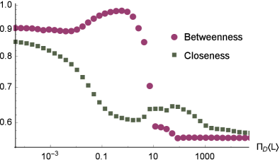
Figure 9: Pearson correlations of weighted with unweighted network versions of walker-flow centralities on the Florida power-grid network. The conditional current-betweenness centrality is represented by circles, while the conditional resistance-closeness centrality is represented by squares. Both correlations tend to get larger as $\pi_{D}$, and hence the path-length resolution level, gets smaller. When the centralities are less sensitive to differences in edge weights, the differences between the weighted and unweighted networks are diminished. The conditional current-betweenness correlation maximum occurs at the same value of $\pi_{D}\langle L\rangle$ that produces the large bump in maximum centrality in Fig. 7 because, in the unweighted power-grid network, there is a large gap between the maximum centrality and the other nodes’ centralities (see Fig. 8).

The resolution-tuning interpretation of $\pi_{D}$ explains the similarity of the current betweenness and resistance closeness on weighted and unweighted versions of the same network. In Fig. 9 we present the Pearson correlations of the conditional walker-flow centralities on the weighted Florida power-grid network with those on the unweighted network, across a large range of $\pi_{D}$ values. (For two centrality measures $c$ and $c^{\prime}$ on a given network, the correlation is calculated using $\sum_{i}(c_{i}-\langle c\rangle)(c^{\prime}_{i}-\langle c^{\prime}\rangle)/(N\sigma_{c}\sigma_{c^{\prime}})$, where the sum runs over all nodes $i$.) For both the conditional current betweenness and the conditional resistance closeness, the correlations tend to increase for smaller values of $\pi_{D}$. At smaller $\pi_{D}$ the centralities are less sensitive to differences in edge weights, so the differences between the weighted and unweighted networks are diminished, and the correlations become large. In the intermediate range, betweenness is almost independent of the weighting (high correlation), while closeness is quite strongly affected (low correlation).

The resolution-tuning effect also has practical implications for helping the conditional resistance-closeness centrality converge to the harmonic closeness, in the case of unweighted networks. The method involves adding a small amount of random noise to the edge weights of the network—not enough to substantially affect centrality values at low and intermediate values of $\pi_{D}$. This method is explained more fully in Appendix C.3. Note that we do not need to add the random noise when calculating the conditional current-betweenness centrality, since in that case, degenerate paths must be included for the centrality to correctly reduce to the betweenness centrality.

III.3 Non-monotonicity

III.3.1 Complex behavior in the conditional walker-flow centralities

Figs. 5(a), 6(a), 7(a), and 8(a) show that the conditional current betweenness can exhibit complex behavior over the full range of $\pi_{D}$, including non-monotonicity, pronounced maxima and minima, and line crossings that indicate changes in the centrality rankings. The general reason is that, being based on a conserved walker current, betweenness is a limited resource. Though the conditional current centrality curves are complex, they are produced by a simple process: the tuning behaviors described in Sec. II.3.4 . The tuning is generally monotonic in the sense that increasing $\pi_{D}$ takes conditional current from indirect paths and re-routes it along more direct paths (see Fig. 4). Sec. III.2.2 provides an alternate interpretation of the same tuning process, where the underlying monotonicity can be seen even more clearly. From that perspective, as $\pi_{D}$ is reduced from $\infty$ the walker-flow centralities monotonically reduce the length resolution with which they identify shortest paths. The complex, non-monotonic behaviors seen in the figures emerge from the aggregate of many such simple processes and from the uneven distribution of the conserved walker current.

The behavior of the conditional resistance-closeness centrality [Figs. 5(b), 6(b), 7(b), and 8(b)] is much more regular than that of the conditional current betweenness. Generally, the conditional resistance closeness decreases with increasing $\pi_{D}$. This is because increasing $\pi_{D}$ restricts parallel paths of conditional current as in Fig. 4, which leads to higher resistance values in the linear programming procedure of Sec. II.3.6, and thus to lower closeness. The main exceptions to this trend are the small centrality spikes seen in Figs. 5(b) and 7(b), which are discussed in Appendix C.2.

III.3.2 How non-monotonicity in the conditional current betweenness arises in bottlenecks

Much of the complex behavior of the conditional current-betweenness centrality can be described as non-monotonicity. Non-monotonic behavior is evident in Figs. 5(a), 6(a), 7(a), and 8(a). The figures show that the most important nodes often exhibit such non-monotonic behavior—for example the two high-centrality power-grid nodes discussed in Sec. III.1.2. Thus, understanding the non-monotonicity becomes crucial.

\begin{overpic}[unit=1mm,scale={.8},trim=0.0pt -14.22636pt 0.0pt 0.0pt,clip]{FLNonmon.eps}\end{overpic}

\begin{overpic}[unit=1mm,scale={.545},trim=0.0pt 0.0pt 0.0pt 0.0pt,clip]{FLPart.eps}\end{overpic}

Figure 10: Non-monotonicity and partitioning of the weighted Florida power-grid network. (a) The conditional current-betweenness centrality curves from Fig. 7(a) that show pronounced non-monotonicity. (b) Node colors indicate membership in the partitions found using the Kernighan–Lin algorithm. The large, numbered nodes correspond to the curves in (a). See further details in Appendix D.

It is noteworthy, then, that in our numerical examples, every single node with relatively pronounced non-monotonicity (relative to the network’s other nodes) lies at a bottleneck. For example, consider Fig. 10, which describes the weighted power-grid network. Part (a) reproduces the curves exhibiting pronounced non-monotonicity in Fig. 7(a). Part (b) shows the network nodes divided into two equally-sized partitions using the Kernighan–Lin algorithm Newman (2004). This is a greedy algorithm for finding partitions that minimize the sum of the (weighted) lengths of inter-partition edges, meaning that these edges are bottlenecks between the two halves of the network. (Since the algorithm uses a random start, we took the best partitioning obtained in 1000 runs.) All the most non-monotonic nodes are bottleneck nodes: they either lie at the boundary between partitions, or are directly connected to such nodes noteOnDownstream . This includes nodes 3 and 7, which are the two high-centrality nodes mentioned earlier (depicted as a triangle and square, respectively, in Fig. 3).

This result is very general. In the three other example networks, the nodes with the highest non-monotonicity are always found at—or adjacent to—the partition boundary. This can even occur for non-central nodes and ones with low absolute non-monotonicity. For example, the node corresponding to the starred curve in Fig. 6 lies on the partition boundary of the karate club network. Furthermore, the exact partitioning method is not important: we obtain the same behavior with partitions derived from the first nontrivial Laplacian eigenvector Abou Hamad et al. (2010). In Appendix D, we quantify the non-monotonicity of centrality curves and provide a complete listing of the most non-monotonic nodes in the example data.

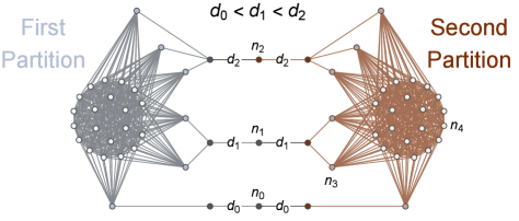
Figure 11: Example network leading to non-monotonic conditional current-betweenness. Hue indicates membership in the partitions found using the Kernighan–Lin algorithm. Node lightness/darkness encodes the connection pattern: the lightest nodes form two complete subnetworks of size $N_{C}$. The nodes of intermediate lightness have connections to all nodes in the nearest complete subnetwork. The darkest nodes have only a few connections, and thus form bottlenecks. Edge lengths are labeled with $d$’s. Unlabeled edges all have the same length $d_{\mathrm{other}}$.

The non-monotonic behavior of nodes on the partition boundary can be understood with reference to the idealized network of Fig. 11. There, as in Fig. 10, we have two (nearly) equally sized partitions separated by a few bottleneck nodes. Most of each partition is made up of a complete subnetwork of size $N_{C}$. Because $N_{C}$ is large, most of the conditional current betweenness is due to current flowing between the complete subnetworks. The non-monotonicity in node $n_{1}$ is caused by a trade-off between number of paths and path length. The most direct paths between subnetworks take only 6 steps. Of these, there are 4 paths through $n_{1}$ and 9 paths through $n_{2}$ for every path through $n_{0}$. This biases the conditional current betweenness to assign more centrality to node $n_{2}$ and less to $n_{0}$. However, the lengths of all these direct paths are slightly different because $d_{0}\lessapprox d_{1}<d_{2}<d_{\mathrm{other}}$, which introduces an opposite bias. The effect is that, as $\pi_{D}$ is decreased from $\infty$ to $0$, the centrality of $n_{1}$ first rises, then falls.

\begin{overpic}[unit=1mm,scale={.8},trim=0.0pt 0.0pt 0.0pt 0.0pt,clip]{artificial_graph_resultsA.eps}\end{overpic}

\begin{overpic}[unit=1mm,scale={.8},trim=0.0pt 0.0pt 0.0pt 0.0pt,clip]{artificial_graph_resultsB.eps}\end{overpic}

Figure 12: Conditional current betweenness for the network in Fig. 11. (a) The vertical coordinates of the dashed lines are in the ratio 1:4:9, equal to the number of short paths from left cluster to right cluster passing through $n_{0}$, $n_{1}$, and $n_{2}$, respectively. For the same reason, the vertical coordinates of the two circles are in the ratio 1:4. The horizontal coordinates of the circles correspond to the smallest $\pi_{D}$ where the centrality of $n_{2}$ is minimal. The large values of $N_{C}$ and $d_{\mathrm{other}}$ are chosen so that the data approach this ratio in the intermediate $\pi_{D}$ regime. The curves thus exhibit non-monotonic behavior, by design. See the text for discussion. (b) Even at more realistic values of $N_{C}$ and $d_{\mathrm{other}}$, the non-monotonic behavior is qualitatively similar.

This can be understood more specifically using the resolution tuning concept (Sec. III.2.2) and the observation that, at high $\pi_{D}$, the centrality reproduces the path counting of the standard betweenness (Sec. III.2.1 and Appendix C.1). The details of these considerations are borne out by the numerical results in Fig. 12(a). At very high values of $\pi_{D}$ (right-most plateaus in the figure), current flows mostly over the shortest weighted path, which goes through $n_{0}$. As a result, $n_{1}$ and $n_{2}$ have lower betweenness. As $\pi_{D}$ is decreased, the centrality reaches a resolution level where $d_{0}$ and $d_{1}$ are indistinguishable, but both are still distinguishable from $d_{2}$ and $d_{\mathrm{other}}$, so the betweenness of $n_{2}$ is still low. Here, because there are 4 times as many paths through $n_{1}$ as $n_{0}$, the centrality of the former is about 4 times as big. (See the circles in the figure, which are placed on the horizontal axis just before $n_{2}$’s centrality begins to rise. The vertical coordinates are in the ratio of 4:1.) As $\pi_{D}$ is decreased even further, $d_{1}$, $d_{2}$, and $d_{3}$ are all indistinguishable from each other, but still distinguishable from $d_{\mathrm{other}}$. Hence, the betweenness values for $n_{0}$, $n_{1}$, and $n_{2}$ are close to the ratio 1:4:9 (as indicated by the dashed lines). The centrality rank of $n_{1}$ goes from third, to first, to second. Because of current conservation, this means that the centrality curves exhibit extrema noteOnMaximum and are thus non-monotonic.

In Fig. 12(a), we chose large values of $N_{C}$ and $d_{\mathrm{other}}$ to match the above theoretical betweenness ratios (encoded by the circles and dashed lines). However, as shown in part (b) of the figure, the qualitative features of (a)—especially the non-monotonicity—persist even with more realistic parameters. We propose that the cause of non-monotonicity in the real example networks is qualitatively the same as that in the idealized network of Fig. 11. That is, non-monotonicity is caused by the competition of different-length and differently-connected paths between large network communities. In realistic networks, there may be more than two large communities and more than three paths between them, resulting in more complex non-monotonic behavior than is seen in Fig. 12. Nonetheless, the real networks studied here accord with the non-monotonicity model of Fig. 11, including the placement of non-monotonic nodes on partition boundaries, as well as the reduced occurrence of non-monotonicity in non-weighted graphs (Figs. 6 and 8), which are less likely to have small differences in path-length.

These considerations can shed light on the behaviors of the high-centrality nodes described in Sec. III.1.2. In our examples, large changes in centrality are almost always consequences of non-monotonicity, so unweighted networks are more likely to have stable centralities. This is exactly what happens in the (unweighted) karate club network (Fig. 6), where the two highest-centrality nodes maintain their rank across the entire range of $\pi_{D}$.

Figure 12 also gives insight into two types of nodes that are not high-centrality bottlenecks. The first, $n_{3}$, does not have the highest centrality rank at any value of $\pi_{D}$. Furthermore, it does not lie on the network’s partition boundary. However, it is directly connected to $n_{1}$, which does lie on the boundary. As a result, $n_{3}$ receives half of that node’s walker current, and therefore inherits its non-monotonicity as well. This is analogous to nodes 4, 5, 6, and 7 in Fig. 10, which inherit the non-monotonicity from node 3, which has much higher centrality than any other in the intermediate $\pi_{D}$ regime. Second, $n_{4}$ is a node that lies within a community, far from the partition boundary. Therefore, it has an entirely monotonic centrality curve, much like the monotonic nodes of the kangaroo network and weighted power-grid network, seen in Figs. 5(a) and 7(a), respectively.

IV Conclusion

We have shown that the class of walker-flow centralities includes important and commonly known centrality measures. The walker-flow centralities that are most frequently encountered in the literature admit a natural parametrization scheme, based on the walker death parameter $\pi_{D}$, which interpolates between the measures in the left and right columns of Tables 2 and 3. Our conditional current-betweenness centrality interpolates from random-walk betweenness (equivalently, current betweenness) at $\pi_{D}=0$ (no walker death), to standard betweenness as $\pi_{D}\to\infty$ (walker death likely). Our conditional resistance-closeness centrality interpolates from harmonic information centrality (equivalently, resistance closeness) at $\pi_{D}=0$, to harmonic closeness as $\pi_{D}\to\infty$. We believe our absorbing walker-flow method is the first to interpolate simultaneously across both the betweenness and the closeness continua.

The interpolating centralities are also meaningful at intermediate values of $\pi_{D}$. As $\pi_{D}$ increases from zero, the centralities prioritize geodesic and nearly-geodesic paths. Therefore, parallelism in the network becomes less and less important. Finally, as $\pi_{D}\to\infty$, parallel paths between any pair of nodes are ignored (unless they have degenerate lengths). From this perspective, $\pi_{D}$ can be seen as a tuning parameter that sets the centralities’ preference for geodesic paths and thus the level of parallelism. This can be informative of the structure of specific networks, since some centrality features only appear in limited $\pi_{D}$ regimes. For example, in Sec. III.1.2, we discuss how a particular node in the Florida power-grid network becomes important only in the intermediate $\pi_{D}$ regime. Generally, non-monotonic behavior of conditional current betweenness in the intermediate $\pi_{D}$ regimes is found in nodes that lie close to a community boundary, which experience a competition between (a) lying on many paths and (b) lying on short paths.

We have argued that considering the entire range of $\pi_{D}$ can be revealing about a network’s structure, but it can also be useful to pick out a single “best” parameter value for a given network. In previous work on the Florida power-grid network Xu et al. (2014); Gurfinkel et al. (2015), we found a strong correlation between the known generation capacities of power plants and the values of a centrality based on Estrada’s communicability Estrada and Hatano (2008); Estrada et al. (2009). The best-fit parameter in the communicability centrality can be viewed as a measure of a length scale inherent in the network. In future reports, we will describe how several different centrality measures also reveal the same length scale. We similarly plan to use centrality-matching to reveal “best” values of $\pi_{D}$.

The present work has focused on general features of the centralities’ numerical results. These reveal a second effect of the interpolation parameter: in addition to controlling geodesic-path preference, it controls the centralities’ path-length resolution ability. At low values of $\pi_{D}$, the centralities cannot distinguish between geodesic and nearly geodesic paths. This implies that standard current betweenness and resistance closeness centralities, obtained at $\pi_{D}=0$, are not sensitive to small variations in edge weights in complex networks, as seen in Fig. 9. Our method provides versions of betweenness and closeness centralities with an adjustable resolution level.

Appendix A Derivation of Eqs. (7) and (8)

Consider the absorbing random walk on a chain of $n_{\mathrm{edge}}-1$ intermediary nodes depicted in Fig. 2(a). The situation describes a random walker attempting to cross a long edge $(a,b)$ with constant death probability at every intermediary node. The walker begins on the first intermediary node to the right of $a$ and can absorb on $a$ (transmission failed), $b$ (transmission succeeded), and the “death” node (walker died). Here, the difference between transmission failure and walker death is that, in the former case, the walker can try again: a new transmission attempt will start on some edge $(a,c)$, where $c$ is a neighbor of $a$ in the original network. Standard random-walk dynamics require that the death probability at every intermediary node be $p=w_{D}/(w_{D}+2w)$, while the probability of moving along each of the two intermediary edges is $w/(w_{D}+2w)$. [See Eq. (6) and the following sentence for the definitions of $w$ and $w_{D}$.]

The probability of successful transmission in a single attempt, $p_{T}(a,b)$, is found using standard methods Logan (2013). We solve the following linear difference relation for $p_{T;k}$, the probability of transmission over $(a,b)$ given a start on intermediary node $k$:

$$p_{T;k}=\frac{1-p}{2}p_{T;k-1}+\frac{1-p}{2}p_{T;k+1}$$ (19)

Let $k=0$ correspond to node $a$ and $k=n_{\mathrm{edge}}$ correspond to node $b$. The boundary conditions become $p_{T;0}=0$ and $p_{T;n_{\mathrm{edge}}}=1$. This leads to

$$p_{T}=p_{T;1}=\frac{2}{1-p}\frac{\sqrt{2p-p^{2}}}{\left(\frac{1+\sqrt{2p-p^{2}}}{1-p}\right)^{n_{\mathrm{edge}}}-\left(\frac{1-\sqrt{2p-p^{2}}}{1-p}\right)^{\vphantom{E^{E}}n_{\mathrm{edge}}}},$$ (20)

where $p$ is a function of $w$ and $w_{D}$.

To obtain the continuum limit, $n_{\mathrm{edge}}$ will increase to infinity. Therefore, $w$ and $w_{D}$ must be described in terms of quantities per unit length. Analogy with the lossy transmission line model from power engineering Steer (2010) suggests these quantities to be the ground conductance per unit length, $G$, and the line resistance per unit length, $R$. The correspondence between electrical networks and random walks Doyle and Snell (1984) then implies that $w_{D}=G\Delta x$ and $w=(R\Delta x)^{-1}$, where $\Delta x=d_{(a,b)}/n_{\mathrm{edge}}$.

Expansion in terms of $\Delta x$ results in

$$p_{T}(a,b)=\frac{\sqrt{GR}\,\Delta x}{\sinh({d_{(a,b)}\sqrt{GR})}}+\mathcal{O}(\Delta x^{2}).$$ (21)

Reversing the boundary conditions for Eq. (19) results in $p_{R}(a,b)$, the probability that the walker will return to $a$ before reaching $b$:

$$p_{R}(a,b)=1-\frac{\sqrt{GR}\,\Delta x}{\tanh({d_{(a,b)}\sqrt{GR})}}+\mathcal{O}(\Delta x^{2}).$$ (22)

As remarked earlier, $p_{T}(a,b)$ and $p_{R}(a,b)$ describe only a single attempt at transmission over the edge $(a,b)$. The final transmission probability $p_{(a,b)}$ can include failed attempts to reach any nearest neighbor of $a$; so long as the walker returns to $a$ rather than dying, it can try again. What matters is that the ultimately successful transmission occurs over $(a,b)$. This reasoning is captured in the recursive equation

$$p_{(a,b)}=k_{a}^{-1}\left(\sum_{l\sim a}p_{R}(a,l)p_{(a,b)}+p_{T}(a,b)\right).$$ (23)

Here, the sum is over nearest neighbors of $a$ and the inverse unweighted degree factor $k_{a}^{-1}$ comes from the random choice of the first edge the walker attempts to cross.

Solving the linear equation (23) for $p_{(a,b)}$ and substituting the lowest-order terms from Eqs. (21) and (22) results in

$$p_{(a,b)}=\frac{[\sinh(\sqrt{GR}\,d_{(a,b)})]^{-1}}{\sum_{l\sim a}[\tanh(\sqrt{GR}\,d_{(a,l)})]^{-1}}.$$ (24)

Note that the dependence on the granularity parameter $\Delta x$ has canceled out. This cancellation further justifies the use of the physically-motivated parameters $G$ and $R$ in the per-step death probability $p$: the cancellation does not occur if we instead choose a constant death probability per unit length.

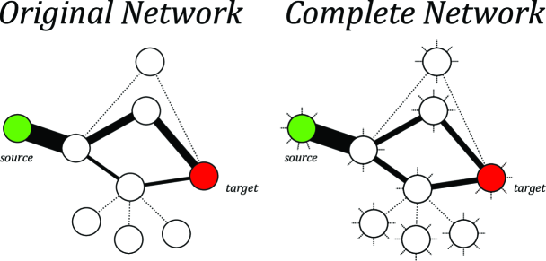
Figure 13: Conditional current flow in the case of degenerate shortest paths in an unweighted network. The conserved walker current from “source” to “target” in a simple example graph is illustrated for large $\pi_{D}$ ($\pi_{D}=1000)$. Edge current magnitude is proportional to line thickness, and infinitesimal current is depicted with dotted lines. Conditional current $\mathfrak{I}$ flows only on shortest paths from “source” to “target”. If (left side) transmission probabilities are given by Eq. (24), then less current will flow on geodesics that contain higher-degree nodes. When transmission probabilities are given by Eq. (25) (right side), all degenerate geodesics carry equal currents because all nodes have degree $N-1$. In this case the network is described by a complete graph, but the edges not present in the original network have infinite length and, therefore, no conditional currents.

A final consideration is that Eq. (24) leads to unwanted behavior in the case of unweighted networks with degenerate (equal length) paths. Figure 13 (left) shows the conditional current $\mathfrak{I}$ in a simple example-network for large values of $\pi_{D}=\sqrt{GR}$. The figure illustrates that while $\mathfrak{I}$ is restricted to geodesics, it is smaller for paths that include higher-degree nodes. The solution is to replace all non-edges in the network with edges of infinite length. In effect, this gives all nodes the same unweighted degree of $N-1$. As a result, degenerate geodesics will share equal conditional currents, as shown in Fig. 13 (right). (However, we continue to use $k_{a}$ to refer to the unweighted degree of node $a$: $k_{a}=\sum_{l\sim a}1$.) With this change, Eq. (24) becomes

$$p_{(a,b)}=\frac{[\sinh(\sqrt{GR}\,d_{(a,b)})]^{-1}}{N-1-k_{a}+\sum_{l\sim a}[\tanh(\sqrt{GR}\,d_{(a,l)})]^{-1}},$$ (25)

which leads to Eqs. (7) and (8).

Appendix B Feasibility of the linear programming problem for $\mathfrak{R}$

To show that the linear programming problem of Eq. (16) is feasible is to show that there exists a solution $\{R^{\mathfrak{I}}_{\nu}\}$ that does not necessarily minimize $R^{\mathrm{eff}}$. If a node potential mapping $\{V^{\mathfrak{I}}_{l}\}$ can be found to reproduce the conditional currents as physical currents, $I=\mathfrak{I}$, then $\sum_{r}\mathbf{K}_{r\,\nu}\mathfrak{I}_{\nu}R^{\mathfrak{I}}_{\nu}=0$ is trivially satisfied for all independent cycles $r$ because $\mathfrak{I}_{\nu}R^{\mathfrak{I}}_{\nu}$ is edge $\nu$’s potential drop $V^{\mathfrak{I}}_{\nu}$, and the sum of potential drops around a cycle must be zero. Indeed, the condition in question is just a re-statement of Kirchhoff’s Voltage Law.

A directed acyclic graph always admits a topological ordering $\mathcal{O}$ on the nodes, such that any directed edge $\nu=(a,b)$ satisfies $\mathcal{O}_{a}>\mathcal{O}_{b}$ (edges point from higher to lower order). Below, we prove that the conditional current $\mathfrak{I}$ results in a directed acyclic graph. The topological ordering obtained from the graph of $\mathfrak{I}$s can be converted into a consistent potential mapping by assigning $V^{\mathfrak{I}}_{a}>V^{\mathfrak{I}}_{b}$ whenever $\mathcal{O}_{a}>\mathcal{O}_{b}$. The value of $R^{\mathfrak{I}}_{\nu}$ is then chosen to satisfy $V^{\mathfrak{I}}_{\nu}=V^{\mathfrak{I}}_{a}-V^{\mathfrak{I}}_{b}=\mathfrak{I}_{\nu}R^{\mathfrak{I}}_{\nu}$. Finally, the potential of every node can be scaled to ensure that $R^{\mathfrak{I}}_{\nu}\geq R^{\mathrm{orig}}_{\nu}$ for all $\nu$, and Eq. (16) is proven feasible.

The conditional current mapping clearly defines a directed graph. We show that the resulting graph is acyclic through contradiction. Assume that nodes $k$ through $k+m-1$ form a directed cycle of $m$ edges, such that $\mathfrak{I}$ flows from $l$ to $l+1$ for $l\in[k,k+m-1]$. (Because this is a cycle, nodes $l$ and $l+m$ are equivalent.) The previous statement, in light of Eq. (13), becomes

$$\begin{array}[]{ccccc}F_{i\;l}\mathbf{T}_{l\;l+1}F_{l+1\;j}&>&F_{i\;l+1}\mathbf{T}_{l+1\;l}F_{l\;j}&&\\ &\Updownarrow&&\\ F_{i\;l}\frac{[\sinh(\sqrt{GR}\,d_{(l,l+1)})]^{-1}}{g(l)}F_{l+1\;j}&>&F_{i\;l+1}\frac{[\sinh(\sqrt{GR}\,d_{(l+1,l)})]^{-1}}{g(l+1)}F_{l\;j}&&\\ .\end{array}$$ (26)

for all $l\in[k,k+m-1]$. Here, $\mathbf{T}$ is substituted from Eq. (7), from which we define $g(l)=N-1-k_{l}+\sum_{\mu}[\tanh(\sqrt{GR}d_{\mu})]^{-1}$, where the sum runs over edges incident on node $l$. Noting that $d_{(l,l+1)}=d_{(l+1,l)}$, the above can be rewritten as $f(l)>f(l+1)$ where $f(l)=F_{i\;l}\left(g(l)F_{l\;j}\right)^{-1}$. The inequalities form a chain: $f(l)>f(l+1)>\cdots>f(l+m)=f(l)$, which is a contradiction. Therefore, $\mathfrak{I}$ always results in a directed acyclic graph.

Appendix C Degenerate and semi-degenerate paths

C.1 Degenerate paths

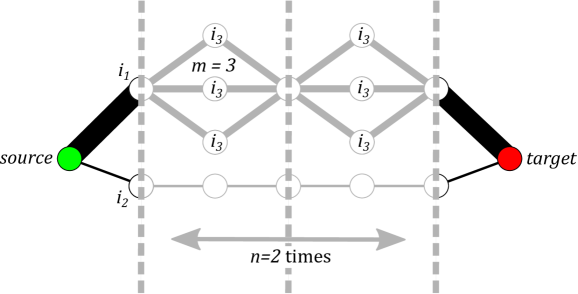
Figure 14: Example unweighted network with many degenerate paths from source to target. The graph distance between the source and target nodes is $2(n+1)$. There are $m^{n}$ times as many geodesics of this length passing through node $i_{1}$ as there are through node $i_{2}$. Because $n_{\mathrm{source},i,\mathrm{target}}$ in the betweenness formula [Eq. (4)] counts the total number of geodesics passing through $i$, the contribution to $i_{1}$’s betweenness centrality from this (source, target) pair is $m^{n}$ times the contribution to $i_{2}$’s betweenness. Our conditional current-betweenness centrality reproduces this result at large values of $\pi_{D}$. Here, $m=3$ and $n=2$ is illustrated. Line thicknesses are proportional to the number of geodesic paths along an edge, as well as the conditional current at large $\pi_{D}$. Node $i_{3}$ can be taken to be any of the $mn$ nodes in that position, and is discussed further in the text.

In the case of many degenerate paths, the standard betweenness centrality [Eq. (4)] can exponentially prefer some nodes over others, even when they both lie on geodesics. Consider the example network in Fig. 14. There, geodesics between the source and target nodes have graph distance $2(n+1)$. However, there are $m^{n}$ times as many geodesics passing through node $i_{1}$ as there are through node $i_{2}$. Because $n_{\mathrm{source},i,\mathrm{target}}$ in the betweenness formula counts the total number of geodesics passing through $i$, the contribution to $i_{1}$’s betweenness centrality from this (source, target) pair is $m^{n}$ times the contribution to $i_{2}$’s betweenness.

The conditional current-betweenness centrality reproduces this behavior at large $\pi_{D}$, without having been explicitly designed to do so. Because all the nodes in the network lie on geodesics, no nodes will have zero conditional current $\mathfrak{I}$. However, $\mathfrak{I}$ through $i_{1}$ is $m^{n}$ times as large as $\mathfrak{I}$ through $i_{2}$, so the relative contributions to current betweenness are the same as they are in standard betweenness. In that case, by symmetry and conditional current conservation, $\mathfrak{I}$ through $i_{3}$ is $m^{(n-1)}$ times as large as $\mathfrak{I}$ through $i_{2}$, where $i_{3}$ can be any of the $mn$ nodes compatible with the position of $i_{3}$ in the figure. In the other extreme, at low $\pi_{D}$, the conditional current is more evenly shared. At $\pi_{D}=0$, the conditional current becomes identical with the physical current on the corresponding resistor network. In the large $n$ limit, this means that $\mathfrak{I}$ through $i_{3}$ is identical to $\mathfrak{I}$ through $i_{2}$, while $\mathfrak{I}$ through $i_{1}$ is $m$ times as large.

C.2 Semi-degenerate paths

Consider two paths of the same weighted length $d_{\mathrm{path}}$ from source $i$ to target $j$, and calculate $\mathfrak{I}$ in the high $\pi_{D}$ limit. If the two paths also have the same unweighted length, $\mathfrak{I}$ will be equal on the two paths. However, if the paths have different unweighted lengths (are semi-degenerate), $\mathfrak{I}$ will not be equal. This can be seen from the formula for transition probability along edge $\nu$ [Eq. (7)] which, in the high $\pi_{D}$ limit, reduces to $p_{\nu}=\exp(-\pi_{D}d_{\nu})/(N-1)$. In this limit, the conditional current $\mathfrak{I}_{\mathrm{path}}$ along a (weighted) shortest path is proportional to the product of edge transition probabilities along the path. Therefore,

$$\mathfrak{I}_{\mathrm{path}}\propto\exp(-\pi_{D}d_{\mathrm{path}})/(N-1)^{n_{\mathrm{path}}},$$ (27)

where ${n_{\mathrm{path}}}$ is the number of non-fictitious nodes along the path.

Eq. (27) means that, in the high $\pi_{D}$ limit, while conditional current will flow along a path if and only if it is a weighted shortest path, more conditional current will flow along the paths that involve the fewest nodes. Occasionally, this can lead to conditional current betweenness failing to converge to betweenness in the high $\pi_{D}$ limit. The only example of this in our numerical studies can be seen for the integer-weighted kangaroo network in Fig. 5(a), where in the bottom right corner, one data-point indicating non-zero betweenness does not match up with the corresponding conditional current betweenness curve, which goes to zero.

In principle, this convergence problem for semi-degenerate paths can only occur in weighted networks (in unweighted networks $d_{\mathrm{path}}=n_{\mathrm{path}}$). Furthermore, it cannot occur for continuously weighted networks because it is overwhelmingly unlikely that two different paths would have precisely the same weighted length. For the same reason, the convergence of the conditional resistance distance is unaffected, since in this case the addition of a small amount of random noise effectively creates a continuously weighted network. Of all realistic networks, the problem primarily occurs in networks that have integer edge lengths, up to a constant factor. One way around this difficulty is to introduce macroscopic intermediary nodes such that, after the addition of the new nodes, every edge has the same length. [Unlike the microscopic intermediary nodes of Sec. II.3.2, the macroscopic nodes are included in the walk matrix $\mathbf{W}$ of Eq. (10). However, since they are not real network nodes, they are not included in the centrality matrix $\mathbf{M}$ of Eq. (1).] This effectively transforms the integer-weighted network into an unweighted network, which removes any issues with semi-degenerate paths. However, finding a single version of our conditional current that gives correct results for all types of weighted networks is a priority for future research.

The conditional walker-flow centralities also prefer shorter unweighted paths in the case of merely approximate semi-degeneracy, though this does not affect convergence to the limiting centralities (betweenness, current betweenness, closeness, and resistance closeness). Consider a network with only two paths from $i$ to $j$; path 1 has a slightly longer weighted length than path 2, but a shorter unweighted length. The two paths are thus approximately semi-degenerate. When $\pi_{D}$ is low enough that the difference between the two weighted lengths cannot be resolved, path 1 will carry more conditional current $\mathfrak{I}$. As the centrality’s resolution increases with $\pi_{D}$, more and more of the conditional current will flow along path 2. At some value of $\pi_{D}$, $\mathfrak{I}$ will be equal across the two paths. At this point, the effective resistance $\mathfrak{R}_{ij}$ will be lowest because $\mathfrak{I}$ mimics current flow for two resistors in parallel. In networks with more than two paths, a similar phenomenon causes the small spikes in nodes’ resistance closeness, as can be seen in Figs. 5(b) and 7(b).

C.3 Random noise ensures reduction of conditional resistance-closeness to closeness

Table 3 shows that, for the conditional resistance-closeness to reduce to the harmonic closeness centrality at high $\pi_{D}$, $\mathfrak{R}_{ij}$ must equal $d_{ij}$ in that parameter regime. Since unweighted networks generally have multiple equal length (degenerate) paths between a given source $i$ and target $j$, the linear programming method assigns a value of effective resistance $\mathfrak{R}_{ij}$ lower than that of the graph distance $d_{ij}$—parallel paths lower the resistance. We thus add a small amount of random noise to every edge weight, changing the network from unweighted (i.e., unit edge weights) to weighted. This creates a single shortest path from $i$ to $j$, whose length is approximately $d_{ij}$. Therefore, at large values of $\pi_{D}$, we find $\mathfrak{R}_{ij}\approx d_{ij}$. The amount of random noise is too small to be resolved at anything but very large values of $\pi_{D}$, so it does not affect our results when $\pi_{D}$ is not large. At large values of $\pi_{D}$, the noise is resolved, and the centrality reduces to closeness centrality.

The resolution-tuning effect of $\pi_{D}$ is evident in the plateau regions in Figs. 6(b) and 8(b), for example between $\pi_{D}\langle L\rangle\approx 1$ and $\pi_{D}\langle L\rangle\approx 100$ in Fig. 8(b). In such plot regions, where most of the curves are approximately constant, even as $\pi_{D}$ increases the differences in path lengths are not large enough to be resolved by the centrality. The end of the plateau in Fig. 8(b) corresponds to the value of $\pi_{D}$ at which the centrality is capable of resolving the random noise.

Without the addition of random noise, the plateaus would extend to arbitrarily large values of $\pi_{D}$. The resulting centrality can be viewed as an alternative closeness measure, where only shortest paths contribute, but the presence of degenerate paths is taken into account and makes the source and target “closer”. This is because the alternative closeness considers flows rather than single travelers. The harmonic closeness does not distinguish between situations in which there is a unique shortest path of length $l$ and where there are many degenerate shortest paths of length $l$.

Appendix D Non-monotonicity data tables

In Sec. III.3, we explained how non-monotonicity in the conditional current betweenness arises in nodes that experience a competition between (a) lying on many paths and (b) lying on short paths. To quantify the non-monotonicity of centrality curves $f(\pi_{D})$, we rely on the Lack of Monotonicity (LOM) index Davydov and Zitikis (2017), a functional given by

$$\mathrm{LOM}(f(x))=2\min\left(\int_{0}^{\infty}(f^{\prime}(x))^{+}\mathrm{d}x,\left|\int_{0}^{\infty}(f^{\prime}(x))^{-}\mathrm{d}x\right|\right).$$ (28)

The $+$ and $-$ superscripts pick out, respectively, the positive and negative part of a function $g$. Specifically, $(g(x))^{+}=\max(g(x),0)$ and $(g(x))^{-}=\min(g(x),0)$. A monotonic function results in a LOM of 0, while heavily non-monotonic functions have large LOM.

Tables 5-8 list the nodes in the four example networks in order of decreasing LOM for the conditional current betweenness, along with the nodes’ relationships to the partition boundary. For every network, we list up to the 10 highest-LOM nodes—so long as the LOM is above zero. The nodes with the top-ranked LOM index invariably appear on the partition boundary. The nodes in the top 5% of LOM rankings appear either on the boundary or adjacent to it.

All the partition boundaries in the tables are found using the Kernighan–Lin algorithm. As discussed in Sec. III.3, the presence of high LOM nodes on or near partition boundaries is reproduced with an alternative partitioning scheme based on the smallest non-trivial eigenvector of the graph Laplacian (the Fiedler vector). The alternative partitioning is a modified form of the standard Laplacian partitioning Newman (2010): a constant is added to every element of the Fiedler vector to ensure partitions with equal (or approximately equal) numbers of nodes. The relationship between non-monotonic nodes and boundaries is not observed for partitioning methods that do not produce two equally-sized partitions—such as the unmodified Laplacian method and the multi-community islanding method from Abou Hamad et al. (2011). This may be because the conditional current betweenness (see Table 2) assigns equal weight to all source/target pairs $(s,j)$. Bottlenecks between two equally-sized partitions will experience the most conditional current flow once all pairs are accounted for, similar to the bottlenecks in Fig. 11.

Table 5: Non-monotonicity data for the kangaroo network. Of the 9 nodes not appearing in the table, all have zero LOM. Of these, 2 are not boundary nodes. (Because of the tight-knit network structure, all of the network’s nodes are either on or adjacent to the partition boundary. )

LOM Index	Partition	Boundary Node	Boundary Neighbor
22.09	2	YES	NO
20.70	1	YES	NO
16.17	1	YES	NO
14.27	2	YES	NO
3.43	2	YES	NO
0.69	1	YES	NO
0.10	1	YES	NO
0.01	1	YES	NO

Table 6: Non-monotonicity data for the karate club network. Of the 32 nodes not appearing in the table, all have zero LOM. Of these, 21 are not boundary nodes. (Because of the tight-knit network structure, all but one of the network’s nodes are either on or adjacent to the partition boundary.) The highest-LOM node is denoted with a star in Fig. 6.

LOM Index	Partition	Boundary Node	Boundary Neighbor
17.92	2	YES	NO
9.20	1	YES	NO

Table 7: Non-monotonicity data for the weighted power-grid network. Of the 74 nodes not appearing in the table, 51 have non-zero LOM (mean 472.96), and 28 of these are neither boundary nodes nor boundary neighbors. Of the 23 nodes with zero LOM, 21 are neither boundary nodes nor boundary neighbors. See Fig. 10 for the locations and centrality curves of the highest-LOM nodes. Nodes 3 and 7 are marked in Fig. 3 with a triangle and square, respectively.

LOM Index	Fig. 10 Index	Partition	Boundary Node	Boundary Neighbor
2250.13	3	1	YES	NO
2118.49	6	1	NO	YES
1995.26	5	1	NO	YES
1978.92	4	1	NO	YES
1639.39	7	1	NO	YES
1635.02	1	1	YES	NO
1533.49	2	2	YES	NO
1492.88		2	NO	NO
1452.09		1	NO	NO
1308.06		2	NO	NO

Table 8: Non-monotonicity data for the unweighted power-grid network. Of the 74 nodes not appearing in the table, 14 have non-zero LOM (mean 1.44), and 7 of these are neither boundary nodes nor boundary neighbors. Of the 60 nodes with zero LOM, 43 are neither boundary nodes nor boundary neighbors. The “Fig. 10 Index” column shows that the highest-LOM nodes in the unweighted power-grid network are very different from those in the weighted version.

LOM Index	Fig. 10 Index	Partition	Boundary Node	Boundary Neighbor
419.13	2	1	YES	NO
329.90		1	YES	NO
190.01	7	1	NO	YES
185.57		2	YES	NO
162.74		1	NO	YES
135.60		1	NO	YES
69.02		2	NO	YES
28.56		1	NO	NO
6.78		2	YES	NO
5.93		1	NO	NO

References

- Euler (1736) L. Euler, “Solutio problematis ad geometriam situs pertinentis,” Commentarii Academiae Scientarum Imperialis Petropolitanae 8, 128–140 (1736).
- Euler (1956) L. Euler, “The seven bridges of Königsberg,” in World of Mathematics, Vol. 1, edited by J. R. Newman (George Allen and Unwin, London, 1956) pp. 573–580, (English translation of Euler (1736)).
- Bollobás (1998) B. Bollobás, Modern Graph Theory (Springer Science+Business Media, New York, 1998).
- Moreno (1934) J. L. Moreno, Who Shall Survive? (Beakon House, Beakon, NY, 1934).
- Opsahl et al. (2010) T. Opsahl, F. Agneessens, and J. Skvoretz, “Node centrality in weighted networks: Generalizing degree and shortest paths,” Soc. Networks 32, 245–251 (2010).
- Kirchhoff (1847) G. Kirchhoff, “Ueber die Auflösung der Gleichungen, auf welche man bei der Untersuchung der linearen Vertheilung galvanischer Ströme geführt wird,” Ann. Phys. Chem. 72, 497–508 (1847).
- O’Toole (1958) J. B. O’Toole, “On the solution of the equations obtained from the investigation of the linear distribution of galvanic currents,” IRE Trans. Circuit Theory 5, 4–7 (1958), (English translation of Kirchhoff (1847)).
- Albert and Barabási (2002) R. Albert and A.-L. Barabási, “Statistical mechanics of complex networks,” Rev. Mod. Phys. 74, 47–97 (2002).
- Caldarelli (2007) G. Caldarelli, Scale-Free Networks (Oxford University Press, Oxford, UK, 2007).
- Dorogovtsev et al. (2008) S. N. Dorogovtsev, A. V. Goltsev, and J. F. F. Mendes, “Critical phenomena in complex networks,” Rev. Mod. Phys. 80, 1275–1335 (2008).
- Newman (2010) M. E. J. Newman, Networks: an Introduction (Oxford University Press, Oxford, UK, 2010).
- Estrada (2011) E. Estrada, The Structure of Complex Networks.Theory and Applications (Oxford University Press, Oxford, UK, 2011).
- Blunt et al. (2013) M. J. Blunt, B. Bijelic, H. Dong, O. Gharbi, S. Iglauer, P. Mostaghimi, A. Paluszny, and C. Pentland, “Pore-scale imaging and modelling,” Adv. Water Resour. 51, 197–216 (2013).
- Savani et al. (2017) I. Savani, D. Bedeaux, S. Kjelstrup, M. Vassvik, S. Sinha, and A. Hansen, “Ensemble distribution for immiscible two-phase flow in porous media,” Phys. Rev. E 95, 023116 (2017).
- Shamboek et al. (2019) V. Shamboek, P. D. Iedema, and I. Kryven, “Process of irreversible step-growth polymerization,” Sci. Rep. 9, 2276 (2019).
- Rossberg (2013) A. G. Rossberg, Food Webs and Biodiversity (Wiley Blackwell, Oxford, UK, 2013).
- Verma et al. (2014) T. Verma, N. A. M. Araújo, and H. J. Herrmann, “Revealing the structure of the world airline network,” Sci. Rep. 4, 5638 (2014).
- Xu et al. (2014) Y. Xu, A. J. Gurfinkel, and P. A. Rikvold, “Architecture of the Florida power grid as a complex network,” Physica A 401, 130–140 (2014).
- Gurfinkel et al. (2015) A. J. Gurfinkel, D. A. Silva, and P. A. Rikvold, “Centrality fingerprints for power grid network growth models,” Phys. Proc. 68, 52–55 (2015).
- Kutner et al. (2019) R. Kutner, M. Ausloos, D. Grech, T. Di Matteo, C. Schinckus, and H. E. Stanley, “Econophysics and sociophysics: Their milestones & challenges,” Physica A 516, 240–253 (2019).
- Tiropanis et al. (2015) T. Tiropanis, W. Hall, J. Crowcroft, N. Contractor, and L. Tassiulas, “Network science, Web science, and Internet science,” Commun. ACM 58 (8), 76–82 (2015).
- Page et al. (1999) L. Page, S. Brin, R. Motwani, and T. Winograd, The PageRank Citation Ranking: Bringing Order to the Web., Tech. Rep. (Stanford InfoLab, 1999).
- Jeong et al. (2001) H. Jeong, S. P. Mason, A. L. Barabási, and Z. N. Oltvai, “Lethality and centrality in protein networks,” Nature 411, 41 (2001).
- Estrada and Hatano (2008) E. Estrada and N. Hatano, “Communicability in complex networks,” Phys. Rev. E 77, 036111 (2008).
- Estrada et al. (2009) E. Estrada, D. J. Higham, and N. Hatano, “Communicability betweenness in complex networks,” Physica A 388, 764–774 (2009).
- Doyle and Snell (1984) P. G. Doyle and J. L. Snell, Random Walks and Electric networks (Mathematical Association of America, 1984) . Since 2006, available under the GNU FDL at https://math.dartmouth.edu/~doyle/docs/walks/walks.pdf.
- Newman (2005) M. E. J. Newman, “A measure of betweenness centrality based on random walks,” Soc. Networks 27, 39–54 (2005).
- Brandes and Fleischer (2005) U. Brandes and D. Fleischer, “Centrality measures based on current flow,” in Annual symposium on theoretical aspects of computer science (Springer, Berlin-Heidelberg, 2005) pp. 533–544.
- Klein and Randić (1993) D. J. Klein and M. Randić, “Resistance distance,” J. Math. Chem. 12, 81–95 (1993).
- Latora and Marchiori (2001) V. Latora and M. Marchiori, “Efficient behavior of small-world networks,” Phys. Rev. Lett. 87, 198701 (2001).
- Rochat (2009) Y. Rochat, “Closeness centrality extended to unconnected graphs: The harmonic centrality index,” Tech. Rep. (Institute of Applied Mathematics, University of Lausanne, 2009.) https://infoscience.epfl.ch/record/200525/files/%5bEN%5dASNA09.pdf .
- Dekker (2005) A. Dekker, “Conceptual distance in social network analysis,” J. Social Structure 6 (2005).
- Anthonisse (1971) J. M. Anthonisse, “The rush in a directed graph,” Stichting Mathematisch Centrum. Mathematische Besliskunde (1971) https://ir.cwi.nl/pub/9791.
- Freeman (1977) L. C. Freeman, “A set of measures of centrality based on betweenness,” Sociometry 40 , 35–41 (1977).
- Steer (2010) M. B. Steer, Microwave and RF design: a systems approach (SciTech Publishing, Inc., Raleigh, NC, 2010).
- kan (2017) “Kangaroo network dataset,” KONECT http://konect.uni-koblenz.de/networks/moreno_kangaroo (2017).
- Grant (1973) T. R. Grant, “Dominance and association among members of a captive and a free-ranging group of grey kangaroos (Macropus giganteus),” Anim. Behav. 21, 449–456 (1973).
- Zachary (1977) W. W. Zachary, “An information flow model for conflict and fission in small groups,” J. Anthrop. Res. 33, 452–473 (1977).
- Dale et al. (2009) S. Dale, T. Alqutami, T. Baldwin, O. Faruque, J. Langston, P. McLaren, P. Meeker, M. Steurer, and K. Schoder, Progress Report for the Institute for Energy Systems, Economics and Sustainability and the Florida Energy Systems Consortium, Tech. Rep. (Florida State University, Tallahassee, FL, 2009).
- Bozzo and Franceschet (2013) E. Bozzo and M. Franceschet, “Resistance distance, closeness, and betweenness,” Soc. Networks 35, 460–469 (2013).
- Tizghadam and Leon-Garcia (2010) A. Tizghadam and A. Leon-Garcia, “Autonomic traffic engineering for network robustness,” IEEE journal on selected areas in communications 28, 39–50 (2010).
- Alamgir and Luxburg (2011) M. Alamgir and U. V. Luxburg, “Phase transition in the family of p-resistances,” in Advances in Neural Information Processing Systems 24 (NIPS 2011) (2011) pp. 379–387.
- Avrachenkov et al. (2013) K. Avrachenkov, N. Litvak, V. Medyanikov, and M. Sokol, “Alpha current flow betweenness centrality,” in International Workshop on Algorithms and Models for the Web-Graph (Springer, Berlin-Heidelberg, 2013) pp. 106–117.
- Avrachenkov et al. (2015) K. E. Avrachenkov, V. V. Mazalov, and B. T. Tsynguev, “Beta current flow centrality for weighted networks,” in International Conference on Computational Social Networks (Springer, Berlin-Heidelberg, 2015) pp. 216–227.
- Kivimäki et al. (2016) I. Kivimäki, B. Lebichot, J. Saramäki, and M. Saerens, “Two betweenness centrality measures based on randomized shortest paths,” Sci. Rep. 6, 19668 (2016).
- Kivimäki et al. (2014) I. Kivimäki, M. Shimbo, and M. Saerens, “Developments in the theory of randomized shortest paths with a comparison of graph node distances,” Physica A 393, 600–616 (2014).
- Bavaud and Guex (2012) F. Bavaud and G. Guex, “Interpolating between random walks and shortest paths: a path functional approach,” in International Conference on Social Informatics (Springer, Berlin-Heidelberg, 2012) pp. 68–81.
- Françoisse et al. (2017) K. Françoisse, I. Kivimäki, A. Mantrach, F. Rossi, and M. Saerens, “A bag-of-paths framework for network data analysis,” Neural Networks 90, 90–111 (2017).
- Newman (2001) M. E. J. Newman, “Scientific collaboration networks. II. Shortest paths, weighted networks, and centrality,” Phys. Rev. E 64, 016132 (2001).
- Bavelas (1950) A. Bavelas, “Communication patterns in task-oriented groups,” J. Acoust. Soc. Am. 22, 725–730 (1950).
- Stephenson and Zelen (1989) K. Stephenson and M. Zelen, “Rethinking centrality: Methods and examples,” Soc. Networks 11, 1–37 (1989).
- (52) The proportionality factor is simply , so we have chosen units where . However, in this paper we keep the dependence explicit to connect with the engineering literature.
- Novotny (2001) M. A. Novotny, “A tutorial on advanced dynamic Monte Carlo methods for systems with discrete state spaces,” in Annual Reviews of Computational Physics IX pp. 153–210, edited by D. Stauffer (World Scientific, Singapore, 2001).
- Iosifescu (1980) M. Iosifescu, Finite Markov processes and their applications (Wiley, New York, 1980).
- Murty (1983) K. G. Murty, Linear Programming, Vol. 60 (Wiley, New York, 1983).
- Boyd and Vandenberghe (2004) S. Boyd and L. Vandenberghe, Convex optimization (Cambridge University Press, 2004).
- (57) Our results were obtained using the linear programming routines built into Mathematica, which employ either simplex or interior-point methods based on internal criteria.
- Brandes (2001) U. Brandes, “A faster algorithm for betweenness centrality,” J. Math. Sociol. 25, 163–177 (2001).
- Abou Hamad et al. (2011) I. Abou Hamad, P. A. Rikvold, and S. V. Poroseva, “Floridian high-voltage power-grid network partitioning and cluster optimization using simulated annealing,” Phys. Proc. 15, 2–6 (2011).
- Abou Hamad et al. (2010) I. Abou Hamad, B. Israels, P. A. Rikvold, and S. V. Poroseva, “Spectral matrix methods for partitioning power grids: Applications to the Italian and Floridian high-voltage networks,” Phys. Proc. 4, 125–129 (2010).
- Newman (2004) M. E. J. Newman, “Detecting community structure in networks,” The European Physical Journal B 38, 321–330 (2004).
- (62) Here we are concerned with current flowing from one partition to the other. So Node 5 in Fig. 10 is effectively directly connected to a partition boundary because it necessarily inherits all current originating from the other partition from node 4, which is directly connected to the partition boundary. This is the only such special case in the present study.
- (63) Though the discussion centered around Fig. 11 only seems to explain maxima in the centrality plots, it can also be explain minima when one remembers that betweenness calculations are based on conserved walker flows. Because of the conservation of the walker current used to calculate the conditional current betweenness, a maximum for one node may lead to a minimum for another.
- Logan (2013) J. D. Logan, Applied Mathematics (John Wiley & Sons, New York, 2013).
- Davydov and Zitikis (2017) Y. Davydov and R. Zitikis, “Quantifying non-monotonicity of functions and the lack of positivity in signed measures,” Modern Stochastics: Theory and Applications 4, 219–231 (2017).