Generic Loop Effects of New Scalars and Fermions in $b\to s\ell^{+}\ell^{-}$, $(g-2)_{\mu}$ and a Vector-like $4^{\rm th}$ Generation

Abstract

In this article we investigate in detail the possibility of accounting for the $b\to s\ell^{+}\ell^{-}$ and $(g-2)_{\mu}$ anomalies via loop contributions involving with new scalars and fermions. For this purpose, we first write down the most general Lagrangian which can generate the desired effects and then calculate the generic expressions for all relevant $b\to s$ Wilson coefficients. Here we extend previous analysis by allowing that the new particles can also couple to right-handed Standard Model (SM) fermions as preferred by recent $b\to s\ell^{+}\ell^{-}$ data and the anomalous magnetic moment of the muon.

In the second part of this article we illustrate this generic approach for a UV complete model in which we supplement the Standard Model by a $4^{\rm th}$ generation of vector-like fermions and a real scalar field. This model allows one to coherently address the observed anomalies in $b\to s\ell^{+}\ell^{-}$ transitions and in $a_{\mu}$ without violating the bounds from other observables (in particular $B_{s}-\bar{B}_{s}$ mixing) or LHC searches. In fact, we find that our global fit to this model, after the recent experimental updates, is very good and prefers couplings to right-handed SM fermions, showing the importance of our generic setup and calculation performed in the first part of the article.

1 Introduction

While no particles beyond the ones of the Standard Model (SM) have been observed at the LHC (so far), $b\to s\ell^{+}\ell^{-}$ data show a coherent pattern of deviations from the SM predictions with a significance of more than $4$–$5\,\sigma$ Capdevila:2017bsm ; Altmannshofer:2017yso ; DAmico:2017mtc ; Hiller:2017bzc ; Geng:2017svp ; Ciuchini:2017mik ; Alok:2017sui ; Hurth:2017hxg . Recently, results of Belle and LHCb presented at Moriond EW 2019 Aaij:2019wad ; Abdesselam:2019wac confirmed these tensions, even though the significance for the new physics (NP) hypothesis, compared to the SM, did not change notably. In fact, including these new measurements, global fits of the Wilson coefficients governing $b\to s\ell^{+}\ell^{-}$ transitions Alguero:2019ptt ; Alok:2019ufo ; Ciuchini:2019usw ; Datta:2019zca ; Aebischer:2019mlg ; Kowalska:2019ley still find that NP scenarios can describe data much better than the SM, even though the preferences between the different scenarios changed with respect to the previous experimental situation.

Concerning concrete NP models giving the desired pattern in the effective theory with a good fit to data, most analyses focused on scenarios in which the required NP effects are generated at tree-level, either by the exchange of $Z^{\prime}$ vector bosons Descotes-Genon:2013wba ; Gauld:2013qja ; Buras:2013dea ; Altmannshofer:2014cfa ; Crivellin:2015mga ; Crivellin:2015lwa ; Niehoff:2015bfa ; Sierra:2015fma ; Crivellin:2015era ; Celis:2015ara ; Allanach:2015gkd ; Becirevic:2016zri ; Celis:2016ayl ; Boucenna:2016wpr ; Boucenna:2016qad ; Megias:2016bde ; Altmannshofer:2016jzy ; Crivellin:2016ejn ; DiChiara:2017cjq ; Chiang:2017hlj ; Romao:2017qnu ; Bian:2017xzg ; Falkowski:2018dsl ; Guadagnoli:2018ojc or via leptoquarks Gripaios:2014tna ; Becirevic:2015asa ; Varzielas:2015iva ; Alonso:2015sja ; Calibbi:2015kma ; Belanger:2015nma ; Barbieri:2015yvd ; Becirevic:2016oho ; Becirevic:2016yqi ; Sahoo:2016pet ; Hiller:2016kry ; Cox:2016epl ; Crivellin:2017zlb ; Cai:2017wry ; Dorsner:2017ufx ; Buttazzo:2017ixm ; Assad:2017iib ; DiLuzio:2017vat ; Calibbi:2017qbu ; Bordone:2017bld ; Blanke:2018sro ; Marzocca:2018wcf ; Bordone:2018nbg ; Becirevic:2018afm ; Crivellin:2018yvo ; deMedeirosVarzielas:2018bcy ; DiLuzio:2018zxy ; Faber:2018qon ; Heeck:2018ntp ; Angelescu:2018tyl ; Gherardi:2019zil ; Cornella:2019hct . Nonetheless, since the size of the NP contribution required to account for current data is of the order of 20% compared to the (loop and CKM suppressed) amplitude of the SM, also new loop effects can in principle suffice for an explanation.

In this context, box contributions of heavy new scalars and fermions (also within multi Higgs doublet models with right-handed neutrinos Li:2018rax ; Marzo:2019ldg ; Crivellin:2019dun ) have been shown to be a viable option Gripaios:2015gra ; Arnan:2016cpy ; Barman:2018jhz ; Grinstein:2018fgb . Furthermore, an explanation of the anomalies in $b\to s\ell^{+}\ell^{-}$ via loop effects allows for interesting connections to Dark Matter Baek:2017sew ; Kawamura:2017ecz ; Chiang:2017zkh ; Cline:2017qqu ; Baek:2018aru ; Baek:2019qte ; Cerdeno:2019vpd and typically leads to correlated imprints on other observables like the anomalous magnetic moment of the muon ($a_{\mu}$). However, the effect here is in most models too small since a quite large NP contribution is needed to account from the tantalizing tension between the measurement Bennett:2006fi and the SM prediction of around $3$–$4\,\sigma$. In fact, Ref. Arnan:2016cpy found that it is challenging to account for $\Delta a_{\mu}$ with TeV scale masses and not too large couplings to muons with a minimal particle content. In general, it has been argued Crivellin:2018qmi that one needs new sources of electroweak symmetry breaking (EWSB) if one aims at a high scale explanation of the anomalous magnetic moment of the muon. In the context of adding new scalars and fermions to the SM this can be achieved for example by a fourth generation of vector-like leptons coupling to the SM Higgs delAguila:2008pw ; Kannike:2011ng ; Joglekar:2012vc ; Kearney:2012zi ; Ishiwata:2013gma ; Dermisek:2013gta ; Kowalska:2017iqv ; Calibbi:2018rzv ; Crivellin:2018qmi .

Therefore, we extend in this article the analysis of Ref. Arnan:2016cpy to include the possibility of new sources of EW symmetry breaking within the NP sector. For this purpose, an extension of the field content with respect to the minimal one of Ref. Arnan:2016cpy is necessary, i.e. more than three new fields need to be added to the SM particle content. In doing so, new couplings to right-handed quarks and leptons are introduced which do not only affect $a_{\mu}$ but also lead to different effects in $b\to s\mu^{+}\mu^{-}$ (i.e. lead to solutions other than the purely left-handed $C_{9}=-C_{10}$ one obtained in Ref. Arnan:2016cpy ). In fact, while before Moriond 2019 scenarios with left-handed current were in general preferred, now including right-handed contributions (both in quark and leptonic sectors) can even give a better fit to data Alguero:2019ptt ; Alok:2019ufo ; Ciuchini:2019usw ; Aebischer:2019mlg ; Kowalska:2019ley .

A UV complete example of such a setup with new scalars and fermions couplings to left- and right-handed SM fermions is a model with a vector-like $4^{\rm th}$ generation. With respect to Ref. Poh:2017tfo ; Raby:2017igl , also aiming at an explanation of the $b\to s\ell^{+}\ell^{-}$ anomalies, we add not only a $4^{\rm th}$ generation of leptons but also of quarks Branco:1986my ; delAguila:1989rq ; Langacker:1988ur ; delAguila:1997vn to the SM. However, instead of adding a $Z^{\prime}$ boson we supplement the model by a neutral scalar to get the desired loop-contributions. Furthermore, one can forbid the dangerous mixing effect between the SM fermions and the new vector-like ones by assigning $U(1)$ changes to the new particles (resembling R-parity in the MSSM).

This article is organized as follows: In Sec. 2 we define our generic setup, in which new scalars and fermions couple to SM quarks and leptons via Yukawa-like interactions. There, we also provide completely general expressions for the formulae of the relevant Wilson coefficients. We review the corresponding observables together with the current experimental situation in Sec. 3. Our generic approach of Sec. 2 is then applied to a specific UV complete model in Sec. 4, which contains a vector-like fourth generation of fermions and a neutral scalar. We study the phenomenology of this model in detail before we conclude in Sec. 5.

2 Generic Setup and Wilson Coefficients

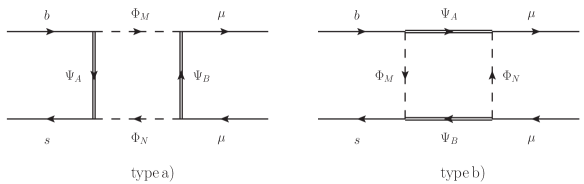
Figure 1: Box diagrams contributing to $b\to s\mu^{+}\mu^{-}$ transitions. The diagram on the left is generated in models in which the fermions couples only to SM quarks or only to SM leptons, which corresponds to type $a)$. The diagram on the right refers to models with scalars connecting $b$ to $s$ and $\mu$ to $\mu$, i.e. type $b)$.

In this section we define our generic setup and calculate completely general 1-loop expressions for contributions to $b\to s$ processes and the anomalous magnetic moment of the muon.

As outlined in the introduction, in the spirit of Refs. Gripaios:2015gra ; Arnan:2016cpy we add to the SM particle content a NP sector with vector-like fermions $\Psi_{A}$ and new scalars $\Phi_{M}$ such that $b\to s\mu^{+}\mu^{-}$ transitions can be generated via box diagrams, as depicted in Fig. 1. In this respect, we generalize the previous analysis of Ref. Arnan:2016cpy by including in addition couplings of new particles to $SU(2)$ singlet SM fermions. Moreover, we do not impose limitations on the number of fields added to the SM and allow for couplings of the new sector to the SM Higgs.

In order to generate box diagrams as the ones shown in Fig. 1 it is necessary that either the scalars $\Phi_{M,N}$ or the fermions $\Psi_{A,B}$ couple both to quarks and leptons, corresponding to case $a)$ and $b)$, respectively. This means that in diagrams of type $a)$ the amplitudes (before using any Fierz identities) have the structure $(\bar{s}\Gamma b)(\bar{\mu}\Gamma\mu)$, while in type $b)$ amplitudes of the form $(\bar{\mu}\Gamma b)(\bar{s}\Gamma\mu)$ are generated. Here, $\Gamma$ denotes an arbitrary Dirac structure. Since semi-leptonic operators are commonly given in the form $(\bar{s}\Gamma b)(\bar{\mu}\Gamma\mu)$, Fierz identities must be used in case $b)$ in order to transform the expressions to this standard basis. We give the relevant Fierz identities in Appendix A.

The Yukawa-like couplings of new scalars $\Phi_{M}$ and fermions $\Psi_{A}$ to bottom/strange quarks and muons can be parameterized completely generically (below the EWSB scale) by the Lagrangian

$$\mathcal{L}_{\rm int}= \bigg{[} \bar{\Psi}_{A}\left(L_{AM}^{b}{P_{L}}{b}+L_{AM}^{s}{P_{L}}{s}+L_{AM}^{\mu}{P_{L}}\mu\right){\Phi_{M}}$$ (1)

$$+\bar{\Psi}_{A}\left({R_{AM}^{b}{P_{R}}{b}+R_{AM}^{s}{P_{R}}{s}+R_{AM}^{\mu}{P_{R}}\mu}\right){\Phi_{M}}\bigg{]}+\mathrm{h.c.}\,.$$

Here $\Psi_{A}$ and $\Phi_{M}$ have to be understood as generic lists containing in principle an arbitrary number of fields, meaning that $A$ and $M$ also include implicitly $SU(2)$ and color indices. Therefore, the couplings $L_{AM}^{s,b}$ and $R_{AM}^{s,b}$ are generic matrices in ($A$-$M$) space with the restriction that $U(1)_{\rm EM}$ and $SU(3)$ are respected.

This Lagrangian will not only affect $b\to s\mu^{+}\mu^{-}$ transitions but also unavoidably generate effects in $B_{s}-\bar{B}_{s}$ mixing, $b\to s\gamma$ decays, the anomalous magnetic moment of the muon $a_{\mu}$ as well as $Z$ couplings and decays to SM fermions. Furthermore, $b\to s\nu\bar{\nu}$ processes and $D_{0}-\bar{D}_{0}$ mixing can give relevant constraints once $SU(2)$ invariance at the NP scale is imposed. Therefore, all these processes have to be taken into account in a complete phenomenological analysis. In order to perform such an analysis, the Wilson coefficients of the relevant effective Hamiltonian must be known. We will calculate them in the following subsections.

2.1 $b\to s\mu^{+}\mu^{-}$ and $b\to s\gamma$ Transitions

The dimension-6 operators governing $b\to s\mu^{+}\mu^{-}$ and $b\to s\gamma$ transitions are contained in the effective Hamiltonian:

$$\mathcal{H}_{\mathrm{eff}}^{\ell\ell}=-\frac{4G_{F}}{\sqrt{2}}V_{tb}V_{ts}^{\ast}\sum\limits_{\begin{subarray}{c}i\end{subarray}}\Bigg{(}C_{i}(\mu)\mathcal{O}_{i}(\mu)+C_{i}^{\prime}(\mu)\mathcal{O}_{i}^{\prime}(\mu)\Bigg{)}+\mathrm{h.c.}\,,$$ (2)

where

$$\mathcal{O}_{7} =\frac{e}{16\pi^{2}}m_{b}\bar{s}\sigma^{\mu\nu}P_{R}bF_{\mu\nu}\,,\qquad\qquad \mathcal{O}_{8} =\frac{g_{s}}{16\pi^{2}}m_{b}\bar{s}_{\alpha}\sigma^{\mu\nu}P_{R}T^{a}_{\alpha\beta}b_{\beta}G_{\mu\nu}^{a}\,,$$

$$\mathcal{O}_{9} =\frac{\alpha_{\text{EM}}}{4\pi}(\bar{s}\gamma_{\mu}P_{L}b)(\bar{\mu}\gamma^{\mu}\mu)\,,\qquad\qquad \mathcal{O}_{10} =\frac{\alpha_{\text{EM}}}{4\pi}(\bar{s}\gamma_{\mu}P_{L}b)(\bar{\mu}\gamma^{\mu}\gamma_{5}\mu)\,,$$

$$\mathcal{O}_{S} =\frac{\alpha_{\text{EM}}}{4\pi}(\bar{s}P_{R}b)(\bar{\mu}\mu)\,,\qquad\qquad \mathcal{O}_{P} =\frac{\alpha_{\text{EM}}}{4\pi}(\bar{s}P_{R}b)(\bar{\mu}\gamma_{5}\mu)\,,$$

$$\mathcal{O}_{T} =\frac{\alpha_{\text{EM}}}{4\pi}(\bar{s}\sigma_{\mu\nu}b)(\bar{\mu}\sigma^{\mu\nu}P_{R}\mu)\,,$$ (3)

with $e$ being the electron charge, $\alpha_{\text{EM}}$ the fine structure constant and $g_{s}$ the $SU(3)$ gauge coupling. The primed operators are obtained by interchanging $L$ and $R$. NP contributions from box diagrams will generate effects in $C^{(\prime)}_{9,10}$, $C^{(\prime)}_{S,P}$ and $O^{(\prime)}_{T}$, while on-shell photon (gluon) penguins generate $C^{(\prime)}_{7(8)}$ and $C^{(\prime)}_{9}$, and $Z$-penguins $C^{(\prime)}_{9,10}$.

$SU(3)$	$b\to s\ell\bar{\ell}$  type $a)$				$b\to s\ell\bar{\ell}$  type $b)$				$\chi$
	$\Psi_{A}$	$\Psi_{B}$	$\Phi_{M}$	$\Phi_{N}$	$\Psi_{A}$	$\Psi_{B}$	$\Phi_{M}$	$\Phi_{N}$
I	3	1	1	1	1	1	$\bar{3}$	1	1
II	1	$\bar{3}$	$\bar{3}$	$\bar{3}$	3	3	1	3	1
III	3	8	8	8	8	8	$\bar{3}$	8	4/3
IV	8	$\bar{3}$	$\bar{3}$	$\bar{3}$	3	3	8	3	4/3
V	$\bar{3}$	3	3	3	$\bar{3}$	$\bar{3}$	3	$\bar{3}$	2

Table 1: Table of the possible $SU(3)$ representations that can give an effect in $b\to s\ell^{+}\ell^{-}$ or $b\to s\nu\nu$ transitions via box diagrams. $\chi$ denotes the resulting group factor appearing in Eqs. (4)-(8) which also enters in $b\to s\nu\nu$ transitions.

The box diagrams in Fig. 1, result in the following Wilson coefficients (here and in the remainder of the section, an implicit sum over all NP particles, i.e. $A,B,M,N$, is understood):

$$C_{9}^{\text{box},\,a)} = -{\cal N}\frac{\chi L^{s*}_{AN}L^{b}_{AM}}{{32\pi\alpha_{\text{EM}}m_{\Phi_{M}}^{2}}}\left[L^{\mu*}_{BM}L^{\mu}_{BN}+R^{\mu*}_{BM}R^{\mu}_{BN}\right]F(x_{AM},x_{BM},x_{NM})\,,$$

$$C_{9}^{{\text{box},\,b)}} = -{\cal N}\frac{\chi L^{s*}_{BM}L^{b}_{AM}}{{32\pi\alpha_{\text{EM}}m_{\Phi_{M}}^{2}}}\bigg{[}L^{\mu*}_{AN}L^{\mu}_{BN}F(x_{AM},x_{BM},x_{NM})$$ (4)

$$\qquad\qquad\qquad\qquad-R^{\mu*}_{AN}R^{\mu}_{BN}\frac{m_{\Psi_{A}}m_{\Psi_{B}}}{m_{\Phi_{M}}^{2}}G(x_{AM},x_{BM},x_{NM})\bigg{]}\,,$$

$$C_{10}^{{\text{box},\,a)}} = {\cal N}\frac{\chi L^{s*}_{AN}L^{b}_{AM}}{{32\pi\alpha_{\text{EM}}m_{\Phi_{M}}^{2}}}\left[L^{\mu*}_{BM}L^{\mu}_{BN}-R^{\mu*}_{BM}R^{\mu}_{BN}\right]F(x_{AM},x_{BM},x_{NM})\,,$$

$$C_{10}^{{\text{box},\,b)}} = {\cal N}\frac{\chi L^{s*}_{BM}L^{b}_{AM}}{{32\pi\alpha_{\text{EM}}m_{\Phi_{M}}^{2}}}\bigg{[}L^{\mu*}_{AN}L^{\mu}_{BN}F(x_{AM},x_{BM},x_{NM})$$ (5)

$$\qquad\qquad\qquad\quad+R^{\mu*}_{AN}R^{\mu}_{BN}\frac{m_{\Psi_{A}}m_{\Psi_{B}}}{m_{\Phi_{M}}^{2}}G(x_{AM},x_{BM},x_{NM})\bigg{]}\,,$$

$$C_{S}^{{\text{box},\,a)}} = -{\cal N}\frac{\chi L^{s*}_{AN}R^{b}_{AM}}{{16\pi\alpha_{\text{EM}}m_{\Phi_{M}}^{2}}}\left[R^{\mu*}_{BM}L^{\mu}_{BN}+L^{\mu*}_{BM}R^{\mu}_{BN}\right]\frac{m_{\Psi_{A}}m_{\Psi_{B}}}{m_{\Phi_{M}}^{2}}G(x_{AM},x_{BM},x_{NM})\,,$$

$$C_{S}^{{\text{box},\,b)}} = {\cal N}\frac{\chi L^{s*}_{BM}R^{b}_{AM}}{{16\pi\alpha_{\text{EM}}m_{\Phi_{M}}^{2}}}\bigg{[}R^{\mu*}_{AN}L^{\mu}_{BN}F(x_{AM},x_{BM},x_{NM})$$ (6)

$$\qquad\qquad\qquad\quad+L^{\mu*}_{AN}R^{\mu}_{BN}\frac{m_{\Psi_{A}}m_{\Psi_{B}}}{2m_{\Phi_{M}}^{2}}G(x_{AM},x_{BM},x_{NM})\bigg{]}\,,$$

$$C_{P}^{{\text{box},\,a)}} = {\cal N}\frac{\chi L^{s*}_{AN}R^{b}_{AM}}{{16\pi\alpha_{\text{EM}}m_{\Phi_{M}}^{2}}}\left[R^{\mu*}_{BM}L^{\mu}_{BN}-L^{\mu*}_{BM}R^{\mu}_{BN}\right]\frac{m_{\Psi_{A}}m_{\Psi_{B}}}{m_{\Phi_{M}}^{2}}G(x_{AM},x_{BM},x_{NM})\,,$$

$$C_{P}^{{\text{box},\,b)}} = -{\cal N}\frac{\chi L^{s*}_{BM}R^{b}_{AM}}{{16\pi\alpha_{\text{EM}}m_{\Phi_{M}}^{2}}}\bigg{[}R^{\mu*}_{AN}L^{\mu}_{BN}F(x_{AM},x_{BM},x_{NM})$$ (7)

$$\qquad\qquad\qquad\quad-L^{\mu*}_{AN}R^{\mu}_{BN}\frac{m_{\Psi_{A}}m_{\Psi_{B}}}{2m_{\Phi_{M}}^{2}}G(x_{AM},x_{BM},x_{NM})\bigg{]}\,,$$

$$C_{T}^{\text{box},\,b)} = -{\cal N}\frac{\chi L^{s*}_{BM}R^{b}_{AM}L^{\mu*}_{AN}R^{\mu}_{BN}}{{16\pi\alpha_{\text{EM}}m_{\Phi_{M}}^{2}}}\frac{m_{\Psi_{A}}m_{\Psi_{B}}}{m_{\Phi_{M}}^{2}}G(x_{AM},x_{BM},x_{NM})\,,$$ (8)

$SU(3)$	$\Psi_{A}$	$\Phi_{M}$	$\chi_{\gamma}$	$\chi_{g}$	$\tilde{\chi}_{g}$
I	3	1	1	1	0
II	1	$\bar{3}$	1	0	1
III	3	8	4/3	-1/6	3/2
IV	8	$\bar{3}$	4/3	3/2	-1/6
V	$\bar{3}$	3	2	-1	1

Table 2: Table of the different $SU(3)$ representations that can give non-zero effects via photon- and gluon-penguin diagrams to $b\to s\mu^{+}\mu^{-}$ transitions. $\chi_{\gamma}$ denotes the resulting group factor for the former contribution, while $\chi_{g}$ and $\tilde{\chi}_{g}$ represent the resulting group factors for the latter.

$$C_{9,S,T}^{\prime\text{box}\,}=C_{9,S,T}^{\text{box}\,}\left(L\leftrightarrow R\right)\,,\qquad\qquad C_{10,P}^{\prime\text{box}\,}=-C_{10,P}^{\text{box}\,}\left(L\leftrightarrow R\right)\,,$$ (9)

where we have defined

$$x_{AM}\equiv(m_{\Psi_{A}}/m_{\Phi_{M}})^{2},\qquad x_{BM}\equiv(m_{\Psi_{B}}/m_{\Phi_{M}})^{2},\qquad x_{NM}\equiv(m_{\Phi_{N}}/m_{\Phi_{M}})^{2}\,,$$ (10)

and

$${\cal N}^{-1}=\dfrac{4G_{F}}{\sqrt{2}}V_{tb}V_{ts}^{*}\,.$$ (11)

In the equations above, the labels $A$, $B$, $M$ and $N$ denote the particle (in case of several representations) and also include $SU(2)$ components, while the sum over $SU(3)$ indices is encoded in the group factors $\chi$. The dimensionless loop functions $F$ and $G$ are defined in Appendix B.

Such box contributions are only possible if both color and electric charge are conserved. While the Wilson coefficients of $b\to s\ell\ell$ operators are insensitive to the electric charge of the particle in the box, concerning $SU(3)$, the different possible representations of the new particles lead to distinct group factors $\chi$ in Eqs. (4)-(8). These group factors are different for type $a)$ and $b)$ and are given for all the possible representations in Tab. 1. Furthermore, crossed box diagrams can be constructed in some particular cases. We give the corresponding expressions for such in Appendix C.1 for the real scalar (or Majorana fermion) case and in Appendix D for the crossed diagrams arising with complex scalars.

On-shell photon penguins diagrams in Fig. 2 affect $C_{7}^{(\prime)}$ while off-shell ones enter $C_{9}^{\gamma(\prime)}$:

$$C_{7} = {\cal N}\dfrac{\chi_{\gamma}L^{b}_{AM}}{2m_{\Phi_{M}}^{2}}\,\left[L^{s*}_{AM}\left(Q_{\Phi_{M}}\widetilde{F}_{7}\left(x_{AM}\right)-Q_{\Psi_{A}}F_{7}\left(x_{AM}\right)\right)\right.$$ (12)

$$\qquad\qquad\quad\left.+R^{s*}_{AM}\dfrac{4m_{\Psi_{A}}}{m_{b}}\left(Q_{\Phi_{M}}\widetilde{G}_{7}\left(x_{AM}\right)-Q_{\Psi_{A}}G_{7}\left(x_{AM}\right)\right)\right]\,,$$

$$C_{9}^{\gamma} = {\cal N}\frac{\chi_{\gamma}L^{s*}_{AM}L^{b}_{AM}}{{2m_{\Phi_{M}}^{2}}}\left[{{Q_{\Phi_{M}}}{\widetilde{F}_{9}}\!\left(x_{AM}\right)-Q_{\Psi_{A}}{\widetilde{G}_{9}}\!\left(x_{AM}\right)}\right]\,,$$ (13)

$$C_{7}^{\prime} = C_{7}\left(L\leftrightarrow R\right)\,,\qquad\qquad C_{9}^{\gamma\prime}=C_{9}^{\gamma}\left(L\leftrightarrow R\right)\,,$$ (14)

where $m_{b}$ is the $b$ quark mass. $Q_{\Phi_{M}}$ and $Q_{\Psi_{A}}$ are the electric charges of the NP fields ${\Phi_{M}}$ and ${\Psi_{A}}$, respectively. The conservation of electric charge imposes that $Q_{\Phi_{M}}+Q_{\Psi_{A}}=Q_{d}\equiv-1/3$. The color factors $\chi_{\gamma}$, which depend on the $SU(3)$ representations of the new particles in the loop, are given in Tab. 2. The loop functions are defined in Appendix B. Note that the terms proportional to ${\widetilde{F}_{7}}$, ${\widetilde{G}_{7}}$ and ${\widetilde{F}_{9}}$ in Eqs. (12)-(14) stem from the diagram where the photon couples to the scalar $\Phi_{M}$, while the terms proportional to $F_{7}$, $G_{7}$ and ${\widetilde{G}}_{9}$ stem from the diagram where the photon couples to the fermion $\Psi_{A}$.

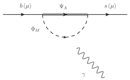
Figure 2: Photon-penguin diagrams contributing to $b\to s\gamma$ transitions and $a_{\mu}$.

Similarly, the gluon-penguin generates

$$C_{8} = {\cal N}\dfrac{L^{b}_{AM}}{2m_{\Phi_{M}}^{2}}\,\left[L^{s*}_{AM}\left(\chi_{g}\widetilde{F}_{7}\left(x_{AM}\right)-\tilde{\chi}_{g}F_{7}\left(x_{AM}\right)\right)\right.$$ (15)

$$\qquad\qquad\quad\left.+R^{s*}_{AM}\dfrac{4m_{\Psi_{A}}}{m_{b}}\left(\chi_{g}\widetilde{G}_{7}\left(x_{AM}\right)-\tilde{\chi}_{g}G_{7}\left(x_{AM}\right)\right)\right]\,,$$

$$C_{8}^{\prime} = C_{8}\left(L\leftrightarrow R\right)\,,$$ (16)

where the color factors $\chi_{g}$ and $\tilde{\chi}_{g}$ for the different possible $SU(3)$ representations are given in Tab. 2.

The contribution of $Z$-penguins to $C_{9,10}^{(\prime)}$ is given in Sec. 2.6 together with a discussion of Z decays.

2.2 $b\to s\nu\bar{\nu}$

As stated at the beginning of this section, $b\to s\nu_{\mu}\bar{\nu}_{\mu}$ processes have to be taken into account once $SU(2)$ invariance at the NP scale is imposed. This implies that, in the generic description in Eq. (1), one has to replace the left-handed muon fields with neutrinos. The box diagrams generating $b\to s\nu_{\mu}\bar{\nu}_{\mu}$ are therefore obtained from Fig. 1 by replacing muons with neutrinos.

The effective Hamiltonian describing this process reads (following the conventions of Ref. Buras:2014fpa )

$${{\cal H}_{\rm eff}^{\nu_{\mu}}}=-\frac{{4{G_{F}}}}{{\sqrt{2}}}{V_{tb}}V_{ts}^{*}\;\left(C_{L}{\mathcal{O}_{L}}+C_{R}{\mathcal{O}_{R}}\right)+\text{h.c.}\,,$$ (17)

where

$$\mathcal{O}_{L(R)}=\frac{\alpha_{\mathrm{EM}}}{{4\pi}}[\bar{s}{\gamma^{\mu}}{P_{L(R)}}b][{{\bar{\nu}}_{\mu}}{\gamma_{\mu}}\left({1-{\gamma^{5}}}\right){\nu_{\mu}}]\,.$$ (18)

The resulting WCs are:

$$C_{L}^{a)} = -{\cal N}\frac{\chi L^{s*}_{AN}L^{b}_{AM}L^{\mu*}_{BM}L^{\mu}_{BN}}{{32\pi\alpha_{\text{EM}}m_{\Phi_{M}}^{2}}}F(x_{AM},x_{BM},x_{NM})\,,$$

$$C_{L}^{b)} = {\cal N}\frac{\chi L^{s*}_{BN}L^{b}_{AM}L^{\mu*}_{AN}L^{\mu}_{BN}}{{32\pi\alpha_{\text{EM}}m_{\Phi_{M}}^{2}}}F(x_{AM},x_{BM},x_{NM})\,,$$ (19)

$$C_{R}^{a)} = -{\cal N}\frac{\chi R^{s*}_{AN}R^{b}_{AM}L^{\mu*}_{BM}L^{\mu}_{BN}}{{32\pi\alpha_{\text{EM}}m_{\Phi_{M}}^{2}}}F(x_{AM},x_{BM},x_{NM})\,,$$

$$C_{R}^{b)} = -{\cal N}\frac{\chi R^{s*}_{BN}R^{b}_{AM}L^{\mu*}_{AN}L^{\mu}_{BN}}{{32\pi\alpha_{\text{EM}}m_{\Phi_{M}}^{2}}}\frac{m_{\Psi_{A}}m_{\Psi_{B}}}{m_{\Phi_{M}}^{2}}G(x_{AM},x_{BM},x_{NM})\,,$$ (20)

where the normalization factor $\cal N$ has been introduced in Eq. (11), and the loop functions $F(x,y,z)$ and $G(x,y,z)$ are defined in Appendix B. The colour factor $\chi$ is the same as for $b\to s\mu^{+}\mu^{-}$ transitions and is given in Tab. 1 for the different representations.

2.3 $\Delta B=\Delta S=2$ Processes

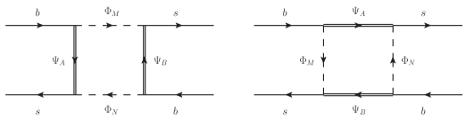
Figure 3: Box diagrams contributing to $B_{s}-{\bar{B}}_{s}$ mixing. Both diagrams arise independently of the nature of the mediator involved in $b\to s\mu^{+}\mu^{-}$ transitions.

The presence of $L_{AM}^{b,s}$ and $R_{AM}^{b,s}$ implies NP contributions to the $B_{s}-\bar{B}_{s}$ mixing which, using the conventions of Refs. Gabbiani:1996hi ; Bagger:1997gg , is governed by

$$\mathcal{H}_{\rm eff}^{B_{s}\bar{B}_{s}}=C_{i}\sum_{i=1}^{5}\mathcal{O}_{i}+\tilde{C}_{i}\sum_{i=1}^{3}\widetilde{\mathcal{O}}_{i}+\text{h.c.}\,,$$ (21)

with

$$\begin{split}\mathcal{O}_{1}&=({\bar{s}}_{\alpha}\gamma^{\mu}P_{L}b_{\alpha})\,({\bar{s}}_{\beta}\gamma^{\mu}P_{L}b_{\beta})\,,\qquad\widetilde{\mathcal{O}}_{1}=({\bar{s}}_{\alpha}\gamma^{\mu}P_{R}b_{\alpha})\,({\bar{s}}_{\beta}\gamma^{\mu}P_{R}b_{\beta})\,,\\ \mathcal{O}_{2}&=({\bar{s}}_{\alpha}P_{L}b_{\alpha})\,({\bar{s}}_{\beta}P_{L}b_{\beta})\,,\qquad\qquad\widetilde{\mathcal{O}}_{2}=({\bar{s}}_{\alpha}P_{R}b_{\alpha})\,({\bar{s}}_{\beta}P_{R}b_{\beta})\,,\\ \mathcal{O}_{3}&=({\bar{s}}_{\alpha}P_{L}b_{\beta})\,({\bar{s}}_{\beta}P_{L}b_{\alpha})\,,\qquad\qquad\widetilde{\mathcal{O}}_{3}=({\bar{s}}_{\alpha}P_{R}b_{\beta})\,({\bar{s}}_{\beta}P_{R}b_{\alpha})\,,\\ \mathcal{O}_{4}&=({\bar{s}}_{\alpha}P_{L}b_{\alpha})\,({\bar{s}}_{\beta}P_{R}b_{\beta})\,,\\ \mathcal{O}_{5}&=({\bar{s}}_{\alpha}P_{L}b_{\beta})\,({\bar{s}}_{\beta}P_{R}b_{\alpha})\,.\end{split}$$ (22)

$SU(3)$	$\Psi_{A}$	$\Psi_{B}$	$\Phi_{M}$	$\Phi_{N}$	$\chi_{BB}$	$\tilde{\chi}_{BB}$
I	3	3	1	1	1	0
II	1	1	$\bar{3}$	$\bar{3}$	0	1
III	3	3	8	8	1/36	7/12
IV	8	8	$\bar{3}$	$\bar{3}$	7/12	1/36
V	3	3	(1,8)	(8,1)	-1/6	1/2
VI	(1,8)	(8,1)	$\bar{3}$	$\bar{3}$	1/2	-1/6
VII	$\bar{3}$	$\bar{3}$	3	3	1	1

Table 3: Table of the different $SU(3)$ representations that can give a non-zero effect via box diagrams to $B_{s}-\bar{B}_{s}$ mixing. $\chi_{BB}$ and $\tilde{\chi}_{BB}$ denote the resulting group factors.

The box diagrams contributing to these above operators are shown in Fig. 3. Using the Lagrangian from Eq. (1), one obtains the following results for the coefficients:

$$C_{1} = (\chi_{BB}+\tilde{\chi}_{BB})\frac{L^{s*}_{AN}L^{b}_{AM}L^{s*}_{BM}L^{b}_{BN}}{128\pi^{2}m_{\Phi_{M}}^{2}}F\left(x_{AM},x_{BM},x_{NM}\right)\,,$$ (23)

$$C_{2} = \chi_{BB}\frac{R^{s*}_{AN}L^{b}_{AM}R^{s*}_{BM}L^{b}_{BN}}{64\pi^{2}m_{\Phi_{M}}^{2}}\frac{m_{\Psi_{A}}m_{\Psi_{B}}}{m_{\Phi_{M}}^{2}}G\left(x_{AM},x_{BM},x_{NM}\right)\,,$$ (24)

$$C_{3} = \tilde{\chi}_{BB}\frac{R^{s*}_{AN}L^{b}_{AM}R^{s*}_{BM}L^{b}_{BN}}{64\pi^{2}m_{\Phi_{M}}^{2}}\frac{m_{\Psi_{A}}m_{\Psi_{B}}}{m_{\Phi_{M}}^{2}}G\left(x_{AM},x_{BM},x_{NM}\right)\,,$$ (25)

$$C_{4} = \chi_{BB}\frac{R^{s*}_{AN}L^{b}_{AM}L^{s*}_{BM}R^{b}_{BN}}{32\pi^{2}m_{\Phi_{M}}^{2}}\frac{m_{\Psi_{A}}m_{\Psi_{B}}}{m_{\Phi_{M}}^{2}}G\left(x_{AM},x_{BM},x_{NM}\right)$$ (26)

$$-\tilde{\chi}_{BB}\frac{R^{s*}_{AN}R^{b}_{AM}L^{s*}_{BM}L^{b}_{BN}}{32\pi^{2}m_{\Phi_{M}}^{2}}F\left(x_{AM},x_{BM},x_{NM}\right)\,,$$

$$C_{5} = \tilde{\chi}_{BB}\frac{R^{s*}_{AN}L^{b}_{AM}L^{s*}_{BM}R^{b}_{BN}}{32\pi^{2}m_{\Phi_{M}}^{2}}\frac{m_{\Psi_{A}}m_{\Psi_{B}}}{m_{\Phi_{M}}^{2}}G\left(x_{AM},x_{BM},x_{NM}\right)$$ (27)

$$-\chi_{BB}\frac{R^{s*}_{AN}R^{b}_{AM}L^{s*}_{BM}L^{b}_{BN}}{32\pi^{2}m_{\Phi_{M}}^{2}}F\left(x_{AM},x_{BM},x_{NM}\right)\,,$$

$$\widetilde{C}_{1,2,3} = C_{1,2,3}\left(L\leftrightarrow R\right)\,.$$ (28)

The loop functions $F(x,y,z)$ and $G(x,y,z)$ are defined in Appendix B and the colour factors $\chi_{BB}$ and $\tilde{\chi}_{BB}$ are given in Tab. 3 for the different allowed representations. Again, in the presence of Majorana fermions or real scalars crossed diagrams can be constructed and the resulting expressions are given in Appendix C.2.

2.4 $D_{0}-\bar{D}_{0}$ Mixing

NP contributions to the $D_{0}-\bar{D}_{0}$ mixing can be obtained in complete generality (at the low scale) from Eqs. (23)-(28) by making the substitutions $s\to u$, $b\to c$, introducing couplings $L^{u,c}_{AM}$ and $R^{u,c}_{AM}$ of new scalars and fermions to up-quarks in straightforward extension of Eq. (1).

In the context a UV complete model, $SU(2)$ invariance imposes at the high scale that couplings to left-handed up-type quarks are related to the couplings to left-handed down-type quarks via CKM rotations. Therefore, working in the down-basis, the “minimal” effect generated in $D_{0}-\bar{D}_{0}$ is induced by the couplings

$$L^{u}_{AM}=V_{us}^{*}L^{s}_{AM}+V_{ub}^{*}L^{b}_{AM}\,,\qquad L^{c}_{AM}=V_{cs}^{*}L^{s}_{AM}+V_{cb}^{*}L^{b}_{AM}\,.$$ (29)

2.5 Anomalous Magnetic Moment of the Muon

$SU(3)$	$\Psi_{A}$	$\Phi_{M}$	$\chi_{a_{\mu}}$
I	1	1	1
II	(3,$\bar{3}$)	(3,$\bar{3}$)	3
III	8	8	8

Table 4: Table of the different $SU(3)$ representations that can give a non-zero effect to $a_{\mu}$. $\chi_{a_{\mu}}$ denotes the resulting group factor.

The anomalous magnetic moment of the muon ($a_{\mu}\equiv(g-2)_{\mu}/2$) and its electric dipole moments ($d_{\mu}$) we find from the diagrams in Fig. 2

$$\Delta a_{\mu} = \dfrac{\chi_{a_{\mu}}m_{\mu}^{2}}{8\pi^{2}m_{\Phi_{M}}^{2}}\,\left[\left(L^{\mu*}_{AM}L^{\mu}_{AM}+R^{\mu*}_{AM}R^{\mu}_{AM}\right)\left(Q_{\Phi_{M}}\widetilde{F}_{7}\left(x_{AM}\right)-Q_{\Psi_{A}}F_{7}\left(x_{AM}\right)\right)\right.$$

$$\qquad\qquad\quad+\left.\left(L^{\mu*}_{AM}R^{\mu}_{AM}+R^{\mu*}_{AM}L^{\mu}_{AM}\right)\dfrac{2m_{\Psi_{A}}}{m_{\mu}}\left(Q_{\Phi_{M}}\widetilde{G}_{7}\left(x_{AM}\right)-Q_{\Psi_{A}}G_{7}\left(x_{AM}\right)\right)\right]\,,$$

$$d_{\mu} = \dfrac{\chi_{a_{\mu}}m_{\Psi_{A}}}{8\pi^{2}m_{\Phi_{M}}^{2}}\,e\left(L^{\mu*}_{AM}R^{\mu}_{AM}-R^{\mu*}_{AM}L^{\mu}_{AM}\right)\left(Q_{\Phi_{M}}\widetilde{G}_{7}\left(x_{AM}\right)-Q_{\Psi_{A}}G_{7}\left(x_{AM}\right)\right)\,,$$ (31)

where $m_{\mu}$ is the muon mass, $\chi_{a_{\mu}}$ is the colour factor given in Table 4, and $Q_{\Phi_{M}}$ and $Q_{\Psi_{A}}$ are the electric charges of the NP fields ${\Phi_{M}}$ and ${\Psi_{A}}$, respectively. Analogously to photon-penguin contributions to $b\to s$ transitions, the conservation of electric charge imposes that $Q_{\Phi_{M}}+Q_{\Psi_{A}}=Q_{\mu}\equiv-1$. Finally, the loop functions $F_{7}(x)$, $\widetilde{F}_{7}(x)$, $G_{7}(x)$ and $\widetilde{G}_{7}(x)$ are defined in Appendix B.

2.6 Modified $Z$ Couplings

Here, we study the effects of our new particles on modified $Z$ couplings, i.e. on $Z\bar{\mu}\mu$, $Z\bar{b}b$, $Z\bar{s}s$ and $Z\bar{s}b$ couplings, both for off- and on-shell $Z$ bosons. We define the form-factors governing $Z\bar{f}f$ interactions as Dedes:2017zog

$$-\dfrac{g_{2}}{c_{W}}\bar{f^{\prime}}\gamma^{\mu}\Big{[}g^{f^{\prime}f}_{L}(q^{2})\,P_{L}+g^{f^{\prime}f}_{R}(q^{2})\,P_{R}\Big{]}f\,Z_{\mu}+\text{h.c.}\,,$$ (32)

where $f=\{b,s,\,\mu\}$, $g_{2}$ is the $SU(2)$ gauge coupling, $\theta_{W}$ the Weinberg angle and $q$ is the $Z$ momentum. Moreover,

$$g^{f^{\prime}f}_{L(R)}(q^{2})=g_{f_{L}}^{\mathrm{SM}}\delta_{f^{\prime}f}+\Delta g^{f^{\prime}f}_{L(R)}(q^{2})$$ (33)

with $g_{f_{L}}^{\mathrm{SM}}=(T_{3}^{f}-Q_{f}s^{2}_{W})$ and $g_{f_{R}}^{\mathrm{SM}}=-Q_{f}s^{2}_{W}$ being the $Z$ couplings to SM fermions at tree-level. The relevant Feynman diagrams are shown in Fig. 4. We write the coupling of the $Z$ boson to the new scalars and fermions as

$$\mathcal{L}^{Z}=-\dfrac{g_{2}}{c_{W}}Z_{\mu}\left(\bar{\Psi}_{A}\gamma^{\mu}\Big{[}g^{\Psi,L}_{AB}\,P_{L}+g^{\Psi,R}_{AB}\,P_{R}\Big{]}\Psi_{B}+g^{\Phi}_{MN}\,\Phi_{M}^{\dagger}\,i\overset{\leftrightarrow}{\partial^{\mu}}\,\Phi_{N}\,\right)+\mathrm{h.c.}\,,$$ (34)

where we have introduced the notation $a\overset{\leftrightarrow}{\partial^{\mu}}b=a({\partial^{\mu}}b)-({\partial^{\mu}}a)b$, and with generic couplings $g^{\Psi,L,R}_{AB}$ and $g^{\Phi}_{MN}$ which can only be determined in a UV complete model in which also the couplings of the new particles to the SM Higgs are known. Using the generic Lagrangian from Eq. (1), one obtains the following results for the coefficients

$$\Delta g^{f^{\prime}f}_{L}(q^{2}) = \dfrac{\chi_{Z}\,L^{f^{\prime}}_{BN}L^{f*}_{AM}}{{32\pi^{2}}}$$ (35)

$$\qquad\left[2\,g_{AB}^{\Psi,L}\delta_{MN}\dfrac{m_{\Psi_{A}}m_{\Psi_{B}}}{m_{\Phi_{M}}^{2}}G_{Z}(x_{AM},x_{BM})-g_{AB}^{\Psi,R}\delta_{MN}F_{Z}(x_{AM},x_{BM},m_{\Phi_{M}})\right.$$

$$\qquad+g_{MN}^{\Phi}\delta_{AB}H_{Z}(x_{AM},x_{AN},m_{\Psi_{A}})-\dfrac{1}{2}(g_{f_{L}}^{SM}+g_{f^{\prime}_{L}}^{SM})\delta_{AB}\delta_{MN}I_{Z}(x_{AM},m_{\Phi_{M}})$$

$$\qquad+\left.q^{2}\left(g_{AB}^{\Psi,L}\delta_{MN}\dfrac{m_{\Psi_{A}}m_{\Psi_{B}}}{m_{\Phi_{M}}^{4}}\widetilde{G}_{Z}(x_{AM},x_{BM})-\dfrac{2}{3}\dfrac{g_{AB}^{\Psi,R}\delta_{MN}}{m_{\Phi_{M}}^{2}}\widetilde{F}_{Z}(x_{AM},x_{BM})\right.\right.$$

$$\qquad\left.\left.\hskip 42.67912pt-\dfrac{1}{3}\dfrac{g_{MN}^{\Phi}\delta_{AB}}{m^{2}_{\Psi_{A}}}\widetilde{H}_{Z}(x_{AM},x_{AN})\right.\Big{)}\right.\Big{]}\,,$$

$$\Delta g^{f^{\prime}f}_{R}(q^{2}) = \Delta g^{f^{\prime}f}_{L}(q^{2})\left(L\leftrightarrow R\right)\,,$$ (36)

where the loop functions are defined in Appendix B, and the colour factor $\chi_{Z}=\chi_{\gamma}$ for $f,f^{\prime}=b,s$ (see Table 2) and $\chi_{Z}=\chi_{a_{\mu}}$ (see Table 4) for $f=\mu$. Here we have set the masses and momenta of the external fermions to 0 and expanded up to first order in $q^{2}$ over the NP scale. If one is considering data from $Z$ decays, Eq. (35) has to be evaluated to $q^{2}=m_{Z}^{2}$ while for processes with an off-shell $Z$ (like $b\to s\ell^{+}\ell^{-}$) one has to set $q^{2}=0$.

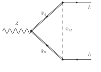
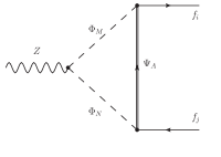
Figure 4: Feynman diagrams modifying the $Z\bar{f_{i}}f_{j}$ vertex with $f_{i}=s,\,b,\,\mu$.

Note that in the absence of EW symmetry breaking in the NP sector, the contribution of the self-energies cancel the one of the genuine vertex correction and Eq. (35) vanishes for $q^{2}=0$. Therefore, as noted above, $g^{\Psi,L}_{AB}$, $g^{\Psi,R}_{AB}$ and $g^{\Phi}_{MN}$ are only meaningful after EWSB and it is not possible to relate them purely to $SU(2)\times U(1)$ quantum numbers. In a specific UV model with a known pattern of EWSB, rotation matrices can be used to relate the couplings before and after the breaking. Consequently, the cancellation of UV divergences (present in some of the loop functions in Eq. (35)) is only manifest after summation over $SU(2)$ indices, due to a GIM-like cancellation originating from the unitarity of the rotation matrices. We will give a concrete example of this in Sec. 4.

The form-factors in Eq. (32) includes $Z\bar{s}b$ couplings generating contributions to $C_{9,{10}}^{(\prime)}$

$$C_{9}^{(\prime)\,Z} = \mathcal{N}\dfrac{\pi g^{2}}{\alpha_{\rm EM}c^{2}_{W}m_{Z}^{2}}g^{sb}_{{L(R)}}(q^{2}=0)\left(1-4s_{W}^{2}\right)\,,$$ (37)

$$C_{10}^{(\prime)\,Z} = -\mathcal{N}\dfrac{\pi g^{2}}{\alpha_{\rm EM}c^{2}_{W}m_{Z}^{2}}g^{sb}_{{L(R)}}(q^{2}=0)\,.$$ (38)

Note that these contributions are lepton flavour universal and therefore cannot account for $R_{K}$ and $R_{K^{*}}$. However, a mixture of lepton flavour universal and violating contributions is phenomenologically interesting Alguero:2018nvb , especially in the light of the recant Belle and LHCb measurements Alguero:2019ptt ; Datta:2019zca . In a similar fashion, $Z\bar{s}b$ couplings will also generate the following contributions to $b\to s\nu\bar{\nu}$ contained in $C_{L(R)}$

$$C_{L(R)}^{\,Z} = -\mathcal{N}\dfrac{\pi g^{2}}{\alpha_{\rm EM}c^{2}_{W}m_{Z}^{2}}g^{sb}_{L{(R)}}(q^{2}=0)\,.$$ (39)

Finally, if $SU(2)$ invariance at the NP scale is imposed, the new scalars and fermions couple also the neutrinos. Hence, contributions to $Z\to\nu\bar{\nu}$ and $W\to\mu\bar{\nu}$ will arise as well. Concerning $Z\to\nu\bar{\nu}$, $g_{\nu_{L}}(q^{2}=m_{Z}^{2})$ can be straightforwardly extracted from Eq. (35) by appropriate replacements and the same is true concerning $W\mu\bar{\nu}$ couplings.

3 Experimental Constraints on Wilson Coefficients

In this section we review the experimental situation and the resulting constraints on the Wilson coefficients calculated in the previous section.

3.1 $b\to s$ Transitions

The semileptonic operators $\mathcal{O}_{9,10}^{(\prime)}$, $\mathcal{O}_{S,P}^{(\prime)}$ and $\mathcal{O}_{T}^{(\prime)}$, together with magnetic operators $\mathcal{O}_{7}^{(\prime)}$, contribute to a plethora of $b\to s\ell^{+}\ell^{-}$ observables. The corresponding measurements include total branching ratios of $B_{s}\to\ell^{+}\ell^{-}$ Amhis:2016xyh , of the exclusive decays $B\to K^{*}\gamma$ Amhis:2016xyh , $B\to\phi\gamma$ Aaij:2012ita , the inclusive decay $B\to X_{s}\gamma$ Amhis:2016xyh , the angular analyses of $B\to K^{(*)}\ell^{+}\ell^{-}$ Aaij:2015oid ; Aaij:2015dea ; Aaij:2016flj ; Wehle:2016yoi ; Aaboud:2018krd ; Khachatryan:2015isa ; Sirunyan:2017dhj (proposed in Refs. Altmannshofer:2008dz ; Matias:2012xw ; Descotes-Genon:2013vna ) and $B_{s}\to\phi\,\ell^{+}\ell^{-}$ Aaij:2015esa , and also the ratios $R_{K}$ Aaij:2019wad and $R_{K^{*}}$ Aaij:2017vbb ; Abdesselam:2019wac measuring lepton flavour universality violation.

First of all, the contributions of scalar operators are helicity-enhanced in the $B_{s}\to\mu^{+}\mu^{-}$ branching ratio with respect to the $O_{10}$ contribution of the SM. This results in the bound Beneke:2017vpq

$$\dfrac{{{\mathcal{B}}^{\rm exp}}(B_{s}\to\mu^{+}\mu^{-})}{{\mathcal{B}^{\rm SM}}(B_{s}\to\mu^{+}\mu^{-})}-1 = \left|1+\dfrac{C_{10}-C_{10}^{\prime}}{C_{10}^{\text{SM}}}+\dfrac{m_{B_{s}}^{2}}{2m_{\mu}(m_{b}+m_{s})}\dfrac{C_{P}-C_{P}^{\prime}}{C_{10}^{\text{SM}}}\right|^{2}$$ (40)

$$+\dfrac{m_{B_{s}}^{2}(m_{B_{s}}^{2}-4m_{\mu}^{2})}{4m_{\mu}^{2}(m_{b}+m_{s})^{2}}\left|\dfrac{C_{S}-C_{S}^{\prime}}{C_{10}^{\text{SM}}}\right|^{2}-1=-0.13\pm 0.20\,,\quad$$

which excludes sizable contributions to scalar operators (unless there is a purely scalar quark current) and leads to

$$|C_{S,P}^{(\prime)}|\lesssim 0.03\,\quad(2\,\sigma)\,,$$ (41)

from the updated one-parameter fit of Ref. Altmannshofer:2017wqy . Therefore, we neglect the effects of scalar operators in semi-leptonic $B$ since they anyway cannot explain the corresponding anomalies.

Moreover, the inclusive $b\to s\gamma$ decay strongly constrains the magnetic operators. From Misiak:2017woa ; Misiak:2015xwa , in the limit of vanishing $C_{7,8}^{\prime}$, we have

$$\dfrac{{{\mathcal{B}}^{\rm exp}}(b\to s\gamma)}{{\mathcal{B}^{\rm SM}}(b\to s\gamma)}-1=-2.87\,\left[C_{7}+0.19\,C_{8}\right]=(-0.7\pm 8.2)\times 10^{-2}\,,$$ (42)

leading to

$$|C_{7}+0.19\,C_{8}|\lesssim 0.06\,\quad(2\,\sigma)\,.$$ (43)

Here, we used $C_{7,8}$ at a matching scale of 1 TeV as input. Again, these constraints are so stringent that the effect of $C_{7,8}$ on the flavour anomalies can be mostly neglected.

On the other hand, vector operators can explain the $b\to s\ell^{+}\ell^{-}$ anomalies. We therefore refer to global fits to constrain $C_{9,10}^{(\prime)}$, where all the relevant observables have been taken into account Capdevila:2017bsm ; Altmannshofer:2017yso ; DAmico:2017mtc ; Hiller:2017bzc ; Geng:2017svp ; Ciuchini:2017mik ; Alok:2017sui ; Hurth:2017hxg . The results of the most recent fits find at the $2\,\sigma$ level

$$\begin{aligned} -1.48&\leq C_{9}\leq-0.71\,,\qquad-0.12\leq C_{10}\leq 0.61\,,\\ -0.56&\leq C_{9}^{\prime}\leq 1.14\,,\qquad\quad-0.57\leq C_{10}^{\prime}\leq 0.34\,,\qquad\end{aligned}$$

according to Ref. Alguero:2019ptt (which is compatible with Refs. Alok:2019ufo ; Ciuchini:2019usw ; Aebischer:2019mlg ; Kowalska:2019ley ).

As explained in Sec. 2.2, $SU(2)$ invariance implies the presence of contributions to $B\to K^{(*)}\nu\bar{\nu}$ decays as well. Since there is no experimental way to distinguish different neutrino flavours in these decays, one measures the total branching ratio which we normalize to its SM prediction Buras:2014fpa :

$$R_{K^{(*)}}^{\nu\bar{\nu}}=\frac{{\mathcal{B}}^{\rm exp}(B\to K^{(*)}\nu\bar{\nu})}{{\mathcal{B}}^{\rm SM}(B\to K^{(*)}\nu\bar{\nu})}=\frac{2(C_{L}^{\rm SM})^{2}+(C_{L}^{\rm SM}+C_{L})^{2}-\kappa\ (C_{L}^{\rm SM}+C_{L})C_{R}+C_{R}^{2}}{3(C_{L}^{\rm SM})^{2}}\,.$$ (44)

In the case of a $K$ in the final state one has $\kappa\equiv-2$, while for the $K^{*}$ one gets $\kappa=1.34(4)$ Buras:2014fpa . The current experimental limits at $90\%$ C.L. are Grygier:2017tzo

$$R_{K}^{\nu\bar{\nu}}<3.9\,,\qquad\qquad R_{K^{*}}^{\nu\bar{\nu}}<2.7\,.$$ (45)

3.2 Neutral Meson Mixing

The experimental constraint on the Wilson coefficients in Eqs. (23)-(28) comes from the mass difference $\Delta M_{s}$ of neutral $B_{s}$ mesons, see e.g. Ref. Gabbiani:1996hi (in the case of real Wilson coefficients). To compare our results with experiments we use

$$\!\!\!\!\frac{\Delta M_{s}^{\rm exp}}{\Delta M_{s}^{\rm SM}} = \left|1+\sum_{i,j=1}^{3}R_{i}(\mu_{b})\frac{\eta_{ij}(\mu_{b},\mu_{H})}{C^{\rm SM}_{1}(\mu_{b})}\left(C_{j}+\widetilde{C}_{j}\right)+\sum_{i,j=4}^{5}R_{i}(\mu_{b})\frac{\eta_{ij}(\mu_{b},\mu_{H})}{C^{\rm SM}_{1}(\mu_{b})}C_{j}\right|$$ (46)

$$= \left|1+\dfrac{0.8\,(C_{1}+\widetilde{C}_{1})-1.9\,(C_{2}+\widetilde{C}_{2})+0.5\,(C_{3}+\widetilde{C}_{3})+5.2\,C_{4}+1.9\,C_{5}}{C^{\rm SM}_{1}(\mu_{b})}\right|\,,\$$

where $R_{i}(\mu_{b})$ is related to the matrix element of the operators $Q_{i}$ in Eq. (22) at the scale $\mu_{b}$ by the relation

$$R_{i}(\mu_{b})=\frac{\langle\bar{B}_{s}|Q_{i}(\mu_{b})|B_{s}\rangle}{\langle\bar{B}_{s}|Q_{1}(\mu_{b})|B_{s}\rangle}\,.$$ (47)

The coefficients $C_{i}$ and $\widetilde{C}_{i}$ are the ones in Eqs. (23)-(28), computed at the NP scale $\mu_{H}$. The matrix in operator space $\eta_{ij}(\mu_{b},\mu_{H})$ encodes the QCD evolution from the high scale $\mu_{H}$ to $\mu_{b}$, which we calculated numerically for a reference scale $\mu_{H}=1$ TeV Becirevic:2001jj . The matrix elements in Eqs. (46)-(47) have been computed by a $N_{f}=2+1$ lattice simulation Bazavov:2016nty , which found values consistent with the $N_{f}=2$ calculation Carrasco:2013zta and recent sum rules results King:2019lal . It is worth mentioning that FLAG-2019 Aoki:2019cca only provides a lattice average for $\langle\bar{B}_{s}|Q_{1}(\mu_{b})|B_{s}\rangle$, which is however dominated by the $N_{f}=2+1$ results from Ref. Bazavov:2016nty . Therefore, we decided to employ the results from Ref. Bazavov:2016nty in Eqs. (46)-(47). The SM value for the Wilson coefficient is $C^{\rm SM}_{1}(\mu_{b})=\dfrac{G_{F}^{2}M_{W}^{2}}{4\pi^{2}}\lambda_{t}^{2}\eta_{11}(\mu_{b},m_{t})S_{0}(x_{t})\simeq 7.2\times 10^{-11}\text{ GeV}^{-2}$.

The experimental constraint therefore reads Tanabashi:2018oca

$$R_{\Delta M_{s}}=\frac{\Delta M_{s}^{\rm exp}}{\Delta M_{s}^{\rm SM}}-1=-0.09\pm 0.08\,,$$ (48)

computed with the values from Ref. Bazavov:2016nty for $\langle\bar{B}_{s}|Q_{1}(\mu_{b})|B_{s}\rangle$. This value shows a slight tension with the SM as first outlined in Refs. DiLuzio:2018wch ; DiLuzio:2017fdq . The tension would be reduced if one considered the results for the matrix element from Ref. King:2019lal : however, in this case one should rely on a separate computation for the decay constant, while in Ref. Bazavov:2016nty both quantities are computed together.

Analogously to the $B_{s}$ system, $D_{0}-\bar{D}_{0}$ mixing is constrained by the mass difference of neutral $D_{0}$ mesons Tanabashi:2018oca :

$$\Delta M_{D_{0}}^{\rm exp}=(0.63^{+0.27}_{-0.29})\times 10^{-11}{\rm MeV}\,.$$ (49)

Unfortunately, a precise SM prediction is still lacking in this sector but one can constrain the NP contribution by assuming that not more than the total mass difference is generated by it.

3.3 Anomalous Magnetic Moment of the Muon

From the experimental side, this quantity has been already measured quite precisely Bennett:2006fi , but further improvements by experiments at Fermilab Grange:2015fou and J-PARC Saito:2012zz (see also Gorringe:2015cma ) are expected in the future. On the theory side, the SM prediction has been improved continuously Czarnecki:1995wq ; Czarnecki:1995sz ; Jegerlehner:2009ry ; Hagiwara:2011af ; Aoyama:2012wk ; Gnendiger:2013pva ; Chakraborty:2016mwy ; Jegerlehner:2017lbd ; DellaMorte:2017dyu ; Davier:2017zfy ; Borsanyi:2017zdw ; Giusti:2018mdh ; Giusti:2019xct ; Blum:2018mom ; Keshavarzi:2018mgv ; Colangelo:2015ama ; Green:2015sra ; Gerardin:2016cqj ; Blum:2016lnc ; Colangelo:2017qdm ; Blum:2017cer ; Hoferichter:2018dmo ; Kurz:2014wya ; Colangelo:2014qya . The current tension between the two determinations accounts to

$$\Delta a_{\mu}=a_{\mu}^{exp}-a_{\mu}^{\text{SM}}\sim 270(85)\times 10^{-11}\,.$$ (50)

3.4 $Z$ Decays

The main experimental measurements of $Z$ couplings have been performed at LEP ALEPH:2005ab (at the $Z$ pole). We extract from the model independent analysis of Ref. Efrati:2015eaa the values for the NP contributions 

$$\Delta g_{\mu_{L}}(m_{Z}^{2}) =-(0.1\pm 1.1)\times 10^{-3}\,,\qquad\qquad \Delta g_{\mu_{R}}(m_{Z}^{2})= \ (0.0\pm 1.3)\times 10^{-3}\,,$$ (51)

$$\Delta g_{b_{L}}(m_{Z}^{2}) =-(0.33\pm 0.16)\times 10^{-2}\,, \Delta g_{b_{R}}(m_{Z}^{2})= \ -(2.30\pm 0.82)\times 10^{-3}\,,$$

$$\Delta g_{\nu_{L}}(m_{Z}^{2}) =(0.40\pm 0.21)\times 10^{-2}\,,$$

neglecting cancellations and correlations.

4 ${4^{\rm th}}$ Generation Model

In this section we propose a model with a vector-like 4^th generation of fermions and a new complex scalar. This will also allow us to apply and illustrate the generic findings of the previous section to a UV complete model and study the effects in $b\to s\ell^{+}\ell^{-}$ data and $a_{\mu}$.

4.1 Lagrangian

The Lagrangian for our 4^th generation model is obtained from the SM one by adding a 4^th vector-like generation Poh:2017tfo ; Raby:2017igl and a neutral scalar

$$L^{4{\rm th}} = \sum\limits_{i}\left(\Gamma^{L}_{q_{i}}\bar{\Psi}_{q}P_{L}q_{i}+\Gamma^{L}_{\ell_{i}}\bar{\Psi}_{\ell}P_{L}\ell_{i}+\Gamma^{R}_{u_{i}}\bar{\Psi}_{u}P_{R}u_{i}+\Gamma^{R}_{d_{i}}\bar{\Psi}_{d}P_{R}d_{i}+\Gamma^{R}_{e_{i}}\bar{\Psi}_{e}P_{R}e_{i}\right)\Phi+\mathrm{h.c.}$$ (52)

$$+\sum\limits_{C=L,R}\left(\lambda_{C}^{U}\bar{\Psi}_{q}P_{C}\tilde{h}\Psi_{u}+\lambda_{C}^{D}\bar{\Psi}_{q}P_{C}h\Psi_{d}+\lambda_{C}^{E}\bar{\Psi}_{\ell}P_{C}h\Psi_{e}\right)+\mathrm{h.c.}$$

$$+\sum\limits_{F=q,\ell,u,d,e}M_{F}\bar{\Psi}_{F}\Psi_{F}+\kappa\,h^{\dagger}h\,\Phi^{\dagger}\Phi+m_{\Phi}^{2}\Phi^{\dagger}\Phi\,,$$

where $i$ is a family index and $h$ the SM Higgs doublet. The charge assignments for the new vector-like fermions $\Psi=\Psi_{L}+\Psi_{R}$ with $P_{L,R}\Psi=\Psi_{L,R}$ and the new scalar $\Phi$ are

$$\begin{array}[]{*{20}{c}}{}\hfil&\vline&{SU\!\left(3\right)}&{SU\!\left(2\right)}&{U{{\left(1\right)}}}&U^{\prime}\left(1\right)\\ \hline\cr\Psi_{q}&\vline&3&2&{1/6}&Z\\ \Psi_{u}&\vline&3&1&{2/3}&Z\\ \Psi_{d}&\vline&3&1&{-1/3}&Z\\ \Psi_{\ell}&\vline&1&2&{-1/2}&Z\\ \Psi_{e}&\vline&1&1&{-1}&Z\\ \Phi&\vline&1&1&0&-Z\end{array}\,.$$ (53)

The SM fermions have the same $SU(3)\times SU(2)\times U(1)$ charge assignments of the relative NP fermion partner, and the higgs transforms as a (1, 2, 1/2). Here we assigned to the new particles also charges under a new $U(1)$ group in order to forbid mixing with the SM particles, giving a similar effect as R-parity in the MSSM. From Table 53 we see that concerning $SU(3)$ we are dealing with cases I of our generic analysis in Tables 1-4. In particular, concerning $b\to s\mu^{+}\mu^{-}$, this model would generate diagrams of type a) in Fig. 1.

After EWSB, mass matrices for the new fermions are generated

$$L^{4{\rm th}}_{\text{mass}} = {\left({\begin{array}[]{*{20}{c}}\bar{\Psi}_{q,1}\\ {\bar{\Psi}}_{u}\end{array}}\right)^{T}}{{\bf{M}}_{U}}{P_{L}}\left({\begin{array}[]{*{20}{c}}\Psi_{q,1}\\ {{\Psi_{u}}}\end{array}}\right)+{\left({\begin{array}[]{*{20}{c}}\bar{\Psi}_{q,2}\\ {\bar{\Psi}}_{d}\end{array}}\right)^{T}}{{\bf{M}}_{D}}{P_{L}}\left({\begin{array}[]{*{20}{c}}\Psi_{q,2}\\ {{\Psi_{d}}}\end{array}}\right)$$ (67)

$$+{\left({\begin{array}[]{*{20}{c}}\bar{\Psi}_{\ell,2}\\ {{{\bar{\Psi}}_{e}}}\end{array}}\right)^{T}}{{\bf{M}}_{E}}{P_{L}}\left({\begin{array}[]{*{20}{c}}\Psi_{\ell,2}\\ {{\Psi_{e}}}\end{array}}\right)+\mathrm{h.c.}\,,$$

where ${{\bf{M}}_{U,D,E}}$ are non-diagonal mass matrices

$${{\bf{M}}_{D(U)}}=\left({\begin{array}[]{*{20}{c}}{{M_{q}}}&{\sqrt{2}v\lambda_{R}^{D(U)}}\\ {\sqrt{2}v\lambda_{L}^{{D(U)}*}}&{{M_{d(u)}}}\end{array}}\right)\,,\quad{{\bf{M}}_{E}}=\left({\begin{array}[]{*{20}{c}}{{M_{\ell}}}&{\sqrt{2}v\lambda_{R}^{E}}\\ {\sqrt{2}v\lambda_{L}^{E*}}&{{M_{e}}}\end{array}}\right)\,.$$ (68)

Here the subscripts 1 and 2 denote the $SU(2)$ component of the doublet. We diagonalize these mass matrices by performing the field redefinitions

$$P_{L}{\left({\begin{array}[]{*{20}{c}}\Psi_{q,1}\\ {\Psi_{u}}\end{array}}\right)_{I}}\to W^{U_{L}}_{IJ}\Psi^{{U_{L}}}_{J}\,,\qquad P_{L}{\left({\begin{array}[]{*{20}{c}}\Psi_{q,2}\\ {\Psi_{d}}\end{array}}\right)_{I}}\to W^{D_{L}}_{IJ}\Psi^{{D_{L}}}_{J}\,,\qquad+\quad L\to R$$ (73)

$$P_{L}\Psi_{L,1}\to\Psi^{{N_{L}}}\,,\qquad P_{L}{\left({\begin{array}[]{*{20}{c}}\Psi_{\ell,2}\\ {\Psi_{e}}\end{array}}\right)_{I}}\to W^{E_{L}}_{IJ}\Psi^{{E_{L}}}_{J}\,,\qquad+\quad L\to R$$ (76)

leading to

$$(W^{{F_{L}}\dagger}{\bf{M}}_{F}W^{{F_{R}}})_{IJ}=m_{F_{I}}\ {\delta_{IJ}}\,,\qquad{\rm with}\;F=U,D,E\,.$$ (77)

Therefore, after EWSB we have the mass eigenstates $\Psi^{U_{L,R}}_{I}$, $\Psi^{D_{L,R}}_{I}$, $\Psi^{E_{L,R}}_{I}$ and $\Psi^{N_{L,R}}$, with $I=\{1,2\}$. In particular, $\Psi^{U_{L,R}}_{I}$ and $\Psi^{D_{L,R}}_{I}$ ($\Psi^{E_{L,R}}_{I}$ and $\Psi^{N_{L,R}}$) are $SU(3)$ triplets (singlets) with the same electric charges as up-type and down-type quarks (charged-leptons and neutrinos), respectively.

The rotations introduced at Eq. (73) lead to the following Lagrangian for the interactions in the broken phase

$$L_{\rm int}^{{\text{4th}}} = \left(L_{I}^{d_{i}}\bar{\Psi}_{I}^{D}P_{L}d_{i}+L_{I}^{e_{i}}\bar{\Psi}_{I}^{E}P_{L}e_{i}+R_{I}^{d_{i}}\bar{\Psi}_{I}^{D}P_{R}d_{i}+R_{I}^{e_{i}}\bar{\Psi}_{I}^{E}P_{R}e_{i}\right)\Phi$$ (78)

$$+\left(L_{I}^{u_{i}}\bar{\Psi}_{I}^{U}P_{L}u_{i}+L^{\nu_{i}}\bar{\Psi}^{N}P_{L}\nu_{i}+R_{I}^{u_{i}}\bar{\Psi}_{I}^{U}P_{R}u_{i}\right)\Phi+\mathrm{h.c.}\,$$

which resembles Eq. (1) for the special case of our 4th generation model. Thus identify

$$L_{I}^{d_{i}} = \Gamma^{L}_{q_{i}}W_{1I}^{{D_{R}}^{*}}\,,\qquad L_{I}^{e_{i}}=\Gamma^{L}_{\ell_{i}}W_{1I}^{{E_{R}}^{*}}\,,\qquad L_{I}^{u_{i}}=\Gamma^{L}_{q_{j}}V_{ij}^{*}W_{1I}^{{U_{R}}^{*}}\,,\qquad L^{\nu_{i}}=\Gamma^{L}_{\ell_{i}}\,,$$

$$R_{I}^{d_{i}} = \Gamma^{R}_{d_{i}}W_{2I}^{{D_{L}}^{*}}\,,\qquad R_{I}^{e_{i}}=\Gamma^{R}_{e_{i}}W_{2I}^{{E_{L}}^{*}}\,,\qquad R_{I}^{u_{i}}=\Gamma^{R}_{u_{i}}W_{2I}^{{U_{L}}^{*}}\,.$$ (79)

Here we worked in the down-basis for the SM quarks which means that CKM matrices $V_{ij}$ appear in vertices involving up-type quarks. The first two columns of the above Lagrangian involves couplings with down-type quarks and charged leptons and can be directly matched on the Lagrangian in Eq. (1) for the case of only one scalar, i.e. $\Phi_{M}\equiv\Phi$ and $\Psi_{A}\equiv\{\Psi_{I}^{D},\Psi_{I}^{E}\}$. The presence of $L_{I}^{u_{i}}$ ($L^{\nu_{i}}$) resembles the fact, mentioned in Sec. 2, that left-handed couplings to down-quarks (leptons) lead via $SU(2)$ to couplings to left-handed up-quarks (neutrinos). In addition couplings to right-handed up-quarks $R_{I}^{u_{i}}$ appear in our model which are however not relevant for our phenomenology.

4.2 Wilson Coefficients

With these conventions we can now easily derive the Wilson coefficients within our model which can be directly obtained from the results of Sec. 2. In order to simplify the expressions, we will assume $M_{Q}=M_{d}\equiv m_{D}$ and $M_{L}=M_{e}\equiv m_{E}$ and only take into account couplings to $b$, $s$ and $\mu$ in Eq. (52):

$$\{\Gamma_{s}^{L}\,,\Gamma_{b}^{L}\,,\Gamma_{\mu}^{L}\,,\Gamma_{s}^{R}\,,\Gamma_{b}^{R}\,,\Gamma_{\mu}^{R}\}\,,$$ (80)

Concerning $SU(2)$ breaking effects the couplings $\lambda_{L,R}^{D}$ and $\lambda_{L,R}^{E}$ related to the down and charged leptons sector, respectively, can be relevant. However, concerning $\lambda_{L,R}^{D}$ recall that from Section 3.1 that experimental data suggests very small values for $C_{S,P}$ and $C_{7,8}$. In our model this can be achieved by assuming $\lambda_{L,R}^{D}=0$. In this limit the mass matrix ${\bf M}^{D}$ in Eq. (68) is diagonal and the corresponding rotation matrices $W^{{D_{R(L)}}}$ in Eq. (77) are equal to the identity, which implies

$$C_{S,P}\propto L_{A}^{s*}R_{A}^{b}\propto W_{1A}^{{D_{R}}}W_{2A}^{{D_{L}}^{*}}=\delta_{1A}\delta_{2A}=0\,.$$ (81)

With this setup, we obtain the following non-vanishing couplings in the quark sector of the Lagrangian in Eq. (78):

$$L_{1}^{s} = \Gamma_{s}^{L}\,,\qquad L_{1}^{b}=\Gamma_{b}^{L}\,,\qquad R_{2}^{s}=\Gamma_{s}^{R}\,,\qquad R_{2}^{b}=\Gamma_{b}^{R}\,,$$

$$L_{1}^{u} = V_{us}^{*}\ \Gamma_{s}^{L}+V_{ub}^{*}\ \Gamma_{b}^{L}\,,\qquad L_{1}^{c}=V_{cs}^{*}\ \Gamma_{s}^{L}+V_{cb}^{*}\ \Gamma_{b}^{L}\,.$$ (82)

with

$$\Gamma^{L}\equiv L^{b}_{1}L_{1}^{s*}\,,\qquad\Gamma^{R}\equiv R^{b}_{2}R_{2}^{s*}\,,\qquad x_{D(E)}\equiv\dfrac{m_{D(E)}^{2}}{m_{\Phi}^{2}}\,.$$ (83)

The expressions of Wilson coefficients for $b\to s$ processes simplify to:

$\bullet$ $b\to s\mu^{+}\mu^{-}$ and $b\to s\gamma$ (see Eqs. (4)-(16))

$$C_{9}^{{\text{box}}\,} = -{\cal N}\frac{\Gamma^{L}}{{32\pi\alpha_{\text{EM}}m_{\Phi}^{2}}}\left(|\Gamma^{L}_{\mu}|^{2}+|\Gamma^{R}_{\mu}|^{2}\right)F(x_{D},x_{E})\,,$$ (84)

$$C_{10}^{{\text{box}}\,} = {\cal N}\frac{\Gamma^{L}}{{32\pi\alpha_{\text{EM}}m_{\Phi}^{2}}}\left(|\Gamma^{L}_{\mu}|^{2}-|\Gamma^{R}_{\mu}|^{2}\right)F(x_{D},x_{E})\,,$$ (85)

$$C_{9}^{\gamma} = {\cal N}\dfrac{\Gamma^{L}}{6m_{\Phi}^{2}}\widetilde{G}_{9}\left(x_{D}\right)\,,\>\>C_{7}={\cal N}\dfrac{\Gamma^{L}}{6m_{\Phi}^{2}}F_{7}\left(x_{D}\right)\,,\>\>C_{8}=\ -{\cal N}\dfrac{\Gamma^{L}}{2m_{\Phi}^{2}}F_{7}\left(x_{D}\right)\,,$$ (86)

$$C_{9}^{\prime\text{box}\,} = C_{9}^{\text{box}\,}\left(L\leftrightarrow R\right)\,,\qquad\qquad C_{10}^{\prime\text{box}\,}=-C_{10}^{\text{box}\,}\left(L\leftrightarrow R\right)\,,$$ (87)

$$C_{9}^{\prime\gamma} = C_{9}^{\gamma}\left(L\leftrightarrow R\right)\,,\qquad\qquad\quad\,\ C_{7,8}^{\prime}=C_{7,8}\left(L\leftrightarrow R\right)\,.\$$ (88)

$\bullet$ $b\to s\nu\bar{\nu}$ (see Eqs. (19)-(20))

$$C_{L}=-{\cal N}\frac{\Gamma^{L}|\Gamma^{L}_{\mu}|^{2}}{{32\pi\alpha_{\text{EM}}m_{\Phi}^{2}}}F(x_{D},x_{E})\,,\qquad C_{R}=-{\cal N}\frac{\Gamma^{R}|\Gamma^{L}_{\mu}|^{2}}{{32\pi\alpha_{\text{EM}}m_{\Phi}^{2}}}F(x_{D},x_{E})\,.$$ (89)

$\bullet$ $B_{s}-\bar{B_{s}}$ (see Eqs. (23)-(28))

$$C_{1}=\frac{|\Gamma^{L}|^{2}}{128\pi^{2}m_{\Phi}^{2}}F(x_{D})\,,\quad C_{5}=-\frac{\Gamma^{L}\Gamma^{R}}{32\pi^{2}m_{\Phi}^{2}}F(x_{D})\,,\quad\widetilde{C}_{1}=\frac{|\Gamma^{R}|^{2}}{128\pi^{2}m_{\Phi}^{2}}F(x_{D})\,,$$ (90)

where the (simplified) loop function are defined in Appendix B. In addition there are contributions to the $C_{1}$ analogue in $D^{0}-\bar{D^{0}}$ mixing obtained by substituting $L^{b}_{1}\to L_{1}^{c}$ and $L^{s}_{1}\to L_{1}^{u}$ within $\Gamma^{L}$.

In the charged-lepton sector $SU(2)$ breaking effects (encoded in $\lambda^{E}_{L,R}$) can give a sizable chiral enhancement of the NP effect in $a_{\mu}$ (see Eq. (2.5)) such that the long-standing anomaly in this channel can be addressed. In general one can parametrize the rotation matrices as

$$W^{E_{L,R}}=\begin{pmatrix}\cos(\theta_{L,R})&-\sin(\theta_{L,R})\\ \sin(\theta_{L,R})&\cos(\theta_{L,R})\end{pmatrix}\,,$$ (91)

leading to

$$L_{1}^{\mu} = \Gamma_{\mu}^{L}\cos\theta_{L}\,,\qquad L_{2}^{\mu}=-\Gamma_{\mu}^{L}\sin\theta_{L}\,,\qquad L^{\nu}=\Gamma_{\mu}^{L}\,,$$

$$R_{1}^{\mu} = \Gamma_{\mu}^{R}\sin\theta_{R}\,,\qquad R_{2}^{\mu}=\Gamma_{\mu}^{R}\cos\theta_{R}\,.$$ (92)

In our analysis we will consider a simplified setup with $\lambda^{E}_{R}=-\lambda^{E}_{L}\equiv\lambda^{E}$ that maximizes the effect in $a_{\mu}$ (which at leading order in $v$ is proportional to $\lambda^{E}_{R}-\lambda^{E}_{L}$). In this approximation we have for

$\bullet$ $a_{\mu}$ (see Eq. (2.5))

$$\Delta a_{\mu} = \dfrac{m_{\mu}^{2}}{8\pi^{2}m_{\Phi}^{2}}\left[\left(|\Gamma^{L}_{\mu}|^{2}+|\Gamma^{R}_{\mu}|^{2}\right)F_{7}\left(x_{E}\right)+\frac{8}{\sqrt{2}}\frac{v\,\lambda^{E}}{m_{\mu}}\Gamma^{L}_{\mu}\Gamma^{R}_{\mu}G_{7}\left(x_{E}\right)\right]\,,$$ (93)

where we have assumed real values for the couplings, implying a vanishing $d_{\mu}$. Let us stress that the contributions proportional to $v\lambda^{E}$, coming from $SU(2)$ breaking terms, is chirally enhanced can give a sizable effect that can explain the $a_{\mu}$ anomaly.

$\bullet$ $Z\to\mu^{+}\mu^{-}$ (see Eqs. (35)-(36))

$$\Delta g_{\mu_{L}}(m_{Z}^{2}) = -\frac{|\Gamma^{L}_{\mu}|^{2}}{32\pi^{2}}\left[\dfrac{m_{Z}^{2}}{m_{\Phi}^{2}}\left((1-2s^{2}_{W})\widetilde{G}_{9}\!\left(x_{E}\right)+\frac{2}{3}\left(\frac{v\lambda^{E}}{m_{E}}\right)^{2}F_{9}(x_{E})\right)+\left(\frac{v\lambda^{E}}{m_{E}}\right)^{2}F_{Z}(x_{E})\right]\,,$$

$$\Delta g_{\mu_{R}}(m_{Z}^{2}) = \frac{|\Gamma^{R}_{\mu}|^{2}}{32\pi^{2}}\left[\dfrac{m_{Z}^{2}}{m_{\Phi}^{2}}\left(2s^{2}_{W}\widetilde{G}_{9}\!\left(x_{E}\right)+\frac{2}{3}\left(\frac{v\lambda^{E}}{m_{E}}\right)^{2}F_{9}(x_{E})\right)+\left(\frac{v\,\lambda^{E}}{m_{E}}\right)^{2}F_{Z}(x_{E})\right]\,,$$ (95)

where the simplified loop function $F_{Z}(x_{E})$ has been defined in Appendix B. The results for $Z\to b\bar{b}$ couplings can be easily obtained by suitable substitutions. Note that in our approximation of $\lambda_{L,R}^{D}=0$ the correction to the $Z\bar{s}b$ vertex vanishes at $q^{2}=0$. Note that the UV divergences cancel as required, once for the couplings in Eq. (34) the relations

$$g^{\Psi,L(R)}=W^{E_{L(R)}\,{\dagger}}\begin{pmatrix}g_{\Psi_{L,2}}&0\\ 0&g_{\Psi_{e}}\end{pmatrix}W^{E_{L(R)}}=W^{E_{L(R)}\,{\dagger}}\begin{pmatrix}g_{\mu_{L}}^{\mathrm{SM}}&0\\ 0&g_{\mu_{R}}^{\mathrm{SM}}\end{pmatrix}W^{E_{L(R)}}\,,$$ (96)

and $g_{\Phi}=0$ are used. Thus the finiteness of the result can be traced by to the unitarity of the matrices $W$.

4.3 Phenomenology

We are now ready to consider the phenomenology of our $4^{\rm th}$ generation model. For this purpose we will perform a combined fit to all the relevant and available experimental data, as briefly reviewed in Sec. 3. We perform this fit using the publicly available HEPfit package deBlas:2019okz , performing a Markov Chain Monte Carlo (MCMC) analysis employing the Bayesian Analysis Toolkit (BAT) Caldwell:2008fw .

Let us first choose specific values for the masses of the scalar $\Phi$ and the fermions $\Psi$. As observed in Ref. Grinstein:2018fgb a large splitting between the scalar mass and the vector-like lepton mass with respect to the vector-like quark masses is welcome to suppress the relative effect in $\Delta m_{B_{s}}$. Since the vector-like quarks should not be too light anyway because of direct LHC searches Aaboud:2017wqg ; Aaboud:2017vwy we choose $m_{\Phi}\simeq m_{E}\simeq 450\,\text{GeV}$ and $m_{D}=3.15\,\text{TeV}$, corresponding to $x_{E,L}\simeq 1$ and $x_{D}\simeq 50$. These values are well beyond the reach of direct searches at LHC: Concerning $m_{E,L}$ the bounds come from Drell-Yan production of the new fermions which are subsequently decaying in the neutral scalar and SM leptons. Therefore, the collider signature is similar to the one of MSSM slepton Aaboud:2018jiw ; CMS:2017fij .

Turning to the coupling of the new scalars and fermions to quarks and muons, we assume a flatly distributed priors within the range $|\Gamma|\leq 1.5$ such that perturbativity is respected. The marginalized posterior probability distribution for all NP couplings, together with the correlations among them, can be found in Appendix E. In the rest of this section we will focus on one particular benchmark point, that we selected because it lies within all the 1$\sigma$ regions of the combined posterior distributions for the NP couplings (see Fig. 10). The benchmark values are

$$|\Gamma_{\mu}^{L}|=1.5\,,\qquad|\Gamma_{\mu}^{R}|=1.4\,,\qquad\lambda^{E}=0.0015\,,\qquad\Gamma^{L}=-1.0\,,\qquad\Gamma^{R}=-0.12\,$$ (97)

assuming real values for all couplings. Note that the small value for $\lambda^{E}$ is obtained from the fit due to its correlation with $|\Gamma_{\mu}^{R}|$. As can be seen from the combined posterior distribution of these 2 parameters shown in Fig. 10, higher values of $\lambda^{E}$ would require lower values of $|\Gamma_{\mu}^{R}|$, which is disfavored by the current fit to $b\to s\ell^{+}\ell^{-}$ data.

We observe that it is extremely important to allow for a right-handed coupling $\Gamma^{R}_{\mu}$ together a mixing coupling $\lambda^{E}$ in the muon sector such that $a_{\mu}$ can be explained. This can be seen from the fit in the $(|\Gamma_{\mu}^{L}|,|\Gamma_{\mu}^{R}|)$-plane from the left panel of Fig. 5. In the case with $\lambda^{E}=0.0015$, corresponding to the benchmark point reported in Eq. (97), one can see that it is possible to explain the deviation in $a_{\mu}$ by means of couplings of order unity. However, the situation changes significantly if one did not allow the presence of a coupling of the vector-like leptons to the SM Higgs. As shown in the right panel of Fig. 5, with $\lambda^{E}=0$, it is not possible to obtain couplings that are perturbative and capable to give a satisfactory explanation of the anomalous magnetic moment of the muon at the same time. The presence of $\Gamma^{R}_{\mu}$ ameliorates the tension, but it is still not sufficient by itself to address the anomaly.

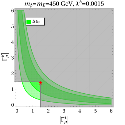
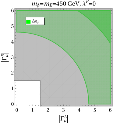
Figure 5: Left panel: allowed region for the coupling strength to the muon $|\Gamma_{\mu}^{L}|$ from the muon anomalous magnetic moment as a function of $|\Gamma_{\mu}^{R}|$, assuming $m_{\phi}=450\,\text{GeV}$, $x^{E}$=1 and $\lambda^{E}=0.0015$. The excluded region due to the requirement of perturbativity for $|\Gamma_{\mu}^{L,R}|$ is given in gray. Dark (light) green corresponds to $1\sigma$ ($2\sigma$) region. The red star marks the benchmark point $(1.5,1.4)$. Right panel: same as the left panel, but assuming $\lambda^{E}=0$.

Also in the quark sector right-handed couplings are needed to address the $B$ anomalies without spoiling at the same time the measurement for $\Delta M_{s}$. This is particularly evident by looking at the left panel of Fig. 6, where the region allowed by both $b\to s\mu^{+}\mu^{-}$ transitions and $B_{s}-{\bar{B}}_{s}$ is shown. Indeed, if one performs a separate fit to $b\to s\mu^{+}\mu^{-}$ transitions and $\Delta M_{s}$ as shown in the right panel of Fig. 6, it is evident that the two channels are incompatible as long as one assumes a vanishing coupling to right-handed bottom and strange quarks, i.e. $\Gamma^{R}=0$.

The preference for non-zero couplings (i.e. beyond the SM effects) is in general driven by $\Delta a_{\mu}$, the angular analyses of $B\to K^{*}\mu^{+}\mu^{-}$ and $B_{s}\to\phi\mu^{+}\mu^{-}$, the branching fraction of $B_{s}\to\mu^{+}\mu^{-}$ and the ratios $R_{K}$ and $R_{K^{*}}$. On the other hand, the experimental constraints coming from $b\to s\gamma$ and $B\to K^{(*)}\nu\bar{\nu}$ and $\Delta M_{B_{s}}$ set bounds on $\Gamma^{L,R}$ and $|\Gamma_{\mu}^{L}|$ that are less stringent than the ones obtained by the inclusion of the aforementioned channels involving $b\to s$ transitions in our setup with $\lambda^{D}_{L,R}=0$. Analogously, the constraints from $Z\to\mu^{+}\mu^{-}$ are found to give negligible constraints on $|\Gamma_{\mu}^{L,R}|$. Concerning $D_{0}-\bar{D_{0}}$ mixing, we recall that Eq. (4.2) implies a relation between $\Gamma^{L}\equiv L^{b}_{1}L_{1}^{s*}$ and $L_{1}^{u,c}$. Exploiting the fact that only the product of $L_{1}^{b}L_{1}^{s*}$ enters $b\to s\ell^{+}\ell^{-}$, together with the suppression of the $L_{1}^{b}$ in $L_{1}^{u,c}$ by small CKM factors ($\mathcal{O}(\lambda^{3})$ and $\mathcal{O}(\lambda^{2})$, respectively), it is possible arrange the contributions to $\Gamma^{L}$ in such a way that the constraint imposed by $D_{0}-\bar{D_{0}}$ mixing is automatically satisfied.

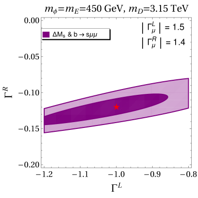
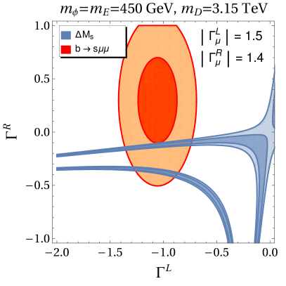
Figure 6: Left panel: Allowed region for the coupling $\Gamma^{L}\equiv\Gamma_{b}^{L}\Gamma_{s}^{L*}$ and $\Gamma^{R}\equiv\Gamma_{b}^{R}\Gamma_{s}^{R*}$ from $B_{s}-\bar{B_{s}}$ mixing and $b\to s\mu^{+}\mu^{-}$ data for $m_{\phi}=m_{E}=450\,\text{GeV}$, $m_{D}=3.15\,\text{TeV}$, $|\Gamma_{\mu}^{L}|=1.5$ and $|\Gamma_{\mu}^{R}|=1.4$. The red star marks the values at our benchmark point $(-1,-0.12)$. The dark (light) purple regions is preferred at the $1\sigma$ ($2\sigma$) level. Right panel: same as the left panel, but showing separately the allowed regions coming from $B_{s}-\bar{B_{s}}$ mixing (in blue) and $b\to s\mu^{+}\mu^{-}$ data (in red). The upper branch allowed by $B_{s}-\bar{B_{s}}$ mixing corresponds to the one shown on the left.

We conclude this section by giving the results for some important observables (within our model) obtained from the global fit, namely

$$R_{K}[1.1,6] = 0.781(45)\,,\quad R_{K^{*}}[1.1,6]=0.885(39)\,,\quad\mathcal{\bar{B}}(B_{s}\to\mu^{+}\mu^{-})=3.30(21)\cdot 10^{-9}\,,$$

$$P_{5}^{\prime}[4,6] = -0.454(69)\,,\qquad\quad P_{5}^{\prime}[6,8]=-0.626(59)\,,$$

$$\Delta a_{\mu} = 235(87)\cdot 10^{-11}\,,\qquad R_{\Delta M_{s}}=-0.02(8)\,.$$ (98)

All the predictions for these observables are compatible at the 1$\sigma$ level with their experimental measurements described in Sec. 3, except for $R_{K^{*}}$ which is compatible only at the $\sim 2\sigma$ level. However, this is expected both from the global fit and from our specific model: As can be seen from the right panel of Fig. 6, there is no overlap of the 1$\sigma$ regions from $b\to s\mu^{+}\mu^{-}$ data and $\Delta M_{s}$ in our model. Furthermore, since our model only allows for NP in muons (neglecting $Z,\gamma$ penguin effects), some small tensions are generated since flavour conserving $b\to s\mu^{+}\mu^{-}$ data prefers a smaller value of $R_{K}$ than the one recently measured.

5 Conclusions and Outlook

In this article we have studied in details the possibility that the intriguing anomalies in $b\to s\ell^{+}\ell^{-}$ processes are explained via box diagrams involving new scalars and fermions. Within this setup we have generalized previous analysis Gripaios:2015gra ; Arnan:2016cpy ; Grinstein:2018fgb to include couplings of the new particles to right-handed SM fermion and calculated the completely general expressions for the Wilson coefficients governing $b\to s$ processes ($b\to s\ell^{+}\ell^{-}$, $b\to s\nu\bar{\nu}$, $b\to s\gamma$ and $B_{s}-\bar{B}_{s}$ mixing). In addition, we have computed the effects in $a_{\mu}$ and $Z\to\mu^{+}\mu^{-}$ which unavoidably arise in such scenarios.

Furthermore, we have proposed a UV complete model containing a $4^{\rm th}$ vector-like generation of fermions and a new scalar, which is capable of explaining $b\to s\ell^{+}\ell^{-}$ data and $a_{\mu}$. We applied the formula derived in our generic setup (see Sec. 2) to this model, illustrating their usefulness. In the following phenomenological analysis of our $4^{\rm th}$ generation model (see Sec. 4.3) we came to the conclusion that the $b\to s\ell^{+}\ell^{-}$ anomalies and $a_{\mu}$ can be explained simultaneously. As a benchmark point which can achieve this, and is consistent with direct LHC searches, we have used $450\,\text{GeV}$ for the vector-like fermions and for the new scalar and $m_{D}=3.15\,\text{TeV}$ for the vector like quarks (with order one couplings). We have observed that right-handed couplings in the muon sector allow to address the long-standing anomaly in $a_{\mu}$ without having to require too large lepton couplings, if one allows for interactions of the vector-like fermions with the SM Higgs. Interestingly, due to the new results from LHCb and BELLE Aaij:2019wad ; Abdesselam:2019wac the global fit to $b\to s\ell^{+}\ell^{-}$ data now prefers non-zero right-handed couplings to quarks and leptons as well, justifying the importance of our generalization of previous analysis performed in this work.

Our $4^{\rm th}$ generation model is also interesting since $\Phi$ is a viable (stable) Dark Matter candidate. We briefly showed that if the mass of $\Phi$ is close to the one of the vector-like leptons, the correct relic density can be obtained while respecting the limits from Dark Matter direct detection. However, a more detailed investigation in the future seems worthwhile.

We conclude observing that our formalism can be directly applied to $b\to d\ell^{+}\ell^{-}$ transitions. In fact, it leads to correlated effects in Kaon physics Crivellin:2016vjc if one aims at explaining the slight tensions in $B\to\pi\mu^{+}\mu^{-}$ Hambrock:2015wka simultaneously with the ones in $b\to s\ell^{+}\ell^{-}$ data. Furthermore, our setup and results can also be used for addressing the tension between theory and experiment in $\epsilon^{\prime}/\epsilon$ Buras:2015yba ; Buras:2018ozh . Here, as a special case of our generic approach, the MSSM has already been studied with the conclusion that it can provide a valid explanation of the anomaly Kitahara:2016otd ; Endo:2016aws ; Crivellin:2017gks .

Note added: After publication of this article, the g-2 collaboration at Fermilab released a new measurement of $a_{\mu}$ Abi:2021gix , which together with the theory consensus of Ref. Aoyama:2020ynm leads to a tension of $4.2\,\sigma$. Furthermore, the LHCb collaboration updated the measurements of $R(K)$ Aaij:2021vac and released the first measurement of $P_{5}^{\prime}$ in $B^{+}\to K^{+*}\mu\mu$ Aaij:2020ruw . Note that this does not change the conclusions of our article and the impact on the numeric is very small. However, this gives additional support to our $4^{\rm th}$ generation model which can account for $(g-2)_{\mu}$ and $B$-anomalies.

Appendix A Fierz Identities

Here we list the Fierz identities for spinors used in the computations. With $i,j,k$ and $l$ representing Dirac indices here we find

$$\left(\gamma_{\mu}P_{L,R}\right)_{ij}\left(\gamma_{\mu}P_{L,R}\right)_{kl} = -\left(\gamma_{\mu}P_{L,R}\right)_{il}\left(\gamma_{\mu}P_{L,R}\right)_{kj}$$ (99)

$$\left(\gamma_{\mu}P_{L,R}\right)_{ij}\left(\gamma_{\mu}P_{R,L}\right)_{kl} = 2\left(P_{R,L}\right)_{il}\left(P_{L,R}\right)_{kj}$$ (100)

$$\left(P_{L,R}\right)_{ij}\left(P_{L,R}\right)_{kl} = \dfrac{1}{2}\left(P_{L,R}\right)_{il}\left(P_{L,R}\right)_{kj}+\dfrac{1}{8}\left(\sigma_{\mu\nu}\right)_{il}\left(\sigma_{\mu\nu}P_{L,R}\right)_{kj}$$ (101)

$$\left(P_{L,R}\right)_{ij}\left(P_{R,L}\right)_{kl} = \dfrac{1}{2}\left(\gamma_{\mu}P_{R,L}\right)_{il}\left(\gamma_{\mu}P_{L,R}\right)_{kj}$$ (102)

$$\left(\sigma_{\mu\nu}\right)_{ij}\left(\sigma_{\mu\nu}P_{L,R}\right)_{kl} = 6\left(\gamma_{\mu}P_{L,R}\right)_{il}\left(\gamma_{\mu}P_{L,R}\right)_{kj}-\dfrac{1}{2}\left(\sigma_{\mu\nu}\right)_{il}\left(\sigma_{\mu\nu}P_{L,R}\right)_{kj}\,,$$ (103)

where $P_{L,R}=\left(1\mp\gamma_{5}\right)/2$ and $\sigma_{\mu\nu}=\frac{i}{2}\left[\gamma_{\mu},\gamma_{\nu}\right]$. When dealing with diagrams with crossed fermion lines, one needs Fierz identities involving charge conjugation matrices. Here, exchanging the second and the third Dirac index we find

$$\left(\gamma_{\mu}P_{L,R}C\right)_{ij}\left(C\gamma_{\mu}P_{L,R}\right)_{kl} = -2\left(P_{R,L}\right)_{ik}\left(P_{L,R}\right)_{jl}$$ (104)

$$\left(\gamma_{\mu}P_{L,R}C\right)_{ij}\left(C\gamma_{\mu}P_{R,L}\right)_{kl} = -\left(\gamma_{\mu}P_{L,R}\right)_{ik}\left(\gamma_{\mu}P_{R,L}\right)_{jl}$$ (105)

$$\left(P_{L,R}C\right)_{ij}\left(CP_{L,R}\right)_{kl} = \dfrac{1}{2}\left(P_{L,R}\right)_{ik}\left(P_{L,R}\right)_{jl}-\dfrac{1}{8}\left(\sigma_{\mu\nu}\right)_{ik}\left(\sigma_{\mu\nu}P_{L,R}\right)_{jl}$$ (106)

$$\left(P_{L,R}C\right)_{ij}\left(CP_{R,L}\right)_{kl} = -\dfrac{1}{2}\left(\gamma_{\mu}P_{R,L}\right)_{ik}\left(\gamma_{\mu}P_{R,L}\right)_{jl}\,,$$ (107)

with the charge conjugation matrix defined as $C=i\gamma_{0}\gamma_{2}$.

Appendix B Loop Functions

Here we list the dimensionless loop functions introduced in Sections 2 and 4. The loop functions appearing in box diagrams that involve four different masses are defined as

$$F(x,y,z) =\frac{x^{2}\log(x)}{(x-1)(x-y)(x-z)}+\frac{y^{2}\log(y)}{(y-1)(y-x)(y-z)}+\frac{z^{2}\log(z)}{(z-1)(z-x)(z-y)}\,,$$ (108)

$$G(x,y,z) =2\left(\frac{x\log(x)}{(x-1)(x-y)(x-z)}+\frac{y\log(y)}{(y-1)(y-x)(y-z)}+\frac{z\log(z)}{(z-1)(z-x)(z-y)}\right)\,,$$

which in the equal mass limit read

$$F(1,1,1)=-G(1,1,1)=\frac{1}{3}\,.$$ (109)

In the presence of only three different masses in the loop, one gets the functions

$$F(x,y) \equiv F(x,y,1)=\frac{1}{(1-x)(1-y)}+\frac{x^{2}\log(x)}{(1-x)^{2}(x-y)}+\frac{y^{2}\log(y)}{(1-y)^{2}(y-x)}\,,$$ (110)

$$G(x,y) \equiv G(x,y,1)=2\left(\frac{1}{(1-x)(1-y)}+\frac{x\log(x)}{(1-x)^{2}(x-y)}+\frac{y\log(y)}{(1-y)^{2}(y-x)}\right)\,,$$

while, in the presence of only two different masses in the loop, one gets

$$F(x) \equiv F(x,x)=\frac{x+1}{(x-1)^{2}}-\dfrac{2x\log(x)}{(x-1)^{3}}\,,$$ (111)

$$G(x) \equiv G(x,x)=\frac{2}{(x-1)^{2}}-\dfrac{(x+1)\log(x)}{(x-1)^{3}}\,.$$

The loop functions appearing in photon- and gluon-penguin diagrams are defined as

$$F_{7}(x) =\dfrac{x^{3}-6x^{2}+3x+2+6x\log x}{12(x-1)^{4}}\,, \widetilde{F}_{7}(x) =x^{-1}F_{7}(x^{-1})\,,$$ (112)

$$G_{7}(x) =\dfrac{x^{2}-4x+3+2\log x}{8(x-1)^{3}}\,, \widetilde{G}_{7}(x) =\frac{x^{2}-2x\log x-1}{8(x-1)^{3}}\,,$$

$$F_{9}(x) =\dfrac{-2x^{3}+9x^{2}-18x+11+6\log x}{36(x-1)^{4}}\,, \widetilde{F}_{9}(x) =x^{-1}F_{9}(x^{-1})\,,$$

$$G_{9}(x) =\dfrac{-16x^{3}+45x^{2}-36x+7+6(2x-3)x^{2}\log x}{36(x-1)^{4}}\,, \widetilde{G}_{9}(x) =x^{-1}G_{9}(x^{-1})\,,$$

which in the equal mass limit read

$$F_{7}(1)=\widetilde{F}_{7}(1)=\frac{G_{7}(1)}{2}=\widetilde{G}_{7}(1)=-F_{9}(1)=-\widetilde{F}_{9}(1)=\frac{G_{9}(1)}{3}=\frac{\widetilde{G}_{9}(1)}{3}=\frac{1}{24}\,.$$ (113)

Finally, the loop functions for the calculation of $Z$-penguins are defined as

$$G_{Z}(x,y) = xF_{V}(x,y)+x\leftrightarrow y\,,$$

$$F_{Z}(x,y,m) \equiv \overline{F}_{Z}(x,y)-\overline{div}_{\varepsilon}=\left(x^{2}F_{V}(x,y)+x\leftrightarrow y\right)-\overline{div}_{\varepsilon}\,,$$

$$H_{Z}(x,y,m) \equiv \overline{H}_{Z}(x,y)+\overline{div}_{\varepsilon}=\left(yF_{V}(x,y)+x\leftrightarrow y\right)+1+\overline{div}_{\varepsilon}\,,$$

$$I_{Z}(x,m) \equiv \overline{I}_{Z}(x)+\overline{div}_{\varepsilon}=\dfrac{x}{x-1}-x^{2}F_{V}(x,1)+\overline{div}_{\varepsilon}\,,$$

$$\widetilde{G}_{Z}(x,y) = xK_{V}(x,y)+x\leftrightarrow y\,,$$

$$\widetilde{F}_{Z}(x,y) = \left(x^{2}K_{V}(x,y)-\frac{x^{2}}{x-y}F_{V}(x,y)\right)+x\leftrightarrow y\,,$$

$$\widetilde{H}_{Z}(x,y) = \left(\dfrac{x^{2}y}{(y-1)(x-y)^{2}}-\dfrac{x^{2}y^{2}(3x-y-2)\log(x)}{(x-1)^{2}(x-y)^{3}}\right)+x\leftrightarrow y\,,$$ (114)

where we have defined $\overline{div}_{\varepsilon}=\Delta_{\varepsilon}-\log\left(\dfrac{m^{2}}{\mu^{2}}\right)$ and

$$F_{V}(x,y)=\frac{\log(x)}{(x-1)(x-y)}\,,\qquad K_{V}(x,y)=\frac{\left(x^{2}+xy-2y\right)\log(x)}{(x-1)^{2}(x-y)^{3}}-\frac{1}{(x-1)(x-y)^{2}}\,.$$

It is interesting to notice that the following relations hold between particular limits of the penguin induced functions:

$$H_{Z}\left(\frac{m^{2}}{n^{2}},\frac{m^{2}}{n^{2}},m\right)=I_{Z}\left(\frac{m^{2}}{n^{2}},n\right)\,,$$

$$-\frac{m^{2}}{n^{2}}G_{Z}\left(\frac{m^{2}}{n^{2}},\frac{m^{2}}{n^{2}}\right)+\frac{1}{2}F_{Z}\left(\frac{m^{2}}{n^{2}},\frac{m^{2}}{n^{2}},n\right)+\frac{1}{4}H_{Z}\left(\frac{m^{2}}{n^{2}},\frac{m^{2}}{n^{2}},m\right)+\frac{1}{4}I_{Z}\left(\frac{m^{2}}{n^{2}},n\right)=0\,,$$

$$\frac{1}{2}x\,\widetilde{G}_{Z}(x,x)-\frac{1}{3}\widetilde{F}_{Z}(x,x)=\widetilde{G}_{9}(x)\,,$$

$$\frac{1}{6}\,\widetilde{F}_{Z}(x,x)=F_{9}(x)\,.$$ (116)

$$\frac{1}{6x}\,\widetilde{H}_{Z}(x,x)=\widetilde{F}_{9}(x)\,.$$ (117)

Moreover, it is useful to define the limit

$$F_{Z}(x)\equiv\overline{F}_{Z}(x,x)=\frac{x}{x-1}+\frac{(x-2)x\log x}{(x-1)^{2}}\,.$$ (118)

Finally, the equal mass limits read

$$G_{Z}(1,1)=\frac{\overline{F}_{Z}(1,1)}{3}=-\overline{H}_{Z}(1,1)=-\overline{I}_{Z}(1)=6\widetilde{G}_{Z}(1,1)=-2\widetilde{F}_{Z}(1,1)=-2\widetilde{H}_{Z}(1,1)=\frac{1}{2}\,.$$ (119)

Appendix C Real Scalars and Majorana Fermions

If the NP fields have the appropriate quantum numbers they can be either real scalars or Majorana fermions. If this is the case, crossed diagrams as shown in Fig. 7 can be constructed and contribute to $b\to s\mu^{+}\mu^{-}$ transitions in addition to the ones shown in Fig. 1. Similarly, there are contributions from crossed boxes to $B_{s}-\bar{B}_{s}$ mixing (in addition to the ones in Fig. 3) arising due to the diagrams in Fig. 8.

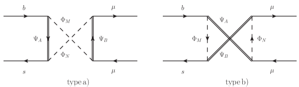
Figure 7: Crossed box diagrams contributing to $b\to s\mu^{+}\mu^{-}$ transitions. The diagram on the left appears in models with real scalars, while the one on the right can be constructed in models with Majorana fermions.

$SU(3)$, type $a)$	$\Psi_{A}$	$\Psi_{B}$	$\Phi_{M}$	$\Phi_{N}$	$SU(3)$, type $b)$	$\Psi_{A}$	$\Psi_{B}$	$\Phi_{M}$	$\Phi_{N}$	$\chi$
I	3	1	1	1	I	1	1	3	1	1
III	3	8	8	8	III	8	8	3	8	4/3

Table 5: Table of $SU(3)$-factors entering the box induced Wilson coefficients involved in $b\to s$ transitions for real scalars, type $a)$, and Majorana fermions, type $b)$. The numbers of each representation refer to the ones in Table 1.

C.1 $b\to s\mu^{+}\mu^{-}$

In $b\to s\mu^{+}\mu^{-}$ the possible representations that give rise to additional crossed diagrams with real scalars or Majorana fermions are listed in Tab. 5. For type $a)$ the only possibility is to have real scalars, while for type $b)$ one can only have crossed diagrams in the presence of Majorana fermions.

The contribution to the Wilson coefficients stemming from the diagrams in Fig. 7$a)$ corresponds to the ones listed for $a)$-type in Eqs. (4)-(7), after inverting $M\leftrightarrow N$ in the muon couplings and changing $F(x_{AM},x_{BM},x_{NM})\to-F(x_{AM},x_{BM},x_{NM})$. For case $b)$ (see right diagram in Fig. 7) the Wilson coefficients are given by

$$C_{9}^{{\text{box}}\;b)} = -{\cal N}\frac{\chi L^{s*}_{BM}L^{b}_{AM}}{{32\pi\alpha_{\text{EM}}m_{\Phi_{M}}^{2}}}\bigg{[}L^{\mu*}_{BN}L^{\mu}_{AN}\frac{m_{\Psi_{A}}m_{\Psi_{B}}}{m_{\Phi_{M}}^{2}}G(x_{AM},x_{BM},x_{NM})$$ (120)

$$\qquad\qquad\qquad\qquad-R^{\mu*}_{BN}R^{\mu}_{AN}F(x_{AM},x_{BM},x_{NM})\bigg{]}\,,$$

$$C_{10}^{{\text{box}}\;b)} = {\cal N}\frac{\chi L^{s*}_{BM}L^{b}_{AM}}{{32\pi\alpha_{\text{EM}}m_{\Phi_{M}}^{2}}}\bigg{[}L^{\mu*}_{BN}L^{\mu}_{AN}\frac{m_{\Psi_{A}}m_{\Psi_{B}}}{m_{\Phi_{M}}^{2}}G(x_{AM},x_{BM},x_{NM})$$ (121)

$$\qquad\qquad\qquad\quad+R^{\mu*}_{BN}R^{\mu}_{AN}F(x_{AM},x_{BM},x_{NM})\bigg{]}\,,$$

$$C_{S}^{{\text{box}}\;b)} = {\cal N}\frac{\chi L^{s*}_{BM}L^{b}_{AM}}{{16\pi\alpha_{\text{EM}}m_{\Phi_{M}}^{2}}}\bigg{[}R^{\mu*}_{BN}L^{\mu}_{AN}F(x_{AM},x_{BM},x_{NM})$$ (122)

$$\qquad\qquad\qquad\quad+L^{\mu*}_{BN}R^{\mu}_{AN}\frac{m_{\Psi_{A}}m_{\Psi_{B}}}{2m_{\Phi_{M}}^{2}}G(x_{AM},x_{BM},x_{NM})\bigg{]}\,,$$

$$C_{P}^{{\text{box}}\;b)} = {\cal N}\frac{\chi L^{s*}_{BM}L^{b}_{AM}}{{16\pi\alpha_{\text{EM}}m_{\Phi_{M}}^{2}}}\bigg{[}R^{\mu*}_{BN}L^{\mu}_{AN}F(x_{AM},x_{BM},x_{NM})$$ (123)

$$\qquad\qquad\qquad\quad-L^{\mu*}_{BN}R^{\mu}_{AN}\frac{m_{\Psi_{A}}m_{\Psi_{B}}}{2m_{\Phi_{M}}^{2}}G(x_{AM},x_{BM},x_{NM})\bigg{]}\,,$$

$$C_{T}^{{\text{box}}\;b)} = -{\cal N}\frac{\chi L^{s*}_{BM}R^{b}_{AM}L^{\mu*}_{BN}R^{\mu}_{AN}}{{16\pi\alpha_{\text{EM}}m_{\Phi_{M}}^{2}}}\frac{m_{\Psi_{A}}m_{\Psi_{B}}}{m_{\Phi_{M}}^{2}}G(x_{AM},x_{BM},x_{NM})\,,$$ (124)

$$C_{9,S}^{\prime\text{box}\,}=C_{9,S}^{\text{box}\,}\left(L\leftrightarrow R\right)\,,\qquad C_{P,10}^{\prime\text{box}\,}=-C_{P,10}^{\text{box}\,}\left(L\leftrightarrow R\right)\,,$$ (125)

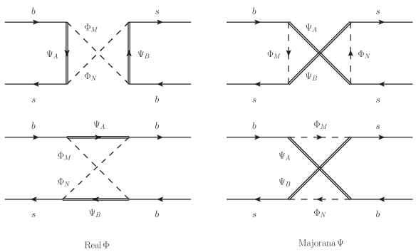
Figure 8: Box diagrams contributing to $B_{s}-\bar{B}_{s}$ mixing. The diagram on the left is relative to models with real scalars, while the one on the right refers to models with Majorana fermions.

$SU(3)$	$\Psi_{A}$	$\Psi_{B}$	$\Phi_{M}$	$\Phi_{N}$	$\chi_{BB}^{M}$	$\tilde{\chi}_{BB}^{M}$
I	3	3	1	1	1	0	Real $\Phi$
II	1	1	3	3	0	1	Majorana $\Psi$
III	3	3	8	8	5/18	-1/6	Real $\Phi$
IV	8	8	3	3	-1/6	5/18	Majorana $\Psi$
V	3	3	(1,8)	(8,1)	1/6	-1/2	Real $\Phi$
VI	(1,8)	(8,1)	3	3	-1/2	1/6	Majorana $\Psi$

Table 6: Table of $SU(3)$-factors entering the box induced Wilson coefficients involved in $B_{s}-\bar{B}_{s}$ mixing for real scalars and Majorana fermions.

C.2 $B_{s}-\bar{B_{s}}$ mixing

For $B_{s}$ mixing we can either have real scalars or Majorana fermions. In Tab. 6 we list the possible representations of the diagrams in Fig. 8 writing explicitly if we have a real scalar contribution (diagrams on the left side of the figure) or a Majorana fermion (diagrams on the right). The WCs for real scalar crossed diagrams correspond to the ones listed in Eqs. (4)-(7), after inverting $M\leftrightarrow N$ in two of the four couplings and changing $F(x_{AM},x_{BM},x_{NM})\to-F(x_{AM},x_{BM},x_{NM})$, whereas matching to the generic Lagrangian from Eq. (1) with the crossed fermion contributions, one obtains the following results for the coefficients:

$$C_{1} = (\chi_{BB}^{M}+\tilde{\chi}_{BB}^{M})\frac{L^{s*}_{AN}L^{b}_{BM}L^{s*}_{AM}L^{b}_{BN}}{128\pi^{2}m_{\Phi_{M}}^{2}}\frac{m_{\Psi_{A}}m_{\Psi_{B}}}{m_{\Phi_{M}}^{2}}G\left(x_{AM},x_{BM},x_{NM}\right)\,,$$ (126)

$$C_{2,3} = -(\chi_{BB}^{M}+\tilde{\chi}_{BB}^{M})\frac{R^{s*}_{AN}L^{b}_{BM}R^{s*}_{AM}L^{b}_{BN}}{64\pi^{2}m_{\Phi_{M}}^{2}}\frac{m_{\Psi_{A}}m_{\Psi_{B}}}{m_{\Phi_{M}}^{2}}G\left(x_{AM},x_{BM},x_{NM}\right)\,,$$ (127)

$$C_{4} = \frac{L^{b}_{AM}R^{b}_{AN}}{32\pi^{2}m_{\Phi_{M}}^{2}}\left[\chi_{BB}^{M}L^{s*}_{BM}R^{s*}_{BN}-\tilde{\chi}_{BB}^{M}R^{s*}_{BM}L^{s*}_{BN}\right]F\left(x_{AM},x_{BM},x_{NM}\right)\,,\qquad$$ (128)

$$C_{5} = \frac{L^{b}_{AM}R^{b}_{AN}}{32\pi^{2}m_{\Phi_{M}}^{2}}\left[\tilde{\chi}_{BB}^{M}L^{s*}_{BM}R^{s*}_{BN}-\chi_{BB}^{M}R^{s*}_{BM}L^{s*}_{BN}\right]F\left(x_{AM},x_{BM},x_{NM}\right)\,,\qquad$$ (129)

$$\widetilde{C}_{i} = C_{i}\left(L\to R\right)\,,\qquad\text{for}\qquad i=\{1,2,3\}\,,$$ (130)

The corresponding contributions to $D_{0}-\overline{D}_{0}$ mixing are obtained from Eqs. (22)-(28) via the replacements $s\to u$ and $b\to c$.

Appendix D Crossed Diagrams with Complex Scalars

There is also the possibility that a complex scalar couples to the down-type quarks whereas its hermitian conjugated version couples to muons. This means that the Lagrangian in Eq. (1) takes a slightly different form, namely

$$\mathcal{L}_{\rm int}= \bigg{[} \bar{\Psi}_{A}\left(L_{AM}^{b}{P_{L}}{b}+L_{AM}^{s}{P_{L}}{s}+{R_{AM}^{b}}{P_{R}}{b}+R_{AM}^{s}{P_{R}}{s}\right){\Phi_{M}}$$ (131)

$$+\bar{\Psi}_{A}\left(L_{AM}^{\mu}{P_{L}}+{R_{AM}^{\mu}{P_{R}}\mu}\right){\Phi_{M}^{\dagger}}\bigg{]}+\mathrm{h.c.}\,.$$

Also this Lagrangian generates a contribution to $b\to s\mu^{+}\mu^{-}$ via the diagram shown in Fig. 9. The possible representations under the $SU(3)$ of the new scalars and fermions in the loop are listed in Tab. 7. The corresponding Wilson Coefficients can be obtained from the ones calculated for the type $b)$ diagrams in Eqs. (4)-(7) by exchanging $M\leftrightarrow N$ in the couplings $R,L$ and replacing $F(x_{AM},x_{BM},x_{NM})\rightarrow-F(x_{AM},x_{BM},x_{NM})$.

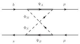
Figure 9: Crossed box diagrams contributing to $b\to s\mu^{+}\mu^{-}$ transitions. The diagram appears when a complex scalar couples to $b,s$ quarks and its conjugate couples to the muons.

$SU(3)$	$\Psi_{A}$	$\Psi_{B}$	$\Phi_{M}$	$\Phi_{N}$	$\chi$
I	(1,3)	(3,1)	($\bar{3}$,1)	(1,$\bar{3}$)	1
II	(8,3)	(3,8)	($\bar{3}$,8)	(8,$\bar{3}$)	4/3
III	$\bar{3}$	$\bar{3}$	3	3	2

Table 7: Table of $SU(3)$-factors entering the box induced Wilson coefficients involved in $b\to s$ transitions for crossed diagrams with complex scalars.

Appendix E Posterior Distributions

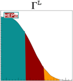
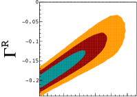
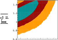
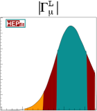
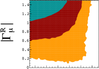
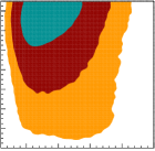
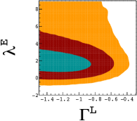
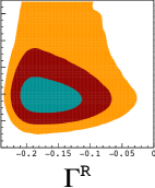
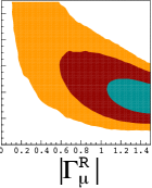
Figure 10: The $1D$ marginalized posterior distributions of the parameters from the fit described in sec. 4.2, together with the $2D$ correlations between them. The green, red and orange regions correspond to $68\%$, $95\%$ and $99\%$ probability regions, respectively.

Here we show the $1D$ marginalized posterior distributions of the parameters from the global fit described in Sec. 4.2, together with the $2D$ combined correlations between these parameters. The results are summarized in Fig. 10. We recall that, for all couplings $\Gamma$, we imposed $|\Gamma|\leq 1.5$ such that perturbativity is satisfied. The consequences of such this choice are evident in the posterior distributions of $\Gamma^{L}$, $|\Gamma^{L}_{\mu}|$ and $|\Gamma^{R}_{\mu}|$, which are truncated because of this reason.

References

• (1) B. Capdevila, A. Crivellin, S. Descotes-Genon, J. Matias and J. Virto, Patterns of New Physics in $b\to s\ell^{+}\ell^{-}$ transitions in the light of recent data, JHEP 01 (2018) 093 [1704.05340].
• (2) W. Altmannshofer, P. Stangl and D. M. Straub, Interpreting Hints for Lepton Flavor Universality Violation, Phys. Rev. D96 (2017) 055008 [1704.05435].
• (3) G. D’Amico, M. Nardecchia, P. Panci, F. Sannino, A. Strumia, R. Torre et al., Flavour anomalies after the $R_{K^{*}}$ measurement, JHEP 09 (2017) 010 [1704.05438].
• (4) G. Hiller and I. Nisandzic, $R_{K}$ and $R_{K^{\ast}}$ beyond the standard model, Phys. Rev. D96 (2017) 035003 [1704.05444].
• (5) L.-S. Geng, B. Grinstein, S. Jäger, J. Martin Camalich, X.-L. Ren and R.-X. Shi, Towards the discovery of new physics with lepton-universality ratios of $b\to s\ell\ell$ decays, Phys. Rev. D96 (2017) 093006 [1704.05446].
• (6) M. Ciuchini, A. M. Coutinho, M. Fedele, E. Franco, A. Paul, L. Silvestrini et al., On Flavourful Easter eggs for New Physics hunger and Lepton Flavour Universality violation, Eur. Phys. J. C77 (2017) 688 [1704.05447].
• (7) A. K. Alok, B. Bhattacharya, A. Datta, D. Kumar, J. Kumar and D. London, New Physics in $b\to s\mu^{+}\mu^{-}$ after the Measurement of $R_{K^{*}}$, Phys. Rev. D96 (2017) 095009 [1704.07397].
• (8) T. Hurth, F. Mahmoudi, D. Martinez Santos and S. Neshatpour, Lepton nonuniversality in exclusive $b{\rightarrow}s{\ell}{\ell}$ decays, Phys. Rev. D96 (2017) 095034 [1705.06274].
• (9) LHCb collaboration, Search for lepton-universality violation in $B^{+}\to K^{+}\ell^{+}\ell^{-}$ decays, 1903.09252.
• (10) Belle collaboration, Test of lepton flavor universality in ${B\to K^{\ast}\ell^{+}\ell^{-}}$ decays at Belle, 1904.02440.
• (11) Heavy Flavor Averaging Group collaboration, Averages of $b$-hadron, $c$-hadron, and $\tau$-lepton properties as of summer 2016, Eur. Phys. J. C77 (2017) 895 [1612.07233].
• (12) M. Algueró, B. Capdevila, A. Crivellin, S. Descotes-Genon, P. Masjuan, J. Matias et al., Addendum: ”Patterns of New Physics in $b\to s\ell^{+}\ell^{-}$ transitions in the light of recent data” and ”Are we overlooking Lepton Flavour Universal New Physics in $b\to s\ell\ell\,$?”, 1903.09578.
• (13) A. K. Alok, A. Dighe, S. Gangal and D. Kumar, Continuing search for new physics in $b\to s\mu\mu$ decays: two operators at a time, 1903.09617.
• (14) M. Ciuchini, A. M. Coutinho, M. Fedele, E. Franco, A. Paul, L. Silvestrini et al., New Physics in $b\to s\ell^{+}\ell^{-}$ confronts new data on Lepton Universality, 1903.09632.
• (15) A. Datta, J. Kumar and D. London, The $B$ Anomalies and New Physics in $b\to se^{+}e^{-}$, 1903.10086.
• (16) J. Aebischer, W. Altmannshofer, D. Guadagnoli, M. Reboud, P. Stangl and D. M. Straub, B-decay discrepancies after Moriond 2019, 1903.10434.
• (17) K. Kowalska, D. Kumar and E. M. Sessolo, Implications for New Physics in $b\to s\mu\mu$ transitions after recent measurements by Belle and LHCb, 1903.10932.
• (18) S. Descotes-Genon, J. Matias and J. Virto, Understanding the $B\to K^{*}\mu^{+}\mu^{-}$ Anomaly, Phys. Rev. D88 (2013) 074002 [1307.5683].
• (19) R. Gauld, F. Goertz and U. Haisch, An explicit Z’-boson explanation of the $B\to K^{*}\mu^{+}\mu^{-}$ anomaly, JHEP 01 (2014) 069 [1310.1082].
• (20) A. J. Buras, F. De Fazio and J. Girrbach, 331 models facing new $b\to s\mu^{+}\mu^{-}$ data, JHEP 02 (2014) 112 [1311.6729].
• (21) W. Altmannshofer, S. Gori, M. Pospelov and I. Yavin, Quark flavor transitions in $L_{\mu}-L_{\tau}$ models, Phys. Rev. D89 (2014) 095033 [1403.1269].
• (22) A. Crivellin, G. D’Ambrosio and J. Heeck, Explaining $h\to\mu^{\pm}\tau^{\mp}$, $B\to K^{*}\mu^{+}\mu^{-}$ and $B\to K\mu^{+}\mu^{-}/B\to Ke^{+}e^{-}$ in a two-Higgs-doublet model with gauged $L_{\mu}-L_{\tau}$, Phys. Rev. Lett. 114 (2015) 151801 [1501.00993].
• (23) A. Crivellin, G. D’Ambrosio and J. Heeck, Addressing the LHC flavor anomalies with horizontal gauge symmetries, Phys. Rev. D91 (2015) 075006 [1503.03477].
• (24) C. Niehoff, P. Stangl and D. M. Straub, Violation of lepton flavour universality in composite Higgs models, Phys. Lett. B747 (2015) 182 [1503.03865].
• (25) D. Aristizabal Sierra, F. Staub and A. Vicente, Shedding light on the $b\to s$ anomalies with a dark sector, Phys. Rev. D92 (2015) 015001 [1503.06077].
• (26) A. Crivellin, L. Hofer, J. Matias, U. Nierste, S. Pokorski and J. Rosiek, Lepton-flavour violating $B$ decays in generic $Z^{\prime}$ models, Phys. Rev. D92 (2015) 054013 [1504.07928].
• (27) A. Celis, J. Fuentes-Martin, M. Jung and H. Serodio, Family nonuniversal Z’ models with protected flavor-changing interactions, Phys. Rev. D92 (2015) 015007 [1505.03079].
• (28) B. Allanach, F. S. Queiroz, A. Strumia and S. Sun, $Z^{\prime}$ models for the LHCb and $g-2$ muon anomalies, Phys. Rev. D93 (2016) 055045 [1511.07447].
• (29) D. Bečirević, O. Sumensari and R. Zukanovich Funchal, Lepton flavor violation in exclusive $b\rightarrow s$ decays, Eur. Phys. J. C76 (2016) 134 [1602.00881].
• (30) A. Celis, W.-Z. Feng and M. Vollmann, Dirac dark matter and $b\to s\ell^{+}\ell^{-}$ with $\mathrm{U(1)}$ gauge symmetry, Phys. Rev. D95 (2017) 035018 [1608.03894].
• (31) S. M. Boucenna, A. Celis, J. Fuentes-Martin, A. Vicente and J. Virto, Non-abelian gauge extensions for B-decay anomalies, Phys. Lett. B760 (2016) 214 [1604.03088].
• (32) S. M. Boucenna, A. Celis, J. Fuentes-Martin, A. Vicente and J. Virto, Phenomenology of an $SU(2)\times SU(2)\times U(1)$ model with lepton-flavour non-universality, JHEP 12 (2016) 059 [1608.01349].
• (33) E. Megias, G. Panico, O. Pujolas and M. Quiros, A Natural origin for the LHCb anomalies, JHEP 09 (2016) 118 [1608.02362].
• (34) W. Altmannshofer, S. Gori, S. Profumo and F. S. Queiroz, Explaining dark matter and B decay anomalies with an $L_{\mu}-L_{\tau}$ model, JHEP 12 (2016) 106 [1609.04026].
• (35) A. Crivellin, J. Fuentes-Martin, A. Greljo and G. Isidori, Lepton Flavor Non-Universality in B decays from Dynamical Yukawas, Phys. Lett. B766 (2017) 77 [1611.02703].
• (36) S. Di Chiara, A. Fowlie, S. Fraser, C. Marzo, L. Marzola, M. Raidal et al., Minimal flavor-changing $Z^{\prime}$ models and muon $g-2$ after the $R_{K^{*}}$ measurement, Nucl. Phys. B923 (2017) 245 [1704.06200].
• (37) C.-W. Chiang, X.-G. He, J. Tandean and X.-B. Yuan, $R_{K^{(*)}}$ and related $b\to s\ell\bar{\ell}$ anomalies in minimal flavor violation framework with $Z^{\prime}$ boson, Phys. Rev. D96 (2017) 115022 [1706.02696].
• (38) M. Crispim Romao, S. F. King and G. K. Leontaris, Non-universal $Z^{\prime}$ from fluxed GUTs, Phys. Lett. B782 (2018) 353 [1710.02349].
• (39) L. Bian, H. M. Lee and C. B. Park, $B$-meson anomalies and Higgs physics in flavored $U(1)^{\prime}$ model, Eur. Phys. J. C78 (2018) 306 [1711.08930].
• (40) A. Falkowski, S. F. King, E. Perdomo and M. Pierre, Flavourful $Z^{\prime}$ portal for vector-like neutrino Dark Matter and $R_{K^{(*)}}$, JHEP 08 (2018) 061 [1803.04430].
• (41) D. Guadagnoli, M. Reboud and O. Sumensari, A gauged horizontal $SU(2)$ symmetry and $R_{K^{(\ast)}}$, JHEP 11 (2018) 163 [1807.03285].
• (42) B. Gripaios, M. Nardecchia and S. A. Renner, Composite leptoquarks and anomalies in $B$-meson decays, JHEP 05 (2015) 006 [1412.1791].
• (43) D. Bečirević, S. Fajfer and N. Košnik, Lepton flavor nonuniversality in $b\to s\ell^{+}\ell^{-}$ processes, Phys. Rev. D92 (2015) 014016 [1503.09024].
• (44) I. de Medeiros Varzielas and G. Hiller, Clues for flavor from rare lepton and quark decays, JHEP 06 (2015) 072 [1503.01084].
• (45) R. Alonso, B. Grinstein and J. Martin Camalich, Lepton universality violation and lepton flavor conservation in $B$-meson decays, JHEP 10 (2015) 184 [1505.05164].
• (46) L. Calibbi, A. Crivellin and T. Ota, Effective Field Theory Approach to $b\to s\ell\ell^{(\prime)},B\to K^{(*)}\nu\overline{\nu}$ and $B\to D^{(*)}\tau\nu$ with Third Generation Couplings, Phys. Rev. Lett. 115 (2015) 181801 [1506.02661].
• (47) G. Bélanger, C. Delaunay and S. Westhoff, A Dark Matter Relic From Muon Anomalies, Phys. Rev. D92 (2015) 055021 [1507.06660].
• (48) R. Barbieri, G. Isidori, A. Pattori and F. Senia, Anomalies in $B$-decays and $U(2)$ flavour symmetry, Eur. Phys. J. C76 (2016) 67 [1512.01560].
• (49) D. Bečirević, N. Košnik, O. Sumensari and R. Zukanovich Funchal, Palatable Leptoquark Scenarios for Lepton Flavor Violation in Exclusive $b\to s\ell_{1}\ell_{2}$ modes, JHEP 11 (2016) 035 [1608.07583].
• (50) D. Bečirević, S. Fajfer, N. Košnik and O. Sumensari, Leptoquark model to explain the $B$-physics anomalies, $R_{K}$ and $R_{D}$, Phys. Rev. D94 (2016) 115021 [1608.08501].
• (51) S. Sahoo, R. Mohanta and A. K. Giri, Explaining the $R_{K}$ and $R_{D^{(*)}}$ anomalies with vector leptoquarks, Phys. Rev. D95 (2017) 035027 [1609.04367].
• (52) G. Hiller, D. Loose and K. Schönwald, Leptoquark Flavor Patterns & B Decay Anomalies, JHEP 12 (2016) 027 [1609.08895].
• (53) P. Cox, A. Kusenko, O. Sumensari and T. T. Yanagida, SU(5) Unification with TeV-scale Leptoquarks, JHEP 03 (2017) 035 [1612.03923].
• (54) A. Crivellin, D. Müller and T. Ota, Simultaneous explanation of R(D(∗)) and $b\to s\mu^{+}\mu^{-}$: the last scalar leptoquarks standing, JHEP 09 (2017) 040 [1703.09226].
• (55) Y. Cai, J. Gargalionis, M. A. Schmidt and R. R. Volkas, Reconsidering the One Leptoquark solution: flavor anomalies and neutrino mass, JHEP 10 (2017) 047 [1704.05849].
• (56) I. Doršner, S. Fajfer, D. A. Faroughy and N. Košnik, The role of the $S_{3}$ GUT leptoquark in flavor universality and collider searches, 1706.07779.
• (57) D. Buttazzo, A. Greljo, G. Isidori and D. Marzocca, B-physics anomalies: a guide to combined explanations, JHEP 11 (2017) 044 [1706.07808].
• (58) N. Assad, B. Fornal and B. Grinstein, Baryon Number and Lepton Universality Violation in Leptoquark and Diquark Models, Phys. Lett. B777 (2018) 324 [1708.06350].
• (59) L. Di Luzio, A. Greljo and M. Nardecchia, Gauge leptoquark as the origin of B-physics anomalies, Phys. Rev. D96 (2017) 115011 [1708.08450].
• (60) L. Calibbi, A. Crivellin and T. Li, Model of vector leptoquarks in view of the $B$-physics anomalies, Phys. Rev. D98 (2018) 115002 [1709.00692].
• (61) M. Bordone, C. Cornella, J. Fuentes-Martin and G. Isidori, A three-site gauge model for flavor hierarchies and flavor anomalies, Phys. Lett. B779 (2018) 317 [1712.01368].
• (62) M. Blanke and A. Crivellin, $B$ Meson Anomalies in a Pati-Salam Model within the Randall-Sundrum Background, Phys. Rev. Lett. 121 (2018) 011801 [1801.07256].
• (63) D. Marzocca, Addressing the B-physics anomalies in a fundamental Composite Higgs Model, JHEP 07 (2018) 121 [1803.10972].
• (64) M. Bordone, C. Cornella, J. Fuentes-Martín and G. Isidori, Low-energy signatures of the $\mathrm{PS}^{3}$ model: from $B$-physics anomalies to LFV, JHEP 10 (2018) 148 [1805.09328].
• (65) D. Bečirević, I. Doršner, S. Fajfer, N. Košnik, D. A. Faroughy and O. Sumensari, Scalar leptoquarks from grand unified theories to accommodate the $B$-physics anomalies, Phys. Rev. D98 (2018) 055003 [1806.05689].
• (66) A. Crivellin, C. Greub, D. Müller and F. Saturnino, Importance of Loop Effects in Explaining the Accumulated Evidence for New Physics in B Decays with a Vector Leptoquark, Phys. Rev. Lett. 122 (2019) 011805 [1807.02068].
• (67) I. de Medeiros Varzielas and S. F. King, ${R}_{K^{\left(*\right)}}$ with leptoquarks and the origin of Yukawa couplings, JHEP 11 (2018) 100 [1807.06023].
• (68) L. Di Luzio, J. Fuentes-Martin, A. Greljo, M. Nardecchia and S. Renner, Maximal Flavour Violation: a Cabibbo mechanism for leptoquarks, JHEP 11 (2018) 081 [1808.00942].
• (69) T. Faber, M. Hudec, M. Malinský, P. Meinzinger, W. Porod and F. Staub, A unified leptoquark model confronted with lepton non-universality in $B$-meson decays, Phys. Lett. B787 (2018) 159 [1808.05511].
• (70) J. Heeck and D. Teresi, Pati-Salam explanations of the B-meson anomalies, JHEP 12 (2018) 103 [1808.07492].
• (71) A. Angelescu, D. Bečirević, D. A. Faroughy and O. Sumensari, Closing the window on single leptoquark solutions to the $B$-physics anomalies, JHEP 10 (2018) 183 [1808.08179].
• (72) V. Gherardi, D. Marzocca, M. Nardecchia and A. Romanino, Rank-One Flavor Violation and B-meson anomalies, 1903.10954.
• (73) C. Cornella, J. Fuentes-Martin and G. Isidori, Revisiting the vector leptoquark explanation of the B-physics anomalies, 1903.11517.
• (74) C. Bobeth, A. J. Buras, A. Celis and M. Jung, Patterns of Flavour Violation in Models with Vector-Like Quarks, JHEP 04 (2017) 079 [1609.04783].
• (75) S.-P. Li, X.-Q. Li, Y.-D. Yang and X. Zhang, ${R}_{D^{\left(*\right)}},{R}_{K^{\left(*\right)}}$ and neutrino mass in the 2HDM-III with right-handed neutrinos, JHEP 09 (2018) 149 [1807.08530].
• (76) C. Marzo, L. Marzola and M. Raidal, Common explanation to the $R_{K^{(*)}}$, $R_{D^{(*)}}$ and $\epsilon^{\prime}/\epsilon$ anomalies in a 3HDM+$\nu_{R}$ and connections to neutrino physics, 1901.08290.
• (77) A. Crivellin, D. Müller and C. Wiegand, $b\to s\ell^{+}\ell^{-}$ Transitions in Two-Higgs-Doublet Models, 1903.10440.
• (78) B. Gripaios, M. Nardecchia and S. A. Renner, Linear flavour violation and anomalies in B physics, JHEP 06 (2016) 083 [1509.05020].
• (79) P. Arnan, L. Hofer, F. Mescia and A. Crivellin, Loop effects of heavy new scalars and fermions in $b\to s\mu^{+}\mu^{-}$, JHEP 04 (2017) 043 [1608.07832].
• (80) B. Barman, D. Borah, L. Mukherjee and S. Nandi, Correlating the anomalous results in $b\to s$ decays with inert Higgs doublet dark matter and muon $(g-2)$, 1808.06639.
• (81) B. Grinstein, S. Pokorski and G. G. Ross, Lepton non-universality in $B$ decays and fermion mass structure, JHEP 12 (2018) 079 [1809.01766].
• (82) D. Bečirević and O. Sumensari, A leptoquark model to accommodate $R_{K}^{\mathrm{exp}}<R_{K}^{\mathrm{SM}}$ and $R_{K^{\ast}}^{\mathrm{exp}}<R_{K^{\ast}}^{\mathrm{SM}}$, JHEP 08 (2017) 104 [1704.05835].
• (83) J. F. Kamenik, Y. Soreq and J. Zupan, Lepton flavor universality violation without new sources of quark flavor violation, Phys. Rev. D97 (2018) 035002 [1704.06005].
• (84) J. E. Camargo-Molina, A. Celis and D. A. Faroughy, Anomalies in Bottom from new physics in Top, Phys. Lett. B784 (2018) 284 [1805.04917].
• (85) J. Aebischer, A. Crivellin, M. Fael and C. Greub, Matching of gauge invariant dimension-six operators for $b\to s$ and $b\to c$ transitions, JHEP 05 (2016) 037 [1512.02830].
• (86) S. Baek, Dark matter contribution to $b\to s\mu^{+}\mu^{-}$ anomaly in local $U(1)_{L_{\mu}-L_{\tau}}$ model, Phys. Lett. B781 (2018) 376 [1707.04573].
• (87) J. Kawamura, S. Okawa and Y. Omura, Interplay between the b$\to s\ell\ell$ anomalies and dark matter physics, Phys. Rev. D96 (2017) 075041 [1706.04344].
• (88) C.-W. Chiang and H. Okada, A simple model for explaining muon-related anomalies and dark matter, 1711.07365.
• (89) J. M. Cline and J. M. Cornell, $R({K^{(*)}})$ from dark matter exchange, Phys. Lett. B782 (2018) 232 [1711.10770].
• (90) S. Baek and C. Yu, Dark matter for $b\to s\mu^{+}\mu^{-}$ anomaly in a gauged $U(1)_{X}$ model, JHEP 11 (2018) 054 [1806.05967].
• (91) S. Baek, Scalar dark matter behind $b\to s\mu\mu$ anomaly, 1901.04761.
• (92) D. G. Cerdeño, A. Cheek, P. Martín-Ramiro and J. M. Moreno, B anomalies and dark matter: a complex connection, 1902.01789.
• (93) Muon g-2 collaboration, Final Report of the Muon E821 Anomalous Magnetic Moment Measurement at BNL, Phys. Rev. D73 (2006) 072003 [hep-ex/0602035].
• (94) A. Crivellin, M. Hoferichter and P. Schmidt-Wellenburg, Combined explanations of $(g-2)_{\mu,e}$ and implications for a large muon EDM, Phys. Rev. D98 (2018) 113002 [1807.11484].
• (95) F. del Aguila, J. de Blas and M. Perez-Victoria, Effects of new leptons in Electroweak Precision Data, Phys. Rev. D78 (2008) 013010 [0803.4008].
• (96) K. Kannike, M. Raidal, D. M. Straub and A. Strumia, Anthropic solution to the magnetic muon anomaly: the charged see-saw, JHEP 02 (2012) 106 [1111.2551].
• (97) A. Joglekar, P. Schwaller and C. E. M. Wagner, Dark Matter and Enhanced Higgs to Di-photon Rate from Vector-like Leptons, JHEP 12 (2012) 064 [1207.4235].
• (98) J. Kearney, A. Pierce and N. Weiner, Vectorlike Fermions and Higgs Couplings, Phys. Rev. D86 (2012) 113005 [1207.7062].
• (99) K. Ishiwata and M. B. Wise, Phenomenology of heavy vectorlike leptons, Phys. Rev. D88 (2013) 055009 [1307.1112].
• (100) R. Dermisek and A. Raval, Explanation of the Muon g-2 Anomaly with Vectorlike Leptons and its Implications for Higgs Decays, Phys. Rev. D88 (2013) 013017 [1305.3522].
• (101) K. Kowalska and E. M. Sessolo, Expectations for the muon g-2 in simplified models with dark matter, JHEP 09 (2017) 112 [1707.00753].
• (102) L. Calibbi, R. Ziegler and J. Zupan, Minimal models for dark matter and the muon g-2 anomaly, JHEP 07 (2018) 046 [1804.00009].
• (103) Z. Poh and S. Raby, Vectorlike leptons: Muon g-2 anomaly, lepton flavor violation, Higgs boson decays, and lepton nonuniversality, Phys. Rev. D96 (2017) 015032 [1705.07007].
• (104) S. Raby and A. Trautner, Vectorlike chiral fourth family to explain muon anomalies, Phys. Rev. D97 (2018) 095006 [1712.09360].
• (105) G. C. Branco and L. Lavoura, On the Addition of Vector Like Quarks to the Standard Model, Nucl. Phys. B278 (1986) 738.
• (106) F. del Aguila, L. Ametller, G. L. Kane and J. Vidal, Vector Like Fermion and Standard Higgs Production at Hadron Colliders, Nucl. Phys. B334 (1990) 1.
• (107) P. Langacker and D. London, Mixing Between Ordinary and Exotic Fermions, Phys. Rev. D38 (1988) 886.
• (108) F. del Aguila, J. A. Aguilar-Saavedra and G. C. Branco, CP violation from new quarks in the chiral limit, Nucl. Phys. B510 (1998) 39 [hep-ph/9703410].
• (109) MEG collaboration, Search for the lepton flavour violating decay $\mu^{+}\rightarrow\mathrm{e}^{+}\gamma$ with the full dataset of the MEG experiment, Eur. Phys. J. C76 (2016) 434 [1605.05081].
• (110) A. J. Buras, J. Girrbach-Noe, C. Niehoff and D. M. Straub, $B\to{K}^{\left(\ast\right)}\nu\overline{\nu}$ decays in the Standard Model and beyond, JHEP 02 (2015) 184 [1409.4557].
• (111) F. Gabbiani, E. Gabrielli, A. Masiero and L. Silvestrini, A Complete analysis of FCNC and CP constraints in general SUSY extensions of the standard model, Nucl. Phys. B477 (1996) 321 [hep-ph/9604387].
• (112) J. A. Bagger, K. T. Matchev and R.-J. Zhang, QCD corrections to flavor changing neutral currents in the supersymmetric standard model, Phys. Lett. B412 (1997) 77 [hep-ph/9707225].
• (113) J. Brod and M. Gorbahn, The $Z$ Penguin in Generic Extensions of the Standard Model, 1903.05116.
• (114) A. Dedes, W. Materkowska, M. Paraskevas, J. Rosiek and K. Suxho, Feynman rules for the Standard Model Effective Field Theory in $R_{\xi}$ -gauges, JHEP 06 (2017) 143 [1704.03888].
• (115) M. Algueró, B. Capdevila, S. Descotes-Genon, P. Masjuan and J. Matias, Are we overlooking Lepton Flavour Universal New Physics in $b\to s\ell\ell$ ?, 1809.08447.
• (116) LHCb collaboration, Measurement of the ratio of branching fractions $BR(B_{0}\to K^{\star 0}\gamma)/BR(B_{s0}\to\phi\gamma)$ and the direct CP asymmetry in $B_{0}\to K^{\star 0}\gamma$, Nucl. Phys. B867 (2013) 1 [1209.0313].
• (117) LHCb collaboration, Angular analysis of the $B^{0}\to K^{*0}\mu^{+}\mu^{-}$ decay using 3 fb-1 of integrated luminosity, JHEP 02 (2016) 104 [1512.04442].
• (118) LHCb collaboration, Angular analysis of the B0 $\to$ K∗0 e+ e- decay in the low-q2 region, JHEP 04 (2015) 064 [1501.03038].
• (119) LHCb collaboration, Measurements of the S-wave fraction in $B^{0}\rightarrow K^{+}\pi^{-}\mu^{+}\mu^{-}$ decays and the $B^{0}\rightarrow K^{\ast}(892)^{0}\mu^{+}\mu^{-}$ differential branching fraction, JHEP 11 (2016) 047 [1606.04731].
• (120) Belle collaboration, Lepton-Flavor-Dependent Angular Analysis of $B\to K^{\ast}\ell^{+}\ell^{-}$, Phys. Rev. Lett. 118 (2017) 111801 [1612.05014].
• (121) ATLAS collaboration, Angular analysis of $B^{0}_{d}\rightarrow K^{*}\mu^{+}\mu^{-}$ decays in $pp$ collisions at $\sqrt{s}=8$ TeV with the ATLAS detector, JHEP 10 (2018) 047 [1805.04000].
• (122) CMS collaboration, Angular analysis of the decay $B^{0}\to K^{*0}\mu^{+}\mu^{-}$ from pp collisions at $\sqrt{s}=8$ TeV, Phys. Lett. B753 (2016) 424 [1507.08126].
• (123) CMS collaboration, Measurement of angular parameters from the decay $\mathrm{B}^{0}\to\mathrm{K}^{*0}\mu^{+}\mu^{-}$ in proton-proton collisions at $\sqrt{s}=$ 8 TeV, Phys. Lett. B781 (2018) 517 [1710.02846].
• (124) W. Altmannshofer, P. Ball, A. Bharucha, A. J. Buras, D. M. Straub and M. Wick, Symmetries and Asymmetries of $B\to K^{*}\mu^{+}\mu^{-}$ Decays in the Standard Model and Beyond, JHEP 01 (2009) 019 [0811.1214].
• (125) J. Matias, F. Mescia, M. Ramon and J. Virto, Complete Anatomy of $\bar{B}_{d}->\bar{K}^{*0}(->K\pi)l^{+}l^{-}$ and its angular distribution, JHEP 04 (2012) 104 [1202.4266].
• (126) S. Descotes-Genon, T. Hurth, J. Matias and J. Virto, Optimizing the basis of $B\to K^{*}ll$ observables in the full kinematic range, JHEP 05 (2013) 137 [1303.5794].
• (127) LHCb collaboration, Angular analysis and differential branching fraction of the decay $B^{0}_{s}\to\phi\mu^{+}\mu^{-}$, JHEP 09 (2015) 179 [1506.08777].
• (128) LHCb collaboration, Test of lepton universality with $B^{0}\rightarrow K^{*0}\ell^{+}\ell^{-}$ decays, JHEP 08 (2017) 055 [1705.05802].
• (129) M. Beneke, C. Bobeth and R. Szafron, Enhanced electromagnetic correction to the rare $B$-meson decay $B_{s,d}\to\mu^{+}\mu^{-}$, Phys. Rev. Lett. 120 (2018) 011801 [1708.09152].
• (130) W. Altmannshofer, C. Niehoff and D. M. Straub, $B_{s}\to\mu^{+}\mu^{-}$ as current and future probe of new physics, JHEP 05 (2017) 076 [1702.05498].
• (131) M. Misiak, A. Rehman and M. Steinhauser, NNLO QCD counterterm contributions to $\bar{B}\to X_{s\gamma}$ for the physical value of $m_{c}$, Phys. Lett. B770 (2017) 431 [1702.07674].
• (132) M. Misiak et al., Updated NNLO QCD predictions for the weak radiative B-meson decays, Phys. Rev. Lett. 114 (2015) 221801 [1503.01789].
• (133) T. Hurth, E. Lunghi and W. Porod, Untagged $\bar{B}\to X_{s+d}\gamma$ CP asymmetry as a probe for new physics, Nucl. Phys. B704 (2005) 56 [hep-ph/0312260].
• (134) Belle collaboration, Search for $\bm{B\to h\nu\bar{\nu}}$ decays with semileptonic tagging at Belle, Phys. Rev. D96 (2017) 091101 [1702.03224].
• (135) D. Becirevic, M. Ciuchini, E. Franco, V. Gimenez, G. Martinelli, A. Masiero et al., $B_{d}-\bar{B}_{d}$ mixing and the $B_{d}\to J/\psi K_{s}$ asymmetry in general SUSY models, Nucl. Phys. B634 (2002) 105 [hep-ph/0112303].
• (136) Fermilab Lattice, MILC collaboration, $B^{0}_{(s)}$-mixing matrix elements from lattice QCD for the Standard Model and beyond, Phys. Rev. D93 (2016) 113016 [1602.03560].
• (137) ETM collaboration, B-physics from $N_{f}$ = 2 tmQCD: the Standard Model and beyond, JHEP 03 (2014) 016 [1308.1851].
• (138) D. King, A. Lenz and T. Rauh, $B_{s}$ mixing observables and —$V_{td}/V_{ts}$— from sum rules, 1904.00940.
• (139) Flavour Lattice Averaging Group collaboration, FLAG Review 2019, 1902.08191.
• (140) Particle Data Group collaboration, Review of Particle Physics, Phys. Rev. D98 (2018) 030001.
• (141) L. Di Luzio, M. Kirk and A. Lenz, $B_{s}$-$\bar{B}_{s}$ mixing interplay with $B$ anomalies, in 10th International Workshop on the CKM Unitarity Triangle (CKM 2018) Heidelberg, Germany, September 17-21, 2018, 2018, 1811.12884.
• (142) L. Di Luzio, M. Kirk and A. Lenz, Updated $B_{s}$-mixing constraints on new physics models for $b\to s\ell^{+}\ell^{-}$ anomalies, Phys. Rev. D97 (2018) 095035 [1712.06572].
• (143) Muon g-2 collaboration, Muon (g-2) Technical Design Report, 1501.06858.
• (144) J-PARC g-’2/EDM collaboration, A novel precision measurement of muon g-2 and EDM at J-PARC, AIP Conf. Proc. 1467 (2012) 45.
• (145) T. P. Gorringe and D. W. Hertzog, Precision Muon Physics, Prog. Part. Nucl. Phys. 84 (2015) 73 [1506.01465].
• (146) A. Czarnecki, B. Krause and W. J. Marciano, Electroweak Fermion loop contributions to the muon anomalous magnetic moment, Phys. Rev. D52 (1995) R2619 [hep-ph/9506256].
• (147) A. Czarnecki, B. Krause and W. J. Marciano, Electroweak corrections to the muon anomalous magnetic moment, Phys. Rev. Lett. 76 (1996) 3267 [hep-ph/9512369].
• (148) F. Jegerlehner and A. Nyffeler, The Muon g-2, Phys. Rept. 477 (2009) 1 [0902.3360].
• (149) K. Hagiwara, R. Liao, A. D. Martin, D. Nomura and T. Teubner, $(g-2)_{\mu}$ and $\alpha(M_{Z}^{2})$ re-evaluated using new precise data, J. Phys. G38 (2011) 085003 [1105.3149].
• (150) T. Aoyama, M. Hayakawa, T. Kinoshita and M. Nio, Complete Tenth-Order QED Contribution to the Muon g-2, Phys. Rev. Lett. 109 (2012) 111808 [1205.5370].
• (151) C. Gnendiger, D. Stöckinger and H. Stöckinger-Kim, The electroweak contributions to $(g-2)_{\mu}$ after the Higgs boson mass measurement, Phys. Rev. D88 (2013) 053005 [1306.5546].
• (152) B. Chakraborty, C. T. H. Davies, P. G. de Oliviera, J. Koponen, G. P. Lepage and R. S. Van de Water, The hadronic vacuum polarization contribution to $a_{\mu}$ from full lattice QCD, Phys. Rev. D96 (2017) 034516 [1601.03071].
• (153) F. Jegerlehner, Muon g – 2 theory: The hadronic part, EPJ Web Conf. 166 (2018) 00022 [1705.00263].
• (154) M. Della Morte, A. Francis, V. Gülpers, G. Herdoíza, G. von Hippel, H. Horch et al., The hadronic vacuum polarization contribution to the muon $g-2$ from lattice QCD, JHEP 10 (2017) 020 [1705.01775].
• (155) M. Davier, A. Hoecker, B. Malaescu and Z. Zhang, Reevaluation of the hadronic vacuum polarisation contributions to the Standard Model predictions of the muon $g-2$ and ${\alpha(m_{Z}^{2})}$ using newest hadronic cross-section data, Eur. Phys. J. C77 (2017) 827 [1706.09436].
• (156) Budapest-Marseille-Wuppertal collaboration, Hadronic vacuum polarization contribution to the anomalous magnetic moments of leptons from first principles, Phys. Rev. Lett. 121 (2018) 022002 [1711.04980].
• (157) D. Giusti, F. Sanfilippo and S. Simula, Light-quark contribution to the leading hadronic vacuum polarization term of the muon $g-2$ from twisted-mass fermions, Phys. Rev. D98 (2018) 114504 [1808.00887].
• (158) D. Giusti, V. Lubicz, G. Martinelli, F. Sanfilippo and S. Simula, Electromagnetic and strong isospin-breaking corrections to the muon $g-2$ from Lattice QCD+QED, 1901.10462.
• (159) RBC, UKQCD collaboration, Calculation of the hadronic vacuum polarization contribution to the muon anomalous magnetic moment, Phys. Rev. Lett. 121 (2018) 022003 [1801.07224].
• (160) A. Keshavarzi, D. Nomura and T. Teubner, Muon $g-2$ and $\alpha(M_{Z}^{2})$: a new data-based analysis, Phys. Rev. D97 (2018) 114025 [1802.02995].
• (161) G. Colangelo, M. Hoferichter, M. Procura and P. Stoffer, Dispersion relation for hadronic light-by-light scattering: theoretical foundations, JHEP 09 (2015) 074 [1506.01386].
• (162) J. Green, O. Gryniuk, G. von Hippel, H. B. Meyer and V. Pascalutsa, Lattice QCD calculation of hadronic light-by-light scattering, Phys. Rev. Lett. 115 (2015) 222003 [1507.01577].
• (163) A. Gérardin, H. B. Meyer and A. Nyffeler, Lattice calculation of the pion transition form factor $\pi^{0}\to\gamma^{*}\gamma^{*}$, Phys. Rev. D94 (2016) 074507 [1607.08174].
• (164) T. Blum, N. Christ, M. Hayakawa, T. Izubuchi, L. Jin, C. Jung et al., Connected and Leading Disconnected Hadronic Light-by-Light Contribution to the Muon Anomalous Magnetic Moment with a Physical Pion Mass, Phys. Rev. Lett. 118 (2017) 022005 [1610.04603].
• (165) G. Colangelo, M. Hoferichter, M. Procura and P. Stoffer, Rescattering effects in the hadronic-light-by-light contribution to the anomalous magnetic moment of the muon, Phys. Rev. Lett. 118 (2017) 232001 [1701.06554].
• (166) T. Blum, N. Christ, M. Hayakawa, T. Izubuchi, L. Jin, C. Jung et al., Using infinite volume, continuum QED and lattice QCD for the hadronic light-by-light contribution to the muon anomalous magnetic moment, Phys. Rev. D96 (2017) 034515 [1705.01067].
• (167) M. Hoferichter, B.-L. Hoid, B. Kubis, S. Leupold and S. P. Schneider, Pion-pole contribution to hadronic light-by-light scattering in the anomalous magnetic moment of the muon, Phys. Rev. Lett. 121 (2018) 112002 [1805.01471].
• (168) A. Kurz, T. Liu, P. Marquard and M. Steinhauser, Hadronic contribution to the muon anomalous magnetic moment to next-to-next-to-leading order, Phys. Lett. B734 (2014) 144 [1403.6400].
• (169) G. Colangelo, M. Hoferichter, A. Nyffeler, M. Passera and P. Stoffer, Remarks on higher-order hadronic corrections to the muon g-2, Phys. Lett. B735 (2014) 90 [1403.7512].
• (170) ALEPH, DELPHI, L3, OPAL, SLD, LEP Electroweak Working Group, SLD Electroweak Group, SLD Heavy Flavour Group collaboration, Precision electroweak measurements on the $Z$ resonance, Phys. Rept. 427 (2006) 257 [hep-ex/0509008].
• (171) A. Efrati, A. Falkowski and Y. Soreq, Electroweak constraints on flavorful effective theories, JHEP 07 (2015) 018 [1503.07872].
• (172) J. De Blas et al., HEPfit: a code for the combination of indirect and direct constraints on high energy physics models, Eur. Phys. J. C 80 (2020) 456 [1910.14012].
• (173) A. Caldwell, D. Kollar and K. Kroninger, BAT: The Bayesian Analysis Toolkit, Comput. Phys. Commun. 180 (2009) 2197 [0808.2552].
• (174) ATLAS collaboration, Search for supersymmetry in events with $b$-tagged jets and missing transverse momentum in $pp$ collisions at $\sqrt{s}=13$ TeV with the ATLAS detector, JHEP 11 (2017) 195 [1708.09266].
• (175) ATLAS collaboration, Search for squarks and gluinos in final states with jets and missing transverse momentum using 36 fb-1 of $\sqrt{s}=13$ TeV pp collision data with the ATLAS detector, Phys. Rev. D97 (2018) 112001 [1712.02332].
• (176) ATLAS collaboration, Search for electroweak production of supersymmetric particles in final states with two or three leptons at $\sqrt{s}=13\,$TeV with the ATLAS detector, Eur. Phys. J. C78 (2018) 995 [1803.02762].
• (177) CMS collaboration, Search for new physics in events with two low momentum opposite-sign leptons and missing transverse energy at $\sqrt{s}=13~{}\mathrm{TeV}$, .
• (178) A. Crivellin, G. D’Ambrosio, M. Hoferichter and L. C. Tunstall, Violation of lepton flavor and lepton flavor universality in rare kaon decays, Phys. Rev. D93 (2016) 074038 [1601.00970].
• (179) C. Hambrock, A. Khodjamirian and A. Rusov, Hadronic effects and observables in $B\to\pi\ell^{+}\ell^{-}$ decay at large recoil, Phys. Rev. D92 (2015) 074020 [1506.07760].
• (180) A. J. Buras, M. Gorbahn, S. Jäger and M. Jamin, Improved anatomy of $\varepsilon^{\prime}/\varepsilon$ in the Standard Model, JHEP 11 (2015) 202 [1507.06345].
• (181) A. J. Buras, $\epsilon^{\prime}/\epsilon$-2018: A Christmas Story, 1812.06102.
• (182) E. Pallante and A. Pich, Strong enhancement of epsilon-prime / epsilon through final state interactions, Phys. Rev. Lett. 84 (2000) 2568 [hep-ph/9911233].
• (183) V. Cirigliano, G. Ecker, H. Neufeld, A. Pich and J. Portoles, Kaon Decays in the Standard Model, Rev. Mod. Phys. 84 (2012) 399 [1107.6001].
• (184) T. Kitahara, U. Nierste and P. Tremper, Supersymmetric Explanation of CP Violation in $K\to\pi\pi$ Decays, Phys. Rev. Lett. 117 (2016) 091802 [1604.07400].
• (185) M. Endo, S. Mishima, D. Ueda and K. Yamamoto, Chargino contributions in light of recent $\epsilon^{\prime}/\epsilon$, Phys. Lett. B762 (2016) 493 [1608.01444].
• (186) A. Crivellin, G. D’Ambrosio, T. Kitahara and U. Nierste, $K\to\pi\nu\overline{\nu}$ in the MSSM in light of the $\epsilon^{\prime}_{K}/\epsilon_{K}$ anomaly, Phys. Rev. D96 (2017) 015023 [1703.05786].
• (187) Muon g-2 collaboration, Measurement of the Positive Muon Anomalous Magnetic Moment to 0.46 ppm, Phys. Rev. Lett. 126 (2021) 141801 [2104.03281].
• (188) T. Aoyama et al., The anomalous magnetic moment of the muon in the Standard Model, Phys. Rept. 887 (2020) 1 [2006.04822].
• (189) LHCb collaboration, Test of lepton universality in beauty-quark decays, 2103.11769.
• (190) LHCb collaboration, Angular analysis of the $B^{+}\rightarrow K^{\ast+}\mu^{+}\mu^{-}$ decay, 2012.13241.