Clustering of Lyman-alpha Emitters Around Quasars at $z\sim 4$

Abstract

The strong observed clustering of $z>3.5$ quasars indicates they are hosted by massive ($M_{\rm{halo}}\gtrsim 10^{12}\,h^{-1}\,\rm{M_{\odot}}$) dark matter halos. Assuming quasars and galaxies trace the same large-scale structures, this should also manifest as strong clustering of galaxies around quasars. Previous work on high-redshift quasar environments, mostly focused at $z>5$, have failed to find convincing evidence for these overdensities. Here we conduct a survey for Lyman alpha emitters (LAEs) in the environs of 17 quasars at $z\sim 4$ probing scales of $R\lesssim 7\,h^{-1}\,{\rm{Mpc}}$. We measure an average LAE overdensity around quasars of 1.4 for our full sample, which we quantify by fitting the quasar-LAE cross-correlation function. We find consistency with a power-law shape with correlation length of $r^{QG}_{0}=2.78^{+1.16}_{-1.05}\,h^{-1}\,{\rm{cMpc}}$ for a fixed slope of $\gamma=1.8$. We also measure the LAE auto-correlation length and find $r^{GG}_{0}=9.12^{+1.32}_{-1.31}\,h^{-1}$ cMpc ($\gamma=1.8$), which is $3.3$ times higher than the value measured in blank fields. Taken together our results clearly indicate that LAEs are significantly clustered around $z\sim 4$ quasars. We compare the observed clustering with the expectation from a deterministic bias model, whereby LAEs and quasars probe the same underlying dark matter overdensities, and find that our measurements fall short of the predicted overdensities by a factor of 2.1. We discuss possible explanations for this discrepancy including large-scale quenching or the presence of excess dust in galaxies near quasars. Finally, the large cosmic variance from field-to-field observed in our sample (10/17 fields are actually underdense) cautions one from over-interpreting studies of $z\sim 6$ quasar environments based on a single or handful of quasar fields.

I. Introduction

Understanding large-scale structure at early cosmic epochs, and how high-redshift $z\gtrsim 4$ quasars and galaxies fit into the structure formation hierarchy, remains an important challenge for observational astronomy. In the current picture, every massive galaxy resides in a massive dark matter halo and is thought to have gone through a luminous quasar phase fueling the growth of a central supermassive black hole. If the strong correlations between black hole mass and galaxy mass observed locally (Magorrian et al., 1998; Ferrarese & Merritt, 2000; Gebhardt et al., 2000) were also in place at early times, then one expects bright quasars at $z\gtrsim 4$ to be signposts for massive structures in the young Universe. Many theoretical studies have sought to understand quasar evolution (e.g. Springel et al., 2005; Angulo et al., 2012) in a cosmological context, and generically predict that high-redshift $z\gtrsim 4$ quasars should reside in massive halos $M_{\rm halo}\gtrsim 10^{12}\,h^{-1}\,\rm M_{\odot}$ , and thus trace massive protoclusters. Such protoclusters can be identified as large overdensities of galaxies, which are expected to be detectable on typical scales of $R\sim 4.5-9$ Mpc at $z\sim 4$ (Chiang et al., 2013). However, observational constraints have yet to definitively confirm this hypothesis, primarily due to the challenges of detecting galaxies at such high redshifts.

A fundamental result of the $\Lambda$CDM structure formation paradigm is that the clustering of a population of objects can be directly related to their host dark halo masses (Mo & White, 1996). The auto-correlation length $r_{0}$ of quasars is observed to rise steadily over the range $0\lesssim z\lesssim 2$, (Porciani & Norberg, 2006; Myers et al., 2006; Shen et al., 2007; White et al., 2012; Eftekharzadeh et al., 2015), and then dramatically steepens from $z\sim 2$ to $z\sim 4$, the highest redshift for which the auto-correlation has been measured. Shen et al. (2007) measured the quasar auto-correlation using a sample of $\sim 1,500$ quasars at $z\geq 3.5$ from the Sloan Digital Sky Survey (SDSS; York et al. 2000), and inferred a correlation length of $r_{0}=24.3\,h^{-1}\,{\rm Mpc}$ (for a fixed slope for the correlation function of $\gamma=2.0$). This measurement indicates that $z\geq 3.5$ quasars are the most highly clustered population at this epoch, implying very massive ($M_{\rm halo}>(4-6)\times 10^{12}\,h^{-1}\,\rm M_{\odot}$) host dark matter halos (see also White et al., 2008; Shen et al., 2009).

An alternative and complementary approach is to directly characterize the density field around quasars by searching for galaxies clustered around them. But to date the results of such studies are difficult to interpret and it remains unclear whether $z\gtrsim 4$ quasars reside in overdensities of galaxies, as should be implied by the strong auto-correlation measured by Shen et al. (2007). Currently, about 30 quasar fields have been studied for this purpose at $z\geqslant 4$, and some of them show overdensity of galaxies (Stiavelli et al., 2005; Zheng et al., 2006; Kashikawa et al., 2007; Kim et al., 2009; Utsumi et al., 2010; Capak et al., 2011; Swinbank et al., 2012; Morselli et al., 2014; Adams et al., 2015; Balmaverde et al., 2017; Kikuta et al., 2017; Ota et al., 2018), whereas others exhibit a similar number density of galaxies compared with blank fields (Willott et al., 2005; Kim et al., 2009; Bañados et al., 2013; Husband et al., 2013; Simpson et al., 2014; Mazzucchelli et al., 2017; Goto et al., 2017; Ota et al., 2018). Uchiyama et al. (2018) performed a more systematic search for associations of 171 SDSS quasars at $z\sim 4$ with Lyman break galaxies (LBGs) overdensities detected in a $\sim 121$ square degrees survey, and find that on average quasars are not associated with overdensities.

Several different factors could explain these contradictory results. First, nearly all of the aforementioned studies aim to detect overdensities of galaxies around individual or at most a handful of quasars, and the large statistical fluctuations expected from cosmic variance could explain why they have been inconclusive. Second, comparing different studies is complicated by the fact that they often select different types of galaxies. Many searches have been conducted for LBGs around quasars, but the wide redshift range $\Delta z\sim 1$ resulting from photometric selection (e.g. Ouchi et al., 2004a; Bouwens et al., 2007, 2010), make them particularly susceptible to projection effects that will dilute any clustering signal. Other work targeting Lyman alpha emitters (LAEs) over a much narrower redshift range of $\Delta z\sim 0.1$ should result in less dilution, but the fact that LAEs are intrinsically less strongly clustered than LBGs (e.g. Ouchi et al., 2004b; Kashikawa et al., 2006; Ouchi et al., 2010, 2018), complicates the comparison. Finally, past work has quantified clustering via different statistics, on different physical scales (often limited by the instrument field-of-view), and may suffer from systematic errors in the determination of the expected background number density of galaxies, which is a crucial issue given that clustering can be strongly diluted by projection effects. In summary, the diverse and contradictory results emerging from studies of quasar environs at $z\gtrsim 4$ may simply reflect a lack of sensitivity and heterogeneous analysis approaches.

One strategy for overcoming these complications is to focus on measuring the quasar-galaxy cross-correlation function, and target a large sample of quasars leveraging the statistical power to increase sensitivity. This cross-correlation function has several advantages: i) it quantifies not only the over/under density of galaxies but also their radial distribution about the quasar, ii) it can be easily related to the respective auto-correlations of the quasar and galaxy samples, and iii) similar to the auto-correlation, it provides an independent method to estimate quasar host halos masses. The quasar-galaxy cross-correlation function has been measured by many studies at $z<3$ (e.g. Adelberger & Steidel, 2005; Padmanabhan et al., 2009; Coil et al., 2007; Trainor & Steidel, 2012; Shen et al., 2013), but only few works have attempted a measurement at higher redshifts. Ikeda et al. (2015) measured the angular quasar-LBG cross-correlation function using a sample of 16 spectroscopically confirmed quasars at $3.1<z<4.5$. They report an upper limit for the cross-correlation length of $r_{0}<10.72\,h^{-1}\,{\rm Mpc}$ (for a fixed slope of $\gamma=1.8$). Similarly, He et al. (2018) used spectroscopic SDSS luminous quasars at $3.4<z<4.6$ to cross-correlate with LBGs, reporting a cross-correlation length of $r_{0}=5.43^{+2.52}_{-5.06}\,h^{-1}\,{\rm Mpc}$ (for a fixed slope of $\gamma=1.86$). García-Vergara et al. (2017) measured the projected quasar-LBG cross-correlation function on scales of $0.1\lesssim R\lesssim 9\,h^{-1}\,{\rm Mpc}$ by using a sample of six spectroscopic quasars at $z\sim 4$. They find that LBGs are strongly clustered around quasars, with a cross-correlation length of $r^{QG}_{0}=8.83^{+1.39}_{-1.51}\,h^{-1}\,{\rm Mpc}$ (for a fixed slope of $\gamma=2.0$), which agrees with the expected cross-correlation length computed using the LBG auto-correlation length and the quasar auto-correlation length assuming a deterministic bias model

In this paper, we present the first measurement of the $z\sim 4$ quasar-LAE cross-correlation function based on narrow- and broad-band observations performed using VLT/FORS2 on a sample of 17 quasar fields. The spectroscopic quasars have been selected to have small redshift uncertainties such that their Ly$\alpha$ emission line lands in the central part of the narrow band (NB) filter employed. There are several motivations for performing this study at $z\sim 4$. First, the auto-correlation function of both quasars (Shen et al., 2007) and LAEs are (Ouchi et al., 2010) are well measured by previous work, which allow us to compute the expected strength of the cross-correlation assuming quasars and galaxies trace the same underlying dark matter overdensities. Second, at $z\sim 4$ the LAE luminosity function is well measured (e.g. Ouchi et al., 2008; Cassata et al., 2011; Drake et al., 2017; Sobral et al., 2018), and therefore we can use it to compute the expected LAE number density in blank fields, a key ingredient in a cross-correlation measurement. Third, this luminosity function implies that $z\sim 4$ LAEs are sufficiently numerous and bright that one ought to detect the expected level of the cross-correlation given a reasonable investment of telescope time. Finally, an independent measurement of the quasar-LBG cross-correlation exists at nearly the same redshift (García-Vergara et al., 2017), enabling a comparison of the clustering of two different galaxy populations around quasars at the same cosmic epoch.

This paper is organized as follows. In section § II we provide information on the sample and describe the observations and data reduction. In section § III we discuss the selection of the LAEs in quasar fields and compute the number density of LAEs in our sample. The clustering analysis is presented in section § IV, and the implications of our results are discussed in section § V. We summarize the work in section § VI.

Throughout this paper magnitudes are given in the AB system (Oke, 1974; Fukugita et al., 1995) and we adopt a cosmology with $H_{0}=100\,h\,{\rm km\,s}^{-1}\,{\rm Mpc}^{-1}$, $\Omega_{m}=0.30$ and $\Omega_{\Lambda}=0.70$ which is consistent with Planck Collaboration et al. (2018). Comoving and proper Mpc are denoted as “cMpc” and “pMpc”, respectively.

II. Observations and Data Reduction

II.1. Quasar Selection

An important requirement to perform clustering analysis of galaxies around quasars is to reduce the impact of projection effects which dilute the clustering signal that one intends to measure. To ensure that LAEs are selected over a narrow redshift window, we designed an observing program using a NB filter $\rm HeI/2500+54$ (hereafter HeI), centered at $\lambda_{\rm c}=5930$Å, with $\rm FWHM=63$Å  (or equivalently $\rm 3,197\,km\,s^{-1}$ corresponding to a comoving distance of $26.2\,h^{-1}$ cMpc). This filter was chosen to select LAEs at $z=3.88$. We have then selected 17 quasars from the SDSS and the Baryon Oscillation Spectroscopic Survey (BOSS; Eisenstein et al. 2011; Dawson et al. 2013) quasar catalog (Pâris et al., 2014) to lie within a redshift window set by the NB filter. Specifically, we selected only quasars whose systemic redshifts lie within the central $\rm 1,066\,km\,s^{-1}$ of the NB filter (i.e., $\rm 1/3\times FWHM$), corresponding to $\Delta z\sim 0.02$ in redshift space. It is well known that quasar systemic redshifts differ from redshifts determined from rest-frame UV emission lines because of outflowing/inflowing material in the broad-line regions of quasars (Gaskell, 1982; Tytler & Fan, 1992; Vanden Berk et al., 2001; Richards et al., 2002; Shen et al., 2007, 2016; Coatman et al., 2017). We thus determined quasar redshifts taking their SDSS/BOSS spectra and centroiding one or more of their rest-frame UV emission lines (SIV $\lambda$1396Å, CIV $\lambda$1549Å  and CIII] $\lambda$1908Å) using a custom line-centering code (Hennawi et al., 2006) and using the calibration of emission line shifts from Shen et al. (2007) to estimate the systemic redshifts. By using this technique, the resulting $1\sigma$ redshift uncertainties are $\rm 521\,km\,s^{-1}$ ($\Delta z=0.008$) when the set of lines SIV, CIV and CIII] is used, $\rm 714\,km\,s^{-1}$ ($\Delta z=0.012$) when both the SIV and CIV lines are used, and $\rm 794\,km\,s^{-1}$ ($\Delta z=0.013$) when only the CIV line is used. All these uncertainties in the quasar redshifts are much narrower than the NB filter width used in this work implying that our NB filter actually selects LAEs at the same redshift of the central quasar (see Fig. 1).

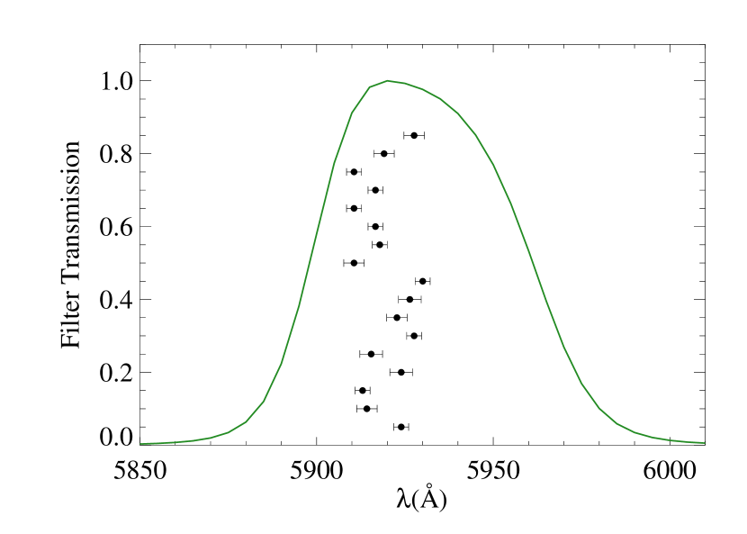
Figure 1.— Normalized NB filter transmission curve (green). Each point shows the wavelength in which the Ly$\alpha$ emission line of each quasar lie at their systemic redshift reported in Table  1. Y-axis position of the points is arbitrary. Quasar redshifts have been determined from the quasar SDSS/BOSS spectra by centroiding one or more of their rest-frame UV emission lines, SIV, CIV and CIII]. Then, we determined systemic redshifts by using the calibration of emission line shifts from Shen et al. (2007) (see details in § II.1). The Ly$\alpha$ emission line for all the quasars including their 1$\sigma$ errors lies in the central part of our NB filter.

Since radio loud quasars are known to reside in dense environments (e.g. Venemans et al., 2007), and are observed to cluster more strongly (e.g. Shen et al., 2009), we chose to focus our study on radio-quiet quasars. We thus discarded all quasars from our initial selection which had a radio emission counterpart at 20cm reported in the the Faint Images of the Radio Sky at Twenty-centimeters (FIRST; Becker et al., 1995) catalog. Finally, we also discarded quasars with high galactic extinctions ($A_{\lambda}>0.2$) toward their line of sight, and with close bright stars that could affect the imaging. A sample of 29 quasars satisfied all the mentioned criteria, and we selected the final sample of 17 quasars based on their visibility conditions and gave a higher priority to the brightest objects. A summary of the properties of the quasars we targeted is given in Table 1.

Table 1Targeted quasar properties.

Field	RA (J2000)	DEC (J2000)	Systemic Redshift	$i$
SDSSJ0040+1706	00:40:17.426	+17:06:19.78	3.873 $\pm$ 0.008	18.91
SDSSJ0042–1020	00:42:19.748	-10:20:09.53	3.865 $\pm$ 0.012	18.57
SDSSJ0047+0423	00:47:30.356	+04:23:04.73	3.864 $\pm$ 0.008	19.94
SDSSJ0119–0342	01:19:59.553	-03:42:16.51	3.873 $\pm$ 0.013	20.49
SDSSJ0149–0552	01:49:06.960	-05:52:18.85	3.866 $\pm$ 0.013	19.80
SDSSJ0202–0650	02:02:53.765	-06:50:44.54	3.876 $\pm$ 0.008	20.64
SDSSJ0240+0357	02:40:33.804	+03:57:01.59	3.872 $\pm$ 0.012	20.03
SDSSJ0850+0629	08:50:13.457	+06:29:46.91	3.875 $\pm$ 0.013	20.40
SDSSJ1026+0329	10:26:32.976	+03:29:50.63	3.878 $\pm$ 0.008	19.74
SDSSJ1044+0950	10:44:27.798	+09:50:47.98	3.862 $\pm$ 0.012	20.52
SDSSJ1138+1303	11:38:05.242	+13:03:32.61	3.868 $\pm$ 0.008	19.10
SDSSJ1205+0143	12:05:39.550	+01:43:56.52	3.867 $\pm$ 0.008	19.37
SDSSJ1211+1224	12:11:46.935	+12:24:19.08	3.862 $\pm$ 0.008	19.97
SDSSJ1224+0746	12:24:20.658	+07:46:56.33	3.867 $\pm$ 0.008	19.08
SDSSJ1258–0130	12:58:42.118	-01:30:22.75	3.862 $\pm$ 0.008	19.58
SDSSJ2250–0846	22:50:52.659	-08:46:00.22	3.869 $\pm$ 0.012	19.44
SDSSJ2350+0025	23:50:32.306	+00:25:17.23	3.876 $\pm$ 0.012	20.61

II.2. Imaging on 17 Quasar Fields

Imaging observations for the sample of 17 quasar fields were carried out using the FOcal Reducer and low dispersion Spectrograph 2 (FORS2, Appenzeller & Rupprecht 1992) instrument on the the Very Large Telescope (VLT) on 19 different nights between September, 2014 and March, 2015 (Program ID: 094.A-0900). The field-of-view of FORS2 is $6.8\times 6.8$ arcmin² corresponding to $\sim 9.8\times 9.8\,h^{-2}{\rm cMpc}^{2}$ at $z=3.88$. We used a $2\times 2$ binning readout mode, which results in an image pixel scale of $\rm 0.25\arcsec/pix$. Each quasar field was observed using the NB HeI ($\lambda_{\rm c}=5930$Å, $\rm FWHM=63$Å) and the broad bands $g_{\rm HIGH}~{}(\lambda_{\rm c}=4670$Å, hereafter $g$) and $R_{\rm SPECIAL}~{}(\lambda_{\rm c}=6550$Å, hereafter $R$) in order to detect LAEs at $z\sim 3.88$ (see top left panel of Fig. 5).

The total exposure time per target for HeI, $R$, and $g$ was 3660s, 360s, and 900s respectively, which were broken up into shorter individual exposures with dithering in order to fill the gap between the CCDs. Note that the full sequence of exposures for a given object were not necessarily observed on the same night. The seeing for the 19 nights cover a range of $0.6-1.5\arcsec$ and the median seeing is $0.94\arcsec$.

II.3. Data Reduction and Photometric Catalogs

We performed the data reduction using standard IRAF tasks and our own custom codes written in the Interactive Data Language (IDL). The reduction process included bias subtraction and flat fielding, which was performed based on twilight flats.

Given that individual science frames per field could have been observed in different nights, the photometric calibration was done before the final image stack was created. For the calibration of the $R$ images, Stetson photometric fields (Stetson, 2000) were observed in this band several times during the course of each night. We considered all the non-saturated photometric stars observed in the field and obtained their instrumental magnitude by using SExtractor (Bertin & Arnouts, 1996). Then, we computed the zeropoint by comparing these magnitudes with the tabulated standard star $R$ magnitudes from the Stetson catalogs, after correcting them with the corresponding color term to take into account the difference between the Stetson and FORS2 $R$ filter curves. The final zeropoint was computed as the median of the zeropoint obtained from each individual star of the field. The final zeropoint varies slightly over different nights ($<1\%$), and the uncertainties in the zeropoints are typically $0.02$ mag.

Spectrophotometric standard stars from different catalogs (Oke, 1990; Hamuy et al., 1992, 1994) were observed each night to calibrate the HeI and $g$ images. For each night, we computed the spectrophotometric star magnitude by convolving the HeI and $g$ filter transmission curve with the star spectra and then we compared this magnitude with the instrumental magnitudes obtained using SExtractor for the observed star in both HeI and $g$ bands. For 3/19 nights, no spectrophotometric standard star was observed in the $g$ band. For one of those nights, we had a Stetson photometric field observed in the $g$-band, which was then used to perform the flux calibration analogous to the $R$ image flux calibration. For the other two nights, we performed the flux calibration by using the SDSS photometric catalogs of stars in the science fields. Specifically, we compared the SDSS $g$ magnitudes of several stars in the field with their instrumental magnitude measured on our science images, and then we computed the zeropoint for those nights.

We calibrated all the individual science exposures using the computed zeropoints, and then we corrected them for extinction due to airmass using the atmospheric extinction curve for Cerro Paranal (Patat et al., 2011), and for galactic extinction calculated using Schlegel et al. (1998) dust maps and the Cardelli et al. (1989) extinction law with R${}_{V}=3.1$. We used SCAMP (Bertin, 2006) to compute the astrometric solution of each frame, using the SDSS-DR9 r-band catalogs as the astrometric reference. The typical RMS obtained in the astrometric calibration is $<0.15\arcsec$. Finally, the individual images were sky-subtracted, re-sampled and median-combined using SWarp (Bertin et al., 2002). The noisy edges of the combined images were trimmed out. Example reduced image in the HeI and $R$ filters is shown in Fig 2.

Figure 2.— HeI (left) and $R$ (right) reduced images of the SDSSJ0119–0342 field, centered on the quasar (red box). Detected LAEs are highlighted (red circles).

Object detection and photometry were performed using SExtractor in a dual mode. Since we are interested in the detection of objects with a strong Ly$\alpha$ emission line located in the core of our NB, we used the HeI image for the object detection. In order to perform an adequate measurement of the object colors, for each field we convolved our images with a Gaussian kernel to match the point-spread function (PSF) of the $R$, $g$ and HeI images such that their final PSF corresponds to the PSF of the image with the worst seeing. In Table 2 we indicate the seeing values for each field, measured after the convolution. We measured the object aperture magnitudes using a fixed aperture of $2\arcsec$ diameter. Objects not detected or detected with a signal-to-noise ratio (${\rm S/N})<2$ either in $g$ or $R$, were assigned the value of the corresponding $2\sigma$ limiting magnitude, listed in Table 2. Here, the ${\rm S/N}$ of each object is computed as the ratio of the aperture flux measured by SExtractor and the rms sky noise computed using our own IDL procedure, which performs $2\arcsec$ aperture photometry in $\sim 5000$ different random positions in the image to compute a robust measurement of the mean sky noise in each single aperture. The rms sky noise is then calculated as the standard deviation of the distribution of the $\sim 5000$ measured mean sky noise values. In Table 2 we listed the $2\sigma$ and $5\sigma$ limiting magnitude measured for each field. The median of the $5\sigma$ limiting magnitude for our fields is 24.45, 25.14 and 25.81 for the HeI, $R$ and $g$ images respectively.

Table 2$5\sigma$ and $2\sigma$ limiting magnitudes per field measured in a $2\arcsec$ diameter aperture. We also show the seeing measured on the HeI images and the seeing measured after matching the PSF of the images.

Field	HeI5σ	$R_{5\sigma}$	$g_{5\sigma}$	HeI2σ	$R_{2\sigma}$	$g_{2\sigma}$	seeing [$\arcsec$]	seeingFinal [$\arcsec$]
SDSSJ0040+1706	24.35	25.14	25.72	25.35	26.13	26.72	0.86	1.24
SDSSJ0042–1020	24.40	25.08	25.79	25.39	26.08	26.78	1.12	1.26
SDSSJ0047+0423	24.50	25.15	25.83	25.50	26.15	26.82	1.22	1.37
SDSSJ0119–0342	24.37	25.11	25.86	25.37	26.10	26.85	0.68	0.75
SDSSJ0149–0552	24.45	25.11	25.92	25.45	26.11	26.92	0.72	0.97
SDSSJ0202–0650	24.40	25.16	25.85	25.39	26.15	26.85	1.17	1.17
SDSSJ0240+0357	24.60	25.14	25.70	25.59	26.13	26.70	0.98	0.98
SDSSJ0850+0629	24.48	25.17	25.76	25.48	26.17	26.75	0.83	1.00
SDSSJ1026+0329	24.54	24.92	25.85	25.54	25.91	26.85	1.08	1.11
SDSSJ1044+0950	24.51	25.15	25.93	25.50	26.14	26.92	0.90	1.21
SDSSJ1138+1303	24.40	24.84	25.66	25.39	25.83	26.66	0.86	1.07
SDSSJ1205+0143	24.52	25.19	25.91	25.51	26.19	26.91	1.13	1.49
SDSSJ1211+1224	24.37	24.78	25.70	25.36	25.78	26.70	0.65	0.71
SDSSJ1224+0746	24.43	24.91	25.67	25.42	25.90	26.66	1.02	1.16
SDSSJ1258–0130	24.43	25.15	25.88	25.42	26.15	26.87	0.96	1.24
SDSSJ2250–0846	24.55	25.06	25.81	25.54	26.06	26.81	0.87	1.02
SDSSJ2350+0025	24.45	25.17	25.72	25.44	26.17	26.71	0.61	0.63

One way to check if the reduction process and flux calibration is correct for our NB filter is to compute the number counts from the HeI images and compare it with the $R$-band number counts measured by previous work. The central wavelength of the HeI filter ($\lambda_{\rm c}=5930$Å) is sufficiently close to the central wavelength of the $R$-band filter ($\lambda_{\rm c}=6550$Å), such that for sources whose spectra do not vary strongly across the extend of the $R$-band filter, the HeI magnitude is a good proxy for the $R$ magnitude. Thus we expect that the HeI number counts should be a decent proxy for the $R$-band number counts measured previously. For this check, we used a compilation of $R$-band number counts measured in 0.5 mag bins that includes number counts measured in the SDSS r-band as well as those measured in the $R$ Kron-Cousins band (Metcalfe et al., 2001; Shanks et al., 2015). We compared this with the number counts detected in all our fields in 0.5 mag bins divided by the total effective area of our survey. We show our results in Fig. 3, and we see that the HeI number counts agree fairly well with the $R$-band number counts. The disagreement at the faintest magnitudes we probe is due to incompleteness in the detection of sources in our images.

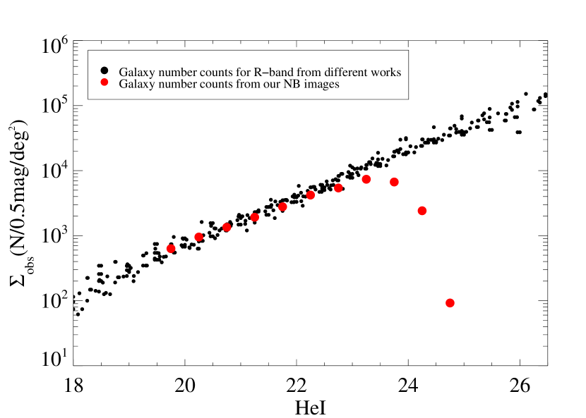
Figure 3.— HeI number counts detected in our NB images (red points) compared with the $R$-band number counts measured in previous studies (black points). In our NB images we find similar number counts as those detected in the $R$-band in previous studies, which validates the reduction process and flux calibration performed for the HeI filter.

We directly measured the completeness in the object detection in our HeI images for each field as follows. Artificial point-sources with a fixed total magnitude were inserted at random locations into the HeI images and then we ran SExtractor on these new images including artificial sources in the same way we did to create our photometric catalogs. The completeness per field was computed as the fraction of artificial sources that were actually detected. We repeated this procedure for different magnitudes bins spaced by 0.1. We computed the median of the completeness over our fields which is shown in Fig. 4. Note that the object completeness depends on the size of the object, thus our completeness computation is only valid for LAEs at $z\sim 4$ which are assumed to be unresolved in our images (the typical effective radius of $z\sim 4$ LAEs is $r_{e}\sim 0.5$  pkpc (e.g. Shibuya et al., 2019) which corresponds to $0.07\arcsec$ at $z=4$).

Figure 4.— Median of the completeness in the object detection on the HeI images as a function of the HeI magnitude. This completeness is computed for point sources.

III. LAE Number Density in Quasar Fields

In this section we describe how LAEs were selected, we present the sample, and we compute the LAE number density in our fields to compare with the number counts in blank fields.

III.1. LAE Selection Criteria

As we discuss in the next section, clustering measurements are based on the comparison of the LAE number density detected in our fields to that expected at random locations in the universe. This last quantity should be preferentially computed either from blank fields observed using the same filter configuration as our quasar fields or from the outer parts of the images when the field-of-view is large enough such that the background level is reached. Given that we do not have control fields and that the field-of-view of FORS2 is not large enough for a determination of this background, the only alternative is to compute it from which the $z\sim 4$ LAE luminosity function measured in previous studies. This may introduce systematic errors if our procedure for selecting LAEs differs from that used in previous work on blank fields from which the LAE luminosity function has been estimated. In order to limit the impact of such systematics and thus enable a robust clustering measurement, we must be careful to select our LAEs following the same criteria adopted by previous studies.

Here we use the LAE luminosity function measured by Ouchi et al. (2008), who selected $z=3.69$ LAEs using Subaru Suprime-Cam imaging data obtained in the filters $B$, $\rm NB570$ and $V$ analogously to our filter configuration $g$, HeI, and $R$ (see top right panel of Fig. 5). The LAE color selection criteria they used are defined by the equations $V-{\rm NB570}>1.3$ and $B-V>0.7$, thus we need to translate their color cuts to our $R-{\rm HeI}$ and $g-R$ colors respectively. If we perform our LAE selection exactly as they do, then we can ensure that the color completeness (i.e the completeness of the LAEs selection which does not have to be confused with the photometric completeness computed in  § II.3), contamination level, and the underlying background number density of our LAE sample is the same as theirs.

The $V-{\rm NB570}$ color provides information about the observed-frame Ly$\alpha$ equivalent width (EW_Lyα) of the selected galaxy. Thus we must compute the limiting ${\rm EW}_{\rm Ly\alpha}$ value which corresponds to the Ouchi et al. (2008) color cut $V-{\rm NB570}>1.3$, and choose a color cut using our filters that isolates LAEs of the same ${\rm EW}_{\rm Ly\alpha}$. The observed-frame ${\rm EW}_{\rm Ly\alpha}$ is defined as:

$${\rm EW}_{\rm Ly\alpha}=\int\frac{F_{\rm Ly\alpha}}{F_{\rm cont,Ly\alpha}}d\lambda,$$ (1)

where $F_{\rm Ly\alpha}$ is the specific flux of the ${\rm Ly\alpha}$ line (with the continuum subtracted), and $F_{\rm cont,Ly\alpha}$ is the specific flux of the continuum at the wavelength of the ${\rm Ly\alpha}$ line. The flux in the NB570 and the $V$ filters provides information about the flux of the ${\rm Ly\alpha}$ line plus the continuum covered by each filter curve, respectively. Note that the shape of the continuum over the NB570 and $V$ bands is not trivial, because there is a flux break at $\lambda_{\rm rest-frame}=1216$Å  due to the absorption of photons with $\lambda_{\rm rest-frame}<1216$Å  by neutral hydrogen in the intergalactic medium (see for example the LAE simulated spectra in the top-panels of Fig. 5). This makes it challenging to analytically compute both $F_{\rm Ly\alpha}$ and $F_{\rm cont,Ly\alpha}$ only from a $V-{\rm NB570}$ color information (the same complication applies to using our $R$ and HeI filters to select LAEs at $z=3.88$). Our approach to determine the EW_Lyα from color measurements and determine the equivalent set of color selection criteria in our filter is to simulate LAE spectra with different EW_Lyα values, and then integrate them against the filters $V$ and NB570 to compute the colors from the simulated galaxy spectra. Once we determine which set of model galaxy parameters reproduce the $V-{\rm NB570}$ color value used by Ouchi et al. (2008), we integrate the same spectra (now with known EW_Lyα) against our filters $R$ and HeI, and we define the $R-{\rm HeI}$ color criteria that we should use.

To simulate the LAE spectra, we start with a template star-forming galaxy spectrum generated from a Bruzual & Charlot (2003) stellar population synthesis model, corresponding to an instantaneous burst of star-formation with an age of 70Myr, a Chabrier (2003) IMF, and a metallicity of 0.4Z_⊙. We measured the UV slope of this template over the range 1300Å$<\lambda<$2000Å  by fitting a power law shape given by $A\lambda^{\alpha}$, and then we modify its UV slope by multiplying by the power law required to obtain a final flat UV continuum ($\propto\lambda^{-2}$), which is expected for LAEs at $z\sim 4$ (Overzier et al., 2008; Ouchi et al., 2008). We then multiplied the resulting spectrum at $\lambda\leq 912$Å  by an escape fraction parameter $f_{\rm esc}^{\lambda<912}=0.05$ to take into account the fact that only a small fraction of Lyman limit photons are able to escape high-redshift galaxies. To simulated the Ly$\alpha$ emission, we added Gaussian line with rest-frame central wavelength $\lambda_{\rm Ly\alpha}=1215.7$Å, a $\rm FWHM_{\rm Ly\alpha}=1.05$Å  (or equivalently $\rm 260\,km\,s^{-1}$) which agrees with measurements for high-redshift LAEs (e.g. Venemans et al., 2005; Shimasaku et al., 2006), and amplitude $B$ which adjusts the intensity of the line in order to model a Ly$\alpha$ line with a chosen rest-frame EW_Lyα computed using eqn. (1). Finally, we redshifted the spectra to $z=3.69$ (i.e., we are assuming that the line is in the center of the NB filter) and attenuate the flux blueward of the ${\rm Ly\alpha}$ line using an IGM transmission model $T_{z}(\lambda)$ from Worseck & Prochaska (2011), which models the foreground Lyman series absorption from the IGM. Note that we only attenuate the continuum flux, but we do not attenuate the flux of the ${\rm Ly\alpha}$ line. In this way, the chosen rest-frame EW_Lyα value in our simulation correspond to an apparent EW_Lyα, which is assumed to be already affected by the IGM absorption, and then this is comparable to the EW_Lyα values measured directly from observed LAEs. This is different from the intrinsic EW_Lyα which is the EW_Lyα after corrected for the effect of foreground IGM absorption. We simulate spectra with different rest-frame EW_Lyα values and integrated them against the filters used by Ouchi et al. (2008) to compute $V-{\rm NB570}$. We find that a LAE with rest-frame EW${}_{\rm Ly\alpha}=28$Å  reproduces the color criteria used by Ouchi et al. (2008) of $V-{\rm NB570}=1.3$. We then redshifted such spectra up to $z=3.88$ (using the corresponding redshift dependent IGM transmission model) and integrated it against our filters, finding $R-{\rm HeI}=0.98$, which defines the color criteria to select LAEs using our filter configuration.

We show an example of a simulated spectra at $z=3.88$ in the top left panel of Fig. 5. We also used our simulated spectra to compute an evolutionary track of LAEs in the color-color diagram. To this end, we redshifted it from $z=3.2$ to $z=4.4$ with a spacing of 0.02, applied the corresponding IGM transmission model in each redshift step, and integrated the spectrum against both our and Ouchi et al. (2008) filter curves. The evolutionary tracks are shown in the bottom left panel of Fig. 5 for the $g$, HeI, $R$ filter set and in the bottom right panel of Fig. 5 for the $B$, $\rm NB570$ and $V$ filter set.

Figure 5.— Top left: Filter transmission curves used in this work shown on a simulated LAE spectra redshifted to $z\sim 3.88$. The simulated spectra correspond to a galaxy with a flat UV continuum slope ($\propto\lambda^{-2}$) and with a $\rm Ly\alpha$ equivalent width of $28$Å  (in rest-frame). Bottom left: Evolutionary track of a LAE with EW${}_{\rm Ly\alpha}=28$Å  (black curve). Filled circles over the black curve indicate colors of LAEs from redshift 3.3 to 4.0, and the large red point indicate the exact position of the color of a LAE at $z=3.88$. For comparison, we also plotted the evolutionary track of a LAE with EW${}_{\rm Ly\alpha}=100$Å  (gray curve). We overplotted the evolutionary tracks of other galaxies for our filter system redshifted from $z=0$ to $z=3$. We plot as brown, magenta, orange, blue, and red curves the evolutionary track of elliptical, Sa, Sb, Sc, and irregular galaxies respectively. The black dashed line show the selection region used in this work to select LAEs. Top right: Filter transmission curves used in Ouchi et al. (2008) shown on the simulated LAE spectra redshifted to $z\sim 3.69$. Bottom right: Same as the bottom left panel, but for the Ouchi et al. (2008) filter system. In this case the large red point over the black curve indicate the exact position of the color of a LAE at $z=3.69$. The black dashed line show the selection region used by Ouchi et al. (2008) to select LAEs.

The second color criteria used by Ouchi et al. (2008) to select LAEs is $B-V>0.7$, which guarantees a low level of low-redshift galaxy contamination in the resulting sample (they estimate a contamination level of $0-14\%$). We studied the $B-V$ colors of typical LAEs by using our simulated spectra with EW${}_{\rm Ly\alpha}=28$Å. We modified the UV continuum slope of the spectra in order to span the range of observed values in $z=4$ galaxies which goes from $\alpha=-3$ to $\alpha=0$ (Bouwens et al., 2009), and we found that in this range the $B-V$ color varies from $1.7$ to $2.2$. Given our parametrization of the escape fraction and the IGM absorption, a simulated LAE would have a color of $B-V=0.7$ only if their spectra had an UV continuum slope of $\alpha=-8.8$, which is unphysically steep. Therefore, typical LAEs always satisfy the $B-V$ condition, and it is chosen mostly to exclude low-redshift galaxy contamination.

We study the colors of low-redshift galaxies in both the $B$, $V$ and the $g$, $R$ filter system in order to compare how different they are. We used a set of five galaxy templates, typically used to estimate photometric redshifts. The templates are from the photo-$z$ code EASY (Brammer et al., 2008), which are distilled from the PEGASE spectral synthesis models. We redshifted these templates from $z=0$ to $z=3$, and integrated them against the $B$, NB570, $V$, and the $g$, HeI, $R$ filter transmission curves to generate their evolutionary track in the color-color diagram. We show our results in the bottom panels of Fig. 5. Given that low-redshift galaxies have similar $B-V$ and $g-R$ colors, we simply adopt the same color cut as in Ouchi et al. (2008) for our filters, given by $g-R>0.7$. The locus of the low-redshift galaxies is well isolated from the location of the LAEs we wish to select, and the $g-R=0.7$ color cut helps exclude strong OIII emitters at $z=0.18$ or OII emitters at $z=0.59$, represented by the two peaks in the green curves in the bottom panels of Fig. 5.

To summarize, the color cuts used in this work are thus:

$$R-{\rm HeI} >0.98$$ (2)

$$g-R >0.7$$

III.2. LAE Sample

We used our photometric catalogs to select LAE candidates in our 17 quasar fields. In order to ensure a solid detection in the NB filter, we only selected objects detected with ${\rm S/N}\geq 5.0$ in the HeI band. We required that sources have the SExtractor parameter $\rm FLAGS=0$ in order to exclude blended, saturated or truncated sources. Additionally, we created masks from our images to indicate “bad regions”, which are defined as regions where the object detection is not reliable. Some examples of such regions are locations in the vicinity of extremely bright stars (since contamination from bright objects affect the photometry of nearby sources), highly extended objects which cover a large area of the image (which may preclude the detection of background LAEs), and satellite trails. We discarded all the sources located on the defined bad regions. Note that these masks are also used in the clustering analysis presented in section  § IV to compute the effective area of our survey. All the objects in our 17 quasar fields satisfying the aforementioned requirements are plotted in the color-color diagram shown in Fig. 6.

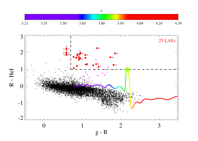
Figure 6.— Color-color diagram for our 17 stacked quasar fields. Here the LAE evolutionary track showed in the bottom left panel of Fig. 5 is plotted as redshift color-coded track according to the color bar. Magenta points indicate the color of the quasar in our filters. Arrows indicate lower limits for the colors, and then double arrows represent cases in which the object was not detected at 2$\sigma$ level in either $g$ and $R$ images, and each magnitude was replaced by the corresponding limit magnitude. The dashed line is indicating the selection region defined by eqns. (2). We have highlighted the selected LAEs of our main sample as red points.

All the objects satisfying the color criteria in eqns. (2) were selected as LAEs (this selection region is shown as a dashed line in Fig. 6). We discarded objects with $\rm HeI<22.7$ in order to exclude bright low-redshift interloper galaxies that might be affecting our selection. This lower limit is the same used by Ouchi et al. (2008). Note that data points with double arrows in the x-axis of this figure represent cases in which the object was not detected at the 2$\sigma$ level in either $g$ and $R$ images, and each magnitude was replaced by the corresponding limiting magnitude in each field. Thus the position on the g-R axis of these points is determined by the depth of our $g$ and $R$ images, but does not provide any actual information about the $g-R$ color. We note that the broad band limiting magnitude of the Ouchi et al. (2008) work are deeper than ours (their $V$ images are $\sim$2.0 mag deeper than our corresponding depth in $R$, and $B$ images are $\sim$1.8 mag deeper than our $g$ depth). If we had deeper $R$ images left pointing arrows would move to the left and upward pointing arrows would move up in Fig. 6, then we could lose some of the selected LAEs, but we would not gain objects. On the other hand, deeper $g$ images would move right pointing arrows to the right, and we could only gain objects. Specifically there are three additional objects that could satisfy the color criteria (the objects with double arrows in the $g$-$R$ direction outside of our selection region in Fig. 6), and for this reason, we also considered them as LAEs. We recall that the $g-R>0.7$ color cut is chosen mostly to mitigate low-redshift interlopers, and for such interlopers we expect a solid detection in both $g$ and $R$ at the 2$\sigma$ limiting magnitude of our observations. The fact that these three additional objects are not detected in our broad bands suggests that are more likely to be LAEs. Our final sample, comprises 25 LAEs whose photometry is shown in Table 3. We show cutout images of the detected LAEs in Fig. 7. We also show the distribution of LAEs around the central quasar for all the fields together in Fig. 8.

Table 3Properties of LAE candidates. The magnitudes correspond to AB magnitudes measured in a $2\arcsec$ diameter aperture for each band.

ID	RA	DEC	$R$	$g$	HeI
	(J2000)	(J2000)
SDSSJ0040$+$1706_1	10.04149	17.10328	25.27	26.55	24.04
SDSSJ0040$+$1706_2	10.03181	17.07825	25.80	$>$26.72	24.21
SDSSJ0040$+$1706_3	10.01593	17.09058	$>$26.13	$>$26.72	24.29
SDSSJ0119$-$0342_1	20.00311	-3.65073	25.99	$>$26.85	24.15
SDSSJ0119$-$0342_2	20.00470	-3.65074	25.78	$>$26.85	23.94
SDSSJ0119$-$0342_3	19.99616	-3.70381	25.47	$>$26.85	23.23
SDSSJ0119$-$0342_4	20.00119	-3.67776	25.61	26.39	23.90
SDSSJ0119$-$0342_5	20.03121	-3.67618	25.00	$>$26.85	23.08
SDSSJ0240$+$0357_1	40.09660	3.92959	25.61	26.46	23.96
SDSSJ0850$+$0629_1	132.57429	6.44336	25.39	$>$26.75	24.09
SDSSJ0850$+$0629_2	132.57962	6.46084	$>$26.17	$>$26.75	23.98
SDSSJ0850$+$0629_3	132.52617	6.52619	$>$26.17	$>$26.75	24.20
SDSSJ1026$+$0329_1	156.67078	3.48840	$>$25.91	$>$26.85	24.00
SDSSJ1026$+$0329_2	156.58314	3.52040	25.03	$>$26.85	23.79
SDSSJ1044$+$0950_1	161.07159	9.83493	25.74	26.69	23.80
SDSSJ1205$+$0143_1	181.42337	1.69562	25.03	26.45	23.90
SDSSJ1211$+$1224_1	182.93760	12.41883	25.61	26.56	23.97
SDSSJ1211$+$1224_2	182.89731	12.41925	24.97	$>$26.70	23.27
SDSSJ1211$+$1224_3	182.88843	12.39337	25.30	26.16	24.11
SDSSJ1211$+$1224_4	182.95711	12.39097	$>$25.78	26.68	24.07
SDSSJ1211$+$1224_5	182.92907	12.43754	24.77	25.55	23.71
SDSSJ1211$+$1224_6	182.90785	12.43242	25.46	26.37	23.90
SDSSJ1258$-$0130_1	194.71644	-1.48276	25.34	26.42	23.68
SDSSJ2250$-$0846_1	342.72901	-8.71839	25.13	26.22	23.87
SDSSJ2350$+$0025_1	357.62878	0.46156	24.84	25.96	23.54

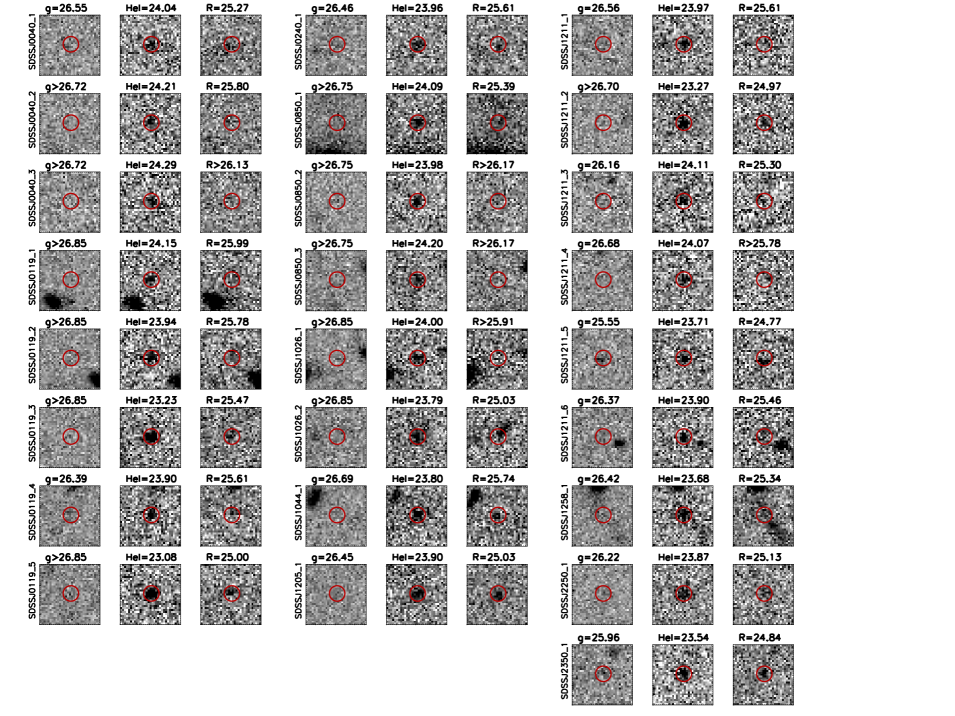
Figure 7.— $g$, HeI, and $R$ images of all the LAE sample, exhibited in panels of $7.5\arcsec\times 7.5\arcsec$. A red circle of $2\arcsec$ in diameter shows the position of the detected LAEs. Magnitudes are indicated in each panel.

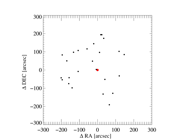
Figure 8.— Distribution of the 25 LAEs with respect to the central quasar plotted as a red dot.

III.3. Comparison with the Number Density of LAEs in Blank Fields

Here we compute the total number density of LAEs in our quasar fields and compare it with the LAE number density measured in blank fields. Given that we matched the LAE selection criteria with that used in Ouchi et al. (2008), we directly compare our number density with theirs.

We compute the number density of LAEs, by dividing the number of observed LAEs per HeI magnitude bin by the effective survey volume. For the computation of the effective survey volume, we assumed a top-hat function for our NB filter curve transmission function, with width equal to the FWHM (63Å), and computed the comoving distance coverage at $z=3.88$, resulting 37.4 cMpc. We multiply this quantity by the effective area of our survey, which is computed per field by subtracting the masked area from the total area of the image. The total area of our survey is obtained by adding the effective area of the 17 fields (listed in Table 4). We obtain that our survey covered a total area of 740.8 arcmin² corresponding to 3,146 cMpc². We compared our measurement with the results from Ouchi et al. (2008) in Fig. 9 (we have converted the surface number counts presented in Ouchi et al. (2008) to the volume number counts by taking into account the FWHM of their NB filter transmission curve (69Å), which corresponds to a comoving distance coverage of 43.2 cMpc at $z=3.7$).

Note that all our quasar fields reach different NB limiting magnitude (with a median $5\sigma$ limiting magnitude of $24.45$) and have different object completeness detection. We have also computed the completeness-corrected number density by using the completeness we determined per field as described in § II.3 which is shown in Fig. 9. We recall that the HeI magnitude is not providing information about the Ly$\alpha$ line flux, but rather about the sum of the Ly$\alpha$ line flux and the continuum flux. We find that the number density of LAEs in quasar fields is consistent with that measured in blank fields for the brightest NB magnitudes bins but we detected a significantly higher number density (by a factor of 3.1) for LAEs with $23.7<NB<24.2$, the range in which most of our objects (18 out of 25) are. We find agreement with the Ouchi et al. (2008) number density for the faintest magnitude bin, which only contains 2 of our LAEs, but we note that our sample is highly incomplete at those magnitudes (completeness of $\sim$10%, as shown in Fig. 4), thus our completeness-corrected number density could be dominated by errors in the completeness computation in this magnitude range. Overall, our results suggest that we have detected an overdensity of LAEs in quasar environments on the scales probed by this work ($R\lesssim 7\,h^{-1}\,{\rm cMpc}$).

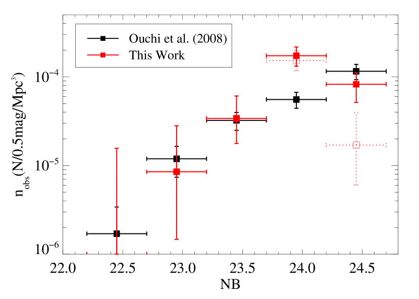
Figure 9.— LAEs number density for our 17 stacked fields. The black squares are the LAEs number density per NB570 magnitude range in blank fields (Ouchi et al., 2008), the filled red squares are the completeness-corrected LAEs number density per HeI magnitude range in quasar fields computed using our LAE sample, with error bars computed using one-sided Poisson confidence intervals for small number statistics from Gehrels (1986). Open red squares are this measurement before to consider the completeness detection. We detect an overdensity of LAEs in quasar fields compared with that measured in blank fields.

IV. Clustering Measurements

In the last section we showed that quasar fields have a higher number density of LAEs than blank field pointings. By measuring the cross-correlation and auto-correlation function of LAEs in our survey, we can further quantify the clustering of LAEs around quasars and determine their spatial profile. To measure the clustering of LAEs in quasar fields, we perform the same analysis presented in García-Vergara et al. (2017). Here we only describe the most important points and refer the reader to that paper for further details.

IV.1. Quasar-LAE Cross-correlation Function

We measure a volume-averaged projected cross-correlation function between quasars and LAEs defined by

$$\chi(R_{\rm min},R_{\rm max})=\frac{\int\xi_{QG}(R,Z)dV_{\rm eff}}{V_{\rm eff}},$$ (3)

where $\xi_{QG}(R,Z)$ is the real space quasar-LAE cross-correlation function and $V_{\rm eff}$ is the effective volume of the survey, defined as a cylindrical volume with transverse separation from $R_{\rm min}$ to $R_{\rm max}$ and height $Z$ which is the radial comoving width probed by our survey. We measured the volume-averaged projected cross-correlation function in logarithmically spaced radial bins centered on the quasar by using the estimator,

$$\chi(R_{\rm min},R_{\rm max})=\frac{\langle QG\rangle}{\langle QR\rangle}-1$$ (4)

where $\langle QG\rangle$ is the number of quasar-LAE pairs in the bin, which is directly measured by counting the quasar-LAE pairs found in our images, and $\langle QR\rangle$ is the expected number of quasar-LAE pairs in the same bin if they were randomly distributed around the quasar, with the background number density. The quantity $\langle QR\rangle$ is computed from:

$$\langle QR\rangle=n_{\rm G}(z,{L_{\rm Ly\alpha}>L_{\rm Ly\alpha}^{\rm limit}})V_{\rm eff},$$ (5)

where $n_{\rm G}(z,{L_{\rm Ly\alpha}>L_{\rm Ly\alpha}^{\rm limit}})$ is the mean number density of LAEs at redshift $z$ with $\rm Ly\alpha$ luminosity greater than the limiting $\rm Ly\alpha$ luminosity reached in our survey. Here, we use the LAE luminosity function measured by Ouchi et al. (2008) at $z=3.7$, which is given by the Schechter parameters $\phi^{*}=3.4\times 10^{-4}$ Mpc^-3, $L^{*}_{\rm Ly\alpha}=1.2\times 10^{43}$ erg s^-1 mag, and $\alpha=-1.5$. We compute $n_{\rm G}(z,{L_{\rm Ly\alpha}>L_{\rm Ly\alpha}^{\rm limit}})$ for each individual quasar field by integrating the luminosity function up to the 5$\sigma$ limiting $\rm Ly\alpha$ luminosity of the field in question. Note that converting from the 5$\sigma$ limiting HeI magnitude (presented in section § II.3) to the 5$\sigma$ limiting $\rm Ly\alpha$ luminosity is not trivial because the HeI magnitude includes both the flux of the $\rm Ly\alpha$ line and the flux of the continuum. For this conversion, we have used our simulated LAE spectra (created as we describe in section § III.1) to compute the $\rm Ly\alpha$ limiting luminosity corresponding to a given HeI limiting magnitude. Specifically, we simulate a flat UV continuum LAE spectrum ($\propto\lambda^{-2}$) with both a fixed $\rm EW_{Ly\alpha}=28$Å  and without the $\rm Ly\alpha$ emission line. Then, we determine the flux that both spectra would have in the HeI filter, and then subtract them to obtain the $\rm Ly\alpha$ luminosity. In other words, the resulting $\rm Ly\alpha$ luminosity depends on the assumed $\rm EW_{Ly\alpha}$ value, and the properties of the simulated spectrum. We choose the $\rm EW_{Ly\alpha}$ value here to match the limiting equivalent width of our LAE selection. Considering our limit $\rm EW_{Ly\alpha}=28$Å  the $\rm Ly\alpha$ luminosity could be sightly underestimated if the candidates typically have greater $\rm EW_{Ly\alpha}$ values (specifically, if we consider LAEs with $EW_{Ly\alpha}=80$Å  the $\rm Ly\alpha$ luminosity would change in a $\sim 8\%$), however, the errors associated with the Schechter parameters of the LAE luminosity function dominate over this relatively small source of error in the LAE number density computation. The mean 5$\sigma$ limiting $\rm Ly\alpha$ luminosity computed for our fields is listed in Table 4, on average we obtained $L_{\rm Ly\alpha}=4.1\times 10^{42}$ erg s^-1. Given that the source detection in our images is not 100% complete up to the 5$\sigma$ limiting $\rm Ly\alpha$ luminosity (see section § II.3), we have included the completeness correction in the computation of $n_{\rm G}(z,{L_{\rm Ly\alpha}>L_{\rm Ly\alpha}^{\rm limit}})$ by weighting the luminosity function by the source detection completeness computed as explained in section § II.3 for each field. We listed the $n_{\rm G}(z,{L_{\rm Ly\alpha}>L_{\rm Ly\alpha}^{\rm limit}})$ values per field in Table 4.

For the computation of the $V_{\rm eff}$ value in eqn. (5), we considered the volume of the bin defined by a cylinder with radial width $(R_{\rm max}-R_{\rm min})$ and height $Z$ which is computed from the FWHM of our NB filter (we approximate the filter curve transmission function as a top-hat function with a width equal to the FWHM). Specifically, for HeI, the $\rm FWHM=63$Å  corresponds to a redshift coverage of $\Delta z=0.052$ at $z=3.88$ (or equivalently $\rm 3,197\,km\,s^{-1}$) and a comoving distance of $Z=26.2\,h^{-1}$ cMpc. We also considered an angular selection function in this computation, which is estimated using the detection masks created from our images (see section § III.2). These masks quantify the fraction of the bin area where the LAEs were detectable. In Table 4 we show the effective volume of each field $V_{\rm field}$ (i.e the sum of the $V_{\rm eff}$ over the radial bins). We obtained that the total volume of our survey is 40,254 $\,h^{-3}$ cMpc³.

Table 4LAE number counts in each individual quasar field.

Field	$A_{\rm field}$	${\rm log}(L_{\rm Ly\alpha}^{\rm limit})$	$n_{\rm G}$	$V_{\rm field}$	$\langle QR\rangle_{\rm field}$	$\langle QG\rangle_{\rm field}$	$\delta$
(1)	(2)	(3)	(4)	(5)	(6)	(7)	(8)
SDSSJ0040$+$1706	42.56	42.65	0.49	2310.95	1.13	3	2.66
SDSSJ0042$-$1020	44.31	42.64	0.25	2407.74	0.60	0	0.00
SDSSJ0047$+$0423	45.05	42.59	0.25	2446.96	0.60	0	0.00
SDSSJ0119$-$0342	44.72	42.64	0.60	2430.48	1.46	5	3.41
SDSSJ0149$-$0552	44.42	42.61	0.64	2415.15	1.54	0	0.00
SDSSJ0202$-$0650	41.44	42.64	0.21	2255.96	0.47	0	0.00
SDSSJ0240$+$0357	44.48	42.56	0.45	2416.79	1.08	1	0.92
SDSSJ0850$+$0629	41.06	42.60	0.56	2235.92	1.25	3	2.41
SDSSJ1026$+$0329	45.04	42.58	0.38	2444.89	0.93	2	2.16
SDSSJ1044$+$0950	45.01	42.59	0.52	2444.62	1.28	1	0.78
SDSSJ1138$+$1303	37.68	42.64	0.45	2047.16	0.92	0	0.00
SDSSJ1205$+$0143	43.37	42.59	0.32	2356.25	0.75	1	1.34
SDSSJ1211$+$1224	45.05	42.64	0.65	2446.81	1.60	6	3.75
SDSSJ1224$+$0746	44.34	42.62	0.35	2410.69	0.84	0	0.00
SDSSJ1258$-$0130	44.12	42.62	0.39	2396.02	0.93	1	1.08
SDSSJ2250$-$0846	44.82	42.58	0.53	2434.21	1.30	1	0.77
SDSSJ2350$+$0025	43.32	42.61	0.72	2353.88	1.69	1	0.59
All	740.81			40254.46	18.36	25	1.36

Note. — (1) Field ID, (2) Total area of the field in units of arcmin², (3) 5$\sigma$ limiting $\rm Ly\alpha$ luminosity in units of log$($ erg s${}^{-1})$, (4) The mean number density of $z\sim 4$ LAEs in units of $(10^{-3}\,h^{3}$ cMpc${}^{-3})$, for $L_{\rm Ly\alpha}>L_{\rm Ly\alpha}^{\rm limit}$. Given that $L_{\rm Ly\alpha}^{\rm limit}$ and the source detection completeness are different for each field, we obtain a number density slightly different for each one, (5) Total volume of the field in units of $(h^{-3}$ cMpc${}^{3})$, (6) Total number of expected LAEs on the whole field. This is computed as $\langle QR\rangle_{\rm field}=n_{\rm G}V_{\rm field}$, (7) Total number of observed LAEs on the whole field, (8) Total overdensity per field, computed as $\langle QG\rangle_{\rm field}/\langle QR\rangle_{\rm field}$

In Table 4 we also list the values of $\langle QG\rangle_{\rm field}$ and $\langle QR\rangle_{\rm field}$ which correspond to the sum of the $\langle QG\rangle$ and $\langle QR\rangle$ values respectively over the bins for each individual quasar field. This provides a measurement of the individual overdensity $\delta=\langle QG\rangle_{\rm field}/\langle QR\rangle_{\rm field}$. We find that 7 out of 17 fields have more LAEs than the expected number in blank fields (i.e $\delta>1.0$). If we sum over all the $\langle QR\rangle_{\rm field}$ values for our 17 fields we obtain that one would expect to detect a total of $\sim 18.36$ LAEs for blank field pointings, whereas we detected a total of 25 LAEs, meaning that on average $z\sim 4$ quasars fields are overdense in LAEs by a factor of $\sim 1.4$.

We emphasize the fact that our conclusions are based on the average number density of 17 quasar fields. We note that 10 of our fields are indeed underdense, but they are not representative of the aggregate behavior of the quasars in our sample. Those 10 fields serve as a reminder of the large cosmic variance inherent in quasar environment studies, and the danger of over-interpreting noisy measurements made from studies where only a single quasar or a handful of fields are analyzed at the highest ($z\gtrsim 6$) redshifts.

We measure the quasar-LAE cross-correlation function by adding up the $\langle QG\rangle$ and $\langle QR\rangle$ values, computed in bins of transverse distance, for the 17 quasar fields and plugging those values into eqn. (4). We show our results in Fig. 10 and tabulate the values in Table 5. Given the small size of our LAE sample, we have assumed that Poisson error dominates our measurement, and in Fig. 10 we have plotted the one-sided Poisson confidence interval for small number statistics from Gehrels (1986). Notwithstanding the large errors, we do detect a positive quasar-LAE cross-correlation function which is consistent with a power-law shape indicative of a concentration of LAEs centered on the quasars.

Table 5quasar-LAE Cross-Correlation Function.

$R_{\rm min}$	$R_{\rm max}$	$\langle QG\rangle$	$\langle QR\rangle$	$\chi(R_{\rm min},R_{\rm max})$	$V_{\rm eff,total}$
$(h^{-1}$ cMpc)	$(h^{-1}$ cMpc)				$(h^{-3}$ cMpc${}^{3})$
0.178	0.368	1	0.068	13.719${}^{+33.854}_{-12.173}$	149.06
0.368	0.759	0	0.287	-1.000${}^{+6.408}_{-0.000}$	628.82
0.759	1.566	2	1.213	0.649${}^{+2.175}_{-1.065}$	2656.29
1.566	3.231	4	5.126	-0.220${}^{+0.617}_{-0.373}$	11237.91
3.231	6.664	18	11.645	0.546${}^{+0.457}_{-0.361}$	25538.90

Note. — Volume-averaged projected cross-correlation function between quasars and LAEs $\chi(R_{\rm min},R_{\rm max})$ defined according to eqn. (4) and measured in radial bins defined by $R_{\rm min}$ and $R_{\rm max}$ for our 17 stacked fields. We show the observed number of quasar-LAE pairs per bin $\langle QG\rangle$ and the expected number of quasar-random pairs per bin $\langle QR\rangle$ computed according to eqn. (5). The total volume of the bin added over the fields is also listed.

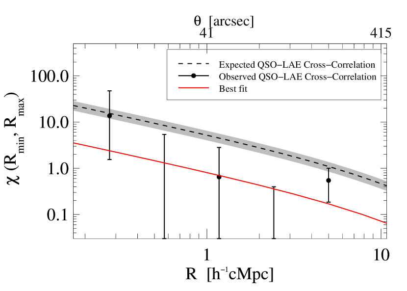
Figure 10.— Quasar-LAE cross-correlation function. The filled circles are showing our measurement with $1\sigma$ Poisson error bars and the red curve shows the best fit for our measurement given by $r^{QG}_{0}=2.78^{+1.16}_{-1.05}\,h^{-1}\,{\rm cMpc}$ for a fixed slope at $\gamma=1.8$. The dashed black line shows the theoretical expectation of $\chi$ for our 17 stacked fields computed from the quasar and LAEs auto-correlation functions and assuming a deterministic bias model. The gray shaded region indicates the $1\sigma$ error on the theoretical expectation computed by error propagation and based on the reported $1\sigma$ errors of the $r^{QQ}_{0}$ and $r^{GG}_{0}$ parameters.

In order to determine the real-space cross-correlation parameters $r_{0}^{QG}$ and $\gamma$ that best fit our data, we use a maximum likelihood estimator assuming a Poisson distribution for the number counts and fit following the same procedure described in García-Vergara et al. (2017). Given the large errors in our measurements, we fix the slope at $\gamma=1.8$ and find that the maximum likelihood and the $1\sigma$ confidence interval for the correlation length is $r^{QG}_{0}=2.78^{+1.16}_{-1.05}\,h^{-1}\,{\rm cMpc}$. We used this value in eqn. (3) to compute the corresponding $\chi(R_{\rm min},R_{\rm max})$ value which is shown as the red line in Fig. 10. In order to verify that our results are not sensitive to our chosen binning, we have also measured the cross-correlation function by changing the binning and again fitting, and we find that different binning choices only change the constrained $r^{QG}_{0}$ parameter within the uncertainties quoted above.

For comparison we have computed the expected value for the quasar-LAE cross-correlation function assuming a deterministic bias model. In other words, if $\delta_{G}$ and $\delta_{Q}$ are the density contrast of galaxies and quasars respectively, the cross-correlation between quasars and LAEs is defined by $\xi_{QG}=\langle\delta_{Q}\delta_{G}\rangle$. Assuming that LAEs and quasars trace the same underlying dark matter overdensities in a deterministic way, the galaxy and quasar density contrast can be written as $\delta_{G}=b_{G}(\delta_{DM})\delta_{DM}$ and $\delta_{Q}=b_{Q}(\delta_{DM})\delta_{DM}$ respectively, with $b_{G}(\delta_{DM})$ and $b_{Q}(\delta_{DM})$ the galaxy and quasar bias respectively, which are (possibly non-linear) functions of the dark matter density contrast, $\delta_{DM}$. If we think of $\delta_{Q}$ and $\delta_{G}$ as two stochastic processes, their cross-correlation coefficient can be written as

$$\rho=\frac{\langle\delta_{Q}\delta_{G}\rangle}{\sqrt{\langle\delta_{Q}\delta_{Q}\rangle\langle\delta_{G}\delta_{G}\rangle}}.$$ (6)

But given the deterministic relations for $\delta_{G}$ and $\delta_{Q}$ above it must be the case that $\rho$ in eqn. (6) is equal one. In then trivially follows that the quasar-LAE cross-correlation function can be written $\xi_{QG}=\sqrt{\xi_{QQ}\xi_{GG}}$, where $\xi_{QQ}$ and $\xi_{GG}$ are the auto-correlation of quasars and LAEs respectively. If we also assume that $\xi_{QQ}$ and $\xi_{GG}$ have a power law shape given by $\xi=(r/r_{0})^{\gamma}$, with the same slope $\gamma$ for quasars and LAEs, then the quasar-LAE cross-correlation length can be written as $r^{QG}_{0}=\sqrt{r^{QQ}_{0}r^{GG}_{0}}$. We used values for the auto-correlation lengths for LAEs and quasars reported at $z\sim 4$, which are given by $r^{QQ}_{0}=22.3\pm 2.5\,h^{-1}$ cMpc for a fixed $\gamma=1.8$ (Shen et al., 2007) and $r^{GG}_{0}=2.74^{+0.58}_{-0.72}\,h^{-1}$ cMpc also with fixed $\gamma=1.8$ (Ouchi et al., 2010). This yields an expected cross-correlation length of $r^{QG}_{0}=7.82\pm 1.03\,h^{-1}$ cMpc ($\gamma=1.8$), which is 2.8 higher than the cross-correlation length measured in our fields. Indeed, this model predicts that we should have detected 52.5 LAEs in the total volume of our survey which is $2.1$ times higher than the 25 LAEs we actually detected. We plot the expected cross-correlation function as a dashed line in Fig. 10, which is 6.4 times higher than our fitted measurement (the red line in Fig. 10). The deterministic bias model, which assumes only that quasars and LAEs probe the same underlying dark matter overdensities without any additional sources of stochasticity, appears to be inconsistent with our measurements.

The fact that an overestimation by a factor of 2.1 in the number of galaxies yields to an overestimation by a factor of 6.4 in the cross-correlation can be easily understood from our equations. If we consider the eqn. (4), with $R_{\rm min}$ and $R_{\rm max}$ being the minimum $R$ value of the smaller bin in our measurements and the maximum $R$ value of the larger bin respectively, then $\langle QG\rangle$ and $\langle QR\rangle$ will be the total number of galaxies around the quasar and expected in blank fields respectively, over all the physical scales traced in our work (then we call them $\langle QG\rangle_{\rm total}$ and $\langle QR\rangle_{\rm total}$). The observed ratio between $\langle QG\rangle_{\rm total}$ and $\langle QR\rangle_{\rm total}$ is simply the overdensity we detected, which is $1.4$ (see table 4), then the observed correlation function is $\chi_{\rm obs}=0.4$. On the other hand, using the eqn. (4) we can write the ratio between the expected to the observed correlation function as

$$\frac{\chi_{\rm exp}+1}{\chi_{\rm obs}+1}=\frac{\langle QG\rangle_{\rm total,exp}}{\langle QG\rangle_{\rm total,obs}}$$ (7)

where the subscripts $\rm exp$ and $\rm obs$ have been used to refer to the expected and observed quantities. The terms $\langle QR\rangle_{\rm total}$ have been cancel out because in our computation, $\langle QR\rangle_{\rm total}$ is not the observed number of galaxies in blank fields, but the expected one. Given that $\chi_{\rm obs}=0.4$, and considering this is underestimated by a factor of 6.4, the expected correlation function is $\chi_{\rm exp}=6.4\times 0.4=2.56$, and the term $(\chi_{\rm exp}+1)/(\chi_{\rm obs}+1)$ in eqn. (7) would be 2.5. Therefore, the right hand of eqn. (7), which represent the overestimation in the number of galaxies would be given by this value. The value 2.5 is sightly higher than the overprediction of 2.1 that we computed, but this is because we computed the overprediction on the cross-correlation (by a factor of 6.4) based on the ratio between the expected and the fitted correlation function (instead of using the data points), which yields to small differences.

IV.2. LAE Auto-correlation Function in Quasar Fields

We also measured the LAE auto-correlation function in our fields, in order to compare it with that measured in blank fields. If quasars reside in overdensities of LAEs, then we expect the LAE auto-correlation to be significantly enhanced compared with blank fields (see e.g. García-Vergara et al., 2017). We measure it by using the estimator

$$\chi(R_{\rm min},R_{\rm max})=\frac{\langle GG\rangle}{\langle RR\rangle}-1$$ (8)

where $\langle GG\rangle$ is the observed number pairs of LAEs, computed counting LAE pairs per radial bin in our images, and $\langle RR\rangle$ is the number of LAE pairs that we expect to detect in blank fields, assuming that galaxies were randomly distributed. This last quantity has been computed as in eqn. (13) of García-Vergara et al. (2017). Our results are shown in Fig. 11, and tabulated in Table 6. As for the cross-correlation measurement, error bars on $\chi(R_{\rm min},R_{\rm max})$ are computed using the one-sided Poisson confidence intervals for small number statistics.

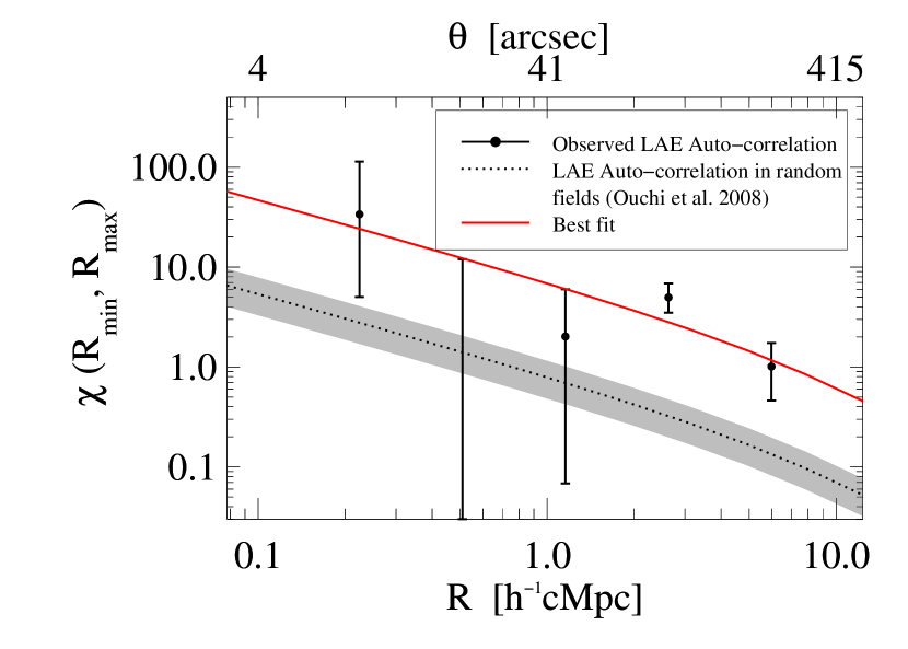
Figure 11.— LAE auto-correlation function in quasar fields. The filled circles are showing our measurement with $1\sigma$ Poisson error bars and the red curve shows the best fit for our measurement given by $r^{GG}_{0}=9.12^{+1.32}_{-1.31}\,h^{-1}$ cMpc for a fixed slope at $\gamma=1.8$. The dotted black line shows the observed LAE auto−correlation in blank fields at $z\sim 4$ measured by Ouchi et al. (2010) with the gray shaded area indicating the 1$\sigma$ errors based on their $1\sigma$ error reported for $r^{GG}_{0}$. We find that LAEs are significantly more clustered in quasar fields compared with their clustering in blank fields.

Table 6LAEs Auto-Correlation Function.

$R_{\rm min}$	$R_{\rm max}$	$\langle GG\rangle$	$\langle RR\rangle$	$\chi(R_{\rm min},R_{\rm max})$
$(h^{-1}$ cMpc)	$(h^{-1}$ cMpc)
0.136	0.308	1	0.029	33.760${}^{+79.947}_{-28.746}$
0.308	0.700	0	0.142	-1.000${}^{+12.980}_{-0.000}$
0.700	1.591	2	0.663	2.018${}^{+3.981}_{-1.950}$
1.591	3.614	16	2.680	4.970${}^{+1.895}_{-1.477}$
3.614	8.211	13	6.460	1.012${}^{+0.728}_{-0.551}$

Note. — LAE auto-correlation function in quasars fields $\chi(R_{\rm min},R_{\rm max})$ shown in Fig. 11.

Analogous to what we performed for the cross-correlation, we used a maximum likelihood estimator for a Poisson distribution to fit our auto-correlation function. We fix the slope at $\gamma=1.8$ and find a correlation length of $r^{GG}_{0}=9.12^{+1.32}_{-1.31}\,h^{-1}$ cMpc plotted as a red line in Fig. 11.

The measured value for the volume-averaged auto-correlation function at $z\sim 4$ is compared to our measurements in Fig. 11. Here we plugged in the best-fit LAE auto-correlation function parameters measured at $z\sim 4$ by Ouchi et al. (2010) ($r^{GG}_{0}=2.74^{+0.58}_{-0.72}\,h^{-1}\,{\rm cMpc}$ and $\gamma=1.8$) into eqn. (3) using a power law form for $\xi_{GG}(R,Z)$, which gives the dotted line plotted in Fig. 11. We find that LAEs are significantly more clustered in quasar fields compared with their clustering measured in blank fields. The fact that our measurements lie well above the Ouchi et al. (2010) values is again a manifestation of the overdensities of LAEs that we have uncovered around quasars.

IV.3. Systematic Errors in our Measurements

Our clustering analysis indicate that on the scales that we have probed ($R\lesssim 7\,h^{-1}\,{\rm cMpc}$) we detect an enhancement of LAEs centered on quasars revealed by their spatial profile consistent with a power-law shape in the cross-correlation measurement (see Fig. 10). However, the naive expectation of a deterministic bias model, whereby LAEs and quasars probe the same underlying dark mater overdensities, overpredicts the clustering of LAEs around quasars, with a correlation length $2.8$ times higher than the one measured in this work. Before discussing the implications of this discovery in section  § V, it is important to establish that it is not a result of systematic errors in our analysis. There are several possible systematics which could impact our results, which we discuss in turn.

First and foremost, are systematics associated with comparing LAEs selected from one survey to the background number density determined from another distinct survey. As discussed in section  § III.1, the preferred method would be to estimate the background directly from the same observations used to conduct the clustering analysis. This is possible provided either that the field-of-view of the images is large enough that one asymptotes to the background level in the outermost regions (i.e. where the clustering becomes vanishingly small), or if one has images with the same observational setup of blank fields. In both cases, the systematic errors associated with the background number density computation, coming from data reduction, source detection (for example SExtractor parameters that were used), photometry (e.g. aperture where colors are measured), LAE selection (i.e. color criteria, SExtractor flags, ${\rm S/N}$ ratio of the selected sources, etc.), and photometric completeness computation drop out of the problem, since one performs those steps in exactly the same manner for regions near quasars as for the background, i.e. the clustering measurement is essentially a relative measurement.

However, when the background level is computed from published luminosity functions determined from a distinct blank field analysis, these sources of systematics can creep in, because quasar fields could be analyzed differently than the background fields. Our study potentially suffers from this systematic, since the small field-of-view of FORS corresponding to $\sim 9.8\times 9.8\,h^{-2}{\rm cMpc}^{2}$ precludes a background measurement from our quasar fields, and we have no blank field pointings with our observational setup. In order to mitigate against this source of systematic error, we carefully tailored our LAE selection to mimic the selection adopted by Ouchi et al. (2008) on which our background computation is based, ensuring that we select LAEs with the same distribution of equivalent widths and hence abundance, as we detailed in § III.1 and § III.2.

Another systematic error that could lead us to underestimate the LAE clustering is one associated with the computation of the photometric completeness. If we were significantly overestimating the completeness in the source detection, then the completeness-corrected number density in blank fields computed from Ouchi et al. (2008) would be overestimated and it would result in a much lower clustering. Note also that if the sample were highly complete, the computation of number counts in the background would not be highly sensitive to uncertainties in the completeness, however, if the sample were highly incomplete, the number counts would be highly sensitive to it. Given that the median completeness at our 5$\sigma$ flux limit is only $<10$% (see Fig. 4), then when computing the blank field number density we are performing large corrections in the number counts predicted by the luminosity function measured by Ouchi et al. (2008) which could be affected by large uncertainties. To address this possibility, and check that our large completeness correction is not strongly affecting our background estimation, we also performed our clustering analysis using two brighter LAE samples where the completeness is $\sim 50$% (corresponding to a median limiting magnitude HeI$\sim 24.02$) and $\sim 80$% (corresponding to a median limiting magnitude HeI$\sim 23.84$) which are composed of a total of 21 and 15 LAEs, respectively. When computing $n_{\rm G}$, we then integrated the luminosity function up to such brighter magnitudes, and then compute the quasar-LAE cross-correlation for both cases, which are shown in Fig.  12. If the completeness computation were inaccurate, then for the 50% and 80% complete samples, for which we avoid to perform large corrections, we would expect to obtain different clustering than the one computed in § IV.1 (for which the sample is $\lesssim 10$% complete). For both cases, we get similar results and verified that the parameter constraints do not change significantly which suggests that the completeness computation (and therefore the completeness-corrected number density $n_{\rm G}$) is not uncertain and that this is not a significant source of systematic error in this work.

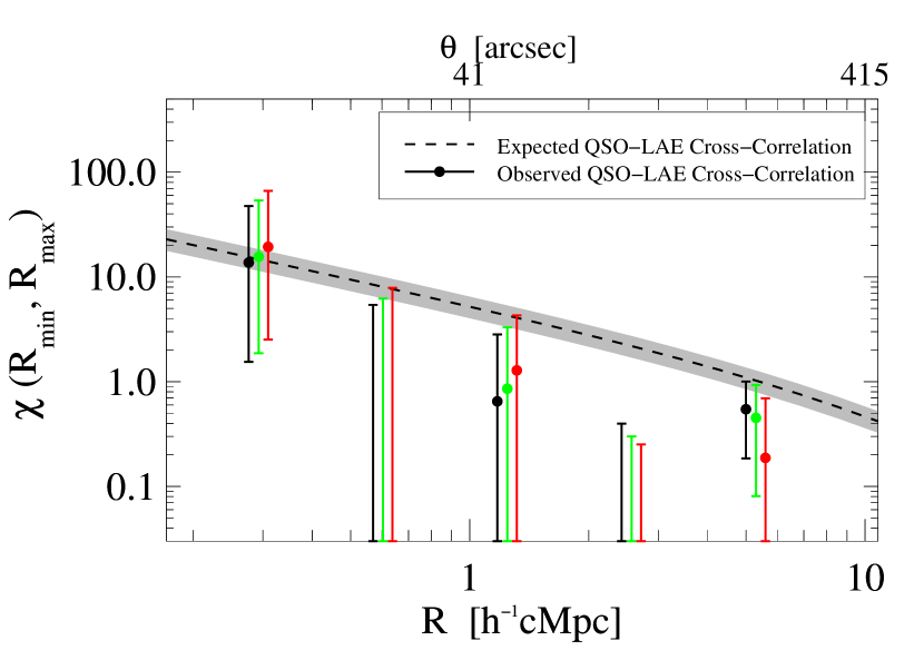
Figure 12.— Quasar-LAE cross-correlation function for three different LAEs samples. Black, green and red points show the cross-correlation function measured for a LAE sample $\lesssim 10\%$, $\sim 50\%$ and $\sim 80\%$ complete respectively. We slightly offset the points on the x-axis for clarity. The dashed black line shows the theoretical expectation of $\chi$ for our 17 stacked fields computed from the quasar and LAEs auto-correlation functions and assuming a deterministic bias model (see § IV.1). We obtain consistent clustering when we variate the limiting magnitude (and then the completeness correction) of the LAEs sample, which suggests that uncertainties in the completeness computation is not an important source of systematic errors in our measurement.

Finally, an important issue is the accuracy of the quasar redshifts. Large offsets between the quasar systemic redshift and the wavelengths covered by our NB filter would imply that we are actually selecting LAEs at sightly higher or lower redshifts, and hence at much larger radial distances where the clustering signal would be vanishingly small, such that the background number density of LAEs would be expected. As described in § II.1, we computed the quasar systemic redshift by using a custom line-centering code to determine the centroids of emission lines (instead of using only the peaks of them), and used the calibration of emission line shifts from Shen et al. (2007). Additionally, we have selected only quasars with low redshift errors, and only considered quasars for which the redshifted Ly$\alpha$ line of LAEs would land at the center of our NB filter (see Fig. 1). All of these precautions considerably reduce the possibility that redshift errors are biasing our analysis. Also note that for three out of 17 quasars the redshift has been measured only using the CIV emission line (considered to be the poorest redshift indicator), but for two of those fields (SDSSJ0119–0342 and SDSSJ0850+0629) we have detected an overdensity of LAEs greater than two, which indicates that we are actually selecting LAEs in the quasar environment. In general, we do not detect a correlation between the quasar redshift uncertainty (reported in Table  1) and the amplitude of the overdensity detected in their environment (reported in Table  4).

To summarize, we are confident that systematic errors associated with the background determination, completeness corrections, and imprecise quasar redshifts do not significantly impact our clustering measurements.

V. Discussion

The enhancement of LAEs in quasar fields (by a factor of 1.4 compared with the LAE number density in blank fields), the positive quasar-LAE cross-correlation function (with correlation length $r^{QG}_{0}=2.78^{+1.16}_{-1.05}\,h^{-1}\,{\rm cMpc}$ for a fixed slope of $\gamma=1.8$), and the strong LAE auto-correlation function (with an auto-correlation length 3.3 times higher than the LAE auto-correlation length measured in blank fields) detected in this work are all indicators that quasars trace massive dark matter halos in the early universe. However, our results are in disagreement with the expected quasar-LAE cross-correlation function computed assuming a deterministic bias model, which overpredicts the cross-correlation function by a factor of 6.4, as shown by the dashed line in Fig. 10. In this section, we discuss some possible explanations for this discrepancy.

The first possible explanation is that previous clustering measurements at $z\sim 4$ (and used in this work) could suffer from some systematic errors. If either the quasar clustering (from Shen et al., 2007), or the LAE clustering (from Ouchi et al., 2010)), or both, were overestimated, we would still expect an enhancement of LAEs in quasars fields over the background value, but the expected quasar-LAE cross-correlation function computed in section IV would be overestimated. Specifically, for a deterministic bias model, where the cross-correlation function can be written as $\xi_{QG}=\sqrt{\xi_{QQ}\xi_{GG}}$, a discrepancy of a factor of 6.4 between our measured cross-correlation function $\chi(R_{\rm min},R_{\rm max})$ and the expected one can be explained by an overestimation of the product $\xi_{QQ}\xi_{GG}$ by a factor of $6.4^{2}=40.96$, implying that either the quasar or LAE correlation function (or both) would have to have been highly overestimated. An overestimate of this magnitude in the clustering of quasars or LAEs seems very unlikely and is highly inconsistent with the 1$\sigma$ quoted errors of previous works (represented by the gray shaded region in Fig. 10, which is computed by error propagation based on the reported $1\sigma$ errors of the $r^{QQ}_{0}$ and $r^{GG}_{0}$ parameters). Additionally, studies of high-redshift binary quasars, which provides an independent constraint on the quasar auto-correlation agree with the strong clustering reported in Shen et al. (2007) (Hennawi et al., 2010; McGreer et al., 2016).

Excluding the possibility of large errors in previous auto-correlation measurements, it seems that the only explanation would be that the simple deterministic bias picture that we have assumed breaks down. This is in apparent contradiction of the recent work by (García-Vergara et al., 2017) who measure the cross-correlation of LBGs with quasars and found $r^{QG}_{0}=8.83^{+1.39}_{-1.51}\,h^{-1}\,{\rm Mpc}$ (for a fixed $\gamma=2.0$), which is actually in good agreement with the deterministic bias and the equation $\xi_{QG}=\sqrt{\xi_{QQ}\xi_{GG}}$.

Thus it seems that while LGBs are clustered around quasars in the right numbers, it appears that LAEs may be avoiding quasar environments, at least on scales of $\lesssim 7\,h^{-1}$ cMpc. Other searches for LAEs in high-redshift quasar fields at physical scales comparable to those probed by our study also show that LAEs could be avoiding quasar environments, since the reported LAE number densities agrees with the expectations from blank fields (Bañados et al., 2013; Mazzucchelli et al., 2017). However conversely, Swinbank et al. (2012) detect a significant LAE overdensity in a $z=4.5$ quasar field. If we consider studies performed at larger scales ($R\lesssim 25\,h^{-1}$ cMpc), there are only few targeted LAEs in high-redshift ($z>4$) quasar environments. Some work finds that on larger scales LAE overdensities are not present (Kikuta et al., 2017; Goto et al., 2017; Ota et al., 2018) or that LAEs are distributed around the quasar but avoid their vicinity within $R<4.5$ cMpc (Kashikawa et al., 2007). In summary, studies of the clustering of LAEs around high-redshift quasars paint a confusing picture. We note that all of the aforementioned work focused on just one or two quasar fields, and considering the large cosmic variance observed in our sample (see Table 4), it is perhaps not surprising that the results are not conclusive. More work is still required with much larger statistical samples.

It is possible that some extra piece of physics acting on the scales probed in our work could be responsible for reducing the clustering of LAEs around quasars, causing the deterministic bias picture to break down. There are some theoretical ideas about how quasar feedback might suppress star formation in the vicinity of a quasar (e.g Francis & Bland-Hawthorn, 2004; Bruns et al., 2012), or how star formation in galaxies located in dense fields could be affected via environmental quenching (e.g. Peng et al., 2010). In both cases, we would expect a reduced number of galaxies in our fields compared with the deterministic bias model predictions, but the aforementioned physical processes would need to be impacting neighboring galaxies at the relatively large scales probed by our study ($\lesssim 7\,h^{-1}$ cMpc). However, it is hard to understand why these processes would impact LAEs differently from LBGs, which appear to obey deterministic bias. Additionally, the quasar feedback scenario seems inconsistent with the power-law shape for the quasar-LAE cross-correlation detected in our work (see Fig. 10), whereby LAEs tend to be preferentially clustered (relative to the random expectation) very close to the quasar (see also Fig. 8).

One possible explanation for the detection of fewer LAEs in $z\sim 4$ quasars environments might relate to the fact that the escape of Ly$\alpha$ photons is particularly sensitive to the presence of dust. If galaxies in the Mpc-scale quasar environments are on average significantly more dusty, this could suppress the number of detected LAEs, and explain why LBGs are less impacted. Indeed, some studies of quasar environments at $z\gtrsim 4$ report the detection of close submillimeter galaxies (SMGs) companions on scales of $R\lesssim 0.5$ cMpc (e.g. Trakhtenbrot et al., 2017; Decarli et al., 2017; Bischetti et al., 2018), some of which are totally extincted or at least very faint in the rest-frame UV. The acquisition of data at radio/submillimeter wavelengths in our quasar fields would allow one to explore this possibility, and would allow measurement of the clustering properties of both optical and dusty galaxy populations around quasars simultaneously.

VI. Summary

We studied the environment of 17 quasars at $z\sim 4$ in order to make the first measurement of the quasar-LAE cross-correlation function. We imaged the quasar fields using a NB filter on VLT/FORS2, to select LAEs at $z=3.88$. We carefully chose the quasar targets to have the Ly$\alpha$ line located in the center of our NB filter and to have small ($\rm 800\,km\,s^{-1}$) redshift uncertainties in order to ensure that the selected LAEs are associated with the central quasar.

LAE selection was performed to match the criteria used by Ouchi et al. (2008) who selected LAEs at $z\sim 4$ using the filter system (V, NB570, B) to measure the LAE luminosity function. Performing an analogous selection ensures that we obtain an LAE sample with the same color completeness and contamination levels. This allows us to simply use the Ouchi et al. (2008) luminosity function to compute the blank field LAE number counts and perform a robust clustering analysis. We select LAEs to have an (rest-frame) EW${}_{\rm Ly\alpha}>28$Å  and find 25 in our fields. Given our survey volume and completeness, the number of LAEs expected in blank fields is 18.36. Thus on average our work shows the quasar environment is overdense by a factor of 1.4, indicating that quasars inhabit massive dark matter halos in the young universe. Considering our fields individually, we find that 10 out of 17 fields are underdense, whereas the rest are overdense, demonstrating that cosmic variance is large, and a significant source of noise in studies of quasar environs. Studies at $z\sim 6$ often come to conclusions about quasar environments based on studying a single or handfuls of quasar fields, but the large cosmic variance we observe cautions one against over-interpreting such small samples.

We measured the quasar-LAE cross-correlation function and find it is consistent with a power-law shape, with correlation length of $r^{QG}_{0}=2.78^{+1.16}_{-1.05}\,h^{-1}\,{\rm cMpc}$ for a fixed slope of $\gamma=1.8$. For comparison, we also computed the expected quasar-LAE cross-correlation function assuming a deterministic bias model, and we find that this overpredicts the cross-correlation function by a factor of 6.4 in comparison with what is measured in this work, or equivalently, a factor of 2.1 in the overall number of galaxies. We also measure the LAE auto-correlation in quasar fields and find a correlation length of $r^{GG}_{0}=9.12^{+1.32}_{-1.31}\,h^{-1}$ cMpc which is $3.3$ times higher than the LAE correlation length measured in blank fields, providing further confirmation that quasars are indeed tracing biased regions of the universe.

We discussed possible reasons why the deterministic bias picture could break down for LAEs, although it is puzzling that it appears to hold for LBGs. If feedback or something specific to the quasar environment is responsible for preferentially suppressing LAE clustering around quasars, then this effect ought to only act within some “sphere of influence” around the quasar. Hence a larger scale study of the clustering of both LAE and LBGs that extends beyond the scales probed here ($R\lesssim 7\,h^{-1}\,{\rm cMpc}$) would be particularly illuminating. It may also be that LAEs are absent in the quasar environment because galaxies near quasars are on average more dusty. Future radio and submillimeter studies of these quasar fields would allow one to measure the clustering of both radio/submillimeter and optical selected galaxy populations simultaneously, which is an important avenue for future work.

References

- Adams et al. (2015) Adams, S. M., Martini, P., Croxall, K. V., Overzier, R. A., & Silverman, J. D. 2015, MNRAS, 448, 1335
- Adelberger & Steidel (2005) Adelberger, K. L., & Steidel, C. C. 2005, ApJ, 630, 50
- Angulo et al. (2012) Angulo, R. E., Springel, V., White, S. D. M., et al. 2012, MNRAS, 425, 2722
- Appenzeller & Rupprecht (1992) Appenzeller, I., & Rupprecht, G. 1992, The Messenger, 67, 18
- Bañados et al. (2013) Bañados, E., Venemans, B., Walter, F., et al. 2013, ApJ, 773, 178
- Balmaverde et al. (2017) Balmaverde, B., Gilli, R., Mignoli, M., et al. 2017, A&A, 606, A23
- Becker et al. (1995) Becker, R. H., White, R. L., & Helfand, D. J. 1995, ApJ, 450, 559
- Bertin (2006) Bertin, E. 2006, in Astronomical Society of the Pacific Conference Series, Vol. 351, Astronomical Data Analysis Software and Systems XV, ed. C. Gabriel, C. Arviset, D. Ponz, & S. Enrique, 112
- Bertin & Arnouts (1996) Bertin, E., & Arnouts, S. 1996, A&AS, 117, 393
- Bertin et al. (2002) Bertin, E., Mellier, Y., Radovich, M., et al. 2002, in Astronomical Society of the Pacific Conference Series, Vol. 281, Astronomical Data Analysis Software and Systems XI, ed. D. A. Bohlender, D. Durand, & T. H. Handley, 228
- Bischetti et al. (2018) Bischetti, M., Piconcelli, E., Feruglio, C., et al. 2018, A&A, 617, A82
- Bouwens et al. (2007) Bouwens, R. J., Illingworth, G. D., Franx, M., & Ford, H. 2007, ApJ, 670, 928
- Bouwens et al. (2009) Bouwens, R. J., Illingworth, G. D., Franx, M., et al. 2009, ApJ, 705, 936
- Bouwens et al. (2010) Bouwens, R. J., Illingworth, G. D., Oesch, P. A., et al. 2010, ApJ, 709, L133
- Brammer et al. (2008) Brammer, G. B., van Dokkum, P. G., & Coppi, P. 2008, ApJ, 686, 1503
- Bruns et al. (2012) Bruns, L. R., Wyithe, J. S. B., Bland-Hawthorn, J., & Dijkstra, M. 2012, MNRAS, 421, 2543
- Bruzual & Charlot (2003) Bruzual, G., & Charlot, S. 2003, MNRAS, 344, 1000
- Capak et al. (2011) Capak, P. L., Riechers, D., Scoville, N. Z., et al. 2011, Nature, 470, 233
- Cardelli et al. (1989) Cardelli, J. A., Clayton, G. C., & Mathis, J. S. 1989, ApJ, 345, 245
- Cassata et al. (2011) Cassata, P., Le Fèvre, O., Garilli, B., et al. 2011, A&A, 525, A143
- Chabrier (2003) Chabrier, G. 2003, PASP, 115, 763
- Chiang et al. (2013) Chiang, Y.-K., Overzier, R., & Gebhardt, K. 2013, ApJ, 779, 127
- Coatman et al. (2017) Coatman, L., Hewett, P. C., Banerji, M., et al. 2017, MNRAS, 465, 2120
- Coil et al. (2007) Coil, A. L., Hennawi, J. F., Newman, J. A., Cooper, M. C., & Davis, M. 2007, ApJ, 654, 115
- Dawson et al. (2013) Dawson, K. S., Schlegel, D. J., Ahn, C. P., et al. 2013, AJ, 145, 10
- Decarli et al. (2017) Decarli, R., Walter, F., Venemans, B. P., et al. 2017, Nature, 545, 457
- Drake et al. (2017) Drake, A. B., Garel, T., Wisotzki, L., et al. 2017, A&A, 608, A6
- Eftekharzadeh et al. (2015) Eftekharzadeh, S., Myers, A. D., White, M., et al. 2015, MNRAS, 453, 2779
- Eisenstein et al. (2011) Eisenstein, D. J., Weinberg, D. H., Agol, E., et al. 2011, AJ, 142, 72
- Ferrarese & Merritt (2000) Ferrarese, L., & Merritt, D. 2000, ApJ, 539, L9
- Francis & Bland-Hawthorn (2004) Francis, P. J., & Bland-Hawthorn, J. 2004, MNRAS, 353, 301
- Fukugita et al. (1995) Fukugita, M., Shimasaku, K., & Ichikawa, T. 1995, PASP, 107, 945
- García-Vergara et al. (2017) García-Vergara, C., Hennawi, J. F., Barrientos, L. F., & Rix, H.-W. 2017, ApJ, 848, 7
- Gaskell (1982) Gaskell, C. M. 1982, ApJ, 263, 79
- Gebhardt et al. (2000) Gebhardt, K., Bender, R., Bower, G., et al. 2000, ApJ, 539, L13
- Gehrels (1986) Gehrels, N. 1986, ApJ, 303, 336
- Goto et al. (2017) Goto, T., Utsumi, Y., Kikuta, S., et al. 2017, MNRAS, 470, L117
- Hamuy et al. (1994) Hamuy, M., Suntzeff, N. B., Heathcote, S. R., et al. 1994, PASP, 106, 566
- Hamuy et al. (1992) Hamuy, M., Walker, A. R., Suntzeff, N. B., et al. 1992, PASP, 104, 533
- He et al. (2018) He, W., Akiyama, M., Bosch, J., et al. 2018, PASJ, 70, S33
- Hennawi et al. (2006) Hennawi, J. F., Prochaska, J. X., Burles, S., et al. 2006, ApJ, 651, 61
- Hennawi et al. (2010) Hennawi, J. F., Myers, A. D., Shen, Y., et al. 2010, ApJ, 719, 1672
- Husband et al. (2013) Husband, K., Bremer, M. N., Stanway, E. R., et al. 2013, MNRAS, 432, 2869
- Ikeda et al. (2015) Ikeda, H., Nagao, T., Taniguchi, Y., et al. 2015, ApJ, 809, 138
- Kashikawa et al. (2007) Kashikawa, N., Kitayama, T., Doi, M., et al. 2007, ApJ, 663, 765
- Kashikawa et al. (2006) Kashikawa, N., Yoshida, M., Shimasaku, K., et al. 2006, ApJ, 637, 631
- Kikuta et al. (2017) Kikuta, S., Imanishi, M., Matsuoka, Y., et al. 2017, ApJ, 841, 128
- Kim et al. (2009) Kim, S., Stiavelli, M., Trenti, M., et al. 2009, ApJ, 695, 809
- Madau (1995) Madau, P. 1995, ApJ, 441, 18
- Magorrian et al. (1998) Magorrian, J., Tremaine, S., Richstone, D., et al. 1998, AJ, 115, 2285
- Mazzucchelli et al. (2017) Mazzucchelli, C., Bañados, E., Decarli, R., et al. 2017, ApJ, 834, 83
- McGreer et al. (2016) McGreer, I. D., Eftekharzadeh, S., Myers, A. D., & Fan, X. 2016, AJ, 151, 61
- Metcalfe et al. (2001) Metcalfe, N., Shanks, T., Campos, A., McCracken, H. J., & Fong, R. 2001, MNRAS, 323, 795
- Mo & White (1996) Mo, H. J., & White, S. D. M. 1996, MNRAS, 282, 347
- Morselli et al. (2014) Morselli, L., Mignoli, M., Gilli, R., et al. 2014, A&A, 568, A1
- Myers et al. (2006) Myers, A. D., Brunner, R. J., Richards, G. T., et al. 2006, ApJ, 638, 622
- Oke (1974) Oke, J. B. 1974, ApJS, 27, 21
- Oke (1990) —. 1990, AJ, 99, 1621
- Ota et al. (2018) Ota, K., Venemans, B. P., Taniguchi, Y., et al. 2018, ApJ, 856, 109
- Ouchi et al. (2004a) Ouchi, M., Shimasaku, K., Okamura, S., et al. 2004a, ApJ, 611, 660
- Ouchi et al. (2004b) —. 2004b, ApJ, 611, 685
- Ouchi et al. (2008) Ouchi, M., Shimasaku, K., Akiyama, M., et al. 2008, ApJS, 176, 301
- Ouchi et al. (2010) Ouchi, M., Shimasaku, K., Furusawa, H., et al. 2010, ApJ, 723, 869
- Ouchi et al. (2018) Ouchi, M., Harikane, Y., Shibuya, T., et al. 2018, PASJ, 70, S13
- Overzier et al. (2008) Overzier, R. A., Bouwens, R. J., Cross, N. J. G., et al. 2008, ApJ, 673, 143
- Padmanabhan et al. (2009) Padmanabhan, N., White, M., Norberg, P., & Porciani, C. 2009, MNRAS, 397, 1862
- Pâris et al. (2014) Pâris, I., Petitjean, P., Aubourg, É., et al. 2014, A&A, 563, A54
- Patat et al. (2011) Patat, F., Moehler, S., O’Brien, K., et al. 2011, A&A, 527, A91
- Peng et al. (2010) Peng, Y.-j., Lilly, S. J., Kovač, K., et al. 2010, ApJ, 721, 193
- Planck Collaboration et al. (2018) Planck Collaboration, Aghanim, N., Akrami, Y., et al. 2018, arXiv e-prints, arXiv:1807.06209
- Porciani & Norberg (2006) Porciani, C., & Norberg, P. 2006, MNRAS, 371, 1824
- Richards et al. (2002) Richards, G. T., Fan, X., Newberg, H. J., et al. 2002, AJ, 123, 2945
- Schlegel et al. (1998) Schlegel, D. J., Finkbeiner, D. P., & Davis, M. 1998, ApJ, 500, 525
- Shanks et al. (2015) Shanks, T., Metcalfe, N., Chehade, B., et al. 2015, MNRAS, 451, 4238
- Shen et al. (2007) Shen, Y., Strauss, M. A., Oguri, M., et al. 2007, AJ, 133, 2222
- Shen et al. (2009) Shen, Y., Strauss, M. A., Ross, N. P., et al. 2009, ApJ, 697, 1656
- Shen et al. (2013) Shen, Y., McBride, C. K., White, M., et al. 2013, ApJ, 778, 98
- Shen et al. (2016) Shen, Y., Brandt, W. N., Richards, G. T., et al. 2016, ApJ, 831, 7
- Shibuya et al. (2019) Shibuya, T., Ouchi, M., Harikane, Y., & Nakajima, K. 2019, ApJ, 871, 164
- Shimasaku et al. (2006) Shimasaku, K., Kashikawa, N., Doi, M., et al. 2006, PASJ, 58, 313
- Simpson et al. (2014) Simpson, C., Mortlock, D., Warren, S., et al. 2014, MNRAS, 442, 3454
- Sobral et al. (2018) Sobral, D., Santos, S., Matthee, J., et al. 2018, MNRAS, 476, 4725
- Springel et al. (2005) Springel, V., Di Matteo, T., & Hernquist, L. 2005, MNRAS, 361, 776
- Stetson (2000) Stetson, P. B. 2000, PASP, 112, 925
- Stiavelli et al. (2005) Stiavelli, M., Djorgovski, S. G., Pavlovsky, C., et al. 2005, ApJ, 622, L1
- Swinbank et al. (2012) Swinbank, J., Baker, J., Barr, J., Hook, I., & Bland-Hawthorn, J. 2012, MNRAS, 422, 2980
- Trainor & Steidel (2012) Trainor, R. F., & Steidel, C. C. 2012, ApJ, 752, 39
- Trakhtenbrot et al. (2017) Trakhtenbrot, B., Lira, P., Netzer, H., et al. 2017, ApJ, 836, 8
- Tytler & Fan (1992) Tytler, D., & Fan, X.-M. 1992, ApJS, 79, 1
- Uchiyama et al. (2018) Uchiyama, H., Toshikawa, J., Kashikawa, N., et al. 2018, PASJ, 70, S32
- Utsumi et al. (2010) Utsumi, Y., Goto, T., Kashikawa, N., et al. 2010, ApJ, 721, 1680
- Vanden Berk et al. (2001) Vanden Berk, D. E., Richards, G. T., Bauer, A., et al. 2001, AJ, 122, 549
- Venemans et al. (2005) Venemans, B. P., Röttgering, H. J. A., Miley, G. K., et al. 2005, A&A, 431, 793
- Venemans et al. (2007) —. 2007, A&A, 461, 823
- White et al. (2008) White, M., Martini, P., & Cohn, J. D. 2008, MNRAS, 390, 1179
- White et al. (2012) White, M., Myers, A. D., Ross, N. P., et al. 2012, MNRAS, 424, 933
- Willott et al. (2005) Willott, C. J., Percival, W. J., McLure, R. J., et al. 2005, ApJ, 626, 657
- Worseck & Prochaska (2011) Worseck, G., & Prochaska, J. X. 2011, ApJ, 728, 23
- York et al. (2000) York, D. G., Adelman, J., Anderson, Jr., J. E., et al. 2000, AJ, 120, 1579
- Zheng et al. (2006) Zheng, W., Overzier, R. A., Bouwens, R. J., et al. 2006, ApJ, 640, 574