Asymmetric balance in symmetry breaking

Abstract

Spontaneous symmetry breaking is central to our understanding of physics and explains many natural phenomena, from cosmic scales to subatomic particles. Its use for applications requires devices with a high level of symmetry, but engineered systems are always imperfect. Surprisingly, the impact of such imperfections has barely been studied, and restricted to a single asymmetry. Here, we experimentally study spontaneous symmetry breaking with two controllable asymmetries. We remarkably find that features typical of spontaneous symmetry breaking, while destroyed by one asymmetry, can be restored by introducing a second asymmetry. In essence, asymmetries are found to balance each other. Our study illustrates aspects of the universal unfolding of the pitchfork bifurcation, and provides new insights into a key fundamental process. It also has practical implications, showing that asymmetry can be exploited as an additional degree of freedom. In particular, it would enable sensors based on symmetry breaking or exceptional points to reach divergent sensitivity even in presence of imperfections. Our experimental implementation built around an optical fiber ring additionally constitutes the first observation of the polarization symmetry breaking of passive driven nonlinear resonators.

Introduction

Spontaneous symmetry breaking (SSB) is a concept of fundamental importance Anderson (1972); Strocchi (2008); Malomed (2013). It is central to the standard model of particle physics Nambu (2009); Englert and Brout (1964); *higgs_broken_1964; Bernstein (1974), underpins phenomena as diverse as ferromagnetism and superconductity Landau and Lifshitz (1980); Tilley and Tilley (1990); Leggett and Sols (1991), and plays a key role in convection cells and fluid mechanics Crawford and Knobloch (1991), morphogenesis Turing (1952), embryo development Korotkevich et al. (2017), and more generally self-organization Prigogine et al. (1969). SSB can also be exploited for many applications Kaplan and Meystre (1981); Liu et al. (2014); Hamel et al. (2015); Cao et al. (2017); Del Bino et al. (2017); Woodley et al. (2018). In particular, new unique ways to manipulate light have recently been demonstrated in structures engineered to exhibit parity-time ($\mathcal{PT}$) symmetry breaking Feng et al. (2014); *hodaei_parity-timesymmetric_2014. Engineered systems however often exhibit deviations from perfect symmetry because of naturally occurring imperfections Kondepudi et al. (1986); D’Angelo et al. (1992). Surprisingly, the impact of asymmetries on SSB-related dynamics has barely been considered in experiments, and essentially restricted to situations with only one asymmetry parameter D’Angelo et al. (1992); Gelens et al. (2010). One exception are results obtained by Benjamin four decades ago on Couette flow between rotating cylinders, which are clearly linked to the presence of two imperfections, albeit only one was controlled Benjamin (1978a); *benjamin_bifurcation_1978-1. Here, we report for the first time an experimental study of a system that exhibits spontaneous mirror-symmetry breaking with two fully controllable asymmetry parameters. While the characteristic dynamics of SSB — random, spontaneous selection between two mirror-like states with opposite symmetries — are destroyed by one asymmetry, we remarkably observe that a second asymmetry can restore them. In essence, the two asymmetries can balance each other. Interestingly, this is conceptually related to the design principle of asymmetric balance, by which a design or an art composition can be asymmetric, and yet, still look balanced Pipes (2003).

Spontaneous symmetry breaking is underlain by the fundamental pitchfork bifurcation Strogatz (1994). For a system with left/right or mirror symmetry, that bifurcation describes how a symmetric state transitions to two equivalent, stable, mirror-like asymmetric states [see, e.g., panel (b) of Fig. 1]. The pitchfork is however a structurally fragile, degenerate bifurcation: in the presence of small asymmetries, one of the asymmetric states dominates while the other cannot be spontaneously excited Hirsch et al. (1977); Benjamin (1978a); *benjamin_bifurcation_1978-1; Golubitsky and Schaeffer (1979); *golubitsky_singularities_1985. It turns out that only two parameters are needed to describe all the possible topologies of the perturbed pitchfork — its so-called universal unfolding Benjamin (1978a); *benjamin_bifurcation_1978-1; Golubitsky and Schaeffer (1979); *golubitsky_singularities_1985; Ball (2001); Alam (2004). This argument has been used to reduce the number of parameters in the search of simplified models of complex problems, such as limb coordination Park and Turvey (2008) — a feature found in movements of a huge range of animals — or the emergence of the ubiquitous homochirality of biological molecules Ball and Brindley (2016); *lebreton_molecular_2018. It has also guided recent engineering research in buckling-resistant structures and led to the discovery that optimal designs with imperfect symmetry only emerge when considering two asymmetry parameters Várkonyi and Domokos (2007). We note that evolution, which is inherently guided by optimization, has produced countless designs with near but not perfect symmetry, including the functional neural wiring of the brain Várkonyi et al. (2006). Clearly, considering two asymmetry parameters instead of one in the study of SSB can have dramatic and intriguing consequences. To the best of our knowledge, our work is the first to experimentally address how two asymmetries can balance each other.

Polarization symmetry breaking

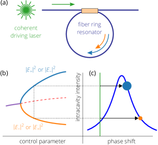
Figure 1: Illustration of polarization symmetry breaking. (a) Schematic diagram of a driven passive nonlinear fiber ring resonator. (b) Pitchfork bifurcation diagram showing how the intensities of the two polarization modes part above a certain threshold. The control parameter can be either the driving power or the driving laser frequency. (c) Resonance of the system illustrating how in an asymmetric state the stronger mode (large blue dot) can undergo a smaller effective nonlinear shift (black arrow) and be closer to resonance than the weaker mode (small orange dot). This occurs when the driving laser (green line) is red-detuned (left side of the resonance).

Our experiment is based on a passive nonlinear optical fiber ring resonator (akin to a Fabry-Pérot etalon) that presents two distinct orthogonal polarization modes. The resonator is externally, coherently driven by intense laser light [Fig. 1(a)] so as to excite both of these modes; hereafter $E_{+}$ and $E_{-}$ denote the modes’ complex electric field amplitudes inside the resonator. Ideally, when the two polarization modes are equally driven and are degenerate (i.e., the resonator material is isotropic, and the modes have identical resonance frequencies), the system is symmetric with respect to an interchange of the two modes, $E_{+}\rightleftarrows E_{-}$. In the simplest case, the stationary intracavity field solution assumes that symmetry, $E_{+}=E_{-}$, and the two modes have the same intensities. Symmetry breaking occurs above a certain threshold Areshev et al. (1983); Haelterman et al. (1994), and manifests itself by the parting of the intensities of the two polarization modes, $|E_{+}|^{2}\neq|E_{-}|^{2}$ [Fig. 1(b)]: the symmetric solution loses its stability in favor of two mirror-like asymmetric solutions. The instability stems from the cubic (Kerr) nonlinearity of silica optical fibers Agrawal (2013), by which the phase of one mode is affected by the intensity of the other (cross-phase modulation, or XPM). Critically, in optical fibers, XPM between polarization modes can be stronger than self-phase modulation (SPM) so that the weaker mode can experience a larger nonlinear phase shift than the stronger mode Agrawal (2013); Gilles et al. (2017). In these conditions, the weaker mode is pushed away from resonance while the stronger mode is pulled towards it, reinforcing any initial intensity imbalance [Fig. 1(c)] Del Bino et al. (2017). This polarization SSB is formally identical to the SSB that occurs in the same system when considering two counter-propagating beams Kaplan and Meystre (1982), and which was recently studied experimentally Del Bino et al. (2017). In both cases, an imbalance of driving power between the two modes (beams) readily provides a controllable asymmetry parameter. In our experiment, we have also manipulated the wavenumbers of the two driven polarization components as the second asymmetry parameter.

Passive driven scalar Kerr resonators can be efficiently described by a mean-field approach Lugiato and Lefever (1987); Haelterman et al. (1994). For two incoherently coupled polarization modes, assuming continuous-wave (cw) driving and neglecting chromatic dispersion, the evolution of $E_{+}$ and $E_{-}$ over time $t$ is given by (using the same normalization as in Leo et al. (2010)),

$$\frac{\partial E_{+}}{\partial t}=\left[-1+i(|E_{+}|^{2}+B|E_{-}|^{2}-\Delta_{+})\right]E_{+}+\sqrt{X}\cos\chi\,,$$ (1)

$$\frac{\partial E_{-}}{\partial t}=\left[-1+i(|E_{-}|^{2}+B|E_{+}|^{2}-\Delta_{-})\right]E_{-}+\sqrt{X}\sin\chi\,.$$ (2)

In these equations, the incoherent coupling between the two modes is determined by the XPM coefficient $B$ ($B$ > 1). Other terms on the right-hand side represent, respectively, losses, SPM, the detuning of the driving frequency with respect to resonance, and the driving strengths of each mode. Here $X$ represents the total driving power, while a driving power imbalance between the modes is accounted for by introducing an effective driving polarization ellipticity angle $\chi$. An ellipticity angle $\chi$ of $45^{\circ}$ represents perfectly balanced driving. Because of residual birefringence in our fiber resonator, the resonances of the two polarization mode families are normally observed for different driving laser frequencies, which correspond to having different detunings in the equations above, $\Delta_{+}\neq\Delta_{-}$. The difference in detuning, $\delta\Delta=\Delta_{+}-\Delta_{-}$, equivalently represents the difference in wavenumbers with which the two polarization components propagate inside the resonator (see Appendix A) and is our second asymmetry parameter. It is tuned in our experiment by shifting the carrier frequency of the $E_{-}$ mode with a frequency shifter as explained below. Symmetry for the interchange of the two modes in Eqs. (1)–(2) is obtained with $\chi=45^{\circ}$ and $\delta\Delta=0$. Note also the absence of rotational phase invariance in these equations because of the external driving terms, which is a key feature of the passive driven resonator considered here, in contrast to, e.g., laser resonators.

Experimental setup

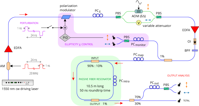
Figure 2: Experimental setup. PC: polarization controller, PBS: polarization beam-splitter, AM: amplitude modulator, AOM: acousto-optic modulator (frequency shifter), EDFA: Erbium-doped fiber amplifier, BPF: bandpass filter, OI: optical isolator. Blue lines: optical fibers, Green lines: polarization-maintaining (PM) optical fibers, Black lines: RF connections. The actual resonator is highlighted with a green background. Vertical (orange) and horizontal (blue) double-arrows symbolize the two different polarization modes at various places in the setup.

Figure 2 illustrates the experimental setup. The passive ring resonator (highlighted in green) has a total length of about $10.5$ m, corresponding to a free spectral range (FSR) of $19.76$ MHz ($\pm 20$ kHz) and a round trip time $t_{\mathrm{R}}$ of $50.60$ ns ($\pm 50$ ps). It is built around a fiber coupler (beam-splitter) that recirculates 90 % of the intracavity light, and allows for the injection of the coherent driving field (entering from the top right in the figure). Another 1 % tap coupler extracts a small fraction of the intracavity field for analysis through three photodiodes monitoring respectively the total output intensity as well as the individual intensities of the two polarization modes (more details are given below). The rest of the resonator is made up of “spun” single-mode silica optical fiber, a type of fiber which presents very little polarization anisotropy (birefringence) Barlow et al. (1981). At the 1550 nm driving wavelength, that fiber exhibits normal group-velocity dispersion ($-40\ \mathrm{ps/nm/km}$), which has been selected to avoid modulation instabilities Agrawal (2013). The measured resonator finesse is $24.1$ ($\pm 0.1$), amounting to total losses of 26 % per roundtrip. The associated photon lifetime and resonance linewidth are, respectively, about $4\,t_{\mathrm{R}}$ and 820 kHz. The resonance linewidth is much broader than that of our driving laser, a distributed-feedback cw Erbium-doped fiber laser (Koheras AdjustiK E15), with a linewidth ${<1}$ kHz, therefore guaranteeing coherent driving. The driving laser frequency can be tuned via a piezo-electric actuator, which offers a simple way to scan the cavity resonances.

Due to unavoidable fiber bending and other imperfections, the two polarization modes of the resonator are slightly linearly coupled Pierce (1954). As a consequence, the interactions between the two modes are not only dependent on the modal intensities as described above, but are also phase sensitive Cao et al. (2017). To avoid this complication, we drive the two polarization modes with slightly different carrier frequencies. At the same time, we purposefully introduce some fixed birefringence in the resonator through an intracavity polarization controller Lefevre (1980), $\mathrm{PC_{intra}}$ in Fig. 2, to counterbalance the associated difference in wavenumbers, and to realize effective isotropic (or close to isotropic) conditions for the two driven polarization components. In practice, we have separated the two families of orthogonally polarized cavity resonances by about 45 % of the FSR; the precise value is not critical. The dual carrier driving field is prepared, ahead of injection into the resonator, by splitting the output of the single frequency driving laser into two components with a polarization beam-splitter (PBS), and frequency-shifting one of these with an acousto-optic modulator (AOM). The other path incorporates a variable attenuator (V) set to introduce the same losses as the AOM. The two components are then recombined in a second PBS. Together with the use of polarization-maintaining fibers (shown in green in Fig. 2) in between the two PBSs, no polarization-dependent losses are introduced. Behind the second PBS, the two carriers have orthogonal polarization and are mapped onto the two resonator modes using another PC (labeled $\mathrm{PC_{map}}$ in Fig. 2), so that each drive a separate mode. $\mathrm{PC_{map}}$ is adjusted with the AOM off, which suppresses one of the polarization components of the driving beam, so as to excite a single family of cavity resonances, carefully canceling any trace of the other (orthogonally polarized) family through observation of the total output intensity.

Our experimental arrangement enables simple and reproducible control of the two asymmetry parameters. On the one hand, adjusting the RF frequency applied onto the AOM (around 80 MHz) controls the effective isotropy, specifically the difference in wavenumbers $\delta\Delta$ with which the two polarization components propagate inside the resonator. On the other hand, controlling the polarization state of the beam ahead of the first PBS changes the ratio of driving power between the two modes, or equivalently the driving ellipticity $\chi$, without affecting the total driving power. This is achieved with an electronic polarization modulator, complemented with a manual bias ($\mathrm{PC}_{\chi}$).

To calibrate the measurement of $\delta\Delta$, we first observe the AOM frequency at which the linear resonances of the two polarization modes overlap and have maximal total peak intensity; this point corresponds to $\delta\Delta=0$. Note that this calibration stage is performed when the resonator is operated purely in the linear regime. From that starting position, any change $\Delta f$ in the frequency applied to the AOM corresponds to a change of $\delta\Delta$ of $2\mathcal{F}(\Delta f/\mathrm{FSR})$ (see Appendix A). With the uncertainties quoted above for $\mathcal{F}$ and $\mathrm{FSR}$, this is obtained to within $0.5$ %.

Because of environmental fluctuations, the driving ellipticity $\chi$ typically slowly varies over time at the input of the resonator. To stabilize the system against these perturbations, we measure and monitor $\chi$ close to the resonator input, and apply appropriate feedback to the polarization modulator through a PID controller. The value of $\chi$ is obtained by tapping 1 % of the driving beam, and by measuring the intensities of the two polarization components of the light, separated with another PBS, with two carefully calibrated photodetectors. A PC ($\mathrm{PC_{monitor}}$ in Fig. 2) placed ahead of the PBS is adjusted such that each diode is only sensitive to one particular cavity polarization mode. Specifically, this is obtained by verifying that one of the photodiode reads zero when the AOM is off (a similar procedure was used to separate the modes at the output). We have made sure that the photodetectors are operated strictly in a linear regime. Also, we have measured a calibration factor that corrects for the small difference in responsitivities between the two diodes, so that we get the same reading when they are illuminated by the same intensity. Finally, before each set of measurements, we carefully measure the zero level of both diodes. $\tan^{2}\chi$ is then obtained as the ratio of the two photodiodes readings after zeroing and responsitivity correction. This leads to the value of $\chi$ with an uncertainty that we estimate at less than $0.5^{\circ}$. The experimental setup incorporates a second feedback loop (not shown in Fig. 2) that offers the possibility to lock the driving laser at a set detuning from resonance, using the method of Ref. Nielsen et al. (2018). Note that changing the laser frequency changes the two detunings $\Delta_{+}$ and $\Delta_{-}$, or equivalently the wavenumbers of the two driven polarization components, by the same amount and does not introduce any asymmetry. When both feedback loops are engaged, all the parameters of the resonator are quantifiably controlled and stable.

Finally, to reach more easily the peak power level necessary to observe SSB, the resonator is synchronously driven by flat-top $1.04$ ns long pulses carved into the cw beam of our driving laser with an amplitude modulator (AM). For reasons explained below, two such pulses are launched per roundtrip, separated by $24.5$ ns. The separation is chosen large enough to minimize unwanted ripples in the AM driving electronics, while at the same time avoiding the acoustic echo generated down the optical fibers by the leading pulse and that would affect the shape of the trailing pulse for separations in the 20–22 ns range Jang et al. (2013). The use of pulses also avoids the detrimental effect of stimulated Brillouin scattering that is typical of silica optical fibers, and which would otherwise deplete the driving beam Agrawal (2013). Calibration of the normalized driving power $X$ was obtained by observing the nonlinear shift of the resonance as a function of driving power. As our results do not fundamentally depend on $X$ (as long as it is set above the SSB threshold), for simplicity it was kept at the same level for all the measurements presented below. Specifically, we used $X=10.8$, which corresponds to about $2.7$ W of peak power (equivalent to 110 mW of total averaged power) at the resonator input. The nonlinear cross-coupling coefficient $B$ was obtained from the ratio of the nonlinear shift of the cavity resonance peak for balanced driving conditions ($\chi=45^{\circ}$) to that observed when only one mode was driven ($\chi=0^{\circ}$). That ratio is $(1+B)/2$, and is independent of driving power. Two separate measurements gave values of $B$ of $1.55$ and $1.6$, and the value was refined to $B=1.57$ ($\pm 0.01$) by fitting experimental data to the numerical model. Note that the occurrence of asymmetric balance does not depend critically on the actual value of $B$.

Results

We start by characterizing our system in symmetric conditions: the driving ellipticity $\chi$ is maintained at $45^{\circ}$ by the feedback loop while $\delta\Delta$ is set to zero. To this end, we repeatedly scan the driving laser frequency across several cavity resonances while resolving the two polarization modes (Fig. 3, blue and orange curves respectively). Here, the modal intensities are measured with slow photodiodes that do not resolve the individual driving pulses. Note that similar results would be obtained by scanning the driving power Haelterman et al. (1994). In Figs. 3(a) and 3(b), we present histograms of each mode intensity obtained by combining seven measurements comprising about 100 resonance scans each. Remarkably, while the two modes have equal intensities near the base of the resonance (in line with the symmetric conditions), the peak of the resonance exhibits a high degree of variability Juel et al. (1997). We observe that high intensity in one mode always correlates with low intensity in the other mode, as is made evident by the two individual scans shown in Figs. 3(c),(d): symmetry is markedly broken. Note that the scanning rate of 1 FSR per millisecond, corresponding to one resonance linewidth per 200 photon lifetime, is slow enough to guarantee that transients do not affect the mode selection.

In Figs. 3(c),(d), we have also plotted the total output intensity (black curves) measured at the resonator output. The total intensity does not display any sign of the underlying pitchfork instability, thus highlighting that the SSB studied here is a purely polarization phenomenon. To the best of our knowledge, this is the first observation of a polarization SSB in passive driven resonators, which was theoretically predicted more than three decades ago Areshev et al. (1983); Haelterman et al. (1994). Additionally, a comparison between Figs. 3(c) and 3(d) highlights the very high degree of mirror symmetry in our system, with the two sets of curves very nearly matching each other. The high variability in Figs. 3(a,b) can be interpreted as due to different subparts of the two pulses circling the resonator spontaneously breaking their symmetry one way or the other, randomly. Since these are not resolved by our slow photodetectors, this leads to averaged intensities spanning the entire range of values between those observed when pulses switch as a whole [panels (c) and (d) correspond to that latter case] even though the system has only two stationary solutions that are mirror of each other Haelterman et al. (1994). This latter fact will be formally confirmed below.

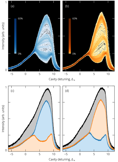
Figure 3: Nonlinear resonances in the spontaneous symmetry breaking regime illustrated by plotting averaged modal intensities (blue and orange curves) recorded as the cavity detuning is ramped up in symmetric conditions ($\chi=45^{\circ}$, $\delta\Delta=0$). In (a) and (b), measurements are taken over several hundreds of scans, and the data are presented as color-coded %-age-of-occurrence histograms. (c),(d) Two individual scans highlighting the anti-correlated behavior of the modal intensities, selected to illustrate the mirror symmetry of the system. The total intensity is also shown as black curves. Note: the orange curves are associated with the component up-shifted by the AOM.

Departing from symmetric conditions through a change in $\chi$ or $\delta\Delta$ leads to the disappearance of the behavior reported in Fig. 3. The system then always favors the same mode: resonance scans look either like the one presented in Fig. 3(c), or the one in Fig. 3(d), depending on the direction of the change Benjamin (1978a); Golubitsky and Schaeffer (1979); *golubitsky_singularities_1985. A secondary state, an almost mirror image of the first one, is never excited spontaneously although it might be present in the system Ball (2001); Gelens et al. (2010). In order to probe its existence under asymmetric conditions, and to identify all the cw stationary solutions of the system for each set of asymmetry parameters ($\chi$ and $\delta\Delta$), we proceeded as follows. With the detuning locked and total driving power kept constant, we measured the instantaneous output intensities of the two polarization components with 10 GHz-bandwidth photodiodes that resolve individual pulses, and acquired the data over about 8000 successive cavity round-trips with a 40 Gsample/s oscilloscope. In the middle of these acquisitions, we apply strong perturbations to the two driving pulses through the polarization modulator (see top left of Fig. 2) for about 100 roundtrips. The two pulses driving the resonator are subject to opposite perturbations to maximize the chance that one of the pulses will switch to the other solution, irrespective of which solution is initially spontaneously excited. For each oscilloscope trace, the instantaneous intensity levels of all the recorded pulses are then built into histograms, separately for the two pulses driving the resonator, and before and after the perturbation. Care is taken to avoid any transients following the perturbation, and pulses that are only partly switched. The maxima of the histograms allow us to identify the intensity levels of the steady-state stable asymmetric solutions for each polarization. Note that the use of two driving pulses provides two independent realizations of the experiment in the same conditions and clearly reveals the coexistence of the identified states. These measurements are repeated as we step $\chi$ (by adjusting the corresponding feedback loop setting point) and for different values of $\delta\Delta$.

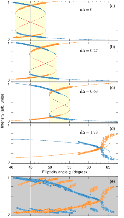
Figure 4: Measured modal intensities of identified stationary SSB solutions versus driving ellipticity $\chi$ for different values of $\delta\Delta$ and fixed frequency detuning $\Delta_{+}=5.45$. (a)–(d) Each solution is associated with two points (one for each mode, blue and orange) while different solutions are distinguished by using respectively darker round (when the “blue” mode dominates) and lighter square (“orange” dominates) symbols. Smooth lines correspond to theoretical predictions, with dashed lines denoting unstable states. The yellow band highlights the region of co-existence of states with opposite symmetries. (e) Combination of all the experimental results shown in (a)–(d), plus extra data obtained for $\delta\Delta=1.00$ and $1.49$.

The results are summarized in Fig. 4, where we plot the modal intensities of the identified stationary solutions (rounds and squares). The error level is indicated by the size of the markers. Panel 4(a) has been obtained with $\delta\Delta\simeq 0$. The two solutions identified for $\chi=45^{\circ}$ are exact mirror images of each other, as expected from perfect symmetry conditions (see Fig. 3). These measurements also confirm that in these conditions the system presents two and only two stable asymmetric solutions, validating our interpretation of the histograms above. As $\chi$ is varied around that point, we can observe that both solutions continue to exist, even though their degeneracy is lifted. Theoretical predictions (smooth curves) obtained by looking for the stationary solutions of Eqs. (1)–(2) for the experimental parameters agree very well with the measurements ($X=10.8$, $\Delta_{+}=5.45$, and $B$ fitted to $1.57$). Note that some solutions predicted theoretically are not observed in the experiment because they are only metastable in our pulsed driving conditions Garbin et al. (2017). The range of coexistence is highlighted as a yellow band, and is reasonably wide, covering almost $10^{\circ}$ of ellipticity change. Outside that band, however, the driving asymmetry becomes too strong, and only one solution remains: the symmetry breaking instability effectively disappears. In Fig. 4(b), we have introduced some asymmetry between the wavenumbers. Interestingly, we observe that the coexistence region seems to simply shift to a different range of values of $\chi$. In particular, there exists a value of $\chi\neq 45^{\circ}$ where the two solutions again appear to be mirror images of each other (where the blue and orange curves intersect). The two asymmetries, in $\chi$ and $\delta\Delta$, are now balancing each other. The balance can be realized continuously, i.e., for every value of $\delta\Delta$ within a certain range (see Appendix B for a geometric interpretation). It is also very robust: in Fig. 4(c), $\delta\Delta$ is large enough for the coexistence region not to even overlap with the balanced driving condition at $\chi=45^{\circ}$. Eventually, when too much asymmetry is present [Fig. 4(d)], the coexistence region disappears: symmetry breaking is well and truly destroyed and cannot be restored through a balance of asymmetries. Figure 4(e) highlights how all the experimental data in Figs. 4(a)–(d) (plus some extra measurements) fit together. We must stress that the theoretical fits shown in Fig. 4 have all been obtained for the same parameters values and with the values of $\delta\Delta$ directly measured experimentally. This makes the overall agreement quite remarkable.

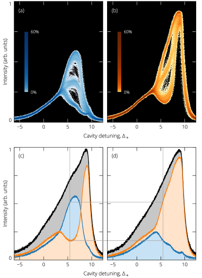
Figure 5: Same as Fig. 3 but under conditions of asymmetric balance, with $\delta\Delta=0.63$ [same value as in Fig. 4(c)] and $\chi=53.5^{\circ}$. These measurements illustrate that an SSB-like response can be found under asymmetric conditions when asymmetries in $\chi$ and $\delta\Delta$ are critically balanced. In particular, a “blue” dominated solution can still be spontaneously excited, (c), even though the “orange” mode is driven stronger. Grey lines in (c), (d) highlight how the two solutions observed for $\Delta=5.45$ are close mirror of each other, corresponding to the crossing point in Fig. 4(c).

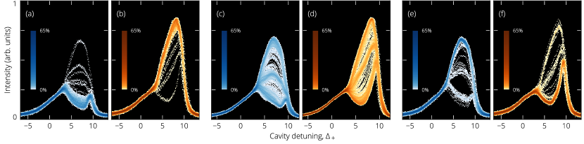
Figure 6: Resonance scan histograms of average modal intensity levels (same color scheme as other figures) observed when bracketing the asymmetric balance condition found with $\chi=48.5^{\circ}$ (1:$1.3$ driving power ratio). (a,b) $\delta\Delta=0.27-0.015$, and an “orange” dominated solution is favored. (c,d) $\delta\Delta=0.27$, asymmetric balance is realized. (e,f) $\delta\Delta=0.27+0.015$, and the solution is dominated by the “blue” mode. The histograms in balanced conditions include data from $650$ forward resonance scans each, while the other includes about 110 scans each. A change in $\delta\Delta$ of $0.015$ corresponds to a change of 6 kHz in the AOM driving frequency.

To explore further the regime of asymmetric balance, we performed additional resonance scan measurements with parameters close to those where we find mirror-like solutions. For $\delta\Delta=0.63$ [corresponding to Fig. 4(c)], this is illustrated in Fig. 5, using the same format as in Fig. 3. Remarkably, the histograms of Figs. 5(a,b) reveal that, for a critical value of driving ellipticity $\chi\simeq 53.5^{\circ}$, and despite the strong asymmetries, the system presents again a high degree of variability similar to that observed under symmetric conditions. The two individual scans plotted in Figs. 5(c) and 5(d) highlight that the observed variability stems from the random selection of one of two solutions of opposite symmetries, i.e., in which a different polarization mode dominates. The fact that the “orange” mode is driven more strongly than the “blue” mode (the driving ellipticity corresponds here to a factor of about $1.8$ difference in driving intensity) is evident in Fig. 5, yet it does not preclude a “blue” dominant solution to be spontaneously excited [Fig. 5(c)]. Similar to the symmetric case, and perhaps more remarkably, we again observe no sign of the instability in the total intensity [black curves in Figs. 5(c),(d)]. These results show that asymmetric balance means more than just restoring mirror-like solutions. A pitchfork-like spontaneous-selection dynamics is recovered when asymmetries are balanced. We note that this behavior agrees with what would be expected from the two-parameter unfolding of an imperfect pitchfork bifurcation Golubitsky and Schaeffer (1979); *golubitsky_singularities_1985. The bifurcation point in Figs. 5(a,b) where the mode selection takes place corresponds to what has been referred to as the “transcritical point” in Refs. Benjamin (1978a); *benjamin_bifurcation_1978-1. Note that the critical value of $\chi$ found in Fig. 5 ($53.5^{\circ}$) is slightly different with that observed to give mirror-like solutions in Fig. 4(c) ($51^{\circ}$), but this is consistent with the dependence of the critical point on the cavity detuning $\Delta_{+}$ and matches numerical predictions.

When slightly offset from asymmetric balance conditions, the system of course always favors one of the two solutions and, perhaps not unsurprisingly, a different mode is found to dominate for opposite directions of change. We illustrate this point in Fig. 6 for a different value of $\chi=48.5^{\circ}$, for which asymmetric balance is realized with $\delta\Delta=0.27$ [corresponding to Fig. 4(b)]. Figures 6(c,d) show histograms in balanced conditions for these parameters; the results are similar to those shown for $\delta\Delta=0.63$ in Fig. 5. In Figs. 6(a,b), $\delta\Delta=0.27-0.015$, and the system preferentially selects the solution for which the “orange” mode dominates, while the opposite occurs when $\delta\Delta=0.27+0.015$ [Figs. 6(e,f)]. The non-zero probability of occurrence of the other solution is due to noise in the system, and to the proximity to the critical point. We again note that all these findings align with what would be expected from a standard pitchfork, except that we are observing these behaviors in the presence of asymmetries.

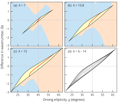
Figure 7: (a)–(c) Region of co-existence (yellow, surrounded by black line) of symmetry-broken mirror-like solutions in the $(\chi,\delta\Delta)$ parameter space evaluated numerically for different driving powers $X$, with $\Delta_{+}=5.45$ and $B=1.57$. The condition for asymmetric balance is shown as a red curve in each graph. Blue- and orange-shaded areas indicate which mode dominates outside the co-existence region. The white area indicates a region where there are no stable homogenous solutions. (d) Superposition of the limit of the co-existence regions, for driving power $X=6$–14, in step of 2 (outward).

At this point, it must be clear that our findings are not specific to the parameters of Figs. 5 or 6: spontaneous selection and a pitchfork-like dynamics can be restored over a continuous range of values of $\delta\Delta$ or driving power around those illustrated. In fact, no parameters need to take a specific value for the effects described here to be observed. This makes clear that our observations are not the result of an accidental symmetry. To illustrate this point further, we have calculated (using numerical continuation Doedel and Oldeman ) the limits of the regions of the $(\chi,\delta\Delta)$ asymmetry parameter space where Eqs. (1)–(2) exhibit co-existence of two stable mirror-like symmetry broken solutions, as well as the conditions in which asymmetric balance can be achieved. This is illustrated in Figs. 7(a)–(c), for different values of driving power $X$ and for a fixed detuning of the $+$ mode, $\Delta_{+}=5.45$, matching the experimental conditions. The black curves delineate the co-existence region, also highlighted with a yellow background; this region corresponds to that highlighted in a similar way in Fig. 4. In the co-existence region, we have also plotted as a red curve the combination of parameters for which asymmetric balance is achieved (strictly speaking, where the upper intensities of the two co-existing solutions match; see also Appendix B). Overall, these plots illustrate the wide range of parameters for which asymmetric balance can be realized. Just outside the co-existence region, only one stable symmetry broken solution survives; the background color in Figs. 7(a)–(c) then indicates which polarization mode of the intracavity field is the most intense (blue when $|E_{+}|^{2}>|E_{-}|^{2}$, and orange otherwise). For large asymmetries, far from the co-existence region, complex bistable cycles can occur, leading again to multiple co-existing stable solutions, but we find that these solutions never have a mirror-like association: they all exhibit the same dominant mode (we exclude the lower state in this analysis), and we use the same color scheme. We note that the plots in Figs. 7(a)–(c) are not symmetric with respect to the transformation $(\delta\Delta\rightarrow-\delta\Delta,\chi\rightarrow 90^{\circ}-\chi)$ but this is simply a result of maintaining $\Delta_{+}$ constant. Symmetric diagrams would be found if instead the average detuning, $(\Delta_{+}+\Delta_{-})/2$, was to be kept constant. Finally, Fig. 7(d) is a superposition of the co-existence ranges observed for different driving powers, and show how that range widens with increasing driving power.

Conclusion

In summary, we have studied experimentally a system presenting an SSB instability in presence of two asymmetry parameters. By systematically tracking the different stationary solutions of the system with controlled and quantified asymmetries, we have observed that, while the SSB dynamics is destroyed by one asymmetry, it can in practice be restored by a second, properly balanced asymmetry. To the best of our knowledge, this is the first experimental realization of a restoration of an SSB-like dynamics through a controlled balance of two asymmetries. We note that the results presented here are restricted to the $\mathrm{Z}_{2}$ symmetry group, and that more work is needed to generalize them to other symmetry groups. However, given the importance and ubiquity of SSB in the physical sciences, our work is still relevant to numerous fields. In particular, it could be extended to other multimode systems, and it shows that applications of SSB in sensing based on real, necessarily imperfect, physical platforms, could potentially use asymmetry as an additional degree of freedom to reach divergent sensitivity Kaplan and Meystre (1981); Woodley et al. (2018). This overlaps with theoretical investigations showing that so-called exceptional points, recently heralded at providing greatly enhanced sensitivity in optical sensors Hodaei et al. (2017); *chen_exceptional_2017; Lai et al. (2019), can be found under generic asymmetric conditions Kominis et al. (2016); *kominis_exceptional_2018. More generally, other studies have also shown that asymmetry is sometimes necessary for behavioral symmetry Nishikawa and Motter (2016); Majhi et al. (2018); Hart et al. (2019). We must also point out that our experiment, performed in the context of nonlinear optics, constitutes the first observation of the polarization symmetry breaking of a passive, coherently driven nonlinear resonator Areshev et al. (1983); Haelterman et al. (1994). It paves the way to the robust realization of persistent polarization domain walls, which could be applied to novel computing schemes Gilles et al. (2017). Finally, we note that, because optical fiber ring resonators are formally equivalent to Kerr microresonators, our implementation is amenable to miniaturization and integration Cao et al. (2017); Del Bino et al. (2017).

Appendix A Appendix A: Normalization of wavenumbers and cavity detunings

The definitions below apply equally to both polarization modes of the resonator ($+$ and $-$) but to simplify the notations we start by focusing on the $+$ mode. Assuming light driven in that polarization component propagates with a wavenumber $\beta_{+}$, that wave accumulates over one roundtrip in the resonator a linear phase shift $\beta_{+}L$ (with respect to the driving field), where $L$ is the resonator length. We define the corresponding phase detuning $\delta_{+}=2m\pi-\beta_{+}L$ as the distance (in phase) to the closest resonance (of index $m$). A positive value of phase detuning corresponds to a driving beam red shifted with respect to the corresponding linear resonance. Normalized detuning is defined as $\Delta_{+}=\delta_{+}/\alpha$, where $\alpha$ represents the resonator losses, specifically half the percentage of power lost per roundtrip. With that notation, the resonator finesse is simply given by $\mathcal{F}\simeq\pi/\alpha$. The normalized difference in wavenumbers is then defined as $\delta\Delta=\Delta_{+}-\Delta_{-}$.

Appendix B Appendix B: Geometric interpretation of asymmetric balance

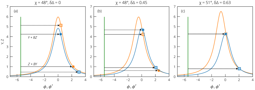
Figure 8: Graphical interpretation of asymmetric balance. Each panel shows, for different parameter values, how the symmetry broken solutions lie with respect to the resonances of the two polarization modes. Each solution is associated with two points (one for each mode, blue and orange) while the black arrows represent the corresponding (normalized) nonlinear shifts with respect to the driving laser frequency (green line at position $\phi=\phi^{\prime}=-\Delta_{+}$). Different solutions are distinguished by using respectively darker round (when the “blue” mode dominates) and lighter square (“orange” dominates) symbols, as well as solid versus dashed arrows for the nonlinear shifts. Asymmetric balance is obtained when the solutions coincide with the intersections of the two resonances. Other parameters are: $X=10.8$, $\Delta_{+}=5.45$, and $B=1.57$, as in the experiment.

The conditions in which asymmetric balance is possible can be qualitatively understood by a generalization to the asymmetric case of the diagram shown in Fig. 1(c), and that explains the origin of spontaneous symmetry breaking (SSB) in the passive nonlinear Kerr resonator. Starting from Eqs. (1)–(2), we can write the following two equations for the intracavity modal intensity levels, $Y=|E_{+}|^{2}$, $Z=|E_{-}|^{2}$, of the stationary ($\partial/\partial t=0$) solutions,

$$Y =\frac{X\cos^{2}\chi}{1+(Y+BZ-\Delta_{+})^{2}}\,,$$ (3)

$$Z =\frac{X\sin^{2}\chi}{1+(Z+BY-\Delta_{+}+\delta\Delta)^{2}}\,.$$ (4)

These equations are nonlinear and do not have closed form solutions. Their Lorentzian form, in terms of the total linear and nonlinear phase-shifts, nevertheless illustrate the resonant behaviour of the system. In the scalar case ($\chi=0^{\circ}$, $Z=0$), there exists a geometric construction of the solution to the remaining non-trivial equation, which correctly explains all the features of the scalar Kerr bistability Fraile-Peláez et al. (1991). This geometric construction cannot be generalized to the vector case above, because of the different dependence on $Y$ and $Z$ in the right-hand sides of the two equations. Using some of the ideas developed in Fraile-Peláez et al. (1991), we can however gain interesting insights about the stationary states, Eqs. (3)–(4). To this end, we plot the two resonances above, respectively versus $\phi=Y+BZ-\Delta_{+}$ and $\phi^{\prime}=Z+BY-\Delta_{+}$, along the same axis. This is illustrated for three examples in Fig. 8. Note how by construction the $Z$ resonance is shifted by $\delta\Delta$ with respect to the $Y$ resonance. The difference in amplitude on the other hand reflects the driving ellipticity $\chi$.

On these diagrams, we have represented the two symmetry-broken solutions calculated numerically for the parameters of the three examples considered. Each solution $(Y,Z)$ is plotted as a pair of points at coordinates $(\phi,Y)$ (blue) and $(\phi^{\prime},Z)$ (orange). By representing the driving laser frequency as a vertical green line at position $\phi=\phi^{\prime}=-\Delta_{+}$, the distances between that line and the different points represent the corresponding normalized nonlinear phase shifts, $Y+BZ$ (for the “blue” mode) and $Z+BY$ (for the “orange” mode). The two solutions are distinguished from each other by using respectively dark round and light square symbols as in Fig. 4, as well as with solid versus dashed arrows for the nonlinear phase shifts. We can observe that the symmetry broken solutions always lie on the right side of the resonances , where the slopes are negative, and opposite from the driving laser (green line). We remark that, in the case of scalar bistability, that side is associated with the stable upper state. Geometrically, this is explained by noting that the nonlinear phase shift has to effectively push the driving across the resonance to reach that state Fraile-Peláez et al. (1991). This correctly ties with the fact that SSB in the passive Kerr resonator always originates on the upper branch of the bistable response Haelterman et al. (1994).

In the presence of asymmetries, the two symmetry broken solutions are typically not mirror image of each other, and the points corresponding to the two solutions are distinct. This is in particular the case in presence of a single asymmetry as in Fig. 8(a), where $\chi>45^{\circ}$ (the “orange” mode is driven stronger than the “blue” mode) and $\delta\Delta=0$. Starting from that configuration, and introducing the second asymmetry by increasing $\delta\Delta$, the two resonances as plotted in our diagram can eventually intersect; see Fig. 8(b). Asymmetric balance is achieved when one symmetry broken solution matches with these intersection points [Fig. 8(c)], because at these points $Y=Z$, $\phi=\phi^{\prime}$, and each solution is the mirror image of the other. In practice, we find that this match is rarely perfect, but approaching it to within about 1 % in terms of intensities. This occurrence is nevertheless always a telltale sign that the spontaneous selection between the modes, which is the characteristic of SSB, can be restored for nearby parameters. As stable symmetry broken solutions always lie on the right side of the resonances, realizing asymmetric balance requires that the intersection points lie on that same side. Although this geometric argument cannot be turned into a simple mathematical expression at present, it can still be used to make qualitative predictions. In particular, it shows that a wavenumber difference $\delta\Delta>0$ can only be balanced when $\chi>45^{\circ}$ and vice versa. Also, a larger absolute value of $\delta\Delta$ requires $\chi$ to depart more significantly from $45^{\circ}$. Both of these trends agree with experimental observations.

References

- Anderson (1972) P. W. Anderson, More is different, Science 177, 393 (1972).
- Strocchi (2008) F. Strocchi, Symmetry Breaking (Springer, Berlin New York, 2008).
- Malomed (2013) B. A. Malomed, ed., Spontaneous Symmetry Breaking, Self-Trapping, and Josephson Oscillations, Progress in Optical Science and Photonics (Springer, Berlin Heidelberg, 2013).
- Nambu (2009) Y. Nambu, Nobel Lecture: Spontaneous symmetry breaking in particle physics: A case of cross fertilization, Rev. Mod. Phys. 81, 1015 (2009).
- Englert and Brout (1964) F. Englert and R. Brout, Broken symmetry and the mass of gauge vector mesons, Phys. Rev. Lett. 13, 321 (1964).
- Higgs (1964) P. W. Higgs, Broken symmetries and the masses of gauge bosons, Phys. Rev. Lett. 13, 508 (1964).
- Bernstein (1974) J. Bernstein, Spontaneous symmetry breaking, gauge theories, the Higgs mechanism and all that, Rev. Mod. Phys. 46, 7 (1974).
- Landau and Lifshitz (1980) L. D. Landau and E. M. Lifshitz, Statistical Physics (Elsevier, 1980).
- Tilley and Tilley (1990) D. R. Tilley and J. Tilley, Superfluidity and Superconductivity, 3rd ed., Graduate Student Series in Physics (IOP Publishing, London, 1990).
- Leggett and Sols (1991) A. J. Leggett and F. Sols, On the concept of spontaneously broken gauge symmetry in condensed matter physics, Found. Phys. 21, 353 (1991).
- Crawford and Knobloch (1991) J. D. Crawford and E. Knobloch, Symmetry and symmetry-breaking bifurcations in fluid dynamics, Annu. Rev. Fluid Mech. 23, 341 (1991).
- Turing (1952) A. M. Turing, The chemical basis of morphogenesis, Phil. Transact. Royal Soc. B 237, 37 (1952).
- Korotkevich et al. (2017) E. Korotkevich, R. Niwayama, A. Courtois, S. Friese, N. Berger, F. Buchholz, and T. Hiiragi, The apical domain is required and sufficient for the first lineage segregation in the mouse embryo, Dev. Cell 40, 235 (2017).
- Prigogine et al. (1969) I. Prigogine, R. Lefever, A. Goldbeter, and M. Herschkowitz-Kaufman, Symmetry breaking instabilities in biological systems, Nature 223, 913 (1969).
- Kaplan and Meystre (1981) A. E. Kaplan and P. Meystre, Enhancement of the Sagnac effect due to nonlinearly induced nonreciprocity, Opt. Lett. 6, 590 (1981).
- Liu et al. (2014) M. Liu, D. A. Powell, I. V. Shadrivov, M. Lapine, and Y. S. Kivshar, Spontaneous chiral symmetry breaking in metamaterials, Nature Commun. 5, 4441 (2014).
- Hamel et al. (2015) P. Hamel, S. Haddadi, F. Raineri, P. Monnier, G. Beaudoin, I. Sagnes, A. Levenson, and A. M. Yacomotti, Spontaneous mirror-symmetry breaking in coupled photonic-crystal nanolasers, Nature Photon. 9, 311 (2015).
- Cao et al. (2017) Q.-T. Cao, H. Wang, C.-H. Dong, H. Jing, R.-S. Liu, X. Chen, L. Ge, Q. Gong, and Y.-F. Xiao, Experimental demonstration of spontaneous chirality in a nonlinear microresonator, Phys. Rev. Lett. 118, 033901 (2017).
- Del Bino et al. (2017) L. Del Bino, J. M. Silver, S. L. Stebbings, and P. Del’Haye, Symmetry breaking of counter-propagating light in a nonlinear resonator, Sci. Rep. 7, 43142 (2017).
- Woodley et al. (2018) M. T. M. Woodley, J. M. Silver, L. Hill, F. Copie, L. Del Bino, S. Zhang, G.-L. Oppo, and P. Del’Haye, Universal symmetry-breaking dynamics for the Kerr interaction of counterpropagating light in dielectric ring resonators, Phys. Rev. A 98, 053863 (2018).
- Feng et al. (2014) L. Feng, Z. J. Wong, R.-M. Ma, Y. Wang, and X. Zhang, Single-mode laser by parity-time symmetry breaking, Science 346, 972 (2014).
- Hodaei et al. (2014) H. Hodaei, M.-A. Miri, M. Heinrich, D. N. Christodoulides, and M. Khajavikhan, Parity-time–symmetric microring lasers, Science 346, 975 (2014).
- Kondepudi et al. (1986) D. K. Kondepudi, F. Moss, and P. V. E. McClintock, Observation of symmetry breaking, state selection and sensitivity in a noisy electronic system, Physica D 21, 296 (1986).
- D’Angelo et al. (1992) E. J. D’Angelo, E. Izaguirre, G. B. Mindlin, G. Huyet, L. Gil, and J. R. Tredicce, Spatiotemporal dynamics of lasers in the presence of an imperfect O(2) symmetry, Phys. Rev. Lett. 68, 3702 (1992).
- Gelens et al. (2010) L. Gelens, S. Beri, G. V. der Sande, G. Verschaffelt, and J. Danckaert, Multistable and excitable behavior in semiconductor ring lasers with broken Z2-symmetry, Eur. Phys. J. D 58, 197 (2010).
- Benjamin (1978a) T. B. Benjamin, Bifurcation phenomena in steady flows of a viscous fluid. I. Theory, Proc. R. Soc. Lond. A 359, 1 (1978a).
- Benjamin (1978b) T. B. Benjamin, Bifurcation phenomena in steady flows of a viscous fluid. II. Experiments, Proc. R. Soc. Lond. A 359, 27 (1978b).
- Pipes (2003) A. Pipes, Foundations of Art and Design (Laurence King Publishing, 2003).
- Strogatz (1994) S. H. Strogatz, Nonlinear Dynamics and Chaos, Studies in Nonlinearity (Addison-Wesley, 1994).
- Hirsch et al. (1977) M. W. Hirsch, C. C. Pugh, and M. Shub, Invariant Manifolds, Lecture Notes in Mathematics, Vol. 583 (Springer-Verlag, Berlin Heidelberg New York, 1977).
- Golubitsky and Schaeffer (1979) M. Golubitsky and D. G. Schaeffer, An analysis of imperfect bifurcation, Ann. N. Y. Acad. Sci. 316, 127 (1979).
- Golubitsky and Schaeffer (1985) M. Golubitsky and D. G. Schaeffer, Singularities and Groups in Bifurcation Theory: Volume I, Applied Mathematical Sciences No. 51 (Springer-Verlag, New York, 1985).
- Ball (2001) R. Ball, Understanding critical behaviour through visualization: A walk around the pitchfork, Comput. Phys. Commun. Conference on Computational Physics 2000: "New Challenges for the New Millenium", 142, 71 (2001).
- Alam (2004) M. Alam, Universal unfolding of pitchfork bifurcations and shear-band formation in rapid granular Couette flow, arXiv:cond-mat/0411572 (2004).
- Park and Turvey (2008) H. Park and M. T. Turvey, Imperfect symmetry and the elementary coordination law, in Coordination: Neural, Behavioral and Social Dynamics, Understanding Complex Systems, edited by A. Fuchs and V. K. Jirsa (Springer, Berlin, Heidelberg, 2008) pp. 3–25.
- Ball and Brindley (2016) R. Ball and J. Brindley, The life story of Hydrogen Peroxide III: Chirality and physical effects at the dawn of life, Orig. Life Evol. Biosph. 46, 81 (2016).
- Lebreton et al. (2018) G. Lebreton, C. Géminard, F. Lapraz, S. Pyrpassopoulos, D. Cerezo, P. Spéder, E. M. Ostap, and S. Noselli, Molecular to organismal chirality is induced by the conserved myosin 1D, Science 362, 949 (2018).
- Várkonyi and Domokos (2007) P. L. Várkonyi and G. Domokos, Imperfect symmetry: A new approach to structural optima via group representation theory, Int. J. Solids Struct. 44, 4723 (2007).
- Várkonyi et al. (2006) P. L. Várkonyi, G. Meszéna, and G. Domokos, Emergence of asymmetry in evolution, Theor. Popul. Biol. 70, 63 (2006).
- Areshev et al. (1983) I. P. Areshev, T. A. Murina, N. N. Rosanov, and V. K. Subashiev, Polarization and amplitude optical multistability in a nonlinear ring cavity, Opt. Commun. 47, 414 (1983).
- Haelterman et al. (1994) M. Haelterman, S. Trillo, and S. Wabnitz, Polarization multistability and instability in a nonlinear dispersive ring cavity, J. Opt. Soc. Am. B 11, 446 (1994).
- Agrawal (2013) G. P. Agrawal, Nonlinear Fiber Optics, 5th ed. (Academic Press, 2013).
- Gilles et al. (2017) M. Gilles, P.-Y. Bony, J. Garnier, A. Picozzi, M. Guasoni, and J. Fatome, Polarization domain walls in optical fibres as topological bits for data transmission, Nature Photon. 11, 102 (2017).
- Kaplan and Meystre (1982) A. E. Kaplan and P. Meystre, Directionally asymmetrical bistability in a symmetrically pumped nonlinear ring interferometer, Opt. Commun. 40, 229 (1982).
- Lugiato and Lefever (1987) L. A. Lugiato and R. Lefever, Spatial dissipative structures in passive optical systems, Phys. Rev. Lett. 58, 2209 (1987).
- Leo et al. (2010) F. Leo, S. Coen, P. Kockaert, S.-P. Gorza, Ph. Emplit, and M. Haelterman, Temporal cavity solitons in one-dimensional Kerr media as bits in an all-optical buffer, Nature Photon. 4, 471 (2010).
- Barlow et al. (1981) A. J. Barlow, J. J. Ramskov-Hansen, and D. N. Payne, Birefringence and polarization mode-dispersion in spun single-mode fibers, Appl. Opt. 20, 2962 (1981).
- Pierce (1954) J. R. Pierce, Coupling of modes of propagation, J. Appl. Phys. 25, 179 (1954).
- Lefevre (1980) H. Lefevre, Single-mode fibre fractional wave devices and polarisation controllers, Electron. Lett. 16, 778 (1980).
- Nielsen et al. (2018) A. U. Nielsen, B. Garbin, S. Coen, S. G. Murdoch, and M. Erkintalo, Invited Article: Emission of intense resonant radiation by dispersion-managed Kerr cavity solitons, APL Photonics 3, 120804 (2018).
- Jang et al. (2013) J. K. Jang, M. Erkintalo, S. G. Murdoch, and S. Coen, Ultraweak long-range interactions of solitons observed over astronomical distances, Nature Photon. 7, 657 (2013).
- Juel et al. (1997) A. Juel, A. G. Darbyshire, and T. Mullin, The effect of noise on pitchfork and Hopf bifurcations, Proc. R. Soc. Lond. A 453, 2627 (1997).
- Garbin et al. (2017) B. Garbin, Y. Wang, S. G. Murdoch, G.-L. Oppo, S. Coen, and M. Erkintalo, Experimental and numerical investigations of switching wave dynamics in a normally dispersive fibre ring resonator, Eur. Phys. J. D 71, 240 (2017).
- (54) E. J. Doedel and B. E. Oldeman, AUTO: Continuation and bifurcation software for ordinary differential equations .
- Hodaei et al. (2017) H. Hodaei, A. U. Hassan, S. Wittek, H. Garcia-Gracia, R. El-Ganainy, D. N. Christodoulides, and M. Khajavikhan, Enhanced sensitivity at higher-order exceptional points, Nature 548, 187 (2017).
- Chen et al. (2017) W. Chen, Ş. K. Özdemir, G. Zhao, J. Wiersig, and L. Yang, Exceptional points enhance sensing in an optical microcavity, Nature 548, 192 (2017).
- Lai et al. (2019) Y.-H. Lai, Y.-K. Lu, M.-G. Suh, Z. Yuan, and K. Vahala, Observation of the exceptional-point-enhanced Sagnac effect, Nature 576, 65 (2019).
- Kominis et al. (2016) Y. Kominis, T. Bountis, and S. Flach, The asymmetric active coupler: Stable nonlinear supermodes and directed transport, Sci. Rep. 6, 33699 (2016).
- Kominis et al. (2018) Y. Kominis, K. D. Choquette, A. Bountis, and V. Kovanis, Exceptional points in two dissimilar coupled diode lasers, Appl. Phys. Lett. 113, 081103 (2018).
- Nishikawa and Motter (2016) T. Nishikawa and A. E. Motter, Symmetric states requiring system asymmetry, Phys. Rev. Lett. 117, 114101 (2016).
- Majhi et al. (2018) S. Majhi, P. Muruganandam, F. F. Ferreira, D. Ghosh, and S. K. Dana, Asymmetry in initial cluster size favors symmetry in a network of oscillators, Chaos 28, 081101 (2018).
- Hart et al. (2019) J. D. Hart, Y. Zhang, R. Roy, and A. E. Motter, Topological control of synchronization patterns: Trading symmetry for stability, Phys. Rev. Lett. 122, 058301 (2019).
- Fraile-Peláez et al. (1991) F. J. Fraile-Peláez, J. Capmany, and M. A. Muriel, Transmission bistability in a double-coupler fiber ring resonator, Opt. Lett. 16, 907 (1991).
- Note (1) This is assuming . Symmetry broken solutions of Eqs. (3)–(4) also exist for but these are always unstable, and are not considered here.