First passage time for Slepian process with linear barrier

Abstract

In this paper we extend results of L.A. Shepp by finding explicit formulas for the first passage probability $F_{a,b}(T\,|\,x)={\rm Pr}(S(t)<a+bt\text{ for all }t\in[0,T]\,\,|\,\,S(0)=x)$, for all $T>0$, where $S(t)$ is a Gaussian process with mean 0 and covariance $\mathbb{E}S(t)S(t^{\prime})=\max\{0,1-|t-t^{\prime}|\}\,.$ We then extend the results to the case of piecewise-linear barriers and outline applications to change-point detection problems. Previously, explicit formulas for $F_{a,b}(T\,|\,x)$ were known only for the cases $b=0$ (constant barrier) or $T\leq 1$ (short interval).

arXiv:0000.0000 realtime srand

,

1 Introduction

Let $T>0$ be a fixed real number and let $S(t)$, $t\in[0,T]$, be a Gaussian process with mean 0 and covariance

$$\mathbb{E}S(t)S(t^{\prime})=\max\{0,1-|t-t^{\prime}|\}\,.$$

This process is often called Slepian process and can be expressed in terms of the standard Brownian motion $W(t)$ by

$$S(t)=W(t)-W(t+1),\,\,t\geq 0.$$ (1.1)

Let $a$ and $b$ be fixed real numbers and $x<a$. We are interested in an explicit formula for the first passage probability

$$F_{a,b}(T\,|\,x):={\rm Pr}(S(t)<a+bt\text{ for all }t\in[0,T]\,\,|\,\,S(0)=x);$$ (1.2)

note $F_{a,b}(T\,|\,x)=0$ for $x\geq a$.

The case of a constant barrier, when $b=0$, has attracted significant attention in literature. In his seminal paper [1], D.Slepian has shown how to derive an explicit expression for $F_{a,0}(T\,|\,x)$ in the case $T\leq 1$; see also [2]. The case $T>1$ is much more complicated than the case $T\leq 1$. Explicit formulas for $F_{a,0}(T\,|\,x)$ with general $T$ were derived by L. A. Shepp in [3]; these formulas are special cases of results formulated in Section 2.2 and 3.1. We believe our paper can be considered as a natural extension of the methodology developed in [1] and [3]; hence the title of this paper.

In the case $T\leq 1$, Slepian’s method for deriving formulas for $F_{a,0}(T\,|\,x)$ can be easily extended to the case of a general linear barrier; see Section 7.1 for the discussion and formulas for $F_{a,b}(T\,|\,x)$ with $T\leq 1$. For general $T>0$, including the case $T>1$, explicit formulas for $F_{a,b}(T\,|\,x)$ were unknown. Derivation of these formulas is the main objective of this paper.

To do this, we generalise Shepp’s methodology of [3]. The principal distinction between Shepp’s methodology and our results is the use of an alternative way of computing coincidence probabilities. Shepp’s proofs heavily rely on the so-called Karlin-McGregor identity, see [4], but we use a different result formulated and discussed in Section 2.1.

The structure of the paper is as follows. In Section 2, we derive an expression for $F_{a,b}(T\,|\,x)$ for integer $T$ and in Section 3 we extend the results for non-integral $T$. In Sections 4 and 5, we extend the results to the case of piecewise-linear barriers. In Section 6, we outline an application to a change-point detection problem; this application was our main motivation for this research. In Appendix A, we discuss formulas for $F_{a,b}(T\,|\,x)$ with $T\leq 1$ and provide approximations for the ARL (average run length) in a change-point detection procedure. In Appendix B, we give two technical proofs.

2 Linear barrier $a+bt$ with integral $T$

In this Section, we derive an explicit formula for the first passage probability $F_{a,b}(T\,|\,x)$ defined in (1.2) under the assumption that $T$ is a positive integer, $T=n$. First, we formulate and slightly modify a general result from [5, p.40].

2.1 An important auxiliary result

Lemma 2.1.

For any $s>0$ and a positive integer $n$, let $W_{i}(t)$, $t\in[0,s]$ be $n+1$ independent Brownian Motion processes with drift parameters $\mu_{i}\in\mathbb{R}$; $i=0,1,\ldots,n$. Suppose $a_{0}<a_{1}<\ldots<a_{n}$ and $c_{0}<c_{1}<\ldots<c_{n}$ and let $dc_{0},\ldots,dc_{n}$ be infinitesimal intervals around $c_{0},\ldots,c_{n}$. Construct the vectors $\boldsymbol{\mu}=(\mu_{0},\mu_{1},\ldots,\mu_{n})^{\prime}$, $\textbf{a}=(a_{0},a_{1},\ldots,a_{n})^{\prime}$ and $\textbf{c}=(c_{0},c_{1},\ldots,c_{n})^{\prime}$. Then

$${\rm Pr}\big{\{}W_{0}(t)\!<\!W_{1}(t)\!<\!\cdots\!<\!W_{n}(t),\;\!\!\forall t\in[0,s],\!\!\;W_{i}(s)\in dc_{i}\;(0\leq i\leq n)\,\big{|}W_{i}(0)=a_{i}\;(0\leq i\leq n)\big{\}}$$ (2.1)

$$\quad\quad\quad\quad\quad\quad\quad\quad\quad=\exp\left(-\frac{s}{2}|\boldsymbol{\mu}|^{2}+\boldsymbol{\mu}\cdot(\textbf{c}-\textbf{a})\right)\det\left[\varphi_{s}({a}_{i}-{c}_{j})\right]_{i,j=0}^{n}dc_{0}dc_{1}\ldots dc_{n},\;\;\;\;\;$$

where $|\cdot|$ denotes the Euclidean norm, $\cdot$ denotes the scalar product and $\varphi_{s}(a-c)dc={\rm Pr}(W(s)\in dc\,|\,W(0)=a)$ is the transition probability for the standard Brownian Motion with no drift,

$$\varphi_{s}(z):=\frac{1}{\sqrt{2\pi s}}e^{-z^{2}/(2s)}\,.$$ (2.2)

Lemma 2.1 is an extension of the celebrated result of Karlin and McGregor on coincidence probabilities (see [4]) when applied specifically to Brownian Motion, and accommodates for different drift parameters $\mu_{i}$ of $W_{i}(t)$. Karlin-McGregor’s result can be applied to general strong Markov processes with continuous paths but no drifts. The transition probability for the process $W_{i}(t)$ is $\varphi_{s,\mu_{i}}(a-c)dc={\rm Pr}(W_{i}(s)\in dc\,|\,W_{i}(0)=a)$, where $\varphi_{s,\mu_{i}}(a-c)$ is the transition density.

Corollary 2.1.

$${\rm Pr}\left\{W_{0}(t)<W_{1}(t)<\cdots<W_{n}(t),0\leq t\leq s\,|\,W_{i}(0)=a_{i},W_{i}(s)=c_{i}\,\,(0\leq i\leq n)\right\}$$

$$\qquad\qquad\qquad=\exp\left(-\frac{s}{2}|\boldsymbol{\mu}|^{2}\!+\!\boldsymbol{\mu}\cdot(\textbf{c}-\textbf{a})\right)\det\left[\varphi_{s}({a}_{i}-{c}_{j})\right]_{i,j=0}^{n}\big{/}\prod_{i=0}^{n}\varphi_{s}({a}_{i}\!-\!{c}_{i}\!+\!{\mu}_{i}).\;\;\;$$ (2.3)

Proof. Using the relation $\varphi_{s,\mu_{i}}(a-c)=\varphi_{s}(a-(c-\mu_{i}))$ and dividing both sides of (2.1) by ${\rm Pr}(W_{i}(s)\in dc_{i},i=0,1,\ldots,n\,|\,W_{i}(0)=a_{i},i=0,1,\ldots,n)$, we obtain the result.

$\Box$

2.2 The main result

Let $\varphi(t)=\varphi_{1}(t)$ and $\Phi(t)=\int_{-\infty}^{t}\varphi(u)du$ be the density and the c.d.f. of the standard normal distribution. Assume that $T=n$ is a positive integer. Define $(n\!+\!1)$-dimensional vectors

$$\boldsymbol{\mu}=\begin{bmatrix}0\\ b\\ 2b\\ \vdots\\ nb\end{bmatrix},\;\;\textbf{a}=\begin{bmatrix}0\\ x_{1}\!+\!a\\ x_{2}\!+\!2a\!+\!b\\ \vdots\\ x_{n}\!+\!na\!+\!\frac{(n-1)n}{2}b\end{bmatrix},\;\;\textbf{c}=\begin{bmatrix}x_{1}\\ x_{2}\!+\!a\!+\!b\\ x_{3}\!+\!2a\!+\!3b\\ \vdots\\ x_{n+1}\!+\!(a\!+\!b)n\!+\!\frac{(n-1)n}{2}b\end{bmatrix}$$ (2.4)

and let ${\mu}_{i}$, ${a}_{i}$ and ${c}_{i}$ be $i$-th components of vectors $\boldsymbol{\mu}$, a and c respectively ($i=0,1,\ldots,n$). Note that we start the indexation of vector components at 0.

Theorem 2.1.

For any integer $n\geq 1$ and $x<a$,

$$\qquad F_{a,b}(n\,|\,x)\!=\!\frac{1}{\varphi(x)}\int_{-x-a-b}^{\infty}\int_{x_{2}-a-2b}^{\infty}\!\!\!\!\!\!\!\!\! \!\!\ldots\int_{x_{n}-a-nb}^{\infty}\exp(-|\boldsymbol{\mu}|^{2}/2+\boldsymbol{\mu}\cdot(\textbf{c}-\textbf{a}))$$ (2.5)

$$\qquad\quad\times\det\left[\varphi({a}_{i}-{c}_{j})\right]_{i,j=0}^{n}\,dx_{n+1}\,dx_{n}\!\ldots\,dx_{2}\,,\;\;\;\;$$

where $\boldsymbol{\mu}$, a and c are given in (2.4).

If $b=0$ then (2.5) coincides with Shepp’s formula (2.15) in [3] expressed in variables $y_{i}=x_{i}+ia$ ($i=0,1,\ldots,n$).

In the case $T=2$ we obtain

$$F_{a,b}(2\,|\,x)\!\!\!\! = \!\!\!\!\frac{e^{5b^{2}/2+bx}}{\varphi(x)}\int_{-x-a-b}^{\infty}\int_{x_{2}-a-2b}^{\infty}e^{b(2x_{3}-x_{2})}$$

$$\times \!\!\!\!\det\begin{bmatrix}\varphi(x)&\varphi(-x_{2}\!-\!a\!-\!b)&\varphi(-x_{3}\!-\!2a\!-\!3b)\\ \varphi(a)&\varphi(-x\!-\!x_{2}\!-\!b)&\varphi(-x\!-\!a\!-\!x_{3}\!-\!3b)\\ \varphi(x_{2}\!+\!2a\!+\!b\!+\!x)&\varphi(a)&\varphi(x_{2}\!-\!x_{3}\!-\!2b)\\ \end{bmatrix}dx_{3}dx_{2}.$$

2.3 An alternative representation of formula (2.5) and two particular cases

It is easier to interpret Theorem 2.1 by expressing the integrals in terms of the values of $S(t)$ at times $t=0,1,\ldots,n$. Let $x_{0}=0,x_{1}=-x.$ For $i=0,1,\ldots,n$ we set $s_{i}=x_{i}-x_{i+1}$ with $s_{0}=x$. It follows from the proof of (2.5), see Section 2.4, that $s_{0},s_{1},\ldots,s_{n}$ have the meaning of the values of the process $S(t)$ at times $t=0,1,\ldots,n$; that is, $S(i)=s_{i}$ ($i=0,1,\ldots,n$). The range of the variables $s_{i}$ in (2.5) is $(-\infty,a+bi)$, for $i=0,1,\ldots,n$ . The variables $x_{1},\ldots,x_{n+1}$ are expressed via $s_{0},\ldots,s_{n}$ by $x_{k}=-s_{0}-s_{1}-\ldots-s_{k-1}$ ($k=1,\ldots,n+1$) with $x_{0}=0$. Changing the variables, we obtain the following equivalent expression for the probability $F_{a,b}(n\,|\,x)$:

$$F_{a,b}(n\,|\,x)\!=\!\frac{1}{\varphi(x)}\int_{-\infty}^{a+b}\int_{-\infty}^{a+2b} \!\!\!\!\!\!\!\!\!\!\!\cdots\int_{-\infty}^{a+bn}\exp(-|\boldsymbol{\mu}|^{2}/2+\boldsymbol{\mu}\cdot(\textbf{c}-\textbf{a}))$$

$$\qquad\!\!\times\det\left[\varphi({a}_{i}-{c}_{j})\right]_{i,j=0}^{n}\,ds_{n}\!\ldots ds_{2}ds_{1}\,,$$

where $\boldsymbol{\mu}$ is given by (2.4) but expressions for a and c change:

$$\textbf{a}=\begin{bmatrix}0\\ \!a\!-\!s_{0}\\ 2a\!+\!b\!-\!s_{0}\!-\!s_{1}\\ \vdots\\ na\!+\!\frac{(n-1)n}{2}b\!-\!s_{0}\!-\!s_{1}\!-\!\ldots\!-\!s_{n-1}\end{bmatrix}\!,\;\;\textbf{c}=\begin{bmatrix}-s_{0}\\ a\!+\!b\!-\!s_{0}\!-\!s_{1}\\ 2a\!+\!3b\!-\!s_{0}\!-\!s_{1}\!-\!s_{2}\\ \vdots\\ (a\!+\!b)n\!+\!\frac{(n-1)n}{2}b\!-\!s_{0}\!-\!s_{1}\!-\!\ldots\!-\!s_{n}\end{bmatrix}.\;\;\;\;$$

In a particular case of $n=1$ we obtain:

$$\quad F_{a,b}(1\,|\,x)\!\!\!\! = \!\!\!\!\frac{1}{\varphi(x)}\int_{-\infty}^{a+b}\exp(-b^{2}/2\!+\!b(b-s_{1}))\det\begin{bmatrix}\varphi(x)&\varphi(x+s_{1}-a-b)\\ \varphi(a)&\varphi(s_{1}-b)\\ \end{bmatrix}ds_{1}$$ (2.6)

$$= \!\!\!\!\Phi(a+b)-\exp\left(-(a^{2}-x^{2})/2-b(a-x)\right)\Phi(x+b),$$

which agrees with (7.1) in the Appendix A. For the case of $n=2$ we obtain:

$$F_{a,b}(2\,|\,x)\!\!\!\! = \!\!\!\!\frac{e^{5b^{2}\!/\!2}}{\varphi(x)}\int_{-\infty}^{a\!+\!b}\!\int_{-\infty}^{a\!+\!2b}e^{-b(s_{1}\!+\!2s_{2})}$$

$$\times \!\!\!\!\det\!\!\begin{bmatrix}\varphi(x)\!\!\!&\!\!\!\varphi(x\!\!+\!\!s_{1}\!\!-\!\!a\!\!-\!\!b)&\varphi(x\!\!+\!\!s_{1}\!\!+\!\!s_{2}\!\!-\!\!2a\!\!-\!\!3b)\\ \varphi(a)\!\!\!&\!\!\varphi(s_{1}-b)&\varphi(s_{1}+s_{2}-a-3b)\\ \varphi(2a\!+\!b\!-\!s_{1})\!\!\!&\varphi(a)&\varphi(s_{2}-2b)\\ \end{bmatrix}\!\!ds_{2}ds_{1}.$$

2.4 Proof of Theorem 2.1

Using (1.1) we rewrite $F_{a,b}(n\,|\,x)$ as

$$F_{a,b}(n\,|\,x)\!\!\!\! = \!\!\!\!{\rm Pr}\{W(t)\!-\!W(t\!+\!1)\!<a\!+\!bt\text{ for all }t\!\in\![0,n]\,\,|\,\,W(0)\!-\!W(1)\!=\!x\}$$

$$= \!\!\!\!{\rm Pr}\{W(t)\!-\!W(t\!+\!1)<a+bt,\,\,W(t\!+\!1)\!-\!W(t\!+\!2)<\!a+b(t\!+\!1),\ldots,$$

$$\quad\!W(t\!+\!n\!-\!1)\!-\!W(t\!+\!n)\!<\!a\!+\!b(t+\!n\!-1)\text{ for all }t\!\in\![0,1]\,\,\big{\lvert}\,\,W(0)\!-\!W(1)\!=\!x\}$$

$$= \!\!\!\!{\rm Pr}\bigg{\{}W(t)\!<\!W(t\!+\!1)\!+\!a\!+\!bt<\!\cdots\!<W(t\!+\!n)\!+\!n(a\!+\!bt)\!+\!\frac{(n\!-\!1)n}{2}b$$

$$\quad\text{for all }t\!\in\![0,1]\,\,|\,\,W(0)\!-\!W(1)\!=\!x\bigg{\}}.$$

Let $\Omega$ be the event defined as follows

$$\Omega=\left\{W(t)\!<\!W(t\!+\!1)\!+\!a\!+\!bt<\!\cdots\!<W(t\!+\!n)\!+\!n(a\!+\!bt)\!+\!\frac{(n\!-\!1)n}{2}b\text{ for all }t\!\in\![0,1]\right\}$$

and let $x_{i}=W(i)$, $i=0,1,\ldots,n\!+\!1$. Integrating out over the values $x_{i}$, by the law of total probability we obtain:

$$\qquad F_{a,b}(n\,|\,x)\!=\!\int\!\!\!\!\!\! \cdots \!\!\!\!\!\!\int{\rm Pr}\{\Omega\,\,|\,\,W(0)\!=\!x_{0},\ldots,W(n\!+\!1)\!=\!x_{n+1},W(0)\!-\!W(1)\!=\!x\}$$ (2.7)

$$\!\!\!\!\times\,{\rm Pr}\{W(0)\!\in\!dx_{0},\ldots,W(n\!+\!1)\!\in\!dx_{n+1}\,|\,W(0)\!-\!W(1)\!=\!x\}.$$

Note that $W(1)=x_{1}=-x$, since $W(0)-W(1)=x$ and $W(0)=0$. For $i=0,1,\ldots,n$, define the processes

$$W_{i}(t)=W(t+i)+i(a+bt)+\frac{(i-1)i}{2}b,\,\,\,\,0\leq t\leq 1.$$

Then the event $\Omega$ above can be equivalently expressed as

$$\Omega=\{W_{0}(t)<W_{1}(t)<\cdots<W_{n}(t)\text{ for all }t\in[0,1]\}$$ (2.8)

and under the conditioning introduced in (2.7), we have for $i=0,1,\ldots,n$:

$$W_{i}(0)\!\!\! = \!\!\!W(i)+ia+\frac{(i-1)i}{2}b=x_{i}+ia+\frac{(i-1)i}{2}b\,,$$

$$W_{i}(1)\!\!\! = \!\!\!W(i+1)+i(a+b)+\frac{(i-1)i}{2}b=x_{i+1}+i(a+b)+\frac{(i-1)i}{2}b\,.$$

Therefore (2.7) can expressed as

$$F_{a,b}(n\,|\,x)\!=\!\!\int\!\!\cdots\!\!\!\!\int\!{\rm Pr}\bigg{\{}\Omega\,\big{|}\,W_{i}(0)\!=\!x_{i}\!+\!ia\!+\!\frac{(i\!-\!1)i}{2}b,\;W_{i}(1)\!=\!x_{i+1}\!+\!i(a\!+\!b)\!+\!\frac{(i\!-\!1)i}{2}b\;(0\leq i\leq n),$$

$$W_{0}(0)\!-\!W_{0}(1)\!=\!x\!\bigg{\}}\;{\rm Pr}\{W(0)\!\in\!dx_{0},\ldots,\!W(n\!+\!1)\!\in\!dx_{n+1}\!\,|\,W(0)\!-\!W(1)\!=\!x\}.\;\;\;\;\;\;\;\;\;\;\;\;\;\;\;\;\;\;$$ (2.9)

The region of integration for (2.4) is determined from the following chain of inequalities which ensure that the inequalities in (2.8) hold at $t=0$ and $t=1$:

$$x_{1}<x_{2}\!+\!a\!+\!b<\ldots<x_{n}\!+\!(n-1)(a\!+\!b)\!+\!\frac{(n\!-\!2)(n\!-\!1)}{2}b<x_{n+1}\!+\!n(a\!+\!b)\!+\!\frac{(n\!-\!1)n}{2}b\,.$$

Hence, the upper limit of integration for all variables is infinity and the lower limit for the integral with respect to $x_{i+1}$, $i=1,\ldots,n$, is given by the formula:

$$x_{i}+(i-1)(a+b)+\frac{(i-2)(i-1)}{2}b-i(a+b)-\frac{(i-1)i}{2}b=x_{i}-a-b-(i-1)b\,.$$

Since the conditioned Brownian Motion processes $W_{i}(t)$ are independent, using (2.1) we can express the first term in (2.4) as

$${\rm Pr}\bigg{\{}\!\Omega\,\big{|}\,W_{i}(0)\!\!\!\! = \!\!\!x_{i}\!+\!ia\!+\!\frac{(i\!-\!1)i}{2}b,W_{i}(1)\!=\!x_{i+1}\!+\!i(a\!+\!b)\!+\!\frac{(i\!-\!1)i}{2}b\text{ for }i=0,1,\ldots n\bigg{\}}$$

$$= \!\!\!\exp(-|\boldsymbol{\mu}|^{2}/2+\boldsymbol{\mu}\cdot(\textbf{c}-\textbf{a}))\det\left[\varphi({a}_{i}-{c}_{j})\right]_{i,j=0}^{n}\big{/}\prod_{i=0}^{n}\varphi({a}_{i}-{c}_{i}+{\mu}_{i}),$$

where $\boldsymbol{\mu}$, a and c are defined in (2.4). The second probability in the right hand side of (2.4) is simply $\prod_{i=1}^{n}\varphi(x_{i}-x_{i+1})$. By noticing

$$\prod_{i=0}^{n}\varphi({a}_{i}-{c}_{i}+{\mu}_{i})=\prod_{i=0}^{n}\varphi(x_{i}-x_{i+1}-ib+{\mu}_{i})=\prod_{i=0}^{n}\varphi(x_{i}-x_{i+1})$$

and collating all terms, we obtain (2.5). $\Box$

3 Linear barrier $a+bt$ with non-integral $T$

In this section, we shall derive an explicit formula for the first passage probability $F_{a,b}(T\,|\,x)$ defined in (1.2) assuming $T>0$ is not an integer. Represent $T$ as $T=m+\theta$, where $m=\lfloor T\rfloor\geq 0$ is the integer part of $T$ and $0<\theta<1$. Set $n=m+1=\lceil T\rceil$.

3.1 The main result

Let $\varphi_{\theta}(t)$ and $\varphi_{1-\theta}(t)$ be as defined in (2.2). Define the $(n\!+\!1)$- and $n$-dimensional vectors as follows: $\boldsymbol{\mu}_{1}=\boldsymbol{\mu}$ is as defined in (2.4),

$${\textbf{a}_{1}}=\begin{bmatrix}0\\ u_{1}\!+\!a\\ u_{2}\!+\!2a\!+\!b\\ \vdots\\ u_{n}\!+\!na\!+\!\frac{n(n-1)}{2}b\end{bmatrix},\;\;\textbf{c}_{1}=\begin{bmatrix}v_{0}\\ v_{1}\!+\!a\!+\!b\theta\\ v_{2}\!+\!2(a\!+\!b\theta)\!+\!b\\ \vdots\\ v_{n}\!+\!n(a\!+\!b\theta)\!+\!\frac{n(n-1)}{2}b\end{bmatrix},$$ (3.1)

$$\boldsymbol{\mu}_{2}=\begin{bmatrix}0\\ b\\ 2b\\ \vdots\\ mb\end{bmatrix},\;\textbf{a}_{2}=\begin{bmatrix}v_{0}\\ v_{1}\!+\!a\!+\!b\theta\\ v_{2}\!+\!2(a\!+\!b\theta)\!+\!b\\ \vdots\\ v_{m}\!+\!m(a\!+\!b\theta)\!+\!\frac{(m-1)m}{2}b\end{bmatrix},\;\textbf{c}_{2}=\begin{bmatrix}u_{1}\\ u_{2}\!+\!a\!+\!b\\ u_{3}\!+\!2a\!+\!3b\\ \vdots\\ u_{m+1}\!+\!m(a\!+\!b)\!+\!\frac{(m-1)m}{2}b\end{bmatrix},$$

and let ${{a}_{1}}_{i}$ and ${{c}_{1}}_{i}$ be $i$-th components of vectors $\textbf{a}_{1}$ and $\textbf{c}_{1}$ respectively ($i\!=\!0,1,\ldots,n$). Similarly, let ${{a}_{2}}_{i}$ and ${{c}_{2}}_{i}$ be $i$-th components of vectors $\textbf{a}_{2}$ and $\textbf{c}_{2}$ respectively ($i\!=\!0,1,\ldots,m$). Recall that we start the indexation of vector components at 0.

Theorem 3.1.

For $x<a$ and non-integral $T=m+\theta$ with $0<\theta<1$, we have

$$F_{a,b}(T\,|\,x)\!\!\!\!\! = \!\!\!\!\!\frac{1}{\varphi(x)}\int_{-x-a-b}^{\infty}\!\cdots\!\int_{u_{m}-a-mb}^{\infty}\int_{-\infty}^{\infty}\int_{v_{0}-a-b\theta}^{\infty}\!\cdots\int_{v_{m}-a-b\theta-mb}^{\infty}$$

$$\!\!\!\exp(-\theta|\boldsymbol{\mu}_{1}|^{2}/2+\boldsymbol{\mu}_{1}\cdot(\textbf{c}_{1}-\textbf{a}_{1}))\exp(-(1\!-\!\theta)|\boldsymbol{\mu}_{2}|^{2}/2+\boldsymbol{\mu}_{2}\cdot(\textbf{c}_{2}-\textbf{a}_{2}))$$

$$\!\!\!\det[\varphi_{\theta}({{a}_{1}}_{i}-{{c}_{1}}_{j})]_{i,j=0}^{n}\det[\varphi_{1-\theta}({{a}_{2}}_{i}-{{c}_{2}}_{j})]_{i,j=0}^{m}\,\,dv_{m+1}\ldots dv_{1}dv_{0}du_{m+1}\ldots du_{2}\,.$$

Proof is given below in Section 3.3.

If $b=0$ then the above formula for $F_{a,b}(T\,|\,x)$ coincides with Shepp’s formula (2.25) in [3] expressed in variables $x_{i}=u_{i}+ia$ and $y_{i}=v_{i}+ia$ ($i=0,1,\ldots,n$).

3.2 Two particular cases of Theorem 3.1

Taking $m=0$ and hence $T=\theta$ yields the following

$$F_{a,b}(\theta\,|\,x)\!\!\! = \!\!\!\frac{e^{\theta b^{2}/2}}{\varphi(x)}\int_{-\infty}^{\infty}\int_{v_{0}-a-b\theta}^{\infty}e^{b(v_{1}+x)}\varphi_{1-\theta}(v_{0}\!+\!x)$$

$$\times \!\!\det\begin{bmatrix}\varphi_{\theta}(\!-v_{0})&\varphi_{\theta}(-v_{1}\!-\!a\!-\!b\theta)\\ \varphi_{\theta}(-x\!+\!a\!-\!v_{0})\!\!\!\!\!&\varphi_{\theta}(-x\!-\!v_{1}\!-\!b\theta)\\ \end{bmatrix}dv_{1}dv_{0}$$

which agrees numerically with (7.1) in the Appendix for $T<1$. Taking $T=1+\theta$ yields

$$F_{a,b}(1\!+\!\theta\,|\,x)\!\!\!\!\! = \!\!\!\!\!\frac{1}{\varphi(x)}\int_{-x-a-b}^{\infty}\int_{-\infty}^{\infty}\int_{v_{0}-a-b\theta}^{\infty}\int_{v_{1}-a-b\theta-b}^{\infty}\!\!\exp(-(1\!-\!\theta)b^{2}/2\!+\!b(u_{2}\!-\!v_{1}\!+\!b(1\!-\!\theta))$$

$$\times \!\!\!\!\exp(-\theta(b^{2}\!+\!4b^{2})/2\!+\!b(v_{1}\!+\!b\theta\!+\!x)+\!2b(v_{2}\!-\!u_{2}\!+\!2b\theta))$$

$$\times \!\!\!\!\det\begin{bmatrix}\varphi_{1-\theta}(v_{0}\!+\!x)&\varphi_{1-\theta}(v_{0}\!-\!u_{2}\!-\!a\!-\!b)\\ \varphi_{1-\theta}(v_{1}\!+\!a\!+\!b\theta\!+\!x)&\varphi_{1-\theta}(v_{1}\!-\!u_{2}\!-\!b(1\!-\!\theta))\\ \end{bmatrix}$$

$$\times \!\!\!\!\det\begin{bmatrix}\varphi_{\theta}(\!-v_{0})&\varphi_{\theta}(-v_{1}\!-\!a\!-\!b\theta)&\varphi_{\theta}(-v_{2}\!-\!2(a\!+\!b\theta)\!-\!b)\\ \varphi_{\theta}(-x\!+\!a\!-\!v_{0})&\varphi_{\theta}(-x\!-\!v_{1}\!-\!b\theta)&\varphi_{\theta}(-x\!-\!v_{2}\!-\!a\!-\!b(1\!+\!2\theta))\\ \varphi_{\theta}(u_{2}\!+\!2a\!+\!b\!-\!v_{0})\!\!\!&\varphi_{\theta}(u_{2}\!-\!v_{1}\!+\!a\!+\!b(1\!-\!\theta))\!\!\!\!\!&\varphi_{\theta}(u_{2}\!-\!v_{2}\!-\!2b\theta)\\ \end{bmatrix}$$

$$\qquad\qquad\qquad\qquad\qquad\qquad\qquad\qquad\qquad\qquad\qquad\qquad\qquad dv_{2}dv_{1}dv_{0}du_{2}\,.$$

3.3 Proof of Theorem 3.1

We are interested in an expression for the first passage probability

$$F_{a,b}(T\,|\,x)={\rm Pr}(S(t)<a+bt\text{ for all }t\in[0,m+\theta]\,\,|\,\,S(0)=x).$$

Using (1.1), $F_{a,b}(T\,|\,x)$ can be equivalently expressed as follows

$$F_{a,b}(T\,|\,x)\!\!\!\!\! = \!\!\!\!{\rm Pr}\{W(t)\!-\!W(t\!+\!1)\!<\!a\!+\!bt\text{ for all }t\!\in\![0,m+\theta]\,\,|\,\,W(0)\!-\!W(1)\!=\!x\}$$

$$= \!\!\!\!{\rm Pr}\bigg{\{}W(t)\!<\!W(t\!+\!1)\!+\!a\!+\!bt\!<\!\ldots\!<\!W(t\!+\!m\!+\!1)\!+\!(m\!+\!1)(a\!+\!bt)\!+\!\frac{(m\!+\!1)m}{2}b$$

$$\quad\text{for all }t\!\in\![0,\theta]\text{ and }W(\tau\!+\!\theta)\!<\!W(\tau\!+\!\theta\!+\!1)\!+\!a\!+\!b\theta\!+\!b\tau\!<\!\ldots\!<\!$$

$$\quad W(\tau\!+\!\theta\!+\!m)+\!m(a\!+\!b\theta\!+\!b\tau)\!+\!\frac{(m\!-\!1)m}{2}b\text{ for all }\tau\!\in\![0,1-\theta]|\,W(0)\!-\!W(1)\!=\!x\bigg{\}}.$$

Let $\Omega$ be the event

$$\Omega\! = \!\bigg{\{}W(t)\!<\!W(t\!+\!1)\!+\!a\!+\!bt\!<\!\ldots\!<\!W(t\!+\!m\!+\!1)\!+\!(m\!+\!1)(a\!+\!bt)\!+\!\frac{(m\!+\!1)m}{2}b$$

$$\quad\!\text{for all }t\!\in\![0,\theta]\text{ and }W(\tau\!+\!\theta)\!<\!W(\tau\!+\!\theta\!+\!1)\!+\!a\!+\!b\theta\!+\!b\tau\!<\!\ldots\!<\!W(\tau\!+\!\theta\!+\!m)+$$

$$\quad\!m(a\!+\!b\theta\!+\!b\tau)+\frac{(m\!-\!1)m}{2}b\text{ for all }\tau\!\in\![0,1-\theta]\bigg{\}}.$$

Then by integrating out over the values $u_{i}$ and $v_{i}$ of $W$ at times $i$ and $i+\theta$, $i=0,1,\ldots,m+\!1$, by the law of total probability we have

$$F_{a,b}(T\,|\,x)=\!\int\!\!\!\!\! \cdots \!\!\!\!\!\int\!{\rm Pr}\{\Omega\,\big{|}\,W(0)\!=\!u_{0},\ldots,\!W(m\!+\!1)\!=\!u_{m+1},W(\theta)\!=\!v_{0},\ldots,\!$$ (3.3)

$$\qquad\!\!W(m\!+\!1\!+\!\theta)\!=\!v_{m+1},W(0)\!-W(1)\!=\!x\}\times$$

$$\,{\rm Pr}\{W(0)\!\in\!du_{0},\ldots,\!W(m\!+\!1)\!\in\!du_{m+1},W(\theta)\!\in\!dv_{0},\ldots,$$

$$\qquad\!\!\!W(m\!+\!1\!+\!\theta)\!\in\!dv_{m+1}\,|\,W(0)\!-\!W(1)\!=\!x\}.$$

Note that $W(1)=x_{1}=-x$, since $W(0)-W(1)=x$ and $W(0)=0$, and define the processes

$$W_{i}(t) = W(t+i)+i(a+bt)+\frac{(i-1)i}{2}b,\,\,\,\,0\leq t\leq\theta,\,\,\,\,i=0,1,\ldots,m+1\,,$$

$$W_{j}^{\prime}(t) = W(\tau+\theta+j)+j(a+b\theta+b\tau)+\frac{(j-1)j}{2}b,\,\,\,\,0\leq\tau\leq 1-\theta,\,\,\,\,j=0,1,\ldots,m\,.$$

Then the event $\Omega$ can be equivalently expressed as $\Omega=\Omega_{1}\cap\Omega_{2}$ with

$$\Omega_{1}\!\!\! = \!\!\!\{W_{0}(t)<W_{1}(t)<\cdots<W_{m+1}(t)\text{ for all }t\in[0,\theta]\},$$

$$\Omega_{2}\!\!\! = \!\!\!\{W_{0}^{\prime}(\tau)<W_{1}^{\prime}(\tau)<\cdots<W_{m}^{\prime}(\tau)\text{ for all }\tau\in[0,1-\theta]\}.$$

Under the conditioning introduced in (3.3) we have for $i\!=\!0,1,\ldots,m+1$ and $j\!=\!0,1,\ldots,m$:

$$W_{i}(0)\!\!\! = \!\!\!W(i)+ia+\frac{(i-1)i}{2}b=u_{i}+ia+\frac{(i-1)i}{2}b\,,$$

$$W_{i}(\theta)\!\!\! = \!\!\!W(i+\theta)+i(a+b\theta)+\frac{(i-1)i}{2}b=v_{i}+i(a+b\theta)+\frac{(i-1)i}{2}b\,,$$

$$W_{j}^{\prime}(0)\!\!\! = \!\!\!W(j+\theta)+j(a+b\theta)+\frac{(j-1)j}{2}b=v_{j}+j(a+b\theta)+\frac{(j-1)j}{2}b\,,$$

$$W_{j}^{\prime}(1-\theta)\!\!\! = \!\!\!W(j+1)+j(a+b)+\frac{(j-1)j}{2}b=u_{j+1}+j(a+b)+\frac{(j-1)j}{2}b\,.$$

Now under the above conditioning the processes are independent and so the conditional probability of $\Omega$ in (3.3) becomes a product of the conditional probabilities of $\Omega_{1}$ and $\Omega_{2}$. Therefore, (3.3) becomes

$$F_{a,b}(T\,|\,x)\!=\!\!\int\!\!\!\!\! \cdots \!\!\!\!\!\int\!{\rm Pr}\bigg{\{}\!\Omega_{1}\,\big{|}\,W_{i}(0)\!=\!u_{i}\!+\!ia\!+\!\frac{(i\!-\!1)i}{2}b,W_{i}(\theta)\!=\!v_{i}\!+\!i(a\!+\!b\theta)\!+\!\frac{(i\!-\!1)i}{2}b,$$ (3.4)

$$\qquad(0\!\leq\!i\!\leq\!m\!+\!1)\bigg{\}}\times{\rm Pr}\bigg{\{}\!\Omega_{2}\,\big{|}\,W_{j}^{\prime}(0)\!=\!v_{j}\!+\!j(a\!+\!b\theta)\!+\!\frac{(j\!-\!1)j}{2}b,$$

$$\qquad W_{j}^{\prime}(1\!-\!\theta)\!=\!u_{j+1}\!+\!j(a\!+\!b)\!+\!\frac{(j\!-\!1)j}{2}b\,\,(0\!\leq\!j\leq\!m)\bigg{\}}\!\!\times\!{\rm Pr}\{W(0)\!\in\!du_{0}$$

$$\qquad,\ldots,W(m\!+\!1)\!\in\!du_{m+1},W(\theta)\!\in\!dv_{0},\ldots,W(m\!+\!1\!+\!\theta)\!\in\!dv_{m+1}$$

$$\qquad|W(0)\!-\!W(1)\!=\!x\}.$$

The region of integration for the variables $u_{i}$ in (3.4) is determined from the following chain of inequalities:

$$-x-a<u_{2}+2a+b<\ldots<u_{m}+ma+\frac{(m-1)m}{2}b<u_{m+1}+(m+1)a+\frac{(m+1)m}{2}b\,.$$

Whence, the upper limit of integration with respect to $u_{i+1}$ is infinity and the lower limit for the integral with respect to $u_{i+1}$, $i=1,\ldots,m$ is given by the formula $u_{i}-a-ib$. For the variables $v_{j}$ in (3.4), we have the following chain of inequalities

$$v_{0}<v_{1}\!+\!a\!+\!b\theta\!<\ldots\!<v_{m}\!+\!m(a+b\theta)\!+\!\frac{(m-1)m}{2}b<v_{m+1}\!+\!(m+1)(a+b\theta)\!+\!\frac{(m+1)m}{2}b\,.$$

Once again, the upper limit of integration with respect to $v_{i+1}$ is infinity and the lower limit for the integral with respect to $v_{i+1}$ ($i=0,\ldots,m$) is $v_{i}-a-b\theta-ib$. For $v_{0}$, the upper and lower limits of integration are infinite.

Now using (2.1) with $n=m+1$ we obtain

$$\!\!{\rm Pr}\bigg{\{}\!\Omega_{1}\,\big{|}\,W_{i}(0)\!\!=\!\!u_{i}\!+\!ia\!+\!\frac{(i\!-\!1)i}{2}b,W_{i}(\theta)\!=\!v_{i}\!+\!i(a\!+\!b\theta)\!+\!\frac{(i\!-\!1)i}{2}b,\,\,(0\leq i\leq m\!+\!1)\bigg{\}}$$

$$\qquad=\exp(-\theta|\boldsymbol{\mu}_{1}|^{2}/2+\boldsymbol{\mu}_{1}\cdot(\textbf{c}_{1}-\textbf{a}_{1}))\det[\varphi_{\theta}({{a}_{1}}_{i}-{{c}_{1}}_{j})]_{i,j=0}^{m+1}\,\big{/}\prod_{i=0}^{m+1}\varphi_{\theta}({{a}_{1}}_{i}-{{c}_{1}}_{i}+\theta{{\mu}_{1}}_{i}),$$

where $\varphi_{\theta}(\cdot)$ is given in (2.2), ${\textbf{a}_{1}}$ and ${\textbf{c}_{1}}$ are given in (3.1). Similarly, using (2.1) with $n=m$ we have

$$\!\!\!\!{\rm Pr}\bigg{\{}\!\Omega_{2}\,\big{|}\,W_{j}^{\prime}(0)\!=\!v_{j}\!+\!j(a\!+\!b\theta)\!+\!\frac{(j\!-\!1)j}{2}b,W_{j}^{\prime}(1\!-\!\theta)\!=\!u_{j+1}\!+\!j(a\!+\!b)\!+\!\frac{(j\!-\!1)j}{2}b,(0\!\leq\!j\!\leq\!m)\!\bigg{\}}$$

$$\qquad=\exp(-(1\!-\!\theta)|\boldsymbol{\mu}_{2}|^{2}/2+\boldsymbol{\mu}_{2}\cdot(\textbf{c}_{2}-\textbf{a}_{2}))\det[\varphi_{1-\theta}({{a}_{2}}_{i}-{{c}_{2}}_{j})]_{i,j=0}^{m}$$

$$\qquad\qquad\qquad\qquad\qquad\qquad\qquad\qquad\big{/}\prod_{i=0}^{m}\varphi_{1-\theta}({{a}_{2}}_{i}\!-\!{{c}_{2}}_{i}+(1\!-\!\theta){{\mu}_{2}}_{i}),$$

where $\varphi_{1-\theta}(\cdot)$ is given in (2.2), ${\textbf{a}_{2}}$ and ${\textbf{c}_{2}}$ are given in (LABEL:bzy_2). The third probability in the right-hand side of (3.4) is simply

$$\frac{1}{\varphi(x)}\prod_{j=0}^{m}\prod_{i=0}^{m+1}\varphi_{\theta}(u_{i}-v_{i})\varphi_{1-\theta}(v_{j}-u_{j+1})\,.$$

By noticing

$$\prod_{j=0}^{m}\prod_{i=0}^{m+1}\varphi_{\theta}({{a}_{1}}_{i}\!-\!{{c}_{1}}_{i}+\theta{{\mu}_{1}}_{i})\varphi_{1-\theta}({{a}_{2}}_{j}\!-\!{{c}_{2}}_{j}\!+\!(1\!-\!\theta){{\mu}_{2}}_{j})=\prod_{j=0}^{m}\prod_{i=0}^{m+1}\varphi_{\theta}(u_{i}\!-\!v_{i})\varphi_{1-\theta}(v_{j}\!-\!u_{j+1})$$

and collating all terms, we obtain the result. $\Box$

4 Piecewise linear barrier with one change of slope

4.1 Formulation of the main result

In this section, we derive an explicit formula for the first passage probability for $S(t)$ with a continuous piecewise linear barrier, where not more than one change of slope is allowed. For any non-negative $T,T^{\prime}$ and real $a,b,b^{\prime}$ we define the piecewise-linear barrier $B_{T,T^{\prime}}(t;a,b,b^{\prime})$ by

$$B_{T,T^{\prime}}(t;a,b,b^{\prime})=\begin{cases}a+bt&t\in[0,T],\\ a+bT+b^{\prime}(t-T)&t\in[T,T+T^{\prime}]\,;\end{cases}$$

for an illustration of this barrier, see Figure 1. We are interested in finding an expression for the first passage probability

$$\qquad\qquad F_{a,b,b^{\prime}}(T,T^{\prime}\,|\,x):={\rm Pr}(S(t)<B_{T,T^{\prime}}(t;a,b,b^{\prime})\text{ for all }t\in[0,T+T^{\prime}]\,\,|\,\,S(0)=x).$$ (4.1)

We only consider the case when both $T$ and $T^{\prime}$ are integers. The case of general $T,T^{\prime}$ can be treated similarly but the resulting expressions are much more complicated.

Figure 1: Graphical depiction of a general boundary $B_{T,T^{\prime}}(t;a,b,b^{\prime})$ with negative $b$ and positive $b^{\prime}$.

Define the $(T+T^{\prime}\!+\!1)$-dimensional vectors as follows:

$$\boldsymbol{\mu}_{3}=\begin{bmatrix}0\\ b\\ 2b\\ \vdots\\ Tb\\ b^{\prime}+Tb\\ 2b^{\prime}+Tb\\ \vdots\\ T^{\prime}b^{\prime}+Tb\end{bmatrix},\textbf{a}_{3}=\begin{bmatrix}0\\ x_{1}+a\\ x_{2}+2a+b\\ \vdots\\ x_{T}+Ta+\frac{(T-1)T}{2}b\\ x_{T+1}+(T+1)a+bT+\frac{(T-1)T}{2}b\\ x_{T+2}+(T+2)a+2bT+b^{\prime}+\frac{(T-1)T}{2}b\\ \vdots\\ x_{T+T^{\prime}}+(T+T^{\prime})a+bTT^{\prime}+\frac{(T^{\prime}-\!1)T^{\prime}}{2}b^{\prime}+\frac{(T-1)T}{2}b\end{bmatrix},$$ (4.2)

$$\textbf{c}_{3}=\begin{bmatrix}x_{1}\\ x_{2}+a+b\\ x_{3}+2a+3b\\ \vdots\\ x_{T}+(T-1)(a+b)+\frac{(T-2)(T-1)}{2}b\\ x_{T+1}+T(a+b)+\frac{(T-1)T}{2}b\\ x_{T+2}+a(T+1)+bT+\frac{(T-1)T}{2}b+b^{\prime}+Tb\\ \vdots\\ x_{T+T^{\prime}+1}+a(T+T^{\prime})+bTT^{\prime}+\frac{(T^{\prime}-\!1)T^{\prime}}{2}b^{\prime}+\frac{(T-1)T}{2}b+T^{\prime}b^{\prime}+Tb.\end{bmatrix},$$ (4.3)

and let ${{a}_{3}}_{i}$ and ${{c}_{3}}_{i}$ be $i$-th components of vectors $\textbf{a}_{3}$ and $\textbf{c}_{3}$ respectively ($i=0,1,\ldots,T+T^{\prime}$).

Theorem 4.1.

For $x<a$ and any positive integers $T$ and $T^{\prime}$, we have

$$\!\!F_{a,b,b^{\prime}}(T,T^{\prime}\,|\,x)\!=\!\frac{1}{\varphi(x)}\int_{-x-a-b}^{\infty}\int_{x_{2}-a-2b}^{\infty}\!\!\ldots\int_{x_{T}-a-Tb}^{\infty}\int_{x_{T+1}-a-bT-b^{\prime}}^{\infty}\cdots\int_{x_{T+T^{\prime}}-a-bT-b^{\prime}T^{\prime}}^{\infty}$$

$$\qquad\qquad\qquad\,\,\,\exp(-|\boldsymbol{\mu}_{3}|^{2}/2+\boldsymbol{\mu}_{3}\cdot(\textbf{c}_{3}-\textbf{a}_{3}))\det\left[\varphi({{a}_{3}}_{i}-{{c}_{3}}_{j})\right]_{i,j=0}^{T+T^{\prime}}\,dx_{T+T^{\prime}+1}\ldots dx_{2}\,.\;\;\;\;\;\;\;\;$$ (4.4)

Since the proof of Theorem 4.1 is similar to the proofs of Theorems 2.1 and 3.1, this proof is relegated to Appendix B, see Section 8.1. Note that if $b=b^{\prime}$ then (4.1) reduces to (2.5) with $n=T+T^{\prime}$.

4.2 Two particular cases of Theorem 4.1

Below we consider two particular cases of Theorem 4.1; first, the barrier is $B_{1,1}(t;a,-b,b)$ with $b>0$; second, the barrier is $B_{1,1}(t;a,0,-b^{\prime})$ with $b^{\prime}>0$. See Figures 3 and 3 for a depiction of both barriers. As we shall demonstrate in Section 6, these cases are important for problems of change-point detection.

Figure 2: Barrier $B_{1,1}(t;a,-b,b)$ with $b>0$.

Figure 3: Barrier $B_{1,1}(t;a,0,\!-b^{\prime})$ with $b^{\prime}\!>\!0$.

For the barrier $B_{1,1}(t;a,-b,b)$, an application of Theorem 4.1 yields

$$F_{a,-b,b}(1,1\,|\,x)\!\!\!\! = \!\!\!\!\frac{e^{b^{2}/2}}{\varphi(x)}\int_{-x-a+b}^{\infty}\int_{x_{2}-a}^{\infty}e^{-b(x_{2}+x)}$$

$$\times \!\!\!\!\det\begin{bmatrix}\varphi(x)&\varphi(\!-x_{2}\!-\!a\!+\!b)&\varphi(\!-x_{3}\!-\!2a\!+\!b)\\ \varphi(a)&\varphi(-x\!-\!x_{2}\!+\!b)&\varphi(\!-x\!-\!x_{3}\!-\!a\!+\!b)\\ \varphi(x_{2}\!+\!2a\!-\!b\!+\!x)&\varphi(a)\!\!&\varphi(x_{2}\!-\!x_{3})\end{bmatrix}dx_{3}dx_{2}.$$

$$\qquad=\frac{e^{b^{2}/2-bx}}{\varphi(x)}\int_{-x-a+b}^{\infty}e^{-bx_{2}}\det\begin{bmatrix}\varphi(x)&\varphi(\!-x_{2}\!-\!a\!+\!b)&\Phi(\!-x_{2}\!-\!a\!+\!b)\\ \varphi(a)&\varphi(\!-x\!-\!x_{2}\!+\!b)&\Phi(\!-x\!-\!x_{2}\!+\!b)\\ \varphi(x_{2}\!+\!2a\!-\!b\!+\!x)&\varphi(a)&\Phi(a)\\ \end{bmatrix}dx_{2}\,.\;\;\;\;\;$$ (4.5)

For $B_{1,1}(t;a,0,-b^{\prime})$, Theorem 4.1 provides:

$$F_{a,0,-b^{\prime}}(1,1\,|\,x)\!\!\!\! = \!\!\!\!\frac{e^{{b^{\prime}}^{2}}}{\varphi(x)}\int_{-x-a}^{\infty}\int_{x_{2}-a+b^{\prime}}^{\infty}e^{-b^{\prime}(x_{3}-x_{2})}$$ (4.6)

$$\times \!\!\!\!\det\begin{bmatrix}\varphi(x)&\varphi(-x_{2}-a)&\varphi(-x_{3}-2a+b^{\prime})\\ \varphi(a)&\varphi(-x-x_{2})&\varphi(-x-x_{3}-a+b^{\prime})\\ \varphi(x_{2}+2a+x)&\varphi(a)&\varphi(x_{2}-x_{3}+b^{\prime})\end{bmatrix}dx_{3}dx_{2}.$$

5 Piecewise linear barrier with two changes in slope

5.1 Formulation of the main result

Theorem 4.1 can be generalized to the case when we have more than one change in slope. In the general case, the formulas for the first-passage probability become very complicated; they are already rather heavy in the case of one change in slope.

In this section, we consider just one particular barrier with two changes in slope. For real $a,b,b^{\prime},b^{\prime\prime}$, define the barrier $B(t;a,b,b^{\prime},b^{\prime\prime})$ as

$$B(t;a,b,b^{\prime},b^{\prime\prime})=\begin{cases}a+bt,&\;t\in[0,1],\\ a+b+b^{\prime}(t-1),&\;t\in[1,2],\\ a+b+b^{\prime}+b^{\prime\prime}(t-2),&\;t\in[2,3]\,.\end{cases}$$

As will be explained in Section 6, the corresponding first-passage probability

$$\quad F_{a,b,b^{\prime},b^{\prime\prime}}(3|\,x):={\rm Pr}(S(t)<B(t;a,b,b^{\prime},b^{\prime\prime})\text{ for all }t\in[0,3]\,\,|\,\,S(0)=x)$$ (5.1)

is important for some change-point detection problems.

Define the four-dimensional vectors as follows:

$$\boldsymbol{\mu}_{4}=\begin{bmatrix}0\\ b\\ b+b^{\prime}\\ b+b^{\prime}+b^{\prime\prime}\end{bmatrix},\;\;\textbf{a}_{4}=\begin{bmatrix}0\\ x_{1}+a\\ x_{2}+2a+b\\ x_{3}+3a+2b+b^{\prime}\end{bmatrix},\;\;\textbf{c}_{4}=\begin{bmatrix}x_{1}\\ x_{2}+a+b\\ x_{3}+2a+2b+b^{\prime}\\ x_{4}+3a+3b+2b^{\prime}+b^{\prime\prime}\end{bmatrix}$$ (5.2)

and let ${{a}_{4}}_{i}$ and ${{c}_{4}}_{i}$ be $i$-th components of vectors $\textbf{a}_{4}$ and $\textbf{c}_{4}$ respectively ($i=0,1,2,3$).

Proposition 5.1.

For $x<a$ and any real $a,b,b^{\prime}$ and $b^{\prime\prime}$

$$\quad\qquad F_{a,b,b^{\prime},b^{\prime\prime}}(3\,|\,x)\!\!\!\! = \!\!\!\!\frac{1}{\varphi(x)}\int_{-x-a-b}^{\infty}\int_{x_{2}-a-b-b^{\prime}}^{\infty}\int_{x_{3}-a-b-b^{\prime}-b^{\prime\prime}}^{\infty}$$ (5.3)

$$\!\!\!\!\exp(-|\boldsymbol{\mu}_{4}|^{2}/2+\boldsymbol{\mu}_{4}\cdot(\textbf{c}_{4}-\textbf{a}_{4}))\det\left[\varphi({{a}_{4}}_{i}-{{c}_{4}}_{j})\right]_{i,j=0}^{3}dx_{4}dx_{3}dx_{2}.\,\;\;\;\;$$

For the proof of Proposition 5.1, see Section 8.2 in Appendix.

5.2 A particular case of Proposition 5.1

In this section, we consider a special barrier $B(t;h,0,-\mu,\mu)$ (depicted in Figure 4), which will be used in Section 6. In the notation of Proposition 5.1, $a=h$, $b=0$, $b^{\prime}=-\mu$, $b^{\prime\prime}=\mu$ and we obtain

$$F_{h,0,-\mu,\mu}(3\,|\,x)=\frac{e^{{\mu}^{2}/2}}{\varphi(x)}\int_{-x-h}^{\infty}\int_{x_{2}-h+\mu}^{\infty}e^{-\mu(x_{3}-x_{2})}\times\;\;\;\;\;\;\;\;\;\;\;\;\;\;\;\;\;\;\;\;\;\;\;\;\;\;\;\;\;\;\;\;\;\;\;\;\;\;\;\;\;\;\;\;\;\;\;\;\;\;\;\;\;\;$$

$$\det\!\!\begin{bmatrix}\varphi(x)&\varphi(-x_{2}\!-\!h)&\varphi(-x_{3}\!-\!2h\!+\!\mu)&\Phi(-x_{3}\!-\!2h\!+\!\mu)\\ \varphi(h)&\varphi(-x\!-\!x_{2})&\varphi(-x\!-\!x_{3}\!-\!h\!+\!\mu)\!\!&\Phi(-x\!-\!x_{3}\!-\!h\!+\!\mu)\\ \varphi(x_{2}\!+\!2h\!+\!x)&\varphi(h)&\varphi(x_{2}\!-\!x_{3}\!+\!\mu)&\Phi(x_{2}\!-\!x_{3}\!+\!\mu)\\ \varphi(x_{3}\!+\!3h\!-\!\mu\!+\!x)\!\!&\varphi(x_{3}\!+\!2h\!-\!\mu\!-\!x_{2})\!\!&\varphi(h)&\Phi(h)\\ \end{bmatrix}\!\!dx_{3}dx_{2}.$$ (5.4)

Figure 4: Barrier $B(t;h,0,\!-\mu,\mu)$ with $\mu\!>\!0$.

6 Application to change-point detection

In this section, we illustrate the natural appearance of first-passage probabilities for the Slepian process $S(t)$ for piece-wise barriers and in particular the barriers considered in Sections 4.2 and 5.2.

Suppose one can observe the stochastic process $X(t)\,(t\geq 0)$ governed by the stochastic differential equation

$$dX(t)=\mu\mathbbm{1}_{\{\nu\leq t<\nu+l\}}dt+dW(t)\,,$$ (6.1)

where $\nu>0$ is the unknown (non-random) change-point and $\mu\neq 0$ is the drift magnitude during the ‘epidemic’ period of duration $l$ with $0<l<\infty$; $\mu$ and $l$ may be known or unknown. The classical change-point detection problem of finding a change in drift of a Wiener process is the problem (6.1) with $l=\infty$; that is, when the change (if occurred) is permanent, see for example [6, 7, 8, 9].

In (6.1), under the null hypothesis $\mathbb{H}_{0}$, we assume $\nu=\infty$ meaning that the process $dX(t)$ has zero mean for all $t\geq 0$. On the other hand, under the alternative hypothesis $\mathbb{H}_{1}$, $\nu<\infty$. In the definition of the test power, we will assume that $\nu$ is large. However, for the tests discussed below to be well-defined and approximations to be accurate, we only need $\nu\geq 1$ (under $\mathbb{H}_{1}$).

In this section, we only consider the case of known $l$, in which case we can assume $l=1$ (otherwise we change the time-scale by $t\to t/l$ and the barrier by $B\to B/\sqrt{l}$). The case when $l$ is unknown is more complicated and the first-passage probabilities that have to be used are more involved; even so, these probabilities can be treated by the methodology similar to the one discussed below.

We define the test statistic used to monitor the epidemic alternative as

$$S_{1}(t)=\int_{t}^{t+1}dX(t)\,\,\,\,t\geq 0\,.$$

The stopping rule for $S_{1}(t)$ is defined as follows

$$\tau(h)=\inf\{t:S_{1}(t)\geq h\},$$ (6.2)

where the threshold $h$ is chosen to satisfy the average run length (ARL) constraint $\mathbb{E}_{0}(\tau(h))=C$ for some (usually large) fixed $C$. Here $\mathbb{E}_{0}$ denote the expectation under the null hypothesis.

For the process $S_{1}(t)-\mathbb{E}S_{1}(t)$, we have

$$S_{1}(t)-\mathbb{E}S_{1}(t)=W(t+1)-W(t)$$

which is stochastically equivalent to the Slepian process $S(t)$ of (1.1).

Under $\mathbb{H}_{0}$, $\mathbb{E}S_{1}(t)=0$ for all $t\geq 0$ and under $\mathbb{H}_{1}$ we have

$$\mathbb{E}S_{1}(t)=\left\{\begin{array}[]{cl}\mu(t-\nu)&\;\;{\rm for}\;\nu\leq t\leq\nu\!+\!1\\ \mu-\mu(t-\nu-1)&\;\;{\rm for}\;\nu+1\leq t\leq\nu\!+\!2\\ 0&\;\;{\rm otherwise}.\\ \end{array}\right.$$

The problem of construction of accurate approximations for $\mathbb{E}_{0}(\tau(h))$ relies on the construction of accurate approximations for the first-passage probabilities $\int F_{h,0}(T\,|\,x)\varphi(x)dx$ for the Slepian process with constant barrier $h$ and large $T$. This problem was addressed in [10], where several accurate approximations were constructed. As a result, we can derive an accurate approximation for $\mathbb{E}_{0}(\tau(h))$, see Section 7.2. For example, to get $C=500$ we need $h\simeq 3.63$. Since $l$ is known, for any $\mu>0$ the test with the stopping rule (6.2) is optimal in the sense of the abstract Neyman-Pearson lemma, see Theorem 2, [11, p 110].

Here we are interested in the power of the test (6.2) which can be defined as

$$\qquad{\cal P}({h,\mu}):=\lim_{\nu\to\infty}{\rm P}_{1}\left\{S_{1}(t)\geq h\text{ for at least one }t\in[\nu,\nu+2]\,\,|\,\mathbb{H}_{1},\;\tau(h)>\nu\right\}\,,$$ (6.3)

where ${\rm P}_{1}$ denotes the probability measure under the alternative hypothesis.

Define the piecewise linear barrier $Q_{\nu}(t;h,\mu)$ as follows

$$Q_{\nu}(t;h,\mu)=h-\mu\max\{0,1-|t-\nu-1|\}.$$

The barrier $Q_{\nu}(t;h,\mu)$ is visually depicted in Fig 6 below. The power of the test with the stopping rule (6.2) is then

$${\cal P}({h,\mu})=\lim_{\nu\to\infty}{\rm P}\left\{S(t)\geq Q_{\nu}(t;h,\mu)\text{ for at least one }t\in[\nu,\nu+2]\,\,|\,\tau(h)>\nu\right\}.$$

Consider the barrier $B(t;h,0,-\mu,\mu)$ of Section 5 with $t\in[0,3]$. Define the conditional first-passage probability

$$\gamma(x,h,\mu):={\rm P}\{S(t)\geq B(t;h,0,-\mu,\mu)\text{ for at least one }t\in[1,3]\,\big{|}S(0)=x,\;S(t)<h,\forall{t\in[0,1]}\}$$

$$=1-\frac{{\rm P}\left\{S(t)<B(t;h,0,-\mu,\mu)\text{ for all }t\in[0,3]\,\big{|}S(0)=x\right\}}{{\rm P}\left\{S(t)<h\text{ for all }t\in[0,1]\big{|}S(0)=x\right\}}=1-\frac{F_{h,0,-\mu,\mu}(3|\,x)}{F_{h,0}(1|x)}\,.\;\;\;\;\;\;$$ (6.4)

The denominator in (6.4) is very simple to compute, see (2.6) with $b=0$ and $a=h$. The numerator in (6.4) can be computed by (5.2). Computation of $\gamma(x,h,\mu)$ requires numerical evaluation of a two-dimensional integral, which is not difficult.

We approximate the power ${\cal P}({h,\mu})$ by $\gamma(0,h,\mu)$. In view of (1.1) the process $S(t)$ forgets the past after one unit of time hence quickly reaches the stationary behaviour under the condition $S(t)<h$ for all $t<\nu$. By approximating ${\cal P}({h,\mu})$ with $\gamma(0,h,\mu)$, we assume that one unit of time is almost enough for $S(t)$ to reach this stationary state. In Figure 6, we plot the ratio $\gamma(x,h,\mu)/\gamma(0,h,\mu)$ as a function of $x$ for $h=3$ and $\mu=3$. Since the ratio is very close to 1 for all considered $x$, this verifies that the probability $\gamma(x,h,\mu)$ changes very little as $x$ varies implying that the values of $S(t)$ at $T=\nu-1$ have almost no effect on the probability $\gamma(x,h,\mu)$. This allows us to claim that the accuracy $|{\cal P}({h,\mu})-\gamma(0,h,\mu)|$ of the approximation ${\cal P}({h,\mu})\simeq\gamma(0,h,\mu)$ is smaller than $10^{-5}$ for all $h\geq 3$. This claim agrees with discussions below in this section and extensive simulations which we have performed. This claim also agrees with Table 2 in [10] (the row corresponding to $\lambda^{(4)}(h)$), from where we deduce that the accuracy of approximation ${\cal P}({h,\mu})\simeq\gamma(0,h,\mu)$ is smaller than $10^{-6}$ for all $h\geq 3$ and $\mu=0$; it is also intuitively clear that the accuracy of the approximation ${\cal P}({h,\mu})\simeq\gamma(0,h,\mu)$ improves as $\mu$ grows.

Figure 5: Graphical depiction of the boundary $Q_{\nu}(t;h,\mu)$.

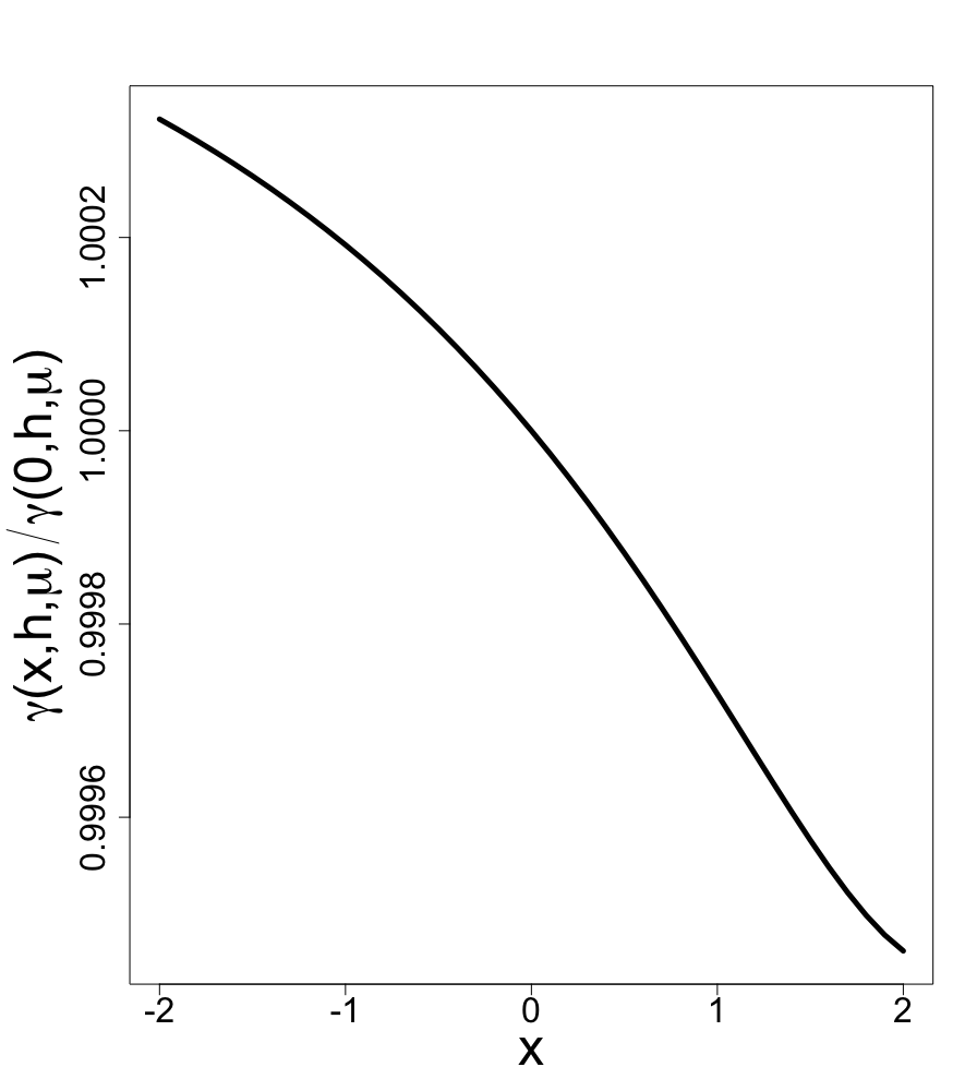
Figure 6: Ratio $\gamma(x,h,\mu)/\gamma(0,h,\mu)$ for $h=3$ and $\mu=3$.

In Table 1, we provide values of $\gamma(0,h,\mu)$ for different $\mu$, where the values of $h$ have been chosen to satisfy $\mathbb{E}_{0}(\tau(h))=C$ for $C=100,500,1000$; see (7.4) regarding computation of the ARL $\mathbb{E}_{0}(\tau(h))$.

As seen from Figures 3 and 4, the barrier $B_{1,1}(t;h,-\mu,\mu)$ is the main component of the barrier $B(t;h,0,-\mu,\mu)$. Instead of using the approximation ${\cal P}({h,\mu})\simeq\gamma(0,h,\mu)$ it is therefore tempting to use a simpler approximation ${\cal P}({h,\mu})\simeq\gamma_{1}(0,h,\mu)$, where

$$\gamma_{1}(x,h,\mu):={\rm P}\{S(t)\geq B(t;h,-\mu,\mu)\text{ for at least one }t\in[0,2]\,\big{|}S(0)=x\}=1-F_{h,-\mu,\mu}(1,1|\,x)$$

To compute values of $\gamma_{1}(0,h,\mu)$ we only need to evaluate a one-dimensional integral. Table 2 we show some values of $\gamma_{1}(0,h,\mu)$ for different $\mu$. Comparing the entries of Tables 1 and 2 we can observe that the quality of ${\cal P}({h,\mu})\simeq\gamma_{1}(0,h,\mu)$ is not too bad, especially for large $\mu$.

Approximation ${\cal P}({h,\mu})\simeq\gamma_{1}(0,h,\mu)$ can be improved if we average values of $\gamma_{1}(x,h,\mu)$ over an appropriate distribution for $x$. According to Section 2.4.2 in [10], one of possible appropriate distributions for $x$ has density

$$p(x)=\frac{\Phi(h)\varphi(x)-\Phi(x)\varphi(h)}{\Phi^{2}(h)-\varphi(h)\big{[}h\Phi(h)+\varphi(h)\big{]}}\,,\;\;x\leq h\,.$$

Define $\gamma_{2}(h,\mu)=\int_{-\infty}^{h}\gamma_{1}(x,h,\mu)p(x)dx$, which is a two-dimensional integral. As seen from comparison of Tables 1 and 3, the accuracy of the approximation ${\cal P}({h,\mu})\simeq\gamma_{2}(h,\mu)$ is almost the same as the accuracy of the main approximation ${\cal P}({h,\mu})\simeq\gamma(0,h,\mu)$. Computational cost of computing $\gamma_{2}(h,\mu)$ is similar to the cost for $\gamma(h,\mu)$.

To assess the impact the final line-segment in the barrier $B(t;h,0,-\mu,\mu)$ on power (the line-segment with gradient $\mu$ in Fig 6, $t\in[\nu,\nu+1]$), in Table 4 we document the values of $\gamma_{3}(0,h,\mu)$ for different $\mu$. Here

$$\gamma_{3}(x,h,\mu)\!\!\! := \!\!\!{\rm P}\{S(t)\geq B(t;h,0,-\mu)\text{ for at least one }t\in[1,2]\,\big{|}S(0)=x,\;\,S(t)<h,\forall{t\in[0,1]}\}$$

$$= \!\!\!1-\frac{{\rm P}\left\{S(t)<B(t;h,0,-\mu)\text{ for all }t\in[0,2]\,\big{|}S(0)=x\right\}}{{\rm P}\left\{S(t)<h\text{ for all }t\in[0,1]\big{|}S(0)=x\right\}}=1-\frac{F_{h,0,-\mu}(1,1|\,x)}{F_{h,0}(1|x)}$$

and $F_{h,0,-\mu}(1,1|\,0)$ can be computed using (4.6) with $b^{\prime}=\mu$. By comparing Tables 1 and 4, one can see the expected diminishing impact which the final line-segment in $B(t;h,0,-\mu,\mu)$ has on power, as $\mu$ increases. However, for small $\mu$ the contribution of this part of the barrier to power is significant suggesting it is not be sensible to approximate the power of our test with $\gamma_{3}(0,h,\mu)$.

$h=3.11$, $C\simeq 100$
$\mu$	$\gamma(0,3.11,\mu)$
2	0.3052
2.25	0.3876
2.5	0.4765
2.75	0.5676
3	0.6559
3.25	0.7371
3.5	0.8075
3.75	0.8653
4	0.9101
4.25	0.9429
4.5	0.9655
4.75	0.9802
5	0.9892

$h=3.63$, $C\simeq 500$
$\mu$	$\gamma(0,3.63,\mu)$
2	0.1384
2.25	0.1946
2.5	0.2638
2.75	0.3445
3	0.4338
3.25	0.5272
3.5	0.6197
3.75	0.7061
4	0.7824
4.25	0.8461
4.5	0.8961
4.75	0.9332
5	0.9592

$h=3.83$, $C\simeq 1000$
$\mu$	$\gamma(0,3.83,\mu)$
2	0.0956
2.25	0.1402
2.5	0.1979
2.75	0.2687
3	0.3510
3.25	0.4416
3.5	0.5358
3.75	0.6285
4	0.7146
4.25	0.7900
4.5	0.8525
4.75	0.9011
5	0.9370

Table 1: $\gamma(0,h,\mu)$ as a function of $\mu$ for three choices of ARL.

$h=3.11$, $C\simeq 100$
$\mu$	${\gamma_{1}}(0,3.11,\mu)$
2	0.2918
2.5	0.4645
3	0.6471
3.5	0.8021
4	0.9075
4.5	0.9644
5	0.9889

$h=3.63$, $C\simeq 500$
$\mu$	${\gamma_{1}}(0,3.63,\mu)$
2	0.1310
2.5	0.2553
3	0.4256
3.5	0.6132
4	0.7783
4.5	0.8940
5	0.9583

$h=3.83$, $C\simeq 1000$
$\mu$	${\gamma_{1}}(0,3.83,\mu)$
2	0.0903
2.5	0.1911
3	0.3438
3.5	0.5295
4	0.7101
4.5	0.8499
5	0.9358

Table 2: Values of $\gamma_{1}(0,h,\mu)$ for some $\mu$ and $h$.

$h=3.11$, $C\simeq 100$
$\mu$	${\gamma_{2}}(3.11,\mu)$
2	0.3047
2.5	0.4760
3	0.6555
3.5	0.8073
4	0.9100
4.5	0.9654
5	0.9892

$h=3.63$, $C\simeq 500$
$\mu$	${\gamma_{2}}(3.63,\mu)$
2	0.1383
2.5	0.2637
3	0.4337
3.5	0.6196
4	0.7824
4.5	0.8961
5	0.9592

$h=3.83$, $C\simeq 1000$
$\mu$	${\gamma_{2}}(3.83,\mu)$
2	0.0956
2.5	0.1978
3	0.3509
3.5	0.5358
4	0.7146
4.5	0.8524
5	0.9370

Table 3: Values of $\gamma_{2}(h,\mu)$ for some $\mu$ and $h$.

$h=3.11$, $C\simeq 100$
$\mu$	${\gamma_{3}}(0,3.11,\mu)$
2	0.2389
2.5	0.4017
3	0.5873
3.5	0.7567
4	0.8801
4.5	0.9514
5	0.9840

$h=3.63$, $C\simeq 500$
$\mu$	${\gamma_{3}}(0,3.63,\mu)$
2	0.1039
2.5	0.2131
3	0.3731
3.5	0.5611
4	0.7373
4.5	0.8685
5	0.9458

$h=3.83$, $C\simeq 1000$
$\mu$	${\gamma_{3}}(0,3.83,\mu)$
2	0.0708
2.5	0.1575
3	0.2974
3.5	0.4785
4	0.6657
4.5	0.8194
5	0.9192

Table 4: Values of $\gamma_{3}(0,h,\mu)$ for some $\mu$ and $h$.

7 Appendix A

7.1 First-passage probability $F_{a,b}(T\,|\,x)$ for $T\leq 1$

For $T\leq 1$, the first passage probability $F_{a,b}(T\,|\,x)$ has been well studied. An explicit formula was first derived in 1988 in [12, p.81] (published in Russian) and more than 20 years later it was independently derived in [13] and [14]. The authors of [12] and [14] also considered the case of piecewise-linear barriers.

In [12], the first passage probability $F_{a,b}(T\,|\,x)$ for $T\leq 1$ was obtained by using the fact $S(t)$ is a conditionally Markov process on the interval $[0,1]$. It was shown in [2] that after conditioning on $S(0)=x$, $S(t)$ can be expressed in terms of Brownian Motion as follows

$$S(t)=(2-t)W(g(t))+x(1-t),\,\,\,\,\,\,\,\,0\leq t\leq 1.$$

with $g(t)=t/(2-t)$. From this it follows that for $T\leq 1$

$$F_{a,b}(T\,|\,x)={\rm Pr}\bigg{(}W(g(t))<\frac{a+bt-x(1-t)}{2-t}\text{ for all }t\in[0,T]\bigg{)}.$$

Noting that $t={2g(t)}/({1+g(t)})$ and using the well known barrier crossing formula for the Brownian motion (see e.g. [15])

$$F_{a,b}(T\,|\,x)= \,{\rm Pr}\bigg{(}W(g(t))<\bigg{(}\frac{(a-x)(1+g(t))}{2}\bigg{)}+(x+b)g(t)\text{ for all }t\in[0,T]\bigg{)}$$

$$= \,{\rm Pr}\bigg{(}W(t^{\prime})<\bigg{(}\frac{a-x}{2}\bigg{)}+t^{\prime}\bigg{(}\frac{a+x}{2}+b\bigg{)}\text{ for all }t^{\prime}\in\bigg{[}0,\frac{T}{2-T}\bigg{]}\bigg{)}$$

$$= \,\Phi\bigg{(}\frac{b_{1}Z+a_{1}}{\sqrt{Z}}\bigg{)}-e^{-2a_{1}b_{1}}\Phi\bigg{(}\frac{b_{1}Z-a_{1}}{\sqrt{Z}}\bigg{)}\,\,,$$ (7.1)

where $Z={T}/({2-T})$, $b_{1}=({a+x})/{2}+b$ and $a_{1}=({a-x})/{2}$. This methodology, like many others, fails for $T>1$.

7.2 An approximation for $\mathbb{E}_{0}(\tau(h))$

Consider the unconditional probability (taken with respect to the standard normal distribution):

$$F_{h,0}(T):=\int_{-\infty}^{h}F_{h,0}(T\,|\,x)\varphi(x)dx\,.$$

Under $\mathbb{H}_{0}$, the distribution of $\tau(h)$ has the form:

$$(1-\Phi(h))\delta_{0}(ds)+q_{h}(s)ds\,,s\geq 0,$$

where $\delta_{0}(ds)$ is the delta-measure concentrated at 0 and

$$q_{h}(s)=-\frac{d}{ds}F_{h,0}(s),\;\;\;0<s<\infty\,$$

is the first-passage density. This yields

$$\mathbb{E}_{0}(\tau(h))=\int_{0}^{\infty}sq_{h}(s)ds.$$ (7.2)

There is no easy computationally convenient formula for $q_{h}(t)$ as expressions for $F_{h,0}(s)$ are very complex. For deriving approximations for $\mathbb{E}_{0}(\tau(h))$ we apply approximations for $F_{h,0}(s)$, discussed in [10]. One of the simplest (yet very accurate) approximation takes the following form:

$$F_{h,0}(T)\simeq F_{h,0}(2)\cdot\lambda(h)^{T-2},\;\;\mbox{for all $T>0$},$$ (7.3)

with $\lambda(h)=F_{h,0}(2)/F_{h,0}(1)$. Values of $F_{h,0}(2)$ must be numerically computed; approximations and simpler forms of $F_{h,0}(2)$ have been presented in [10] should one require an explicit formula. Using (7.3), we approximate the density $q_{h}(s)$ by

$$q_{h}(s)\simeq-F_{h,0}(2)\log[\lambda({h})]\cdot\lambda({h})^{s-2},\,\,\,0<s<\infty.$$

Evaluation of the integral in (7.2) yields

$$\mathbb{E}_{0}(\tau(h))\cong-\frac{F_{h,0}(2)}{\lambda({h})^{2}\log[\lambda({h})]}\,.$$ (7.4)

Numerical study shows that the approximation (7.4) is very accurate for all $h\geq 3$.

8 Appendix B

8.1 Proof of (4.1)

The proof of (4.1) follows similar steps to the proof of (2.5). The event $\Omega$ becomes

$$\Omega = \bigg{\{}W(t)<W(t+1)+a+bt<\ldots<W(t+T)+T(a+bt)+\frac{(T-1)T}{2}b$$

$$\,\,\,\,\,\,<W(t+T+1)+a(T+1)+bT+\frac{(T-1)T}{2}b+(b^{\prime}+Tb)t\,\,\,\,\,<\ldots<$$

$$\quad W(t+T+T^{\prime})+a(T+T^{\prime})+bTT^{\prime}+\frac{(T^{\prime}-1)T^{\prime}}{2}b^{\prime}+\frac{(T-1)T}{2}b+(T^{\prime}b^{\prime}+Tb)t$$

$$\quad\text{for all }t\in[0,1]\bigg{\}}.$$

As in the proof of (2.5), let $x_{i}=W(i)$, $i=0,\ldots,T+T^{\prime}+1$, where $W(1)=x_{1}=-x$. Then

$$F_{a,b,b^{\prime}}(T,T^{\prime}\,|\,x)\!=\!\int\!\!\!\!\!\! \cdots \!\!\!\!\!\!\int\!{\rm Pr}\{\Omega\,|\,W(0)\!=\!x_{0},\ldots,W(T+T^{\prime}+1)\!=\!x_{T+T^{\prime}+1},W(0)\!-\!W(1)\!=\!x\}$$ (8.1)

$$\!\!\!\!\times{\rm Pr}\{W(0)\!\in\!dx_{0},\ldots,W(T+T^{\prime}+1)\!\in\!dx_{T+T^{\prime}+1}\,\,|\,\,W(0)\!-\!W(1)\!=\!x\}.\;\;\;\;\;$$

Define the following processes which take different forms depending on the value of $i$:

$$W_{i}(t)\! = \!W(t+i)+i(a+bt)+\frac{(i-1)i}{2}b\,,\;\;\mbox{for $0\leq i\leq T$}\,;$$

$$W_{i}(t)\! = \!W(t+i)\!+\!ai\!+\!bT(i-T)\!+\!\frac{(i\!-\!T\!-\!1)(i\!-\!T)}{2}b^{\prime}\!+\!\frac{(T\!-\!1)T}{2}b\!+\!\{(i\!-\!T)b^{\prime}\!+\!Tb\}t,$$

for $T\!+\!1\leq i\leq T+T^{\prime}\!$, with $0\leq t\leq 1$ for all processes. The event $\Omega$ can now be expressed as

$$\qquad\Omega=\{W_{0}(t)<W_{1}(t)<\ldots<W_{T}(t)<\ldots<W_{T+T^{\prime}}(t)\text{ for all }t\in[0,1]\}.$$ (8.2)

Under the conditioning introduced in (8.1), depending on the size of $i$ we have: for $0\leq i\leq T$

$$W_{i}(0)=x_{i}+ia+\frac{(i-1)i}{2}b\,,\;\;\;W_{i}(1)=x_{i+1}+i(a+b)+\frac{(i-1)i}{2}b\,;$$

and for $T+1\leq i\leq T+T^{\prime}$

$$W_{i}(0) = x_{i}+ai+bT(i-T)\!+\!\frac{(i\!-\!T\!-\!1)(i\!-\!T)}{2}b^{\prime}\!+\!\frac{(T\!-\!1)T}{2}b\,,$$

$$W_{i}(1) = x_{i+1}+ai+bT(i-T)\!+\!\frac{(i\!-\!T\!-\!1)(i\!-\!T)}{2}b^{\prime}\!+\!\frac{(T\!-\!1)T}{2}b+\!(i\!-\!T)b^{\prime}\!+\!Tb\,.$$

Whence (8.1) can be expressed as

$$F_{a,b,b^{\prime}}(T,T^{\prime}\,|\,x)\!=\!\int\!\!\!\!\! \cdots \!\!\!\!\!\int{\rm Pr}\bigg{\{}\Omega\,\bigg{|}\,W_{i}(0)=x_{i}+ia+\frac{(i-1)i}{2}b\,,W_{i}(1)=x_{i+1}$$ (8.3)

$$\qquad+\,i(a+b)+\frac{(i-1)i}{2}b\,\,\,(0\leq i\leq T),W_{i}(0)=x_{i}\!+\!ai\!+\!bT(i\!-\!T)$$

$$\qquad+\,\frac{(i\!-\!T\!-\!1)(i\!-\!T)}{2}b^{\prime}\!+\!\frac{(T\!-\!1)T}{2}b\,,W_{i}(1)=x_{i+1}\!+\!ai\!+\!bT(i\!-\!T)\!$$

$$\qquad+\,\frac{(i\!-\!T\!-\!1)(i\!-\!T)}{2}b^{\prime}\!+\!\frac{(T\!-\!1)T}{2}b+\!(i\!-\!T)b^{\prime}\!+\!Tb\,\,\,$$

$$\qquad(T\leq i\leq T\!+\!T^{\prime}),\,W_{0}(0)\!-\!W_{0}(1)\!=\!x\bigg{\}}\times$$

$${\rm Pr}\{W(0)\!\in\!dx_{0},\ldots,W(T\!+\!T^{\prime}\!+\!1)\!\in\!dx_{T+T^{\prime}+1}\,|\,W(0)\!-\!W(1)\!=\!x\}.\;\;\;\;$$

The region of integration in (8.3) is determined from the following inequalities which, like in the proof of (4.1), ensure that the inequalities in (8.2) hold at $t=0$ and $t=1$:

$$x_{1}\!\!\! <\ldots< \!\!\!x_{T+1}\!+\!T(a+b)\!+\!\frac{(T\!-\!1)T}{2}b<x_{T+2}\!+\!a(T\!+\!1)\!+\!bT\!+\!\frac{(T\!-\!1)T}{2}b\!+\!b^{\prime}\!+\!Tb<\ldots<$$

$$\!\!\!x_{T+T^{\prime}+1}+a(T+T^{\prime})+bTT^{\prime}+\frac{(T^{\prime}\!-\!1)T^{\prime}}{2}b^{\prime}+\frac{(T\!-\!1)T}{2}b+\!T^{\prime}b^{\prime}\!+\!Tb.$$

From this, the upper limit of integration is infinity for all $x_{i}$. For $0\leq i\leq T+1$, the lower limit for $x_{i}$ is $x_{i-1}-a-(i-1)b$. For $T+2\leq i\leq T+T^{\prime}+1$, the lower limit for $x_{i}$ is $x_{i-1}-a-bT-b^{\prime}(i-T-1)$.

Application of (2.1) with $n=T+T^{\prime}$ provides

$${\rm Pr}\bigg{\{}\!\!\!\!\!\! \Omega \!\!\!\!\!\!\,\bigg{|}\,W_{i}(0)=x_{i}+ia+\frac{(i-1)i}{2}b\,,W_{i}(1)=x_{i+1}+i(a+b)+\frac{(i-1)i}{2}b\,\,(0\leq i\leq T)$$

$$\!\!W_{i}(0)=x_{i}+ai+bT(i-T)\!+\!\frac{(i\!-\!T\!-\!1)(i\!-\!T)}{2}b^{\prime}\!+\!\frac{(T\!-\!1)T}{2}b\,,$$

$$\!\!W_{i}(1)=x_{i+1}+ai+bT(i-T)\!+\!\frac{(i\!-\!T\!-\!1)(i\!-\!T)}{2}b^{\prime}\!+\!\frac{(T\!-\!1)T}{2}b+\!(i\!-\!T)b^{\prime}\!+\!Tb\,$$

$$\!\!(T\leq i\leq T+T^{\prime}),W_{0}(0)\!-\!W_{0}(1)\!=\!x\bigg{\}}$$

$$= \exp(-|{\boldsymbol{\mu}}_{3}|^{2}/2+{\boldsymbol{\mu}}_{3}\cdot(\textbf{c}_{3}-\textbf{a}_{3}))\det[\varphi({{a}_{3}}_{i},{{c}_{3}}_{j})]_{i,j=0}^{T^{\prime}+T}/\prod_{i=0}^{T+T^{\prime}}\varphi({{a}_{3}}_{i}-{{c}_{3}}_{i}+{{\mu}_{3}}_{i}),$$

where $\boldsymbol{\mu}_{3}$ and $\textbf{a}_{3}$ are given in (4.2) and $\textbf{c}_{3}$ is given in (4.3). The second probability in the right hand side of (8.3) is $\prod_{i=1}^{T+T^{\prime}}\varphi(x_{i}-x_{i+1})$. We complete the proof by collating all terms and noting

$$\prod_{i=0}^{T+T^{\prime}}\varphi({{a}_{3}}_{i}-{{c}_{3}}_{i}+{{\mu}_{3}}_{i})=\prod_{i=0}^{T+T^{\prime}}\varphi(x_{i}-x_{i+1})\,.$$

$\Box$

8.2 Proof of (5.3)

Like the proof of (4.1), the proof of (5.3) is similar to the proof of (2.5). We modify the event $\Omega$ as follows:

$$\Omega = \bigg{\{}W(t)<W(t+1)+a+bt<W(t+2)+2a+b+bt+b^{\prime}t<$$

$$\quad W(t+3)+3a+2b+b^{\prime}+(b+b^{\prime}+b^{\prime\prime})t\text{ for all }t\in[0,1]\bigg{\}}.$$

By the law of total probability,

$$F_{a,b,b^{\prime},b^{\prime\prime}}(3\,|\,x)\!=\!\int\!\!\!\!\! \cdots \!\!\!\!\!\int{\rm Pr}\{\Omega\,|\,W(0)\!=\!x_{0},\ldots,W(4)\!=\!x_{4},W(0)\!-\!W(1)\!=\!x\}$$ (8.4)

$$\!\!\!\times\,{\rm Pr}\{W(0)\!\in\!dx_{0},\ldots,W(4)\!\in\!dx_{4}\,\,|\,\,W(0)\!-\!W(1)\!=\!x\}.$$

Define individually the following processes:

$$W_{0}(t) = W(t)$$

$$W_{1}(t) = a+bt+W(t+1)$$

$$W_{2}(t) = 2a+b+(b+b^{\prime})t+W(t+2)$$

$$W_{3}(t) = 3a+2b+b^{\prime}+(b+b^{\prime}+b^{\prime\prime})t+W(t+3)$$

with $0\leq t\leq 1$ for all processes. The event $\Omega$ can be re-written as

$$\Omega=\{W_{0}(t)<W_{1}(t)<W_{2}(t)<W_{3}(t)\text{ for all }t\in[0,1]\}.$$ (8.5)

The conditioning introduced in (8.4) results in:

$$W_{0}(0) = 0$$

$$W_{1}(0) = a+x_{1}$$

$$W_{2}(0) = 2a+b+x_{2}$$

$$W_{3}(0) = 3a+2b+b^{\prime}+x_{3}$$

$$W_{0}(1) = x_{1}$$

$$W_{1}(1) = a+b+x_{2}$$

$$W_{2}(1) = 2a+2b+b^{\prime}+x_{3}$$

$$W_{3}(1) = 3a+3b+2b^{\prime}+b^{\prime\prime}+x_{4}.$$

From this, we can express (8.4) as:

$$F_{a,b,b^{\prime},b^{\prime\prime}}(3\,|\,x)\!\!=\!\!\int\!\!\!\!\! \cdots \!\!\!\!\!\int{\rm Pr}\bigg{\{}\Omega\,\bigg{|}\,W_{0}(0)=0,\ldots,W_{3}(0)\!=\!3a\!+\!2b\!+\!b^{\prime}\!+\!x_{3},W_{0}(1)=x_{1},\ldots,$$ (8.6)

$$\qquad W_{3}(1)=3a+3b+2b^{\prime}+b^{\prime\prime}+x_{4},W_{0}(0)\!-\!W_{0}(1)\!=\!x\bigg{\}}$$

$$\,\,\,\,\times{\rm Pr}\{W(0)\!\in\!dx_{0},\ldots,W(4)\!\in\!dx_{4}\,\,|\,\,W(0)\!-\!W(1)\!=\!x\}.$$

The region of integration for (8.6) is determined from the following inequalities (see proof of (2.5) for similar discussion):

$$x_{1}<x_{2}+a+b<x_{3}+2a+2b+b^{\prime}<x_{4}+3a+3b+2b^{\prime}+b^{\prime\prime}.$$

Thus, the upper limit of integration is infinity for all $x_{i}$. For integration with respect to $x_{4}$, the lower limit is $x_{3}-a-b-b^{\prime}-b^{\prime\prime}$. For integration with respect $x_{3}$, the lower limit is $x_{2}-a-b-b^{\prime}$. Finally, for $x_{2}$, the lower limit is $x_{1}-a-b=-x-a-b$. Now using (2.1) with $n=3$ we obtain

$${\rm Pr}\bigg{\{}\Omega\!\!\!\!\! | \!\!\!\!\!W_{0}(0)=0,\ldots,W_{3}(0)=3a+2b+b^{\prime}+x_{3}$$

$$\!\!\!\!\!W_{0}(1)=x_{1},\ldots,W_{3}(1)=3a+3b+2b^{\prime}+b^{\prime\prime}+x_{4},W_{0}(0)\!-\!W_{0}(1)\!=\!x\bigg{\}}$$

$$= \exp(-|{\boldsymbol{\mu}}_{4}|^{2}/2+{\boldsymbol{\mu}}_{4}\cdot(\textbf{c}_{4}-\textbf{a}_{4}))\det[\varphi({{a}_{4}}_{i},{{c}_{4}}_{j})]_{i,j=0}^{3}/\prod_{i=0}^{3}\varphi({{a}_{4}}_{i}-{{c}_{4}}_{i}+{{\mu}_{4}}_{i}),$$

$\boldsymbol{\mu}_{4}$, $\textbf{a}_{4}$ and $\textbf{c}_{4}$ are given in (5.2). The second probability in the right hand side of (8.6) is $\prod_{i=1}^{3}\varphi(x_{i}-x_{i+1})$. Using the fact

$$\prod_{i=0}^{3}\varphi({{a}_{4}}_{i}-{{c}_{4}}_{i}+{{\mu}_{4}}_{i})=\prod_{i=0}^{3}\varphi(x_{i}-x_{i+1}),$$

and collecting all results we complete the proof. $\Box$

References

• [1] D. Slepian. First passage time for a particular Gaussian process. The Annals of Mathematical Statistics, 32(2):610–612, 1961.
• [2] C.B. Mehr and J.A. McFadden. Certain properties of Gaussian processes and their first-passage times. Journal of the Royal Statistical Society. Series B (Methodological), 27(3):505–522, 1965.
• [3] L. Shepp. First passage time for a particular Gaussian process. The Annals of Mathematical Statistics, 42(3):946–951, 1971.
• [4] S. Karlin and J. McGregor. Coincidence probabilities. Pacific Journal of Mathematics, 9(4):1141–1164, 1959.
• [5] M. Katori. Reciprocal time relation of noncolliding Brownian motion with drift. Journal of Statistical Physics, 148(1):38–52, 2012.
• [6] M. Pollak and D. Siegmund. A diffusion process and its applications to detecting a change in the drift of Brownian motion. Biometrika, 72(2):267–280, 1985.
• [7] G. Moustakides. Optimality of the CUSUM procedure in continuous time. The Annals of Statistics, 32(1):302–315, 2004.
• [8] A. Polunchenko. Asymptotic near-minimaxity of the randomized Shiryaev–Roberts–Pollak change-point detection procedure in continuous time. Theory of Probability & Its Applications, 62(4):617–631, 2018.
• [9] A. Polunchenko and A. Tartakovsky. On optimality of the Shiryaev–Roberts procedure for detecting a change in distribution. The Annals of Statistics, 38(6):3445–3457, 2010.
• [10] J. Noonan and A. Zhigljavsky. Approximating Shepp’s constants for the Slepian process. arXiv preprint arXiv:1812.11101, 2018.
• [11] U. Grenander. Abstract inference. John Wiley & Sons, 1981.
• [12] A. Zhigljavsky and A. Kraskovsky. Detection of abrupt changes of random processes in radiotechnics problems. St. Petersburg University Press, 1988. (in Russian).
• [13] W. Bischoff and A. Gegg. Boundary crossing probabilities for (q, d)-Slepian-processes. Statistics & Probability Letters, 118:139–144, 2016.
• [14] P. Deng. Boundary non-crossing probabilities for Slepian process. Statistics & Probability Letters, 122:28–35, 2017.
• [15] D. Siegmund. Boundary crossing probabilities and statistical applications. The Annals of Statistics, 14(2):361–404, 1986.