XXXX-XXXX

Large-amplitude quadrupole shape mixing probed by the $(p,p^{\prime})$ reaction : a model analysis

Abstract

To discuss a possible observation of large-amplitude nuclear shape mixing by nuclear reaction, we employ a simple collective model and evaluate transition densities, with which the differential cross sections are obtained through the microscopic coupled-channel calculation. Assuming the spherical-to-prolate shape transition, we focus on large-amplitude shape mixing associated with the softness of the collective potential in the $\beta$ direction. We introduce a simple model based on the five-dimensional quadrupole collective Hamiltonian, which simulates a chain of isotopes that exhibit spherical-to-prolate shape phase transition. Taking ¹⁵⁴Sm as an example and controlling the model parameters, we study how the large-amplitude shape mixing affects the elastic and inelastic proton scatterings. The calculated results suggest that the inelastic cross section of the $2_{2}^{+}$ state tells us an important role of the quadrupole shape mixing.

xxxx, xxx

In low-lying states in atomic nuclei quadrupole deformation plays an important role. The collectivity associated with the nuclear quadrupole deformation is experimentally studied through excitation energies, $B(E2)$, spectroscopic quadrupole moments and so on. Theoretically, one of the standard tools to describe the quadrupole deformation and rotation dynamics is the five-dimensional (5D) quadrupole collective Hamiltonian Bohr1975 ; Belyaev1965 ; Kumar1967 ; Prochniak2009 ; Matsuyanagi2016 , and it is widely used in nuclear structure studies. The dynamical variables in this 5D collective Hamiltonian approach are the magnitude and triaxiality of quadrupole deformation $(\beta,\gamma)$, and the three Euler angles. The collective Hamiltonian is characterized by the collective potential and inertial masses, which are introduced either phenomenologically or microscopically. By solving the collective Schrödinger equation, one can describe large-amplitude quadrupole shape mixing dynamics as well as three-dimensional nuclear rotation.

There exist some preceding studies on nuclear shape mixing dynamics by means of electron and nucleon scatterings. The electron scattering is a powerful tool to determine the charge distribution and transition charge densities. In Ref. Phan1988 ; Boeglin1988 ; Sandor1991 , the collective Hamiltonian microscopically derived was used to evaluate the transition densities including dynamical deformation. It is also worth mentioning here that, recently, Yao et al. proposed a method of calculating form factors and transition densities within the beyond-mean-field framework of particle-number and angular-momentum projected generator coordinate method Yao2015 . In the analysis of the nucleon scattering experiments in the 1980s Mirzaa1985 ; Delaroche1987 ; Clegg1989 ; Hicks1989 , several nuclear structure models were adopted in conjunction with the coupled-channel calculation to investigate the $\gamma$-softness in the low-lying excited states in the Pt-Os region, and it was found that some isotopes are best described by $\gamma$-soft models.

In this Letter, we discuss such a possible observation of large-amplitude shape mixing by nuclear reaction. We investigate the effect of quadrupole shape mixing on the proton elastic and inelastic scatterings with use of a simple collective model based on the 5D quadrupole collective Hamiltonian. Here, we focus on shape mixing dynamics in the spherical-to-prolate transition, assuming transitional nuclei in the $A\sim 150$ mass region, and apply our model to a samarium isotope. The purpose of this study is, however, to grasp the gross feature of the effects of the quadrupole deformation and large-amplitude shape mixing dynamics on the observable differential cross sections for the $(p,p^{\prime})$ reaction from a general point of view.

In Ref. Sato2010 , the triaxial deformation dynamics was studied by introducing the collective potential and inertial masses in the collective Hamiltonian phenomenologically. We follow this approach and extend the model proposed in Ref. Sato2010 to study the case where the collective potential is soft against the $\beta$ deformation. The 5D collective Hamiltonian is written as

$$\mathcal{H}_{\rm coll} =T_{\rm vib}+T_{\rm rot}+V_{\rm coll}(\beta,\gamma),$$ (1)

$$T_{\rm vib} =\frac{1}{2}D_{\beta\beta}\dot{\beta}^{2}+D_{\beta\gamma}\dot{\beta}\dot{\gamma}+\frac{1}{2}D_{\gamma\gamma}\dot{\gamma}^{2},$$ (2)

$$T_{\rm rot} =\frac{1}{2}\sum_{k=1}^{3}\mathcal{J}_{k}(\beta,\gamma)\omega_{k}^{2},$$ (3)

where $T_{\rm vib}$ and $T_{\rm rot}$ are the vibrational and rotational kinetic energies, respectively, and $V_{\rm coll}$ is the collective potential. The 5D collective Hamiltonian is characterized by seven quantities: the collective potential $V_{\rm coll}(\beta,\gamma)$, three vibrational masses $D_{\beta\beta}(\beta,\gamma),D_{\beta\gamma}(\beta,\gamma),D_{\gamma\gamma}(\beta,\gamma)$, and three moments of inertia $\mathcal{J}_{k}(\beta,\gamma)~{}(k=1,2,3)$. The collective potential $V_{\rm coll}(\beta,\gamma)$ must be a scalar under rotation, so it can be written as a function of $\beta^{2}$ and $\beta^{3}\cos 3\gamma$ Bohr1975 . We consider three typical situations: a spherical vibrator, a prolate rotor, and a transitional nucleus between the former two limits. To simulate those typical situations, we adopt the collective potential in the following form:

$$V_{\rm coll}(\beta,\gamma)= \frac{1}{2}C_{2}\beta^{2}+\frac{1}{2}C_{4}\left(\beta^{2}-\beta^{2}_{0}\right)^{2}+C_{6}\beta^{6}+v_{1}\beta^{3}\cos 3\gamma,$$ (4)

which is a modification of the potential in Ref. Sato2010 . The inertial mass parameters are the same as used in Ref. Sato2010 :

$$D_{\beta\beta}(\beta,\gamma) =D\left(1-\epsilon^{\prime}\beta\cos 3\gamma\right),$$ (5)

$$D_{\gamma\gamma}(\beta,\gamma) =D\beta^{2}\left(1+\epsilon^{\prime}\beta\cos 3\gamma\right),$$ (6)

$$D_{\beta\gamma}(\beta,\gamma) =D\epsilon^{\prime}\beta\sin 3\gamma,$$ (7)

$$D_{k}(\beta,\gamma) =D\left(1+\epsilon^{\prime}\beta\cos\gamma_{k}\right)\,\,(k=1,2,3),$$ (8)

where $\gamma_{k}=\gamma-(2\pi k)/3$, and the three moments of inertia are given by $\mathcal{J}_{k}(\beta,\gamma)=4\beta^{2}D_{k}(\beta,\gamma)\sin^{2}\gamma_{k}$. By controlling the parameters in Eqs. (4)–(8), we simulate the three typical situations mentioned above. After quantizing the collective Hamiltonian Eq. (1), we solve the collective Schrödinger equation and obtain the collective wave functions

$$\Psi_{\alpha IM}(\beta,\gamma,\Omega)=\sum_{K:{\rm even}}\Phi_{\alpha IK}(\beta,\gamma)\langle\Omega|IMK\rangle.$$ (9)

The parameter sets in the collective potential and inertial masses to simulate the three situations are listed in Table 1. In all the calculations, we set $D=50$ MeV^-1. The spherical case is treated as the 5D harmonic oscillator (HO). We plot in Fig. 1 the collective potentials $V_{\rm coll}(\beta,\gamma)$ obtained with these three parameter sets. While in the prolate case there is an absolute minimum around $\beta=0.35$, the collective potential is soft along the $\beta$ direction in the transitional case. The parameter $\epsilon^{\prime}$ in Eqs. (5)–(8) controls the oblate-prolate asymmetry. When $\epsilon^{\prime}$ is positive (negative), oblate (prolate) shape is favored to reduce the rotational energy. For these three parameter sets, we solve the collective Schrödinger equation and obtain the excitation energies and collective wave functions. Note that these parameters are not adjusted by fitting to specific experimental data but determined to simulate typical situations widely observed in the nuclear chart. By scaling the parameters $C_{i}~{}(i=2,4,6),v_{1},$ and $D^{-1}$ simultaneously, one can scale the excitation energies with the collective wave functions unchanged. Therefore, only the ratios of the excitation energies between excited states such as $R_{4/2}=E(4_{1}^{+})/E(2_{1}^{+})$ are meaningful. The obtained $R_{4/2}$ values are 2.0, 2.2, and 3.0 for the spherical, transitional and prolate parameter sets, respectively. Note that although this “prolate” parameter set simulates a prolately deformed rotor, it is not an ideal rigid rotor but contains shape fluctuation. We have confirmed that the deviation between the ideal rigid rotor and prolately deformed rotor is very small on the proton elastic and inelastic scatterings.

	Choice of parameters
spherical (5DHO)	$C_{2}=50$
prolately deformed	$C_{4}=800,\beta_{0}^{2}=0.1,v_{1}=-150,C_{6}=1000,\epsilon=-0.5$
spherical-prolate transitional	$C_{4}=800,v_{1}=-200,C_{6}=1000$

Table 1: The parameter sets to simulate the three typical situations. We take $D=50$ MeV^-1 for all the three calculations. The parameters in Eqs. (4)–(8) which are not shown above are zero. Here, $\epsilon$ is defined by $\epsilon^{\prime}=\epsilon/\beta_{0}$. All the parameters other than the two dimensionless ones, $\beta_{0}$ and $\epsilon$, are in units of MeV.

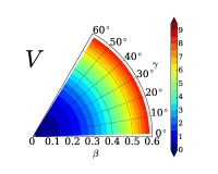
(a) spherical vibrator

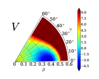
(b) prolately-deformed

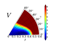
(c) spherical-prolate transitional

Figure 1: Collective potential $V_{\rm coll}(\beta,\gamma)$ [MeV] defined by Eq. (4) with the parameter sets in Table 1.

For the eigenstates $\Psi_{\alpha IM}(\beta,\gamma,\Omega)$ obtained with the collective Hamiltonian for each parameter set, we calculate the transition density matrix elements,

$$\langle\alpha^{\prime}I^{\prime}M^{\prime}|\hat{\rho}_{n(p)}({\bm{r}})|\alpha IM\rangle=\sum_{\mu\nu}(IM\mu\nu|I\mu I^{\prime}M^{\prime})\rho_{n(p),\alpha^{\prime}I^{\prime}\alpha I}^{\mu}(r)Y_{\mu\nu}^{*}(\theta,\varphi),$$ (10)

where the neutron (proton) transition density operator is given by $\hat{\rho}_{n(p)}({\bm{r}})=\sum_{i=1}^{N(Z)}\delta({\bm{r}-\bm{r}_{i}})$, and we have used the Wigner–Eckart theorem Edmonds1996 .

To evaluate the above matrix elements, the proton and neutron densities are needed for intrinsic states $\Phi_{\alpha IK}(\beta,\gamma)$. As we are taking a phenomenological approach, we solve the deformed Woods–Saxon (WS) potential problem with the $\beta$-$\gamma$ constraint on the mesh point $(\beta_{i},\gamma_{j})$ instead of performing microscopic calculation such as constrained Hartree–Fock–Bogoliubov calculation. Here we employ the following mesh points on the $\beta$-$\gamma$ plane: $\beta_{i}=(i-1/2)\Delta\beta,\gamma_{i}=(i-1/2)\Delta\gamma~{}(i=1,\cdots,20)$ with $\Delta\beta=0.03$ and $\Delta\gamma=3.0^{\circ}$. For this calculation, we used TRIAXIAL2014 Mohammed-Azizi2014 , which solves one-body problem with the deformed WS, the spin-orbit, and the Coulomb potentials. For the parameters of the deformed WS potential, the universal parameter set in Ref. Kahane1989 was adopted.

With the transition density, we obtain the proton elastic and inelastic cross sections based on the microscopic coupled-channel (MCC) calculation. Namely, the diagonal and transition potentials used in the coupled-channel (CC) calculation are derived from the folding procedure. In this Letter, we apply the JLM complex nucleon-nucleon interaction JLM1977 to the MCC calculation in the same as in Ref. takashina2008 . The JLM interaction is usually written in the form of

$$v_{NN}(s;\rho,E)=\frac{V(\rho,E)}{(t\sqrt{\pi})^{3}}\exp{\left(-\frac{s^{2}}{t^{2}}\right)}+i\frac{W(\rho,E)}{(t\sqrt{\pi})^{3}}\exp{\left(-\frac{s^{2}}{t^{2}}\right)},$$ (11)

where $V(\rho,E)$ and $W(\rho,E)$ are the strength of the real and imaginary parts, respectively. They include the isoscalar and isovector components. $\rho$ and $E$ are the nucleon density and the incident proton energy, respectively. $t$ is the range parameter of the nucleon-nucleon interaction. We fix the $t$ value to be 1.2 according to Ref. JLM1977 . The renormalization factor, which is often used to adjust the strength of the potential based on the folding model, is not applied in this Letter.

We apply our model introduced above to the proton elastic and inelastic scatterings by ¹⁵⁴Sm. It is well known that a spherical-to-prolate shape transition occurs with increasing the neutron number in samarium isotopes in this mass region. Actually, the experimental value of $R_{4/2}$ for ¹⁵⁴Sm is 3.2 and the experimental $\beta_{2}$ is 0.34 NNDC , which implies that the shape phase transition to the deformed shape already occurred. Although ¹⁵⁰Sm exhibits more transitional character ($R_{4/2}^{\rm exp.}=2.3$), we will show the results of ¹⁵⁴Sm for the following reasons. First, the abundance of ¹⁵⁴Sm is enough and the experimental data is also plenty. Second, in this phenomenological analysis the difference in the neutron number by four only plays a minor role.

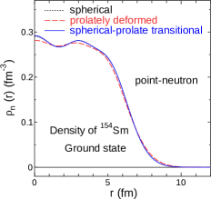
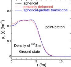
Figure 2: The point-neutron and point-proton density distributions obtained with the spherical (dotted line), prolate (dashed), and transitional (solid) models.

Figure 2 shows the point-neutron and point-proton densities distributions for the ground state obtained with the spherical, prolate, and transitional models. The neutron and proton density distributions in the transitional model almost coincide with those in the spherical HO model. We can see a difference between the density distribution derived from the prolately deformed model and those derived from the spherical HO and transitional models, especially for the tail part. In the prolate case, the tail part of the nuclear density in the laboratory frame is expanded by the deformation. The reason why the spherical and transitional models give similar density distributions can be attributed to their ground-state collective wave functions. The ground-state collective wave function in the transitional model [shown in Fig. 6(a)] spreads around the sphericity and is similar to that in the spherical HO model (not shown here), which leads to almost the same density distribution in the ground state. In Ref. minomo2011 , the deformation effect is discussed on the total reaction cross section. Below, the effect of the difference in the density distributions will be briefly discussed on the proton elastic cross section.

We show in Fig. 3 the calculated elastic and inelastic scattering cross sections at $E_{p}=35$, 65, and 66.5 MeV in comparison with the experimental data. For the elastic scattering, the calculated cross sections reasonably reproduce the experimental data. In detail, the calculated results for the prolate model deviate from those for the spherical and transitional models for backward angle, which is caused by the difference in the tail part of the density distribution of the ground state as mentioned above.

Note that, in this calculation, we have not adjusted any parameters in our model (those in the deformed WS model, the model collective Hamiltonians, and the JLM interaction), other than a rough adjustment of $\beta_{0}=0.33$ for the prolate rotor model. We have seen that the backward elastic scattering may be sensitive to the tail part of the ground-state density distribution. It can be affected not only by deformation but also by the diffuseness of the nuclear surface in the intrinsic frame. We have not adjusted the diffuseness parameters in the deformed WS potential as mentioned above.

For the inelastic scattering, the calculated cross sections also reproduce the experimental data. There is little difference between the results obtained with the spherical HO and the transitional models not only for the elastic differential cross sections but also for the inelastic differential cross sections for the yrast $2^{+},4^{+},$ and $6^{+}$ states.

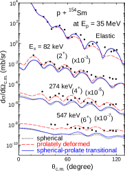
(a) $E_{p}=35$MeV

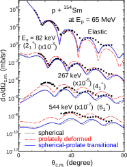
(b) $E_{p}=65$MeV

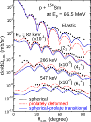
(c) $E_{p}=66.5$MeV

Figure 3: The calculated elastic and inelastic differential cross sections of the $p$ + ¹⁵⁴Sm system in comparison with experimental data exp-0350 ; exp-0650 ; exp-0665 at $E_{p}=$35, 65, and 66.5 MeV. The differential cross sections for the spherical, prolate, and transitional collective Hamiltonians are indicated by dotted, dashed, and solid lines, respectively.

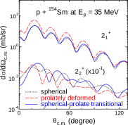
(a) $E_{p}=35$MeV

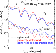
(b) $E_{p}=65$MeV

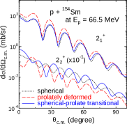
(c) $E_{p}=66.5$MeV

Figure 4: Same as Fig. 3 but for the inelastic differential cross section for the $2^{+}_{1}$ and $2_{2}^{+}$ states.

We apply our models to the non-yrast states to investigate the effect of the quadrupole shape mixing. In Fig. 4, the inelastic differential cross sections at $E_{p}=$ 35, 65, and 66.5 MeV for the $2_{2}^{+}$ state are displayed. Here, we plot the inelastic differential cross sections for the $2_{1}^{+}$ state again for comparison of the diffraction pattern. For the $2_{1}^{+}$ state, the three models give similar angular distributions. On the other hand, the calculated diffraction patterns are completely different for the $2_{2}^{+}$ state. Especially, whereas the positions of the peaks for the spherical and prolate models are almost the same, we clearly observe that the positions of peaks for the transitional model are shifted to backward compared with those of the other two models. This shift turns out to remain even if we disregard the multistep processes. Thus, it will be due to the difference in the calculated transition densities.

We plot in Fig. 5 the transition densities multiplied by $r^{2}$, $r^{2}\rho^{2}_{n(p)}(r)$, for the $0_{1}^{+}\rightarrow 2_{1}^{+}$ and $0_{1}^{+}\rightarrow 2_{2}^{+}$ transitions. For the $0_{1}^{+}\rightarrow 2_{1}^{+}$ transition, although the peak height for the prolate shape is larger than the other two, the structures of the transition densities obtained with the three calculations are similar to one another. On the other hand, the transition densities for the $0_{1}^{+}\rightarrow 2_{2}^{+}$ transition exhibit a rather different behavior. Because the neutron and proton transition densities have similar structure, we shall focus on the neutron transition density below. We see that, in the spherical and prolate cases, the main peak of the transition density is located around $r=8$ fm. In the transitional case, the main peak is located in an inner region around $r=6$ fm.

One may understand the difference between the prolate and transitional cases in a relatively simple way as follows, while a more detailed analysis is required for the spherical case. We show in Fig. 6 the collective wave functions squared $\sum_{K}|\Phi_{\alpha IK}(\beta,\gamma)|^{2}$ calculated for the $0_{1}^{+},2_{1}^{+}$, and $2_{2}^{+}$ states. While, in the prolate case, the collective wave function squared in the ground band are localized around the prolate potential minimum, that for the $2_{2}^{+}$ state has a two-peak structure on the prolate side. In this case, the $K=0$ component of the collective wave functions dominates over the $K\neq 0$ components, and the $Y_{20}$ component of the intrinsic density gives a main contribution to the transition density from $0_{1}^{+}$ to $2^{+}$ states. We also plot in Fig. 7 the $Y_{20}$ component of the neutron density $\rho^{20}(r;\beta,\gamma)$ for the intrinsic state with $(\beta,\gamma=1.5^{\circ})$. One can see that the peak of $\rho^{20}_{n}(r;\beta,\gamma)$ develops with increasing $\beta$. The $2_{2}^{+}$ state is a $\beta$-vibrational state, and the collective wave function $\Phi_{2_{2}^{+},K=0}(\beta,\gamma)$ has a node around $\beta=0.3$. The first peak around $\beta=0.2$ and the second peak around $\beta=0.4$ give a positive and negative contributions to the transition density, respectively. The contribution from the second peak dominates over the first, which leads to the transition density shown in Fig. 5(b).

In the transitional case, we can see that, there is strong $\beta$-$\gamma$ coupling, and the collective wave function of the $2_{2}^{+}$ state exhibits the $\gamma$-vibrational character as well as the $\beta$-vibrational one. There is a prolate peak around $\beta=0.3$ as in the prolate case, although the peak height is smaller. This peak contributes to a dip of the transition density in an outer region. The other component of the collective wave function squared spreading over the triaxial-oblate region gives a dominant contribution to the transition density shown in Fig. 5(b). Thus, the strong shape mixing in transitional nuclei may affect the inelastic differential cross sections.

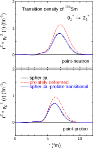
(a) $0_{1}^{+}\rightarrow 2_{1}^{+}$

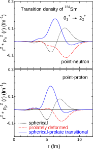
(b) $0_{1}^{+}\rightarrow 2_{2}^{+}$

Figure 5: The neutron (proton) transition densities multiplied by $r^{2}$, $r^{2}\rho^{2}_{n(p)}(r)$, from the ground state to the first and second $2^{+}$ states in ¹⁵⁴Sm. The calculated results for the spherical, prolate, and transitional parameter sets are indicated by dotted, dashed, and solid lines, respectively.

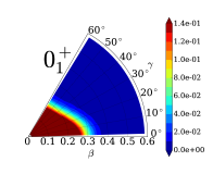
(a) transitional $0_{1}^{+}$

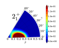
(b) transitional $2_{1}^{+}$

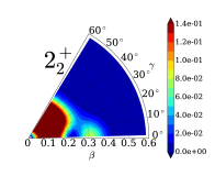
(c) transitional $2_{2}^{+}$

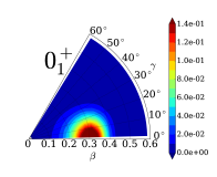
(d) prolate $0_{1}^{+}$

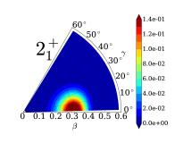
(e) prolate $2_{1}^{+}$

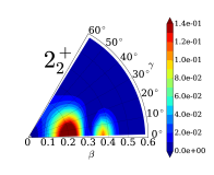
(f) prolate $2_{2}^{+}$

Figure 6: The collective wave function squared $\sum_{K}|\Phi_{\alpha IK}(\beta,\gamma)|^{2}$ calculated for the $0_{1}^{+},2_{1}^{+}$, and $2_{2}^{+}$ states.

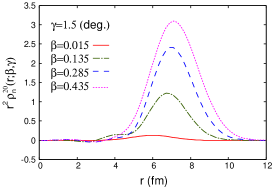
Figure 7: The $Y_{20}$ component of the neutron density multiplied by $r^{2}$, $r^{2}\rho^{20}_{\rm n}(r;\beta,\gamma)$, for the intrinsic states with $(\beta,\gamma=1.5^{\circ})$.

In this study, to discuss a possible observation of large-amplitude shape mixing in transitional nuclei by nuclear reaction, we adopted a phenomenological model based on the 5D quadrupole collective Hamiltonian simulating isotopes exhibiting the spherical-to-prolate shape transition, and investigated the effect of the large-amplitude quadrupole shape mixing on the proton elastic and inelastic differential cross sections. We have seen that, as a result of the strong $\beta$-$\gamma$ coupling in transitional nuclei, the transition density for the $2_{2}^{+}$ state exhibits structure different from those for the spherical vibrator and the prolate rotor, which leads to the shift of the diffraction pattern of the inelastic differential cross section for the $2_{2}^{+}$ state. Thus, it can be a experimental signature of the strong $\beta$-$\gamma$ coupling and large-amplitude quadrupole shape mixing in spherical-to-prolate transitional nuclei.

In this Letter, we have used a simple model to calculate the transition densities. The model we have used is a modification of the model in Ref. Sato2010 , and we omitted the $\beta^{6}\cos^{2}3\gamma$ term here. By adding this term to the collective potential, our model can accommodate the oblate-prolate shape coexistence, triaxial rotor, and $\gamma$-soft limits, which enables us to perform a similar analysis on the large-amplitude triaxial deformation dynamics. Moreover, it would be interesting to use the transition densities calculated microscopically and check the validity of our simple model. One of the authors (KS) and his collaborators have developed a method for microscopically determining the 5D quadrupole collective Hamiltonian, the constrained Hartree–Fock–Bogoliubov plus local quasiparticle random phase approximation (CHFB+LQRPA) method. One of the advantages of this method is that one can take into account the contribution from the time-odd mean field to the inertial mass unlike the widely-used cranking formula, and it was successfully applied to a variety of the large-amplitude quadrupole collective dynamics Hinohara2010b ; Sato2011 ; Watanabe2011 ; Hinohara2011a ; Yoshida2011 ; Hinohara2011b ; Hinohara2012 ; Sato2012 . Microscopic calculation of the transition density with the CHFB+LQRPA method will be reported in a future publication. In addition, the CHFB+LQRPA method is an approximate version of the adiabatic self-consistent collective-coordinate (ASCC) theory with two-dimensional collective coordinate Matsuo2000 ; Hinohara2007 . The ASCC theory is an advanced version of the adiabatic time-dependent Hartree–Fock–Bogoliubov theory, and has been successfully used to nuclear structure and reaction studies Hinohara2008 ; Hinohara2009 ; Wen2016 ; Wen2017 . In recent studies Sato2015 ; Sato2017a ; Sato2017b ; Sato2018 , theoretical aspect of the ASCC theory has been highly elucidated, and an extension of the theory including the higher-order contribution of the adiabatic expansion to the collective mass has been also proposed. The description of the transition density with the ASCC theory would be interesting, but it remains as a future work.

The authors thank Y. Chiba for fruitful discussion. This work was supported by JSPS KAKENHI Grant Number JP15K05087.

References

- (1) A. Bohr and B. R. Mottelson, Nuclear Structure, (Benjamin, Reading, MA, 1975), Vol. II
- (2) S. T. Belyaev, Nucl. Phys. 64, 17 (1965).
- (3) K. Kumar, M. Baranger, Nucl. Phys. A 92, 608 (1967).
- (4) L. Próchniak, S. G. Rohoziński, J. Phys. G 36, 123101 (2009).
- (5) K. Matsuyanagi, M. Matsuo, T. Nakatsukasa, K. Yoshida, N. Hinohara,K. Sato, Phys. Scr. 91, 063014 (2016).
- (6) X. H. Phan et al, Phys. Rev. C 38, 1173 (1988).
- (7) W. Boeglin et al, Nucl. Phys. A 477, 399 (1988).
- (8) R. K. J. Sandor et al, Phys. Rev. C 43, 2040(R) (1991).
- (9) J. M. Yao, M. Bender, and P.-H. Heenen, Phys. Rev. C 91, 024301 (2015).
- (10) M. C. Mirzaa et al, Phys. Rev. C 32, 1488 (1985).
- (11) J. P. Delaroche and F. S. Dietrich, Phys. Rev. C 35, 942 (1987).
- (12) S. E. Hicks et al, Phys. Rev. C 40, 2509 (1989).
- (13) T. B. Clegg et al, Phys. Rev. C 40, 2527 (1989).
- (14) K. Sato et al, Prog. Theor. Phys. 123, 129 (2010).
- (15) A. R. Edmonds, Angular momentum in Quantum Mechanics, (Princeron University Press, 1996).
- (16) B. Mohammed-Azizi,D. E. Medjadi, Comp. Phys. Comm. 185, 3067 (2014).
- (17) S. Kahane, S. Raman, J. Dudek, Phys. Rev. C 40, 2282 (1989).
- (18) J.-P. Jeukenne, A. Lejeune, and C. Mahaux, Phys. Rev. C 16, 80 (1977).
- (19) M. Takashina and Y. Kanada-En’yo, Phys. Rev. C 77, 014604 (2008).
- (20) National Nuclear Data Center, https://www.nndc.bnl.gov/
- (21) K. Minomo, T. Sumi, M. Kimura, K. Ogata, Y. R. Shimizu, and M. Yahiro, Phys. Rev. C 84, 034602 (2011).
- (22) C. H. King, J. E.Finck, G. M. Crawley, J. A.Nolen, Jr. and R. M. Ronningen, Phys. Rev. C 20, 2084 (1979).
- (23) F. Ohtani, H. Sakaguchi, M. Nakamura, T. Noro, H. Sakamoto, H. Ogawa, T. Ichihara, M. Yosoi and S. Kobayashi, Phys. Rev. C 28, 120 (1983).
- (24) A. Guterman, D. L. Hendrie, P. H. Debenham, K. Kwiatkowski, A. Nadasen, L. W. Woo and R. M. Ronningen, Phys. Rev. C 39, 1730 (1989).
- (25) N. Hinohara, K. Sato, T. Nakatsukasa, M. Matsuo, and K. Matsuyanagi, Phys. Rev. C 82, 064313 (2010).
- (26) K. Sato and N. Hinohara, Nucl. Phys. A 849, 53 (2011).
- (27) H. Watanabe et al. Phys. Lett. B 704, 270 (2011).
- (28) N. Hinohara and Y. Kanada-En’yo, Phys. Rev. C 83, 014321 (2011).
- (29) K. Yoshida and N. Hinohara, Phys. Rev. C 83, 061302(R) (2011).
- (30) N. Hinohara, K. Sato, K. Yoshida, T. Nakatsukasa, M. Matsuo, and K. Matsuyanagi, Phys. Rev. C 84, 061302 (2011).
- (31) N. Hinohara, Z. P. Li, T. Nakatsukasa, T. Nikšić, and D. Vretenar, Phys. Rev. C 85, 024323 (2012).
- (32) K. Sato, N. Hinohara, K. Yoshida, T. Nakatsukasa, M. Matsuo, and K. Matsuyanagi, Phys. Rev. C 86, 024316 (2012).
- (33) M. Matsuo, T. Nakatsukasa, and K. Matsuyanagi, Prog. Theor. Phys. 103, 959 (2000).
- (34) N. Hinohara, T. Nakatsukasa, M. Matsuo, and K. Matsuyanagi, Prog. Theor. Phys. 117, 451 (2007).
- (35) N. Hinohara, T. Nakatsukasa, M. Matsuo, and K. Matsuyanagi, Prog. Theor. Phys. 119, 59 (2008).
- (36) N. Hinohara, T. Nakatsukasa, M. Matsuo, and K. Matsuyanagi, Phys. Rev. C 80, 014305 (2009).
- (37) K. Wen, T. Nakatsukasa, Phys. Rev. C 94, 054618 (2016).
- (38) K. Wen, T. Nakatsukasa, Phys. Rev. C 96, 014610 (2017).
- (39) K. Sato, Prog. Theor. Exp. Phys. 2015, 123D01 (2015).
- (40) K. Sato, Prog. Theor. Exp. Phys. 2017, 033D01 (2017).
- (41) K. Sato, Prog. Theor. Exp. Phys. 2017, 123D03 (2017).
- (42) K. Sato, Prog. Theor. Exp. Phys. 2018, 103D01 (2018).