Base spacing distribution analysis for human genome

Abstract

The distribution of bases spacing in human genome was investigated. An analysis of the frequency of occurrence in the human genome of different sequence lengths flanked by one type of nucleotide was carried out showing that the distribution has no self-similar (fractal) structure. The results nevertheless revealed several characteristic features: (i) the distribution for short-range spacing is quite similar to the purely stochastic sequences; (ii) the distribution for long-range spacing essentially deviates from the random sequence distribution, showing strong long-range correlations; (iii) the differences between (A, T) and (C, G) bases are quite significant; (iv) the spacing distribution displays tiny oscillations.

1 Introduction

The Human Genome (HG) Project was launched in 1990 and was declared complete in 2003. The reference sequence for the HG was sequenced across all chromosomes. Understanding the coding and explanation of the reading of the genetic information contained in the full genomic sequence in view ofthe enormity of the data – despite analytical efforts – is still a great challenge [1, 2]. Many studies have proven that the distribution of nucleotides, as well as whole sequences in the human genome is not random as it results from the non-random distribution of coding sequences (genes), CpG regions, as well as regulatory, splice and other functional regions [3, 4, 5]. Fragments that do not encode in human DNA also have their distinctive distribution profile for specific nucleotides [6, 7].

The aim of many investigations has been to pinpoint important structural characteristics of DNA. For example, local irregularities along a DNA strand, compared to surrounding regions, have been associated with biological functionality. On theother hand, it has been established that the regularity of DNA recording is characterized, for example, by fragments of introns. The coding regions in DNA are irregular. Exon and intron sequences can be identified from trends of the ratio of the 3-base periodicity to the background noise in the DNA sequences. Computation of regularities has been also applied to biological weighted sequences (strings in which a set of letters may occur at each position with respective probabilities of occurrence) to indicate functionally significant fragments of DNA. The above facts indicate that the analysis of nucleotide sequences is still a big challenge and any advance in describing DNA might provide a valuable insight.

In this paper the (linear) spacing distribution of each of four bases in the HG is analysed. We start with the investigation of possible self-similar (fractal) patterns and proceed with statistical distribution of the nearest neighbor spacing for all four bases constituting the genome. This type of analysis of data distribution is widely used not only in physics but also in other sciences, ranging from bio-medical [8] to economical [9] applications.

2 Materials and Methods

The Human Genome sequence has been taken from the HG Project in the FASTA format [10]. It includes the whole HG that is about 3 GB large and contains about 2 billions of bases in chromosome’s fragments. The original text file is converted into numerical files with series of positions of particular bases, A, C, G or T, while the other codes were ignored. The files with concatenated chromosomes are investigated to reveal averaged global properties of HG and they are the starting point for further calculations. It should be stressed that the concatenation has negligible effect on the results because the number of chromosomes as well as the largest spacings are of order $10^{2}$ while the total length of the HG is of order $10^{9}$.

3 Fractal analysis

First, the possible generalized fractal dimensions [11] of linear distributions of bases A, C, G, T have been calculated. Such calculations, especially when done with a software that cannot be fully controlled, can give misleading results (see e.g. [8, 12, 13]). Hence, the calculation has been done with care, using our own box-counting algorithm code, based on the standard formula for the generalized fractal dimension [11, 12]

$$d_{q}={1\over 1-q}\lim_{N\to\infty}{\log\sum_{i}p_{i}^{q}(N)\over\log N}\equiv{\log Y(N)\over\log N}\ ,$$ (1)

where $N$ is the number of (linear) divisions, parameter $q$ in our case was taken: $q=0,1,2$, for capacity, information and correlation dimensions, respectively; $p_{i}(N)$ is number of data points found in i-$th$ box for a given division $N$.

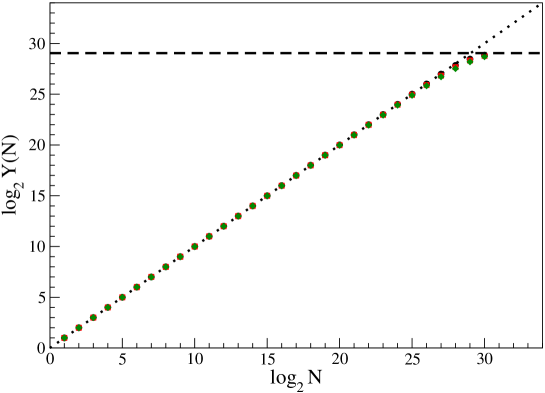
Figure 1: Log-log plot for distribution of base A. Circles, squares and diamonds are for capacity ($d_{0}$), information ($d_{1}$) and correlation ($d_{2}$) dimension, respectively (they strongly overlap). The dotted line has the slope coefficient equal 1, like for homogeneously or randomly distributed data points. The dashed line shows the saturation limit for the ordinate, due to the finite size of the data sample.

The resulting standard log-log plot used to extract generalized fractal dimensions for base A is shown in Fig. 1. Circles, squares and diamonds are for capacity ($d_{0}$), information ($d_{1}$) and correlation ($d_{2}$) dimension, respectively. In fact, the three symbols can hardly be distinguished, as they almost perfectly overlap. This excludes multifractality. Moreover, they are placed along the dotted line that has the slope coefficient equal $1.00$, like for homogeneously or randomly distributed data points. The dashed line shows the saturation limit for the ordinate, $\log_{2}(n_{dp})$, where $n_{dp}$ is the total number of data points due to the finite size of the sample [12]. Fig. 1 gives results for the base A, only. However, identical plots were obtained for all four bases, as well as for selected single chromosomes. Moreover, almost identical plots were obtained for randomly generated data samples of the same size.

Fig. 1 implies that the data set has integer (non-fractal) dimension precisely equal to 1.00. Clearly, due to the Hentschel-Procaccia inequality[14] $d_{q}=1.00$ for all $q<2$, as the function $d_{q})$ is monotonic. Calculations for higher values of $q$ were not performed because for very small $p_{i}(N)$ in sum in eq. 1 their high powers are beyond any reasonable compiler accuracy. Hence, one has to conclude that the spacing distribution of bases in HG does not show any trace of direct self-similarity, fractal or multifractal structure.

In this place, it is worth to remind, that within the 2-dimensional Chaos Game Representation (CGR) of DNA sequences [15] their fractal structure is well established by many authors (see e.g. [16]). Self-similarity in those cases is due to the special properties of the CGR transformation, that is a kind of recurrence plot technique [17]. These techniques are useful as randomness tests for random number generators [15], as well as stationarity tests for time series [9]. However, they do not imply self-similarity of the data sample by itself.

Even though the investigated data samples are not self-similar, and they were shown to have high entropy [18] — like random sequences — they are definitely not purely random. This will be shown in the following section. Moreover, even a highly structured data can resemble random series after compression, as the data compression algorithms increase the Shannon entropy.

4 Spacing distribution analysis

In this section we analyze the spacing distribution, $p(s)$, between bases of the same type. Here, spacing ($s$) is defined as the distance between two closest neighbors of the same type. For example, for the base A and the sequence AA the spacing of bases A is $s=1$. For the sequence AXA, where X is any base except A, the spacing is $s=2$ etc. In Figs. 2,3 the circles show (normalized) probabilities, $p(s)$, of a given spacing in the sample. In addition, we added a dotted line that corresponds to the uniform random distribution of bases,

$$p_{rand}(s)=1/3\times(3/4)^{s}\ ,\quad{\rm where}\ \sum_{s=1}^{s=\infty}p(s)=1\ .$$ (2)

For the HG data the spacing distribution has cutoff for $s_{max}$ that is at most of order $10^{3}$. The total number of occurrences of base A (and T) is about $5.5\times 10^{8}$ and for base C (and G) about $4.1\times 10^{8}$. In Fig. 2 plots are given for bases A and C, while in Fig. 3 for bases T and G. Both pairs of plots are similar, in accordance with the Chargaff’s rule. All probability distributions are normalized to unity to enable comparison of samples with different sizes.

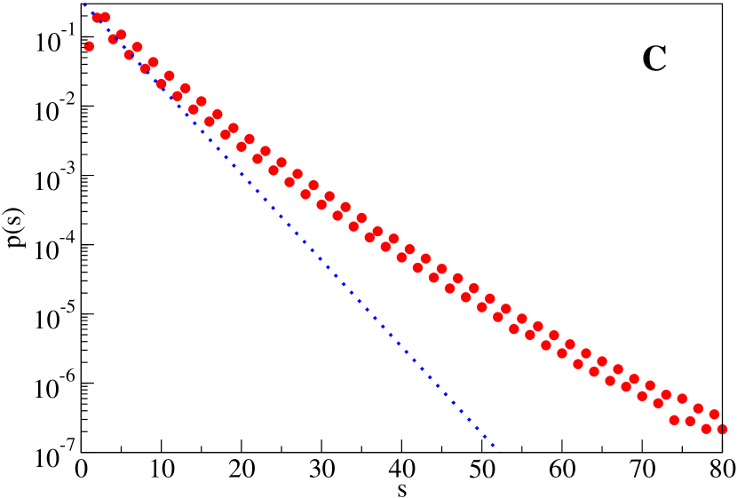
Figure 2: Normalized histogram of spacing distribution, $p(s)$, for bases A and C. The dotted line corresponds to a purely random distribution. Horizontal axis gives spacing distance and the vertical axis gives probability.

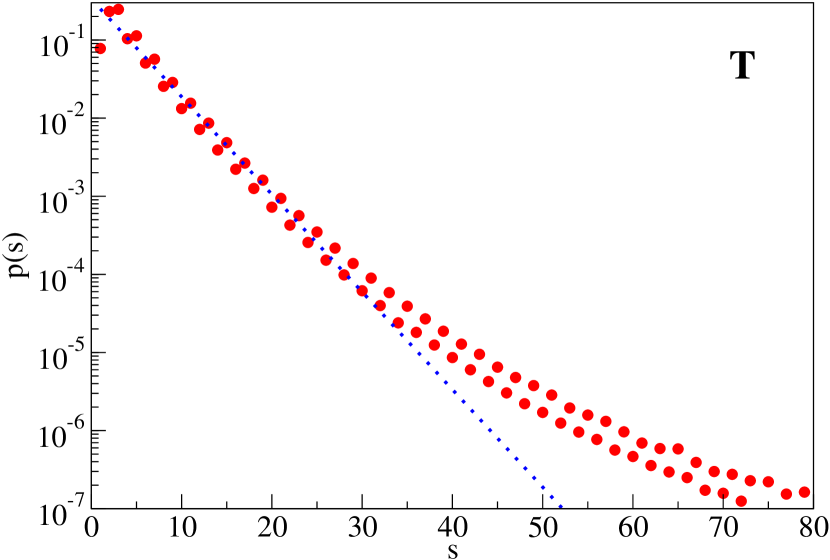
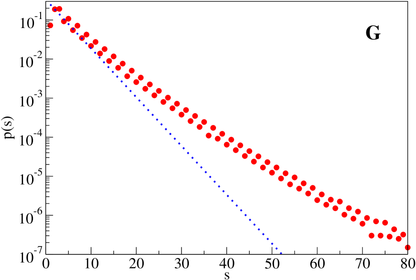
Figure 3: Normalized histogram of spacing distribution, $p(s)$, for bases T and G. The dotted line corresponds to a purely random distribution. Horizontal axis gives spacing distance and the vertical axis gives probability.

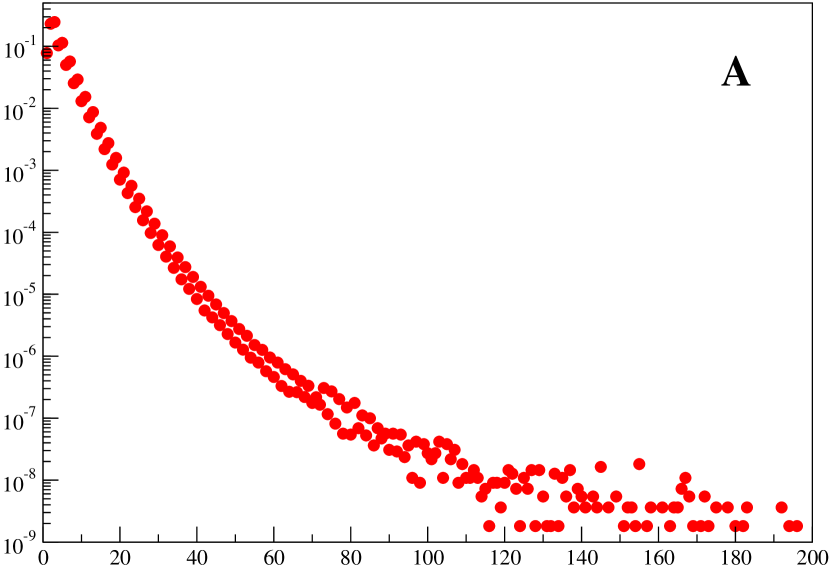
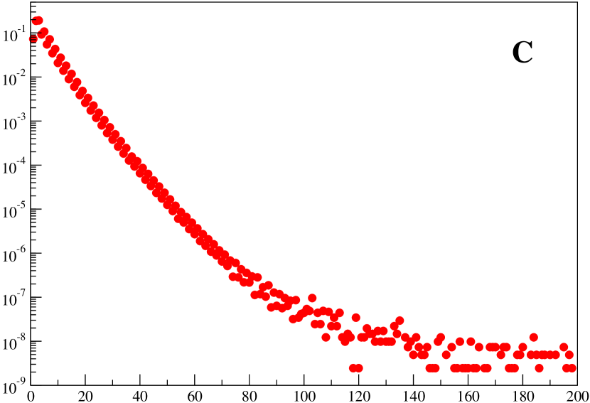
Figure 4: Normalized histogram of spacing distribution for bases A and C with tail up to $s=200$. Horizontal axis gives spacing distance and the vertical axis gives probability.

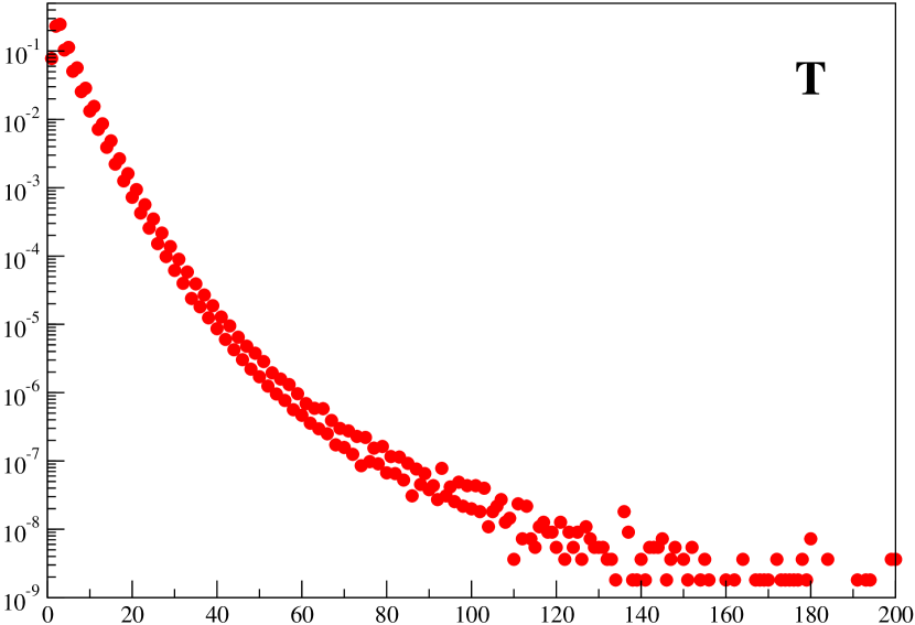
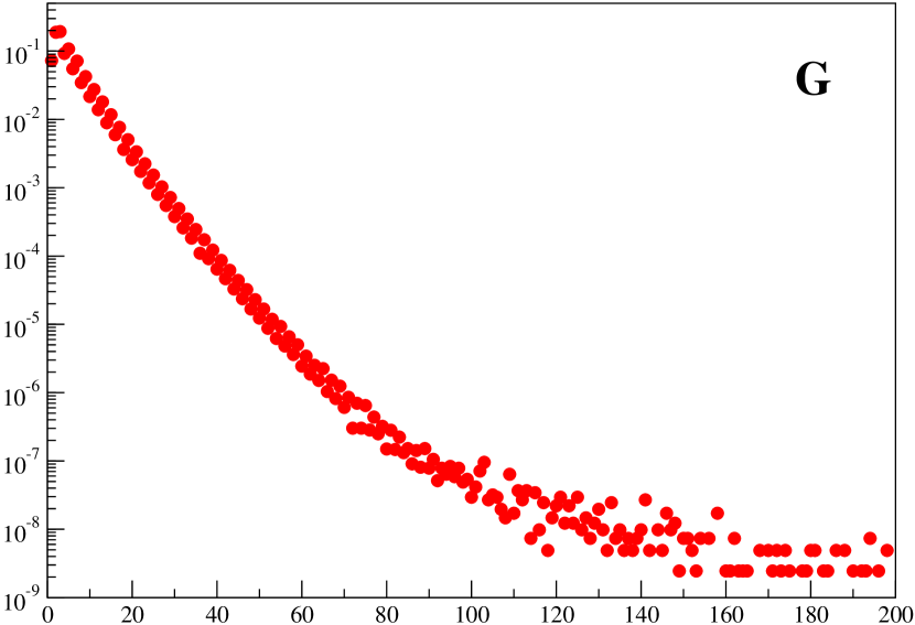
Figure 5: Normalized histogram of spacing distribution for bases T and G with tail up to $s=200$. Horizontal axis gives spacing distance and the vertical axis gives probability.

In Figs. 4 and 5 the tails of the histograms are shown up to $s=200$. Here, one can see that for larger spacings ($s$) the tail is getting fat and strongly deviates from exponential behavior. Also, one can see a kind of phase transition at $s_{2}\approx 80$ and the histograms’ bins are more randomly distributed. For $p(s)$ approaching $10^{-9}$ there are only single data points per bin and the statistics becomes less reliable. Hence, though the single events are up to $s\approx 1000$ they are not displayed. It should be stressed that fat tails are also common for self-organizing systems in economy, sociology etc., where long-range correlations (LRC) occur [9].

Closer examination of spacing distributions reveals several characteristic features that are listed below:

(i) For small spacing (about $s_{1}^{A}\approx 30$ for A and T bases, but $s_{1}^{C}<10$ for C and G bases) the distributions are quite close to the purely random distribution. However, for larger spacings the distributions strongly deviate form randomness.

(ii) The long tails of the distributions are strongly enhanced (’fat tails’) in comparison with the random distribution. This suggests strong long distance correlations.

(iii) In general, behavior of base A is similar as for base T, and the same holds for the (C,G) pair, though both pairs behave in different way. This can be viewed as another manifestation of the Chargraff’s rule.

(iv) For odd spacing ($s=3,5,7,...$) probability is higher than for their even predecessors. And the difference is slightly higher for (C,G) bases than for (A,T) bases. This is a kind of small high frequency oscillations in the distributions.

5 Discussion and Conclusion

It has been shown that the base spacing distribution in the HG is not random, though its high entropy. This is confirmed by the known fact that the nucleotide composition of the DNA sequence determines its spatial structure, function and stability of the spatial structure of the nucleic acid [19, 20, 21]

It has been found that the analyzed distribution has no fractal structure and for small spacings ($s<s_{1}$) it is close to random distribution (exponential decay). Analogous conclusion that the so-called random matches always dominate the distribution for small lengths has also been found recently for eukaryotic genomes [22], with similar suggested estimate, $s_{1}\approx 25$.

On the other hand, for larger spacing the distribution shows strong correlations and fat tails. Existence of LRC within the genome of living organism has immense importance in understanding the language of DNA sequences. However, the biological meaning of the LRC in DNA is, as yet, not clear. It is still an open and challenging problem. LRC has been suggested to be related to the duplication of DNA fragments Some authors claim that LRC occur only on intron containing DNA sequences, some however, that LRC do not distinguish between the intron and intronless DNA sequences. There have also been reports that LRC can be related to the nucleosomal structure and dynamics of the chromatin fiber. Our results are in agreement with conclusions reached by other authors, see e.g. [22, 23]. Moreover, the LRC have been shown important to the persistence of resonances of finite segments [24].

In addition, for large distances, $s>s_{2}\approx 80$, strong variability around any smooth interpolation was found. Variability of long nucleotide fragments is most likely responsible for structural variation, which is read by molecules interacting with DNA, which are conformationally sensitive. Attempts are made to analyze the variability of the DNA sequence in terms of structural variation resulting from variation at the sequence level by e.g. parametric and non-parametric entropy measures. Also, one can speculate, that relatively high entropy of the sequences reported previously [18] (and some similarity to random series) may be an effect of a kind of data compression algorithm.

Finally, the A-T and C-G bases have very similar distributions that is in accordance with the Chargaff’s rule. On the other hand, there is clear difference between the two pairs. The C-G bases have significantly higher probability for larger spacing (fatter tails). For $s=50$ the probability for C is about $10$ times higher. On the other hand, the tail for C is shorter and its maximum is slightly higher. Such behavior have also been found for genomes of other spacies [25].

References

- [1] E.D Green, J.D. Watson, F.S Collins, ”Human Genome Project: Twenty-five years of big biology”, Nature. 526 (2015) : 29–31.
- [2] B. Wilson, S.G. Nicholls, ”The Human Genome Project, and recent advances in personalized genomics”, Risk Manag Healthc Policy. 8 (2015) : 9.
- [3] S. Denisov, G. Bazykin, A. Favorov, A. Mironov, M. Gelfand, ”Correlated Evolution of Nucleotide Positions within Splice Sites in Mammals”, PLoS One. 10(12) (2015) :e0144388
- [4] J. Majewski, J. Ott, ”Distribution and characterization of regulatory elements in the human genome”, Genome Res. 12(12) (2002) :1827-36
- [5] E. Louie, J. Ott,J. Majewski, ”Nucleotide frequency variation across human genes”, Genome Res. 13(12) (2003) :2594-601
- [6] I.A. Babarinde, N. Saitou, ”Genomic Locations of Conserved Noncoding Sequences and Their Proximal Protein-Coding Genes in Mammalian Expression Dynamics”, Mol Biol Evol. ;33(7) (2016) :1807-17.
- [7] C.G. Sotero-Caio, R,N Platt RN, A. Suh, D.A. Ray, Evolution and Diversity of Transposable Elements in Vertebrate Genomes. Genome Biol Evol. 1;9(1) (2017) :161-177.
- [8] A.Z. Górski, J. Skrzat, ”Error estimation of the fractal dimension measurements of cranial sutures”, J. Anat. 208 (2006) 353-359.
- [9] A.Z. Górski, S. Drożdż, J. Speth, ”Financial multifractality and its subtleties: an example of DAX”, Physica A 316 (2002) 496-510.
- [10] www.ncbi.nlm.nih.gov, Genome Reference Consortium, Human Reference 38, FASTA file, p12, release Dec 27, 2017.
- [11] B.B. Mandelbrot, ”The Fractal Geometry of Nature” San Francisco, Freeman 1982.
- [12] A.Z. Górski, ”Pseudofractals and the box counting algorithm”, J. Phys. (GB) A34 (2001) 79337940.
- [13] A.Z. Górski, M. Stróż, P. Oświȩcimka, J. Skrzat, ”Accuracy of the box-counting algorithm for noisy fractals”, Int. J. Mod. Phys. 27 (2016) 1650112-1-12.
- [14] H.G.E. Hentschel, I. Procaccia, ”The infinite number of generalized dimensions of fractals and strange attractors”, Physica D 8 (1983) 435-444.
- [15] H.J. Jeffrey, ”Chaos game representation of gene structure”, Nucleic Acids Res. 18 (1990) 2163-2170.
- [16] P.A. Moreno, et al., ”The human genome: a multifractal analysis”, BMC Genomics 12 (2011) 506 1-17.
- [17] J.-P. Eckmann, S.O. Kamphorst, D. Ruelle, ”Recurrence plots of dynamical systems”, Europhys. Lett., 5(9) (1987) 973-977.
- [18] A.O. Schnitt, H.P. Herzel, ”Estimating the Entropy of DNA Sequences”, J. Theor. Biol. 1888 (1997) 369-377.
- [19] A.D. Vologodskii, M. Frank-Kamenetskii, ”Strong bending of the DNA double helix” Nucleic Acids Res. 41 (2013) : 6785–6792
- [20] A. Vologodskii, M.D. Frank-Kamenetskii, ”DNA melting and energetics of the double helix”, Phys Life Rev. 25 (2018) :1-21
- [21] A. Travers, ”DNA dynamics: bubble “n” flip for DNA cyclisation?”, Curr Biol. 15 (2015) : R377-9
- [22] F. Massip, M. Sheinman, S. Schbath, P.F. Arndt, ”How evolution of genomes is reflected in exact DNA match statistics”, Mol. Biol. Evol. 32 (2015) 524-535.
- [23] P.W. Messer, R. Bundschuh, M. Vingron, P.F. Arndt, ”Effects of long-range correlations in DNA sequence aligment score statistics”, J. Comput. Biol. 14 (2007) 655-668.
- [24] E.L. Albuquerque, M.S. Vasconcelos, M.L. Lyra, F.A. de Moura, ”Nucleotide correlations and electronic transport of DNA sequences”, Phys. Rev. E 71 (2005) 021910.
- [25] V. Afreixo, C.A. Bastos, A.J. Pinho, S.P. Garcia, P.J. Ferreira, ”Genome analysis with inter-nucleotide distances”, Bioinformatics 1 (2009) 3064-3070.
- [26]