PL-NMF: Parallel Locality-Optimized Non-negative Matrix Factorization

Abstract.

Non-negative Matrix Factorization (NMF) is a key kernel for unsupervised dimension reduction used in a wide range of applications, including topic modeling, recommender systems and bioinformatics. Due to the compute-intensive nature of applications that must perform repeated NMF, several parallel implementations have been developed in the past. However, existing parallel NMF algorithms have not addressed data locality optimizations, which are critical for high performance since data movement costs greatly exceed the cost of arithmetic/logic operations on current computer systems. In this paper, we devise a parallel NMF algorithm based on the HALS (Hierarchical Alternating Least Squares) scheme that incorporates algorithmic transformations to enhance data locality. Efficient realizations of the algorithm on multi-core CPUs and GPUs are developed, demonstrating significant performance improvement over existing state-of-the-art parallel NMF algorithms.

1. Introduction

Non-negative Matrix Factorization (NMF) is a key primitive used in a wide range of applications, including topic modeling (Shi et al., 2018; Kuang et al., 2015; Suh et al., 2017), recommender systems (Hernando et al., 2016; Aghdam et al., 2015; Zhang et al., 2006) and bioinformatics (Yang and Michailidis, 2015; Wang et al., 2013; Mejía-Roa et al., 2015). Given a non-negative matrix $A\in\mathbb{R}_{+}^{V\times D}$ and $K\ll\textrm{ min}(V,D)$, NMF finds two non-negative rank-K matrices $W\in\mathbb{R}_{+}^{V\times K}$ and $H\in\mathbb{R}_{+}^{K\times D}$, such that the product of $W$ and $H$ approximates $A$ (Lee and Seung, 2001):

(1) $$A\approx WH$$

NMF is a powerful technique for topic modeling. When $A$ is a corpus in which each document is represented as a collection of bag-of-words from an active vocabulary, the factor matrices $W$ and $H$ can be interpreted as latent topic distributions for words and documents.

Several algorithms have been proposed for NMF. They all involve repeated alternating update of some elements of $W$ interleaved with update of some elements of $H$, with imposition on non-negativity constraints on the elements, until a suitable error norm (either Frobenius norm or Kullback-Leibler divergence) is lower than a desired threshold. Various previously developed algorithms for NMF differ in the granularity of the number of elements of $W$ that are updated before switching to updating some elements of $H$. The focus of prior work has been to compare the rates of convergence of alternate algorithms and the parallelization of the algorithms. However, to the best of our knowledge, the minimization of data movement through the memory hierarchy, using techniques like tiling, has not been previously addressed. With costs of data movement from memory being significantly higher than the cost of performing arithmetic operations on current processors, data locality optimization is extremely important.

In this paper, we address the issue of data locality optimization for NMF. An analysis of the computational components of the FAST-HALS (Hierarchical Alternating Least Squares) algorithm for NMF (Cichocki and Phan, 2009), is first performed to identify data movement overheads. The associativity of addition is utilized to judiciously reorder additive contributions in updating elements of $W$ and $H$, to enable 3D tiling of a computationally intensive component of the algorithm. An analysis of the data movement overheads as a function of tile size is developed, leading to a model for selection of effective tile sizes. Parallel implementations of the new Parallel Locality-optimized NMF algorithm (called PL-NMF) are presented for both GPUs and multi-core CPUs. An experimental evaluation with datasets used in prior studies demonstrates significant performance improvement over state-of-the-art alternatives available for parallel NMF.

The paper is organized as follows. In the next section, we present the background on NMF and related prior work. In Section 3, we present the high-level overview of PL-NMF algorithm. Sections 4 and 5 demonstrate details of our PL-NMF for multi-core CPUs and GPUs. In Section 6, we systematically analyze the data movement cost for PL-NMF and original FAST-HALS algorithms. Section 7 presents determination of the tile sizes based on data movement analysis. In Section 8, we compare PL-NMF with existing state-of-the-art parallel implementations.

2. Background and Related Work

2.1. Non-negative Matrix Factorization Algorithms

NMF seeks to solve the optimization problem of minimizing reconstruction error between $A$ and the approximation $WH$. In order to measure the reconstruction error for NMF, Lee et al. (Lee and Seung, 2001) adopted various objective functions, such as the Frobenius norm given two matrices and Kullback-Leibler divergence given two probability distributions. The objective functions $D(A||WH)$ based on the Frobenius norm is defined in Equation 2.

(2) $$D_{F}(A||WH)=\frac{1}{2}||A-WH||_{F}^{2}=\frac{1}{2}\sum_{vd}\left(A_{vd}-(WH)_{vd}\right)^{2}$$

To efficiently minimize the objective functions (above), several variants of NMF algorithms have been developed: Multiplicative Update (MU), Additive Update (AU), Alternating Non-negative Least Squares (ANLS) and Hierarchical Alternating Least Squares (HALS). Table 1 describes the notations used in this paper.

Table 1. Common notations for NMF algorithms

Notation	Description
$A$	Non-negative matrix
$W$	Non-negative rank-$K$ matrix factor
$H$	Non-negative rank-$K$ matrix factor
$V$	Number of rows in $A$ and $W$
$D$	Number of columns in $A$ and $H$
$K$	Low rank

Multiplicative update (MU) and additive update (AU) proposed by Lee et al. (Lee and Seung, 2001) are the simplest NMF algorithms. The MU algorithm updates two rank-$K$ non-negative matrices $W$ and $H$ based on multiplicative rules and ensures convergence. MU strictly conforms to non-negativity constraints on $W$ and $H$ because the elements of $W$ and $H$ that have zero value will not be updated. Unlike MU algorithm, the AU algorithm updates $W$ and $H$ based on the gradient descent method and avoids negative update values using learning rate. However, some studies have reported that the use of MU and AU algorithms leads to weaknesses such as slower convergence and lower convergence rate (Gonzalez and Zhang, 2005; Lin, 2007; Kim and Park, 2008).

Alternating Non-negative Least Squares (ANLS) is a special type of Alternating Least Squares (ALS) approach. At each iteration, the gradients of two objective functions with respect to $W$ and $H$ are used to update each of $W$ and $H$ one after the other. Kim et al. (Kim and Park, 2011) proposed Alternating Non-negative Least Squares based Block Principle Pivoting (ANLS-BPP) algorithm. Under the Karush-Kuhn-Tucker (KTT) conditions, the ANLS-BPP algorithm iteratively finds the indices of non-zero elements (passive set) and zero elements (active set) in the optimal matrices until KTT conditions are satisfied. The values of indices that correspond to the active set will become zero, and the values of passive set are approximated by solving $min||A-WH||_{F}^{2}$ which is a standard Least Squares problem.

As an alternative to the basic ANLS approach, Cichocki et al. (Cichocki et al., 2007) proposed Hierarchical Alternating Least Squares (HALS), which hierarchically updates only one $k$-th row vector of $H\in\mathbb{R}_{+}^{K\times D}$ at a time and then uses it to update a corresponding $k$-th column vector of $W\in\mathbb{R}_{+}^{V\times K}$. In other words, HALS minimizes the $K$ set of two local objective functions with respect to $K$ row vectors of $H$ and $K$ column vectors of $W$ at each iteration. A standard HALS algorithm iteratively updates each row of $H$ and each column of $W$ in order within the innermost loop.

Based on the standard HALS algorithm, Cichocki et al. (Cichocki and Phan, 2009) further proposed the extended version of a new algorithm called FAST-HALS algorithm as described in Algorithm 1. Note that $H_{k}$ and $W_{k}$ indicate $k$-th row of $H$ and $k$-th column of $W$, respectively. FAST-HALS updates all rows of $H$ before starting the update to all columns of $W$, instead of alternately updating each row of $H$ and each column of $W$ at a time. Compared to MU algorithm, the FAST-HALS algorithm converges much faster and produces a better solution, while maintaining a similar computational cost as reported in (Kim and Park, 2011; Gillis, 2014). Interestingly, Kim et al. (Kim and Park, 2011) have shown that FAST-HALS has also been found to converge faster than their ANLS-BPP implementation on real-world text datasets: TDT2 and 20 Newsgroups, while maintaining the same convergence rate (see Figure 5.3 in Kim et al. (Kim and Park, 2011)).

2.2. Related Work on Parallel NMF

Since most of the variations of NMF algorithm are highly compute-intensive, many previous efforts have been made to parallelize NMF algorithms. As shown in Table 2, previous studies on parallelizing NMF can be broadly categorized into two groups based on implementation for multi-core CPUs (Battenberg and Wessel, 2009; Fairbanks et al., 2015; Dong et al., 2010; Liu et al., 2010; Liao et al., 2014; Kannan et al., 2016) versus GPUs (Lopes and Ribeiro, 2010; Mejía-Roa et al., 2015; Koitka and Friedrich, 2016). Furthermore, each study used various NMF algorithms for parallel implementations.

Table 2. Previous studies on parallelization of NMF

Author	Machine	Platform	Algorithm
Battenberg et al. (Battenberg and Wessel, 2009)	CPU	Shared-memory	MU
Fairbanks et al. (Fairbanks et al., 2015)	CPU	Shared-memory	ANLS-BPP
Dong et al. (Dong et al., 2010)	CPU	Distributed-memory	MU
Liu et al. (Liu et al., 2010)	CPU	Distributed-memory	MU
Liao et al. (Liao et al., 2014)	CPU	Distributed-memory	MU
Kannan et al. (Kannan et al., 2016)	CPU	Distributed-memory	ANLS-BPP
Lopes et al. (Lopes and Ribeiro, 2010)	GPU	Shared-memory	MU, AU
Koitka et al. (Koitka and Friedrich, 2016)	GPU	Shared-memory	MU, ALS
Mejía-Roa et al. (Mejía-Roa et al., 2015)	GPU	Distributed-memory	MU

2.2.1. Shared-Memory Multiprocessor

Battenberg et al. (Battenberg and Wessel, 2009) introduced parallel NMF using MU algorithm for audio source separation task. Fairbanks et al. (Fairbanks et al., 2015) adopted ANLS-BPP based NMF in order to find the structure of temporal behavior in a dynamic graph given vertex features. Both (Battenberg and Wessel, 2009) and (Fairbanks et al., 2015) developed the parallel NMF implementations on multi-core CPUs using Intel Math Kernel Library (MKL) along with shared-memory multiprocessor.

2.2.2. Distributed-Memory Systems

Dong et al. (Dong et al., 2010) demonstrated that MU algorithm and shared-memory based parallel implementation have a limitation of slow convergence. To overcome these problems, they devised a parallel MPI implementation of MU based NMF that improves Parallel NMF (PNMF) proposed by Robila et al. (Robila and Maciak, 2006). Different NMF algorithms have previously used tiling/blocking to minimize data movement. Dong et al. (Dong et al., 2010) partitioned the two factor matrices, W and H, into smaller blocks and each block is distributed to different threads. Each block simultaneously updates corresponding sub-matrices of the two matrices, and a reduction operation is performed by collective communication operations using Message Passing Interface (MPI). Similarly, Liu et al. (Liu et al., 2010) proposed matrix partition scheme that partitions the two factor matrices along the shorter dimension ($K$ dimension) instead of the longer dimensions ($V$ or $D$ dimensions). Therefore, each matrix is divided up to more partitions compared to partitioning along the longer dimension, so that the data locality is increased and the communication cost is decreased when performing the product of two matrices. Kannan et al. (Kannan et al., 2016) minimized the communication cost by communicating only with the two factor matrices and other partitioned matrices among parallel threads. Based on the ANLS-BPP algorithm, their implementation also reduced the bandwidth and data latency using MPI collective communication operations. Given an input matrix $A$ and two factorized matrices $W$ and $H$, they partitioned $W$ and $H$ into $P$ multiple blocks (tiles) across $V$ and $D$ dimensions which are the number of rows in $W$ and columns in $H$. Hence, the sizes of each block in $W$ and $H$ are ($V$/$P$)$\times$ $K$ and $K$ $\times$($D$/$P$), respectively. Doing so allows the matrix $A$ to be partitioned into $P$ tiles $\times$ $P$ tiles. Then $P$ different processors perform matrix multiplication with the different $P$ tiles of $W$ and $H$ simultaneously. This data partition scheme is appropriate for block-wise updates of $W$ and $H$ based on ANLS-BPP algorithm. Unlike ANLS-BPP algorithm, FAST-HALS requires column-wise/row-wise sequential updates because there is a data dependency between two consecutive columns/rows. Hence, FAST-HALS algorithm is not allowed to divide $W$ and $H$ across $V$ and $D$ dimensions. In our tiling approach, $W$ and $H$ are partitioned across $K$ dimension, and the sizes of each block in $W$ and $H$ are $V$ $\times$($K$/$P$) and ($K$/$P$)$\times$ $D$, respectively. Our key contribution is not tiling/blocking itself, but converting matrix-vector operations to matrix-matrix operations. Tiling enables us to do the latter.

2.2.3. GPU Platform

Lopes et al. (Lopes and Ribeiro, 2010) proposes several GPU-based parallel NMF implementations that use both MU and AU algorithms for both Euclidean and KL divergence objective functions. Mejía-Roa et al. (Mejía-Roa et al., 2015) presents NMF-mGPU that performs MU based NMF algorithm on either a single GPU device or multiple GPU devices through MPI for a large-scale biological dataset. Koitka et al. (Koitka and Friedrich, 2016) presents MU and ALS based GPU implementations binding to the R environment. To our knowledge, our paper is the first to develop FAST-HALS based parallel NMF implementation for GPUs.

3. Overview of Approach

In this section, we present a high-level overview of our approach to optimize NMF for data locality. We begin by describing the FAST-HALS algorithm (Cichocki and Phan, 2009), one of the fastest algorithms for NMF as demonstrated by previous comparison studies (Kim and Park, 2011). We analyze the data movement overheads from main memory, for different components of that algorithm, and identify the main bottlenecks. We then show how the algorithm can be adapted by exploiting the associativity of addition to make the computation effectively tileable to reduce data movement from memory, whereas the original form is not tileable.

3.1. Overview of FAST-HALS Algorithm

Algorithm 1 FAST-HALS algorithm

Input: $A\in\mathbb{R}_{+}^{V\times D}$: non-negative matrix, $\epsilon$: small non-negative quantity

1:  Initialize $W\in\mathbb{R}_{+}^{V\times K}$ and $H\in\mathbb{R}_{+}^{K\times D}$ with random non-negative numbers

2:  repeat

3:     // Updating H

4:     $R$ $\leftarrow$ $A^{T}W$

5:     $S$ $\leftarrow$ $W^{T}W$

6:     for k $=$ 0 to K $-$ 1 do

7:        $H_{k}$ $\leftarrow$ max$\left(\epsilon,H_{k}+R_{k}-H^{T}S_{k}\right)$

8:     end for

9:     // Updating W

10:     $P$ $\leftarrow$ $AH^{T}$

11:     $Q$ $\leftarrow$ $HH^{T}$

12:     for k $=$ 0 to K $-$ 1 do

13:        $W_{k}$ $\leftarrow$ max$\left(\epsilon,W_{k}Q_{kk}+P_{k}-WQ_{k}\right)$

14:        // Normalize $W_{k}$ column vector with $L_{2}-norm$

15:        $W_{k}\leftarrow\dfrac{W_{k}}{||W_{k}||_{2}}$

16:     end for

17:  until convergence

Algorithm 1 shows pseudo-code for the FAST-HALS algorithm (Cichocki and Phan, 2009) for NMF. It is an iterative algorithm that iteratively updates $H$ and $W$, fully updating all entries in $H$ (lines 4-8) and then updating all entries in $W$ (lines 10-15) during each iteration until convergence. While the updates to $H$ and $W$ are slightly different (due to normalization of $W$ after each iteration), each of the updates involves a pair of matrix-matrix products (lines 4/5 and 10/11 for $H$ and $W$, respectively) and a sequential loop that steps through features ($k$ loop) to update one row (column) of $H$($W$) at a time. The computation within these $k$ loops involves vector-vector operations and matrix-vector operations. From a computational complexity standpoint, the various matrix-matrix products and the sequential ($K$ times) matrix-vector products all have cubic complexity (O($N^{3})$ if all matrices are square and of side $N$). But as we show by analysis of data movement requirements in the next sub-section, the collection of matrix-vector products in lines 7 and 13 dominate. In the following sub-section, we present our approach to alleviating this bottleneck by exploiting the flexibility of instruction reordering via use of the associativity property of addition.

3.2. Data Movement Analysis for FAST-HALS Algorithm

The code regions with high data movement can be identified by individually analyzing each line in Algorithm 1. Lines 4 and 5 perform matrix multiplication. It is well known that $\frac{2MNK}{\sqrt{C}}$ is the highest order term in the number of data elements moved (between main memory and a cache of size $C$ words) for efficient tiled matrix multiplication of two matrices $A$, ($M\times K$) and $B$, ($K\times N$). Thus, the data movement costs associated with lines 4 and 5 are $\frac{2DKV}{\sqrt{C}}$ and $\frac{2KKV}{\sqrt{C}}$, respectively. The loop in line 6 performs matrix-vector multiplication and has an associated data movement cost of $K(3D+DK+K)$. Similar to lines 4 and 5, the data movement costs for lines 10 and 11 are $\frac{2VKD}{\sqrt{C}}$ and $\frac{2KKD}{\sqrt{C}}$, respectively. The loop in line 12 has an associated data movement cost of $K(VK+K+6V+1)$. The total data movement for Algorithm 1 is shown in Equation 3.

(3) $$K(K(V+D)(1+\frac{2}{\sqrt{C}})+\frac{4VD}{\sqrt{C}}+6V+3D+2K+1)$$

The main data movement overhead is associated with loops in lines 6 and 12. For example, the combined fractional data movement overhead of lines 7 (within loop in line 6) and 13 (within loop in line 12) is 91% for the 20 Newsgroups dataset. If the operational intensity (defined as the number of operations per data element moved) is very low, the performance will be bounded by memory bandwidth and thus will not be able to achieve the peak compute capacity. Due to its low operational intensity, the performance of Algorithm 1 is limited by the memory bandwidth. Thus, the major motivation for our algorithm adaptation is to achieve better performance by reducing the required data movement.

3.3. Overview of PL-NMF

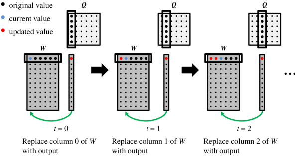
Figure 1. FAST-HALS: Update of $W$.

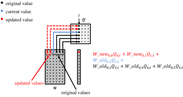
Figure 2. FAST-HALS: Updating a single element of $W$. The dash represents updated value.

In this sub-section, we describe how the FAST-HALS algorithm is adapted by exploiting the flexibility of changing the order in which additive contributions to a data element are made. Before describing the adaptation, we first highlight the interaction between different columns of $W$ in the original algorithm. Figure 1 depicts the update of $W$ which corresponds to the lines 12 to 16 in Algorithm 1.

In Algorithm 1, $t^{th}$ column of $W$ is updated as the product of $W$ with $t^{th}$ column of $Q$ which is a matrix-vector multiplication operation. Since the update to ${(t+1)}^{th}$ column depends on $t^{th}$ column, different columns ($t$: features) are updated sequentially. Let $W\_old$ represent the values at the beginning of the current outer iteration, and let $W\_new$ represent the values at the end of current outer iteration (updated values). Interaction between $W\_old$ and $W\_new$ is shown in Figure 2 which depicts the contributions from $W\_old$ and $W\_new$ to $W\_new_{i,t}$. $W\_new_{i,t}$ can be obtained by $\sum\limits_{j=0}^{t-1}W\_new_{i,j}\times Q_{j,t}+\sum\limits_{j=t}^{K-1}W\_old_{i,j}\times Q_{j,t}$.

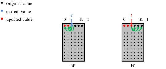
Figure 3. The contributions from $W_{0,t}$ to other elements.

Figure 3 shows the contributions of $W\_old_{i,t}$ and $W\_new_{i,t}$ to $W\_new_{i,*}$. $W\_old_{i,t}$ contributes to $W\_new_{i,j}$ $\forall j|j\leq t$, and $W\_new_{i,t}$ contributes to $W\_new_{i,j}$ where $\forall j|j>t$. In other words, the old value of column $t$ is used to update the columns to the left of $t$ (and self), and the new/updated value of column $t$ is used to update the columns to the right of column $t$.

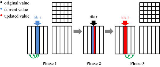
Figure 4. Overview of our approach for updating $W$.

Algorithm 2 Parallel CPU implementation for updating $W$

Input: $A\in\mathbb{R}_{+}^{V\times D}$: input matrix, $W\_old$ and $W\_new$: $V\times K$ non-negative matrix factor, $H$: $D\times K$ non-negative matrix factor, $T$: Tile size, $\epsilon$: small non-negative quantity, $\gamma$: total number of tiles

1:  $P$ $\leftarrow$ $AH^{T}$

2:  $Q$ $\leftarrow$ $HH^{T}$

3:  // Initialize $W\_new$ using $W\_old$ and $Q$

4:  for v $=$ 0 to V $-$ 1 do

5:     for k $=$ 0 to K $-$ 1 do

6:        $W\_new$[v][k] $\leftarrow$ $W\_old$[v][k] $\times$ $Q$[k][k]

7:     end for

8:  end for

9:  // Phase 1

10:  $\gamma$ $\leftarrow$ $K$ / $T$

11:  for tile_id $=$ 0 to $\gamma$ $-$ 1 do

12:     $W\_new$[0:$V$-1][0:(tile_id$\times$ $T$)-1] $-=$ dgemm($W\_old$[0:$V$-1][tile_id$\times~{}T$:((tile_id +1)$\times$ $T$)-1], $Q$[tile_id$\times$ $T$:((tile_id +1)$\times$ $T$)-1][0:(tile_id$\times$ $T$)-1])

13:  end for

14:  // Phase 2 & Phase 3

15:  for tile_id $=$ 0 to $\gamma$ $-$ 1 do

16:     // Phase 2

17:     for t $=$ tile_id $\times$ $T$ to (tile_id $+$ 1) $\times$ $T$ $-$ 1 do

18:        sum_square $\leftarrow$ 0

19:        #pragma omp parallel for reduction(+:sum_square)

20:        for v $=$ 0 to V $-$ 1 do

21:           sum $\leftarrow$ 0

22:           k $\leftarrow$ tile_id $\times$ $T$

23:           #pragma omp simd reduction(+:sum)

24:           for ; to t $-$ 1 do

25:              sum $\leftarrow$ sum $+$ $W\_new$[v][k] $\times$ $Q$[t][k]

26:           end for

27:           #pragma omp simd reduction(+:sum)

28:           for k $=$ t; to (tile_id $+$ 1) $\times$ $T$ $-$ 1 do

29:              sum $\leftarrow$ sum $+$ $W\_old$[v][k] $\times$ $Q$[t][k]

30:           end for

31:           $W\_new$[v][t] $\leftarrow$ max($\epsilon$, $W\_new$[v][t] $+$ $P$[v][t] $-$ sum)

32:           sum_square $\leftarrow$ sum_square $+$ $W\_new$[v][t] $\times$ $W\_new$[v][t]

33:        end for

34:        #pragma omp parallel for

35:        for v $=$ 0 to V $-$ 1 do

36:           $W\_new$[v][t] $\leftarrow$ $W\_new$[v][t] $/$ sqrt(sum_square)

37:        end for

38:     end for

39:     // Phase 3

40:     $W\_new$[0:$V$-1][(tile_id +1)$\times$ $T$:$K$-1] $-=$ dgemm($W\_new$[0:$V$-1][tile_id$\times$ $T$:((tile_id +1)$\times$ $T$)-1], $Q$[tile_id$\times$ $T$:((tile_id +1)$\times$ $T$)-1][(tile_id +1)$\times$ $T$:$K$-1])

41:  end for

If we partition $W$ into a set of column panels (tiles) of size $T$, the interactions between columns can be expressed in terms of tiles as depicted in Figure 4. Similar to individual columns, the old value of tile $\tau$ is used to update the columns to the left of $\tau$ (phase 1), and the new/updated value of tile $\tau$ is used to update the tiles to the right of tile $\tau$ (phase 3). The updates to different columns with a tile (phase 2) is done sequentially.

The contributions to tiles to the left of current tile $\tau$ can be done as $W\_new_{i,j}-=W\_old_{i,\tau\times T:((\tau+1)\times T)-1}\times Q_{\tau\times T:((\tau+1)\times T)-1,j}$ where $\forall j|j<\tau\times T-1$. Similarly, contributions to tiles to the right of current tile $\tau$ can be done as $W\_new_{i,j}-=W\_new_{i,\tau\times T:((\tau+1)\times T)-1}\times Q_{\tau\times T:((\tau+1)\times T)-1,j}$ where $\forall j|j>(\tau+1)\times T$. Both phases 1 and 3 can be performed using matrix-matrix operations which are known to have much better performance and lower data movement than matrix-vector operations. Note that the total number of operations in both the original formulation and our formulation are exactly the same.

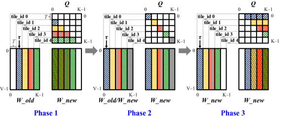
Figure 5. Computations of three phases for updating $W$.

4. Details of PL-NMF on Multicore CPUs and GPUs

4.1. Parallel CPU Implementation

Algorithm 2 shows our CPU pseudo-code for updating $W$. We begin by computing $AH^{T}$ (line 1). If $A$ is sparse, then the actual implementation uses mkl_dcsrmm() and cblas_dgemm() is used otherwise. Line 2 computes the $HH^{T}$ (using cblas_dgemm()). The $W$ values from the previous iteration are kept in $W\_old$. We maintain another data structure called $W\_new$ which represents the updated $W$ values. $W\_new$ is initialized by the loop in line 4. By using Equation 4, phase 1 is done by the loop in line 11. Figure 5 illustrates the actual computations of tiled matrix-matrix multiplications for three sequential phases, where $\tau$ denotes the index of the current tile and $T$ is the size of each tile. For example, at current tile $\tau$, phase 1 performs multiplication of the same colored/patterned two sub-matrices (tiles) in $W\_old$ and $Q$ to update the result matrix $W\_new$.

(4) $$\footnotesize\begin{multlined}W\_new[\,:\,,\,0:(\tau\times T)-1]\,-=\\ W\_old[\,:\,,\,(\tau\times T):((\tau+1)\times T)-1]\cdot\\ Q[(\tau\times T):((\tau+1)\times T)-1,\,0:(\tau\times T)-1]\end{multlined}W\_new[\,:\,,\,0:(\tau\times T)-1]\,-=\\ W\_old[\,:\,,\,(\tau\times T):((\tau+1)\times T)-1]\cdot\\ Q[(\tau\times T):((\tau+1)\times T)-1,\,0:(\tau\times T)-1]$$

The loop in line 17 performs phase 2 computations as formulated in Equation 5. In order to take advantage of the vector units, the loops in lines 24 and 28 are vectorized. Additionally, a column-wise normalization for $W\_new$ is performed within phase 2 (line 36).

(5) $$\footnotesize\begin{multlined}W\_new[\,:\,,\,(\tau\times T):((\tau+1)\times T)-1]\,-=\\ W[\,:\,,\,(\tau\times T):((\tau+1)\times T)-1]\cdot\\ Q[(\tau\times T):((\tau+1)\times T)-1,\,(\tau\times T):((\tau+1)\times T)-1]\\ +P[\,:\,,\,(\tau\times T):((\tau+1)\times T)-1]\end{multlined}W\_new[\,:\,,\,(\tau\times T):((\tau+1)\times T)-1]\,-=\\ W[\,:\,,\,(\tau\times T):((\tau+1)\times T)-1]\cdot\\ Q[(\tau\times T):((\tau+1)\times T)-1,\,(\tau\times T):((\tau+1)\times T)-1]\\ +P[\,:\,,\,(\tau\times T):((\tau+1)\times T)-1]$$

The matrix-matrix multiplication in line 40 corresponds to the phase 3 computations using Equation 6. As depicted in Figure 5, the tiles involving phase 3 and phase 1 computations are different from each other.

(6) $$\footnotesize\begin{multlined}W\_new[\,:\,,\,((\tau+1)\times T):K-1]\,-=\\ W\_new[\,:\,,\,(\tau\times T):((\tau+1)\times T)-1]\cdot\\ Q[(\tau\times T):((\tau+1)\times T)-1,\,((\tau+1)\times T):K-1]\end{multlined}W\_new[\,:\,,\,((\tau+1)\times T):K-1]\,-=\\ W\_new[\,:\,,\,(\tau\times T):((\tau+1)\times T)-1]\cdot\\ Q[(\tau\times T):((\tau+1)\times T)-1,\,((\tau+1)\times T):K-1]$$

Finally, our parallel CPU implementation completely substitutes lines 10 to 16 in Algorithm 1 for all lines in Algorithm 2. Similarly, $H$ will be updated in the same fashion as updating $W$ except for the normalization part.

4.2. Parallel GPU Implementation

Algorithm 3 GPU implementation of updating W on host

Input: $A\in\mathbb{R}_{+}^{V\times D}$: input matrix, $W\_old$ and $W\_new$: $V\times K$ non-negative matrix factor, $H$: $D\times K$ non-negative matrix factor, $T$: Tile size, $\epsilon$: small non-negative quantity, $\gamma$: total number of tiles

1:  $P$ $\leftarrow$ $AH^{T}$

2:  $Q$ $\leftarrow$ $HH^{T}$

3:  // Initialize $W\_new$ using $W\_old$ and $Q$

4:  init_W_new()

5:  // Phase 1

6:  $\gamma$ $\leftarrow$ $K$ / $T$

7:  for tile_id $=$ 0 to $\gamma$ $-$ 1 do

8:     $W\_new$[0:$V$-1][0:(tile_id$\times$ $T$)-1] $-=$ cublasDgemm($W\_old$[0:$V$-1][tile_id$\times$ $T$:((tile_id +1)$\times$ $T$)-1], $Q$[tile_id$\times$ $T$:((tile_id +1)$\times$ $T$)-1][0:(tile_id$\times$ $T$)-1])

9:  end for

10:  // Phase 2 & Phase 3

11:  for tile_id $=$ 0 to $\gamma$ $-$ 1 do

12:     // Phase 2

13:     for t $=$ tile_id $\times$ $T$ to (tile_id $+$ 1) $\times$ $T$ $-$ 1 do

14:        cudaMemset($sum\_square$,0)

15:        update_W_phase_2()

16:        __cudaDeviceSynchronize()

17:        update_W_norm()

18:        __cudaDeviceSynchronize()

19:     end for

20:     // Phase 3

21:     $W\_new$[0:$V$-1][(tile_id +1)$\times$ $T$:$K$-1] $-=$ cublasDgemm($W\_new$[0:$V$-1][tile_id$\times$ $T$:((tile_id +1)$\times$ $T$)-1], $Q$[tile_id$\times$ $T$:((tile_id +1)$\times$ $T$)-1][(tile_id +1)$\times$ $T$:$K$-1])

22:  end for

Algorithm 4 GPU implementation of update_W_phase_2 kernel

Input: $W\_old$, $W\_new$, $P$, $Q$, $sum\_square$, t, tile_id, $T$, $V$, $K$, $\epsilon$

1:  vId $\leftarrow$ blockIdx.x $\times$ blockDim.x $+$ threadIdx.x // threadID

2:  __shared__ $shared\_sum$[1024/32]

3:  sum_reduce = 0.0f

4:  if vId $<$ $V$ then

5:     sum = 0

6:     for k $=$ tile_id $\times$ $T$ to (tile_id $+$ 1) $\times$ $T$ $-$ 1 do

7:        if k $<$ t then

8:           sum $\leftarrow$ sum + $W\_new$[vId $+$ k $\times$ $V$][k] $\times$ $Q$[k $\times$ $K$ + t]

9:        else

10:           sum $\leftarrow$ sum + $W\_old$[vId $+$ k $\times$ $V$] $\times$ $Q$[k $\times$ $K$ + t]

11:        end if

12:     end for

13:     $W\_new$[vId $+$ t $\times$ $V$] $\leftarrow$ max($\epsilon$, $W\_new$[vId $+$ t $\times$ $V$] $+$ $P$[vId $+$ t $\times$ $V$] $-$ sum)

14:     sum_reduce $\leftarrow$ $W\_new$[vId $+$ t $\times$ $V$]

15:  end if

16:  sum_reduce $\leftarrow$ sum_reduce $\times$ sum_reduce

17:  // Warp-level reduction

18:  sum_reduce $\leftarrow$ warp_reduce(sum_reduce)

19:  // Block-level reduction

20:  if threadIdx.x % 32 == 0 then

21:     $shared\_sum$[threadIdx.x / 32] $\leftarrow$ sum_reduce

22:  end if

23:  __syncthreads()

24:  if threadIdx.x / 32 == 0 then

25:     sum_reduce $\leftarrow$ $shared\_sum$[threadIdx.x]

26:     sum_reduce $\leftarrow$ warp_reduce(sum_reduce)

27:  end if

28:  if threadIdx.x == 0 then

29:     atomicAdd ($sum\_square$, sum_reduce)

30:  end if

Algorithm 5 GPU implementation of update_W_norm kernel

Input: $W\_new$, $sum\_square$, t, $V$

1:  vId $\leftarrow$ blockIdx.x $\times$ blockDim.x $+$ threadIdx.x // threadID

2:  if vId $<$ $V$ then

3:     return

4:  end if

5:  $W\_new$[vId $+$ t $\times$ $V$] $\leftarrow$ $W\_new$[vId $+$ t $\times$ $V$] / sqrt($sum\_square$)

Similar to our CPU algorithm, our GPU algorithm also tries to minimize the data movement. Algorithm 3, 4 and 5 show the pseudo-code of our GPU algorithm. Since the overall structure of the GPU algorithm is similar to the CPU algorithm, this section only highlights the differences. Algorithm 3 runs on the host which is responsible for launching GPU kernels. The sparse matrix-dense matrix multiplication is implemented using cusparseDcsrmm(), and dense matrix-dense matrix multiplication is implemented using cublasDgemm().

Algorithm 4 shows the pseudo-code for phase 2. In GPUs, the reduction across $V$ (for normalization of $W$) can be performed using global memory atomic operations which are very expensive. Hence, our implementation uses efficient hierarchical reduction. The reduction within a thread block is done in 4 steps: i) in line 18, the reduction across the threads within a warp is done using efficient warp shuffling primitives, ii) all the threads with lane id 0 write the reduced value to shared memory (line 20), iii) in line 24, the first warp of the thread block loads the previously written values from shared memory and iv) all the threads in the first warp again performs warp reduction (line 26). In order to perform reduction across multiple thread blocks, we use atomic operations which is shown in line 29. Algorithm 5 shows the pseudo-code for normalization.

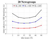
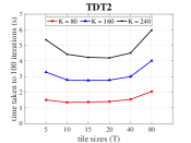
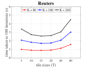
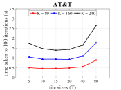
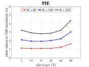
Figure 6. The time taken to reach 100 iterations when the tile size $T$ is varied for different $K$ on five datasets. Low-rank $K$ is set to 80, 160 and 240, and $T$ is varied for each $K$. X-axis: tile size; Y-axis: elapsed time to reach 100 iterations.

5. Modeling: Determination of the tile size

In this section, we first compare the data movement cost of our approach with original FAST-HALS algorithm. Then the data movement of our algorithm as a function of $T$ is developed to select effective tile sizes.

(7) $$\sum_{i=0}^{\frac{K}{T}-1}iVT^{2}(\frac{1}{T}+\frac{2}{\sqrt{C}})=VT^{2}(\frac{1}{T}+\frac{2}{\sqrt{C}})(\frac{K^{2}-KT}{2T^{2}})$$

(8) $$\sum_{i=0}^{\frac{K}{T}-1}T(VT+T+V)=\frac{K}{T}T(VT+T+V)$$

In our approach, $W$ is updated in three phases. Phases 1 and 3 can be implemented using matrix-multiplication, and the corresponding cost is shown in Equation 7, where $T$ represents the tile size and $C$ is the cache size. Phase 2 can be implemented using matrix-vector multiplication and the associated cost is shown in Equation 8. Since loading matrix $W$ dominates the data movement cost in phase 2, the cost of loading vectors can be ignored. Equation 9 shows the total data movement required for updating $W$.

(9) $$vol(T)=V(\frac{1}{T}+\frac{2}{\sqrt{C}})(K^{2}-KT)+\frac{K}{T}T(VT)$$

The cost of updating $H$ is similar to updating $W$. Compared to updating $W$, updating $H$ does not require accessing $Q$. In addition, since $H$ is not normalized, the cost associated with normalization is also not present.

The data movement cost of the original loop in line 12 in Algorithm 1 is $K(VK+K+6V+1)$. Hence, for the 20 Newsgroups dataset ($V$=11,314) with low rank $K$=160 on a machine with 35 MB cache, the data movement cost of original scheme is 300,525,600. However, in our scheme based on Equation 9, the cost is only 44,897,687 which is 6.7$\times$ lower than the original scheme.

The tile size $T$ affects the data movement volume and hence the performance. Equation 9 shows the data movement of our algorithm as a function of $T$. Consider the case when there is only one tile ($T=K$). In this case, there is no work associated with phase 1 (contributions to left) and phase 3 (contributions to the right) as the first term of Equation 9 will become zero. The total data movement of phase 2 is $VK^{2}$ which is very high. Now consider the other extreme where the tile size is 1 ($T=1$). In this case, phases 1 and 2 have very high data movement ($>VK^{2}$). Thus, when $T$ is high, the total data movements required for phases 1 and 3 are low, but phase 2 has high data movement. On the other extreme, when $T$ is low, the total data movements for phases 1 and 3 are high, but phase 2 has low data movement. Hence, we expect the combined data movement for all the phases to decrease as $T$ increases from 1 to some point and then the data movement will increase again as $T$ approaches $K$. Since performance is correlated with data movement, the performance as a function of tile size should show a similar trend and is shown in Figure 6.

(10) $$\frac{d(vol(T))}{dT}=T^{2}(\frac{2}{\sqrt{C}}-1)+K=0$$

(11) $$T=\sqrt{K-\frac{2}{\sqrt{C}}}$$

In order to build a model to determine the tile size for a given $K$, the derivative of Equation 9 with respect to $T$ is set it to zero (Equation 10). The solution to Equation 10 is shown in Equation 11. For a machine with cache size of 35 MB, the tile sizes computed by our model are 8.94, 12.64 and 15.49 for K=80, 160 and 240, respectively. Figure 6 shows that our model selected tile sizes that are optimal/near optimal.

6. Experimental Evaluation

This section compares the time to convergence and convergence rate of PL-NMF with various state-of-the-art techniques.

6.1. Benchmarking Machines

Table 3 shows the configuration of the benchmarking machines used for experiments. All the CPU experiments were run on an Intel Xeon CPU E5-2680 v4 running at 2.4 GHz with 128GB RAM. The GPU experiments were run on an NVIDIA Tesla P100 PCIE GPU with 16GB global memory.

Table 3. Machine configuration

Machine	Details
CPU	Intel(R) Xeon(R) CPU E5-2680 v4 (28 cores), 128GB ICC version 18.0.3
GPU	Tesla P100 PCIE (56 SMs, 64 cores/MP, 16GB Global Memory, 4 MB L2 cache) CUDA version 9.2.88

6.2. Datasets

For experimental evaluations we used three publicly available real-world text datasets – 20 Newsgroups, TDT23, Reuters3. In addition, in order to represent the audio-visual context analysis in social media platforms, we used two image datasets – AT&T and PIE. 20 Newsgroups, TDT2 and Reuters are sparse matrices, and AT&T and PIE are dense matrices. The 20 Newsgroups dataset contains a document-term matrix in bag-of-words representation associated with 20 topics. TDT2 (Topic Detection and Tracking 2) dataset is a collection of text documents from CNN, ABC, NYT, APW, VOA and PRI. Reuters dataset is a collection of documents from the Reuters newswire in 1987. Both AT&T and PIE datasets contain images of faces in dense matrix format. The size of each image in AT&T and PIE datasets is 92$\times$112 and 64$\times$64 pixels, respectively. Table 4 shows the characteristics of each dataset.

Table 4. Statistics of datasets used in the experiments. $V$ is the number of rows and $D$ is the number of columns in non-negative matrix $A$. For the text datasets, $V$ is the vocabulary size and $D$ is the number of documents.

Dataset	V	D	Total NNZ	Sparsity (%)
20 Newsgroups	26,214	11,314	1,018,191	99.6567
TDT2	36,771	10,212	1,323,869	99.6474
Reuters	18,933	8,293	389,455	99.7519
AT&T	400	10,304	4,121,478	0.0030
PIE	11,554	4,096	47,321,408	0.0080

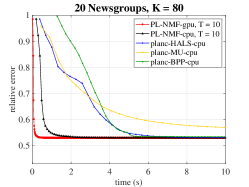
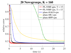
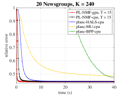
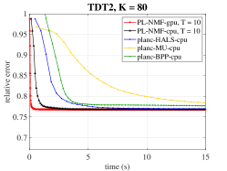
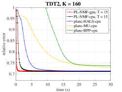
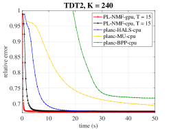
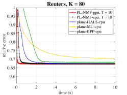
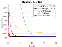
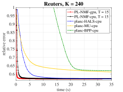
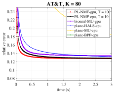
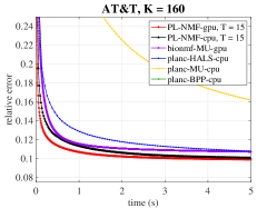
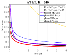
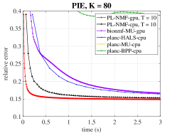
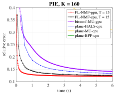
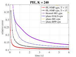
Figure 7. Relative objective value over time on five datasets. According to current model, the $T$ values for $K=$ 80, 160 and 240 are set to 10, 15 and 15, respectively. X-axis: elapsed time in seconds; Y-axis: relative error.

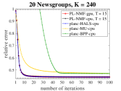
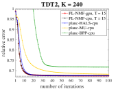
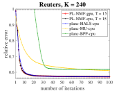
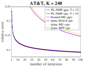
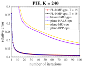
Figure 8. Comparison of convergence over iterations on five datasets, $K=$ 240 and $T=$ 15. X-axis: number of iterations; Y-axis: relative error.

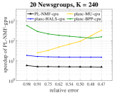
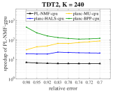
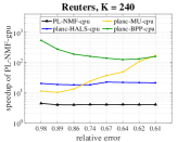
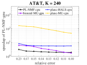
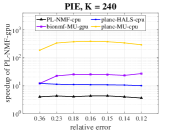
Figure 9. Speedup of PL-NMF-gpu over all CPU implementations on five datasets, $K=$ 240 and $T=$ 15.

6.2.1. NMF Implementations Compared

We evaluated PL-NMF on CPUs and GPUs with the state-of-the art parallel NMF implementations such as planc by Kannan et al. (Kannan et al., 2016; Fairbanks et al., 2015) and bionmf-gpu by Mejía-Roa et al. (Mejía-Roa et al., 2015). The four implementations used in our comparisons are as follows:

• planc-MU-cpu: planc’s OpenMP-based MU

• planc-HALS-cpu: planc’s OpenMP-based HALS

• planc-BPP-cpu: planc’s OpenMP-based ANLS-BPP

• bionmf-MU-gpu: bionmf-gpu’s GPU-based MU

All of the competing CPU implementations, including planc-MU-cpu, planc-HALS-cpu and planc-BPP-cpu, and our PL-NMF-cpu, used Intel’s Math Kernel Library (MKL) for all BLAS (Basic Linear Algebra Subprograms) operations. Similarly, all GPU implementations, including bionmf-MU-gpu and our PL-NMF-gpu, used NVIDIA’s cuBLAS library for all types of BLAS operations.

6.2.2. Evaluation Metric

In order to evaluate the accuracy of different NMF models, we used the relative objective function $\sqrt{\frac{\sum_{vd}(A_{vd}-(WH)_{vd})^{2}}{\sum_{vd}(A_{vd})^{2}}}$ suggested by Kim et al. (Kim and Park, 2011), where $A_{vd}$ and $(WH)_{vd}$ denote the values of each element in an input matrix $A\in\mathbb{R}_{+}^{V\times D}$ and an approximated matrix $(WH)\in\mathbb{R}_{+}^{V\times D}$. The capability of each NMF model in minimizing the objective function can be obtained by measuring relative changes of objective value over iterations.

6.3. Performance Evaluation

6.3.1. Convergence

Figure 7 shows the relative error as a function of elapsed time of various NMF implementations for different $K$ values. To ensure fairness, the number of threads in all CPU implementations were tuned per dataset and the best performing configuration was selected. For each dataset, the same randomly initialized non-negative matrices were used for all CPU and GPU implementations. Since the bionmf-MU-gpu implementation does not allow the input matrix to be sparse, we only compared our GPU implementation with bionmf-MU-gpu on AT&T and PIE dense image datasets. PL-NMF-cpu and PL-NMF-gpu consistently outperformed existing state-of-the-art CPU and GPU implementations on all datasets. As reported in previous studies, FAST-HALS produced a better convergence rate than other NMF variants. MU and ANLS-BPP algorithms suffered from a lower convergence rate on both sparse and dense matrices. As shown in Figure 8, planc-HALS-cpu was the only implementation which was able to maintain the same solution quality as ours. However, our implementation converged faster.

6.3.2. Speedup

Compared to the planc-HALS-cpu, our PL-NMF-cpu achieved 3.07$\times$, 3.06$\times$, 5.81$\times$, 3.02$\times$ and 3.07$\times$ speedup per iteration on the 20 Newsgroups, TDT2, Reuters, AT&T and PIE datasets with $K$ = 240, respectively. As the relative error reduction per iteration is vastly different between MU and FAST-HALS algorithms, measuring the speedup per iteration between bionmf-MU-gpu and PL-NMF-gpu is not a fair comparison.

Figure 9 depicts the speedup of our PL-NMF-gpu over all CPU implementations. The x-axis in Figure 9 is relative error, and the y-axis is the ratio of elapsed time for all CPU implementations to reach a relative error to elapsed time for PL-NMF-gpu to approach the same relative error. All of the points in Figure 9 are greater than one. This indicates that PL-NMF-gpu is faster than all of the competing implementations. For example, when the compared models, i.e., PL-NMF-cpu, planc-HALS-cpu, bionmf-MU-gpu and planc-MU-cpu, converged to 0.12 relative error, the parallel PL-NMF-gpu achieved 3.49$\times$, 9.74$\times$, 26.41$\times$ and 287.1$\times$ speedup on PIE dataset, respectively.

Table 5. Breakdown of elapsed time in seconds for updating $W$ on the 20 Newsgroups dataset. DMV: Iterative Dense Matrix-Vector Multiplications; DMM: Dense Matrix-Dense Matrix Multiplication; SpMM: Sparse Matrix-Dense Matrix Multiplication.

Sequential FAST-HALS NMF	elapsed time (s)	PL-NMF-cpu	elapsed time (s)
SpMM	0.048	SpMM	0.048
DMM	0.002	DMM	0.002
DMV	2.039	Phase 1	0.005
		Phase 2 & 3	0.026

Table 5 shows the breakdown of elapsed time for each step in updating $W$. Both sequential FAST-HALS NMF and PL-NMF-cpu implementations use the same mkl_dcsrmm() and cblas_dgemm() routines for SpMM and DMM operations. In Table 5, SpMM corresponds to line 10 in Algorithm 1 and line 1 in Algorithm 2, which computes the same $AH^{T}$. Similarly, DMM corresponds to line 11 in Algorithm 1 and line 2 in Algorithm 2, which performs the same $HH^{T}$. The difference of updating $W$ is that PL-NMF-cpu performs phases 1, 2 and 3 instead of iteratively performing DMV computations. As expected, the updating time of $W$ is considerably decreased in our PL-NMF-cpu algorithm, indicating that the reformulation of the core-computations to matrix-matrix multiplication shows the benefit of our approach.

7. Conclusion

In this paper, we developed a HALS-based parallel NMF algorithm for multi-core CPUs and GPUs. The data movement overhead is a critical factor that affects performance. This paper does a systematic analysis of data movement overheads associated with NMF algorithm to determine the bottlenecks. Our proposed approach alleviates the data movement overheads by enhancing data locality. Our experimental section shows that our parallel NMF achieves significant performance improvement over the existing state-of-the-art parallel implementations.

References

- (1)
- Aghdam et al. (2015) Mehdi Hosseinzadeh Aghdam, Morteza Analoui, and Peyman Kabiri. 2015. A novel non-negative matrix factorization method for recommender systems. Applied Mathematics & Information Sciences 9, 5 (2015), 2721.
- Battenberg and Wessel (2009) Eric Battenberg and David Wessel. 2009. Accelerating Non-Negative Matrix Factorization for Audio Source Separation on Multi-Core and Many-Core Architectures.. In ISMIR. 501–506.
- Cichocki and Phan (2009) Andrzej Cichocki and Anh-Huy Phan. 2009. Fast local algorithms for large scale nonnegative matrix and tensor factorizations. IEICE transactions on fundamentals of electronics, communications and computer sciences 92, 3 (2009), 708–721.
- Cichocki et al. (2007) Andrzej Cichocki, Rafal Zdunek, and Shun-ichi Amari. 2007. Hierarchical ALS algorithms for nonnegative matrix and 3D tensor factorization. In International Conference on Independent Component Analysis and Signal Separation. Springer, 169–176.
- Dong et al. (2010) Chao Dong, Huijie Zhao, and Wei Wang. 2010. Parallel nonnegative matrix factorization algorithm on the distributed memory platform. International journal of parallel programming 38, 2 (2010), 117–137.
- Fairbanks et al. (2015) James P Fairbanks, Ramakrishnan Kannan, Haesun Park, and David A Bader. 2015. Behavioral clusters in dynamic graphs. Parallel Comput. 47 (2015), 38–50.
- Gillis (2014) Nicolas Gillis. 2014. The why and how of nonnegative matrix factorization. Regularization, Optimization, Kernels, and Support Vector Machines 12, 257 (2014).
- Gonzalez and Zhang (2005) Edward F Gonzalez and Yin Zhang. 2005. Accelerating the Lee-Seung algorithm for non-negative matrix factorization. Dept. Comput. & Appl. Math., Rice Univ., Houston, TX, Tech. Rep. TR-05-02 (2005), 1–13.
- Hernando et al. (2016) Antonio Hernando, Jesús Bobadilla, and Fernando Ortega. 2016. A non negative matrix factorization for collaborative filtering recommender systems based on a Bayesian probabilistic model. Knowledge-Based Systems 97 (2016), 188–202.
- Kannan et al. (2016) Ramakrishnan Kannan, Grey Ballard, and Haesun Park. 2016. A high-performance parallel algorithm for nonnegative matrix factorization. In ACM SIGPLAN Notices, Vol. 51. ACM, 9.
- Kim and Park (2008) Hyunsoo Kim and Haesun Park. 2008. Nonnegative matrix factorization based on alternating nonnegativity constrained least squares and active set method. SIAM journal on matrix analysis and applications 30, 2 (2008), 713–730.
- Kim and Park (2011) Jingu Kim and Haesun Park. 2011. Fast nonnegative matrix factorization: An active-set-like method and comparisons. SIAM Journal on Scientific Computing 33, 6 (2011), 3261–3281.
- Koitka and Friedrich (2016) Sven Koitka and Christoph M Friedrich. 2016. nmfgpu4R: GPU-Accelerated Computation of the Non-Negative Matrix Factorization (NMF) Using CUDA Capable Hardware. R JOURNAL 8, 2 (2016), 382–392.
- Kuang et al. (2015) Da Kuang, Jaegul Choo, and Haesun Park. 2015. Nonnegative matrix factorization for interactive topic modeling and document clustering. In Partitional Clustering Algorithms. Springer, 215–243.
- Lee and Seung (2001) Daniel D Lee and H Sebastian Seung. 2001. Algorithms for non-negative matrix factorization. In Advances in neural information processing systems. 556–562.
- Liao et al. (2014) Ruiqi Liao, Yifan Zhang, Jihong Guan, and Shuigeng Zhou. 2014. CloudNMF: a MapReduce implementation of nonnegative matrix factorization for large-scale biological datasets. Genomics, proteomics & bioinformatics 12, 1 (2014), 48–51.
- Lin (2007) Chih-Jen Lin. 2007. Projected gradient methods for nonnegative matrix factorization. Neural computation 19, 10 (2007), 2756–2779.
- Liu et al. (2010) Chao Liu, Hung-chih Yang, Jinliang Fan, Li-Wei He, and Yi-Min Wang. 2010. Distributed nonnegative matrix factorization for web-scale dyadic data analysis on mapreduce. In Proceedings of the 19th international conference on World wide web. ACM, 681–690.
- Lopes and Ribeiro (2010) Noel Lopes and Bernardete Ribeiro. 2010. Non-negative matrix factorization implementation using graphic processing units. In International Conference on Intelligent Data Engineering and Automated Learning. Springer, 275–283.
- Mejía-Roa et al. (2015) Edgardo Mejía-Roa, Daniel Tabas-Madrid, Javier Setoain, Carlos García, Francisco Tirado, and Alberto Pascual-Montano. 2015. NMF-mGPU: non-negative matrix factorization on multi-GPU systems. BMC bioinformatics 16, 1 (2015), 43.
- Robila and Maciak (2006) Stefan A Robila and Lukasz G Maciak. 2006. A parallel unmixing algorithm for hyperspectral images. In Intelligent Robots and Computer Vision XXIV: Algorithms, Techniques, and Active Vision, Vol. 6384. International Society for Optics and Photonics, 63840F.
- Shi et al. (2018) Tian Shi, Kyeongpil Kang, Jaegul Choo, and Chandan K Reddy. 2018. Short-Text Topic Modeling via Non-negative Matrix Factorization Enriched with Local Word-Context Correlations. In Proceedings of the 2018 World Wide Web Conference on World Wide Web. International World Wide Web Conferences Steering Committee, 1105–1114.
- Smith et al. (2018) Tyler Michael Smith et al. 2018. Theory and practice of classical matrix-matrix multiplication for hierarchical memory architectures. Ph.D. Dissertation.
- Suh et al. (2017) Sangho Suh, Jaegul Choo, Joonseok Lee, and Chandan K Reddy. 2017. Local topic discovery via boosted ensemble of nonnegative matrix factorization. In Proceedings of the 26th International Joint Conference on Artificial Intelligence. AAAI Press, 4944–4948.
- Wang et al. (2013) Jim Jing-Yan Wang, Xiaolei Wang, and Xin Gao. 2013. Non-negative matrix factorization by maximizing correntropy for cancer clustering. BMC bioinformatics 14, 1 (2013), 107.
- Yang and Michailidis (2015) Zi Yang and George Michailidis. 2015. A non-negative matrix factorization method for detecting modules in heterogeneous omics multi-modal data. Bioinformatics 32, 1 (2015), 1–8.
- Zhang et al. (2006) Sheng Zhang, Weihong Wang, James Ford, and Fillia Makedon. 2006. Learning from incomplete ratings using non-negative matrix factorization. In Proceedings of the 2006 SIAM international conference on data mining. SIAM, 549–553.