Triplet harvesting in the polaritonic regime: a variational polaron approach

Abstract

We explore the electroluminescence efficiency for a quantum mechanical model of a large number of molecular emitters embedded in an optical microcavity. We characterize the circumstances under which a microcavity enhances harvesting of triplet excitons via reverse intersystem-crossing (R-ISC) into singlet populations that can emit light. For that end, we develop a time-local master equation in a variationally optimized frame which allows for the exploration of the population dynamics of chemically relevant species in different regimes of emitter coupling to the condensed phase vibrational bath and to the microcavity photonic mode. For a vibrational bath that equilibrates faster than R-ISC (in emitters with weak singlet-triplet mixing), our results reveal that significant improvements in efficiencies with respect to the cavity-free counterpart can be obtained for strong coupling of the singlet exciton to a photonic mode, as long as the singlet to triplet exciton transition is within the inverted Marcus regime; under these circumstances, the activation energy barrier from the triplet to the lower polariton can be greatly reduced with respect to that from the triplet to the singlet exciton, thus overcoming the detrimental delocalization of the polariton states across a macroscopic number of molecules. On the other hand, for a vibrational bath that equilibrates slower than R-ISC (i.e., emitters with strong singlet-triplet mixing), we find that while enhancemnents in photoluminiscence can be obtained via vibrational relaxation into polaritons, this only occurs for small number of emitters coupled to the photon mode, with delocalization of the polaritons across many emitters eventually being detrimental to electroluminescence efficiency. These findings provide insight on the tunability of optoelectronic processes in molecular materials due to weak and strong light-matter coupling.

I Introduction

The strong light-matter coupling (SC) or polaritonic regime reached with organic molecules embedded in confined electromagnetic environments, such as optical microcavities, has attracted considerable attention due to the possibilities it offers to the control of chemical processes at the molecular level Törmä and Barnes (2014); Ebbesen (2016); Ribeiro et al. (2018); Feist et al. (2018); Flick et al. (2018). In this regime, the interaction energy between the molecular ensemble and the photonic modes surpasses their respective linewidths, resulting in the formation of hybrid photon-matter excitations termed polaritons Hopfield (1958). The novel tunability of chemical dynamics and related processes afforded in the SC regime with organic molecules has been proven in photoisomerization Hutchison et al. (2012), excitation energy transfer Zhong et al. (2016); Du et al. (2018); Sáez-Blázquez et al. (2018), optical selection rules Neuman et al. (2018), exciton transport Feist and Garcia-Vidal (2015); Schachenmayer et al. (2015) and more recently triplet harvesting Kéna-Cohen and Forrest (2007); Stranius et al. (2018); Polak et al. (2018). The SC regime has not been exclusively harnessed at optical frequencies, as unique signatures of chemical control Thomas et al. (2016); Dunkelberger et al. (2016); Chervy et al. (2017) and nonlinear responses F. Ribeiro et al. (2018); Xiang et al. (2018) have also been demonstrated for molecular vibrational transitions coupled to a microcavity field.

Polariton setups have also emerged as promising candidates to boost the efficiency and versatility of light-emitting diodes (LEDs) Bajoni et al. (2008) and organic photodiodes (OPDs) Eizner et al. (2018). As a proof of concept, electrical injection of carriers into inorganic polariton architectures has been shown to modulate light-matter coupling Chakraborty et al. (2018), thus opening new avenues towards polariton-based optoelectronic switches. Similarly, organic LEDs have been demonstrated utilizing molecular dyes in the ultrastrong coupling regime Gubbin et al. (2014); Mazzeo et al. (2014); Genco et al. (2018) and it has been recently shown that materials operating in the latter can feature a complete inversion of molecular dark and light-emissive states Eizner et al. (2019). These exciting applications prompt the development of theoretical models to account for experimental observations of the molecular SC regime del Pino et al. (2015); Galego et al. (2016); Herrera and Spano (2016, 2017), as well as to rationally design new polaritonic setups that could enhance chemical processes of contemporary interest Galego et al. (2017); Martínez-Martínez et al. (2018).

In this article, we explore the triplet electroluminescence efficiency of a microcavity containing molecules which feature a range of electronic parameters and couplings to the condensed phase vibrational bath. Our model aims to describe polaritonic OLEDs like those reported in Tischler et al. (2005); Genco et al. (2018), so we consider that (optically dark) triplet excitons are generated upon electrical injection and the latter can transition into fluorescent singlet states that emit light. Our approach relies on a master equation operating in a variationally optimized polaron frame, originally introduced by Silbey and Harris Silbey (1984); Harris and Silbey (1985) with generalizations due to Pollock Pollock et al. (2013), Wu Wu et al. (2016), and their respective coworkers. The foundation of this method lies on the application of a unitary transformation to the total Hamiltonian which yields renormalized system and system-bath interactions that are weak enough to be perturbatively treated.

The outline of this article is summarized as follows. In section II, we introduce our quantum mechanical model and the variational approach to address its dynamics. Next, in section III, we give a formal definition of the triplet electroluminescence efficiency and describe our approach to calculate the time-evolution of populations in the relevant chemical states of the system. Then, in section IV, we apply our approach to systems in two regimes of coupling to vibrational degrees of freedom. In section V, we identify the main limitation that must be overcome to reach a polariton-enhanced triplet-harvesting regime and propose an approach to circumvent this drawback. Finally, in section VI we summarize our study and conclude with an outlook of how polaritons could enhance the optoelectronic properties of molecular materials.

II Theory

We consider an ensemble of $N$ identical molecules embedded in an optical microcavity and interacting with the electromagnetic modes supported by the latter; for simplicity, we describe a single photonic mode interacting with the molecular ensemble, a coarse-graining approximation which is based on the much larger density of states (DOS) of the molecular degrees of freedom compared to the photonic ones del Pino et al. (2015); Daskalakis et al. (2017). Thus, $N$ should not be interpreted as the total number of molecules in the cavity, but rather as the average number of molecules that couple to a single photon mode.

The Hamiltonian of our model can be written as

$$H= H_{S}+H_{B}+H_{S-B}+H_{ph}$$

$$+H_{S-ph}+H_{T}+H_{T-B}+H_{S-T}.$$ (1)

Each molecule is modeled as a three-level electronic system, namely a singlet electronic ground state and two excited states with singlet and triplet spin characters, respectively. The energetics of the latter are correspondingly described by $H_{S}$ and $H_{T}$. Assuming electrical pumping in the linear regime, we can restrict the Hamiltonian to the single excitation manifold such that,

$$H_{S} =\sum_{n=0}^{N-1}\epsilon_{S}|n\rangle\langle n|,$$ (2a)

$$H_{T} =\sum_{n=0}^{N-1}\epsilon_{T}|T_{n}\rangle\langle T_{n}|.$$ (2b)

Here, $|n\rangle$ ($|T_{n}\rangle$) denotes a localized singlet (triplet) exciton at the $n$th molecular site and $\epsilon_{S}$ ($\epsilon_{T}$) is the vertical singlet (triplet) electronic excitation energy, while ($\hbar=1$)

$$H_{B}=\sum_{v}\sum_{n=0}^{N-1}\omega_{v}b_{v,n}^{\dagger}b_{v,n}$$ (3)

accounts for the vibrational degrees of freedom in the condensed phase environment, where $b_{v,n}^{\dagger}$ ($b_{v,n}$) is the creation (annihilation) operator for an excitation in the $v$-th harmonic mode with frequency $\omega_{v}$ on site $n$. The mode-dependent singlet (triplet) vibronic couplings $g_{S}^{(v)}$ ($g_{T}^{(v)}$) are included in $H_{S-B}$ ($H_{T-B}$):

$$H_{S-B} =\sum_{v}\sum_{n}|n\rangle\langle n|g_{S}^{(v)}(b_{v,n}+\text{h.c.}),$$ (4a)

$$H_{T-B} =\sum_{v}\sum_{n}|T_{n}\rangle\langle T_{n}|g_{T}^{(v)}(b_{v,n}+\text{h.c.}).$$ (4b)

The singlet-triplet intersystem crossing electronic coupling is given by

$$H_{S-T}=V_{ST}\sum_{n}\left(|n\rangle\langle T_{n}|+\text{h.c.}\right).$$ (5)

Finally, the photonic microcavity degree of freedom is encoded in

$$H_{ph}=\omega_{ph}|G,1_{ph}\rangle\langle G,1_{ph}|,$$ (6)

where $|G,1_{ph}\rangle$ accounts for the state of all molecules in the electronic ground state and one excitation in the photonic mode and its interaction with singlet excitons (in the rotating wave approximation, RWA) is described by

$$H_{S-ph} =\sum_{n}g\left(|G,1_{ph}\rangle\langle n|+\text{h.c.}\right),$$ (7)

$g$ being a single-molecule dipolar coupling. To describe the emergent dynamics upon electrical pumping of the optically dark triplet states, we employ a variational polaron transformed master equation. The latter has proven to reproduce reliable quantum dynamics in a wide range of coupling strengths between electronic degrees of freedom and phononic reservoirs Lee et al. (2012), while being computationally inexpensive compared to more accurate approaches such as path integral Makri and Makarov (1995a, b), multi-configuration time-dependent Hartree Meyer et al. (1990); Beck et al. (2000), hierarchical equations of motion Ishizaki and Fleming (2009), linearized density matrix evolution Huo and Coker (2011), surface-hopping Tully (1990); Prezhdo and Rossky (1997); Subotnik et al. (2016) and exact factorization Hoffmann et al. (2018) formulations. In particular, we consider a similar multi-site approach to the one developed by Pollock and coworkers Pollock et al. (2013), who considered a variational polaron transformation to compute population dynamics in exciton networks with local phonon reservoirs. Furthermore, we adapt a generalization introduced by Wu and coworkers Wu et al. (2016) who treated the photon-exciton and exciton-vibration on equal footing to describe the photoluminiscence and vibrational dressing in polaritonic setups. As a first step towards the development of a master equation, the Hamiltonian in Eq. (1) is transformed to the so-called polaron frame, for which we introduce the unitary transformation $e^{P}$, where

$$P= \sum_{n=0}^{N-1}\sum_{v}|n\rangle\langle n|\left[\sum_{l}(b_{v,n+l}^{\dagger}-b_{v,n+l})\frac{f_{l}^{(v)}}{\omega_{v}}\right]$$ (8)

$$+\sum_{n=0}^{N-1}\sum_{v}|G,1_{ph}\rangle\langle G,1_{ph}|\left[(b_{v,n}^{\dagger}-b_{v,n})\frac{h^{(v)}}{\omega_{v}}\right]$$

$$+\sum_{n=0}^{N-1}\sum_{v}|T_{n}\rangle\langle T_{n}|(b_{v,n}^{\dagger}-b_{v,n})\frac{f_{T}^{(v)}}{\omega_{v}}$$

$$\equiv \sum_{n=0}^{N-1}\left[|n\rangle\langle n|\hat{D}_{S}^{(n)}+|G,1_{ph}\rangle\langle G,1_{ph}|\hat{D}_{ph}+|T_{n}\rangle\langle T_{n}|\hat{D}_{T}^{(n)}\right]$$

is partially based on previous works Wu et al. (2016); Zeb et al. (2018). According to the ansatz in Eq. (8), the electronic and photonic degrees of freedom are dressed with vibrational bath excitations to an extent quantified by the set of parameters $\{f_{l}^{(v)},f_{T}^{(v)},h^{(v)}\}$ which are variationally determined, as will be explained below. The summation over $l$ in Eq. (8) assumes that the vibrational deformation can be extended over all sites in the singlet excited manifold (large polaron limit) as a result of the interaction of all optically bright singlet excitons to the same photon mode. Since the electronic triplet states do not directly interact with the photonic mode, the vibrational deformation of the triplet excited manifold is expected to be more localized (small polaron limit). In the polaron frame we have

$$e^{P}He^{-P} =\tilde{H}_{0}+\tilde{H}_{I}+H_{B},$$ (9)

where

$$\tilde{H}_{0}= \sum_{n}\tilde{\epsilon}_{S}|n\rangle\langle n|+\sum_{n}\tilde{\epsilon}_{T}|T_{n}\rangle\langle T_{n}|+\tilde{\omega}_{ph}|G,1_{ph}\rangle\langle G,1_{ph}|$$

$$+g\eta_{S-ph}\sum_{n}\left(|n\rangle\langle G,1_{ph}|+\text{h.c.}\right)$$

$$+V_{ST}\eta_{ST}\sum_{n}\left(|n\rangle\langle T_{n}|+\text{h.c.}\right).$$

$$= \tilde{H}_{0,k=0}+\sum_{k\neq 0}\tilde{H}_{0,k}$$ (10)

and

$$\tilde{H}_{0,k=0}= \tilde{\epsilon}_{S}|k=0\rangle\langle k=0|+\tilde{\epsilon}_{T}|T_{k=0}\rangle\langle T_{k=0}|$$

$$+\tilde{\omega}_{ph}|G,1_{ph}\rangle\langle G,1_{ph}|$$

$$+\frac{\Omega}{2}\eta_{S-ph}\left(|k=0\rangle\langle G,1_{ph}|+\text{h.c.}\right)$$

$$+V_{ST}\eta_{ST}\left(|k=0\rangle\langle T_{k=0}|+\text{h.c.}\right),$$ (11a)

$$\tilde{H}_{0,k\neq 0}= \tilde{\epsilon}_{S}|k\rangle\langle k|+\tilde{\epsilon}_{T}|T_{k}\rangle\langle T_{k}|+V_{ST}\eta_{ST}\left(|k\rangle\langle T_{k}|+\text{h.c.}\right).$$ (11b)

In Eqs. (10-11) we introduced a delocalized Fourier basis for the singlet $|k\rangle=\frac{1}{\sqrt{N}}\sum_{n}e^{ikn}|n\rangle$ and triplet excitons $|T_{k}\rangle=\frac{1}{\sqrt{N}}\sum_{n}e^{ikn}|T_{n}\rangle$, with $k=\frac{2\pi}{N}$, $m=0,1,2,\dots,N-1$. In this basis, the state $|k=0\rangle$ couples to the photonic mode with a superradiantly enhanced strength given by $\sqrt{N}g=\Omega/2$. The renormalized on-site energies in (10) are given by

$$\tilde{\epsilon}_{S} =\epsilon_{S}+\sum_{v}\left(\sum_{l}\frac{f_{l}^{(v)2}}{\omega_{v}}-2g_{S}^{(v)}\frac{f_{0}^{(v)}}{\omega_{v}}\right)$$ (12a)

$$\tilde{\epsilon}_{T} =\epsilon_{T}+\sum_{v}\left(\frac{f_{T}^{(v)2}}{\omega_{v}}-2g_{T}^{(v)}\frac{f_{0}^{(v)}}{\omega_{v}}\right)$$ (12b)

$$\tilde{\omega}_{ph} =\omega_{ph}+\sum_{v}N\frac{h^{(v)2}}{\omega_{v}}$$ (12c)

and the renormalization constant $\eta_{ST}$ ($\eta_{S-ph}$) is the thermal average of the relative displacement operator between the singlet and triplet (photonic) harmonic potential energy surfaces,

$$\eta_{S-ph} =\langle e^{\hat{D}_{S}^{(n)}}e^{-\hat{D}_{ph}}\rangle$$

$$=\exp\left[-\frac{1}{2}\sum_{l,v}\left(\frac{(f_{l}^{(v)}-h^{(v)})^{2}}{\omega_{v}^{2}}\right)\coth(\beta\omega_{v}/2)\right],$$

$$\eta_{ST} =\langle e^{\hat{D}_{S}^{(n)}}e^{-\hat{D}_{T}^{(n)}}\rangle$$

$$=\exp\bigg{\{}-\frac{1}{2}\sum_{v}\bigg{[}\frac{(f_{0}^{(v)}-f_{T}^{(v)})^{2}}{\omega_{v}^{2}}$$

$$+\sum_{l\neq 0}\frac{|f_{l}^{(v)}|^{2}}{\omega_{v}^{2}}\bigg{]}\coth(\beta\omega_{v}/2)\bigg{\}},$$

where $\langle A\rangle=\frac{\text{Tr}_{B}\{Ae^{-\beta H_{B}}\}}{Z_{H_{B}}}$, $\text{Tr}_{B}\{\cdot\}$ denoting a trace over the vibrational degrees of freedom, $\beta$ being the inverse temperature, and $Z_{H_{B}}=\text{Tr}_{B}\{e^{-\beta H_{B}}\}$ being the vibrational partition function. Notice that by taking $f_{l}^{(v)}=g_{S}^{(v)}\delta_{l,0}$ in Eq. (12a), we recover the full-polaron transformation for the singlet excitation, and $R_{S}=-\lambda_{S}=-\sum_{v}(g_{S}^{(v)})^{2}/\omega_{v}$, where $\lambda_{S}$ is the reorganization energy of the singlet excited state. In Eqs. (10)–(11), we also introduced a partition of the Hamiltonian into the molecular contribution that is totally symmetric under site permutations $\tilde{H}_{0,k=0}$ and the non-totally-symmetric one $\sum_{k\neq 0}\tilde{H}_{0,k}$. Since $[\tilde{H}_{0,k=0},\sum_{k\neq 0}\tilde{H}_{0,k}]=0,$ the eigenstates of $\tilde{H}_{0}$ can be found by independent diagonalization of each contribution:

$$\tilde{H}_{0,k=0} =\tilde{\epsilon}_{\text{UP}}|\text{UP}\rangle\langle\text{UP}|+\tilde{\epsilon}_{\text{MP}}|\text{MP}\rangle\langle\text{MP}|+\tilde{\epsilon}_{\text{LP}}|\text{LP}\rangle\langle\text{LP}|,$$ (14)

where we define the upper (UP), middle (MP) and lower (LP) polariton states $|j\rangle=c_{S}^{j}|k=0\rangle+c_{T}^{j}|T_{k=0}\rangle+c_{ph}^{j}|G,1_{ph}\rangle$, $j=\text{UP},\thinspace\text{MP},\thinspace\text{LP}$. On the other hand,

$$\sum_{k\neq 0}\tilde{H}_{0,k}=\sum_{k}\Big{[}\tilde{\epsilon}_{+}|k^{(+)}\rangle\langle k^{(+)}|+\tilde{\epsilon}_{-}|k^{(-)}\rangle\langle k^{(-)}|\Big{]}$$ (15)

describes mixed singlet-triplet eigenstates $|k^{(\pm)}\rangle=c_{S}^{\pm}|k\rangle+c_{T}^{\pm}|T_{k}\rangle$ with no photonic component, whose eigenenergies are given by $\tilde{\epsilon}_{\pm}=\frac{\tilde{\epsilon}_{S}+\tilde{\epsilon}_{T}}{2}\pm\frac{1}{2}\sqrt{(\tilde{\epsilon}_{S}-\tilde{\epsilon}_{T})^{2}+4V_{ST}^{2}\eta_{ST}^{2}}$. These states are commonly known as dark or exciton reservoirs Agranovich et al. (2003); Litinskaya et al. (2004). For clarity, we refer to the highest (lowest) energy eigenstates in Eq. (15) as the upper (lower) dark states. Notice that since we are ignoring inter-site couplings, we neglect the dispersive character of the exciton in the calculation of the eigenenergies (15), a valid assumption in view of the flat exciton dispersion relation compared to the photonic one in the $k$ range of interest. The residual interaction Hamiltonian in Eq. (9) is

$$\tilde{H}_{I} =\tilde{V}_{S}+\tilde{V}_{T}+\tilde{V}_{ph}+\tilde{V}_{S-T}+\tilde{V}_{S-ph},$$ (16)

which has been written as a sum of different contributions defined as follows,

$$\tilde{V}_{S}= \sum_{v}\sum_{n}|n\rangle\langle n|\bigg{[}(g_{S}^{(v)}-f_{0}^{(v)})(b_{v,n}^{\dagger}+b_{v,n})$$

$$-\sum_{l\neq 0}f_{l}^{(v)}(b_{v,n+l}^{\dagger}+b_{v,n+l})\bigg{]},$$ (17a)

$$\tilde{V}_{T}= \sum_{v}\sum_{n}|T_{n}\rangle\langle T_{n}|\left[(g_{T}^{(v)}-f_{T}^{(v)})(b_{v,n}^{\dagger}+b_{v,n})\right],$$ (17b)

$$\tilde{V}_{ph}= -\sum_{v}h^{(v)}|G,1_{ph}\rangle\langle G,1_{ph}|\sum_{n}\left(b_{v,n}^{\dagger}+b_{v,n}\right),$$ (17c)

$$\tilde{V}_{S-T}= \sum_{n}V_{ST}\left[e^{\hat{D}_{S}^{(n)}-\hat{D}_{T}^{(n)}}-\eta_{TS}\right]|n\rangle\langle T_{n}|+\text{h.c.},$$ (17d)

$$\tilde{V}_{S-ph}= \sum_{n}g\left[e^{\hat{D}_{S}^{(n)}-\hat{D}_{ph}^{(n)}}-\eta_{S-ph}\right]|n\rangle\langle G,1_{ph}|+\text{h.c.}.$$ (17e)

The calculation of the parameters $\{f_{l}^{(v)},f_{T}^{(v)},h^{(v)}\}$ is carried out by taking advantage of the Feynman-Bogoliubov inequality $F\leq F^{\prime}_{0}+\langle\tilde{H}_{I}\rangle_{\tilde{H}_{0}^{\prime}}$ Silbey (1984); Harris and Silbey (1985), where $F$ ($F^{\prime}_{0}$) is the free energy of the system governed by $H$ ($\tilde{H}_{0}^{\prime}=\tilde{H}_{0}+H_{B}$) and $\langle A\rangle_{\tilde{H}_{0}^{\prime}}=\text{Tr}\{Ae^{-\beta\tilde{H}_{0}^{\prime}}\}[\text{Tr}\{e^{-\beta\tilde{H}_{0}^{\prime}}\}]^{-1}$ where $\text{Tr}\{\cdot\}$ denotes the trace over the eigenstates of $\tilde{H}_{0}^{\prime}$ . Notice that by construction $\langle\tilde{H}_{I}\rangle_{\tilde{H}^{\prime}_{0}}=0$, and the leading correction to the exact equilibrium reduced density matrix is $O(\tilde{H}_{I}^{2})$ Lee et al. (2012), which justifies the (second order) perturbative treatment in $\tilde{H}_{I}$. It follows that the parameters $\{f_{l}^{(v)},f_{T}^{(v)},h^{(v)}\}$ can be found by minimizing $F^{\prime}_{0}=-\beta^{-1}\text{Tr}\{e^{-\beta\tilde{H}_{0}}\}$, which amounts to solving $\frac{\partial F^{\prime}_{0}}{\partial f_{i}^{(v)}}=\frac{\partial F^{\prime}_{0}}{\partial h^{(v)}}=0$. In our calculations, we consider a continuum vibrational bath limit, which is described in terms of the spectral densities $J_{i}(\omega)=\sum_{v}|g_{v}^{i}|^{2}\delta(\omega-\omega_{v})=a_{i}\frac{\omega^{3}}{\omega_{c}^{2}}e^{-\omega/\omega_{c}}$, $i=S,T$, where $\omega_{c}$ is a cutoff frequency, and $a_{i}$ is the dimensionless parameter that encodes the strength of coupling between the excited electronic state with character $i$ to the vibrational bath. The computational details of the solution for $\{f_{l}^{(v)},f_{T}^{(v)},h^{(v)}\}$ are summarized in the Appendix A. In the discussion that follows, we focus on the calculation of the population dynamics of the chemically relevant species as well as of the electroluminescence efficiencies.

III Dynamics in the polaron frame and definition of triplet electroluminescence efficiency

The open-quantum system dynamics associated with the Hamiltonian in Eq. (1) can be described in terms of the time evolution of the reduced density matrix (RDM) $\rho(t)=\text{Tr}_{B}\{\rho_{tot}(t)\}$, ($\rho_{tot}(t)$ is the total density matrix), governed by the Liouville equation in the Schrödinger picture

$$\frac{d\rho(t)}{dt} =\mathcal{L}\rho(t)-\{\Gamma_{nrad}+\Gamma_{ph},\rho(t)\},$$

where $\mathcal{L}\rho(t)=-i\text{Tr}_{B}\{[H,\rho_{tot}(t)]\}$, and $\{\rho(t),\Gamma_{i}\}=\rho(t)\Gamma_{i}+\Gamma_{i}\rho(t)$; $\Gamma_{rad}$, $\Gamma_{nrad}$, $\Gamma_{ph}$ phenomenologically account for the dissipative processes associated with the radiative and nonradiative decay of excitons Rebentrost et al. (2009), and photonic leakage, respectively. We define the triplet electroluminescence efficiency

$$\epsilon=2\int_{0}^{\infty}\text{Tr}\left\{\Gamma_{ph}\rho(\tau)\right\}d\tau,$$ (18)

where the trace is taken over all the degrees of freedom, namely, the electronic, vibrational, and photonic. Eq. (18) is analogous to the integrated probability used to define the efficiency of energy trapping in chromophoric complexes Rebentrost et al. (2009), but in the present context, acquires the meaning of the efficiency of emission of a photon. Here, we define $\Gamma_{nrad}=\frac{k_{nrad}^{S}}{2}\sum_{n}|n\rangle\langle n|+\frac{k_{nrad}^{T}}{2}\sum_{n}|T_{n}\rangle\langle T_{n}|$ and $\Gamma_{ph}=\frac{\kappa}{2}|G,1_{ph}\rangle\langle G,1_{ph}|$, $k_{nrad}^{i}$ being the nonradiative decay rate of electronic state $i=S,T$, and $\kappa$ being the cavity photon leakage rate. Since

$$\text{Tr}\{\Gamma_{ph}\rho_{tot}(t)\}= \text{Tr}\{\Gamma_{ph}e^{-P}\tilde{\rho}_{tot}(t)e^{P}\}$$

$$= \text{Tr}\{\Gamma_{ph}\tilde{\rho}_{tot}(t)\},$$ (19)

$\epsilon$ is an invariant quantity under the polaron transformation. This last condition permits the computation of Eq. (18) in the polaron frame, where the time evolution of the polaron transformed RDM $\tilde{\rho}(t)=\text{Tr}_{B}\{\tilde{\rho}_{tot}\}$ can be described in terms of second-order perturbation theory on $\tilde{H}_{I}$ within the secular Born-Markov approximation. This procedure guarantees that the long-time evolution of the polaritonic system properly thermalizes into the reduced equilibrium state due to $\tilde{H}_{0}$ which, due to the optimization of the variational parameters according to the Feynman-Bogoliubov bound (see Sec. II), provides a good description of the equilibrium state of the full system involving electronic states, vibrations, and photon.

For the calculation of $\epsilon$, we assume that the initial RDM corresponds to an incoherent mixture of localized excitations in the triplet electronic manifold, i.e., $\sum_{n}\langle T_{n}|\tilde{\rho}(0)|T_{n}\rangle=1$, $\sum_{n}\langle T_{n}|\tilde{\rho}(0)|n\rangle=\sum_{n}\langle T_{n}|\tilde{\rho}(0)|G,1_{ph}\rangle=\sum_{n}\langle n|\tilde{\rho}(0)|n\rangle=\langle G,1_{ph}|\tilde{\rho}(0)|G,1_{ph}\rangle=0$. Under these assumptions, the initial RDM in the polaron frame can be written as

$$\vec{\tilde{\rho}}(0)\approx\begin{bmatrix}\langle\text{UP}|\tilde{\rho}(0)|\text{UP}\rangle\\ \langle\text{MP}|\tilde{\rho}(0)|\text{MP}\rangle\\ \langle\text{LP}|\tilde{\rho}(0)|\text{LP}\rangle\\ \sum_{k\neq 0}\langle k^{+}|\tilde{\rho}(0)|k^{+}\rangle\\ \sum_{k\neq 0}\langle k^{-}|\tilde{\rho}(0)|k^{-}\rangle\end{bmatrix}\approx\begin{bmatrix}0\\ 0\\ 0\\ |c_{T}^{+}|^{2}\\ |c_{T}^{-}|^{2}\end{bmatrix},$$ (20)

where the approximation is the result of considering a localized initial state, which in the delocalized polaron picture translates into the population distributed uniformly among the dark and polariton states. Since the former feature a larger DOS than the latter, the population is predominantly concentrated in the dark states. We can rewrite Eq. (18) as

$$\epsilon=\int_{0}^{\infty}\kappa P_{ph}\cdot\vec{\tilde{\rho}}(\tau)d\tau,$$ (21)

where the vector

$$P_{ph} =\begin{bmatrix}|c_{ph}^{UP}|^{2}&|c_{ph}^{MP}|^{2}&|c_{ph}^{LP}|^{2}&0&0\end{bmatrix}$$

accounts for the photonic character of the different chemical species that take part in the population dynamics. The time evolution of $\vec{\tilde{\rho}}(\tau)$ is described in terms of a Pauli master equation in the secular Markovian approximation, where

$$\frac{d\vec{\tilde{\rho}}(t)}{dt} =\mathcal{M}\vec{\tilde{\rho}}(t).$$ (22)

For simplicity in the calculations and interpretation, we consider the evolution of the total population in the dark state manifolds $\sum_{k\neq 0}\langle k^{\pm}|\tilde{\rho}(t)|k^{\pm}\rangle$ rather than dissected among the individual populations $\{\langle k^{\pm}|\tilde{\rho}(t)|k^{\pm}\rangle\}$. The matrix $\mathcal{M}$ is given by

$$\mathcal{M}_{ij}=\begin{cases}k_{i\leftarrow j}&i\neq j\\ -\sum_{l\neq i}k_{l\leftarrow i}-\kappa_{phot}|\langle i|G,1_{ph}\rangle|^{2}&i=j\\ -k_{nrad}^{T}\langle i|\mathcal{I}_{T}|i\rangle-k_{nrad}^{S}\langle i|\mathcal{I}_{S}|i\rangle\end{cases}$$ (23)

where $k_{j\leftarrow i}$ is the rate of transfer from the state/manifold $|i\rangle$ to $|j\rangle$, and $\mathcal{I}_{T}=\sum_{n}|T_{n}\rangle\langle T_{n}|$, $\mathcal{I}_{S}=\sum_{n}|n\rangle\langle n|$. Details of the calculation of the population transfer rates are included in the Appendix B. Using Eq. (22) together with Eq. (21), we have that

$$\epsilon =-\kappa P_{ph}\mathcal{M}^{-1}\vec{\tilde{\rho}}(0).$$ (24)

To get further insight into the contributions of the different pathways of population transfer to $\epsilon$, we consider a Green’s function partition approach Rebentrost et al. (2009), under which

$$\mathcal{M}^{-1}=\mathcal{M}_{npol}^{-1}-\mathcal{M}_{npol}^{-1}\mathcal{M}_{pol}\mathcal{M}^{-1},$$ (25)

where we let $\mathcal{M}=\mathcal{M}_{pol}+\mathcal{M}_{npol}$, $\mathcal{M}_{pol}$ being the rate matrix that accounts for the feed and depletion of polariton states only, which amounts to considering the rates $k_{i\leftarrow j}$ where either $i$ or $j\in\{|UP\rangle,|MP\rangle,|LP\rangle\}$ while setting the other entries of $\mathcal{M}$ to $0$. Using Eqs. (24) and (25),

$$\epsilon=\epsilon_{dir}+\epsilon_{indir}$$

where $\epsilon_{dir}=\kappa P_{ph}\mathcal{M}_{npol}^{-1}\mathcal{M}_{pol}\mathcal{M}^{-1}\vec{\tilde{\rho}}(0)$, $\epsilon_{indir}=-\kappa P_{ph}\mathcal{M}_{npol}^{-1}\vec{\tilde{\rho}}(0)$, and $\epsilon$ can be written as a sum of a contribution due to polariton-participating processes and another one where they do not play a role.

IV Results and discussion

Based on the approach above, we are particularly interested in the dependence of $\epsilon$ with Rabi energy $\Omega$ and detuning between the cavity photon and the vertical singlet energy transition $(\Delta=\omega_{ph}-\epsilon_{S})$, considering molecular emitters which feature different regimes of interaction with the vibrational bath degrees of freedom (DOFs). For that purpose, we introduce two cases based on parameters chosen to represent a wide range of organic molecular emitters.

First, we consider (large) strengths of coupling to the vibrational environment $a_{S}=10$, $a_{T}=15$, and a frequency cutoff $\omega_{c}=0.01$ eV. The corresponding reorganization energy of the singlet electronic state is given by $\lambda_{S}=\int_{0}^{\infty}\frac{J_{S}(\omega)}{\omega}d\omega=0.2$ eV and the analogous quantity for the triplet is $\lambda_{T}=\int_{0}^{\infty}\frac{J_{T}(\omega)}{\omega}d\omega=0.3$ eV. The assumption of a single vibrational reservoir coupled to both the singlet and triplet states allows for the calculation of the reorganization energy of the singlet-triplet transition $\lambda_{ST}$ (see Appendix A for details), which for this specific case amounts to 0.01 eV. For simplicity, we do not consider high frequency vibrational bath modes (those which feature frequencies $\omega\gg\beta^{-1}$) in our calculations. Furthermore, we assume an energy gap between the equilibrium vibrational configurations of the triplet and singlet $\Delta G=(\epsilon_{T}-\lambda_{T})-(\epsilon_{S}-\lambda_{S})=-0.1$ eV and a weak intersystem crossing coupling amplitude $V_{ST}=2\times 10^{-5}$ eV. These parameters are typical for organic molecules that undergo thermally activated delayed fluorescence (TADF) Chen et al. (2015); Yang et al. (2017); Peng et al. (2017), where the population in the dark triplet states transfers to the bright singlets, with a R-ISC rate that depends on a thermal energy barrier between the latter. We also consider a relatively slow nonradiative decay of the triplet $k_{nrad}^{T}=2\times 10^{-7}$ ps^-1 Yang et al. (2017). Since the characteristic timescale of relaxation of the vibrational environment $\omega_{c}^{-1}\ll\hbar/|V_{ST}|$, we expect a fast relaxation of the latter into its equilibrium configuration before R-ISC ensues, a scenario termed ’fast bath’ in the literature Lee et al. (2012). This is the behaviour expected in the limit $\Omega\rightarrow 0$ (small polaron formation before electronic transition) which was confirmed in our numerical calculations.

The second case we considered is the opposite to the previous one, in which the vibrational DOFs of the environment are sluggish in comparison to the R-ISC transition time scale ($V_{ST}\gg\omega_{c}$), a scenario identified as ’slow bath’ Lee et al. (2012), which corresponds to molecular emitters with sizable singlet-triplet mixing via spin-orbit coupling or hyperfine interaction. For this case, we also chose large strengths of coupling to the vibrational environment $a_{S}=10$, $a_{T}=30$, while setting a small cutoff frequency $\omega_{c}=5\times 10^{-3}$ eV (which translate into $\lambda_{S}=0.01$ eV, $\lambda_{T}=0.03$ eV and $\lambda_{ST}=0.1$ eV). Furtheremore, we set $V_{ST}=0.05$ eV and $\Delta G=-0.01$ eV, parameters that are qualitatively aligned with molecules that exhibit fast singlet-fission Yost et al. (2014), which exhibit large electronic couplings, comparable to the energy gaps between the singlet and the (two-body) triplet state. For this case, if $k_{nrad}^{T}$ is small as above, the cavity-free triplet electroluminescence efficiency $\epsilon\approx 1$ and placing it in the cavity is not productive; hence, we assume that the molecule is such that it features a fast nonradiative triplet decay $k_{nrad}^{T}=2\times 10^{-3}$ ps^-1 , such that we explore the possibility to outcompete it by cavity-assisted processes. The temperature $T=300$ K is assumed for both cases.

For reference, we computed electroluminescence efficiencies in the cavity-free (bare molecules) case which are $\epsilon=0.027$ for the fast bath case, and $\epsilon=0.062$ for the slow one. The latter are calculated using Eq. (18), substituting $\Gamma_{ph}$ with $\Gamma_{rad}=\frac{k_{rad}^{S}}{2}\mathcal{I}_{S}$ , where $k_{rad}^{S}=10^{-2}$ ps^-1, a typical fluorescence rate for organic molecules.

Upon coupling to a cavity photon mode, the emergent dynamics are changed as a result of the modification of the bare molecular energy landscape and the reorganization energies between the polariton states. In the polaron frame, the former contribution is encoded in the energy spectrum introduced in Eqs. (14-15), whereas the latter is accounted for in the reorganization energies $\lambda_{i-j}$, $i\neq j$, $i,j\in UP,MP,LP,\pm$, where the subindices $\pm$ denote ${|k^{\pm}\rangle}$ states (in our model, the reorganization energies $\lambda_{i-(\pm)}$ are independent of the momentum of the dark states). The polaron frame picture of the dynamics in both the slow and the fast bath case is schematically illustrated in Fig. 1 and the variation of the electroluminescence efficiency with $\Delta$ and $\Omega$ for the two different molecular emitter cases is shown in Fig. 2.

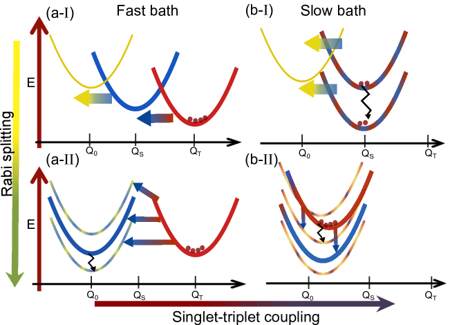
Figure 1: Scheme of polaron frame population dynamics which emerge upon injection of optically dark triplet excitons into molecules confined in an optical microcavity. For simplicity, we depict only one vibrational mode and represent its harmonic potential energy E as a function of its coordinate $Q$, in the photonic state (molecular ground state with one photon, yellow thin curve), and corresponding harmonic potential manifolds for singlet (blue thick curve) and triplet (red thick curve) excited states due to $N$ molecules. We consider molecules which feature (a) fast and (b) slow vibrational environment (see main text), compared to the R-ISC timescale defined by the singlet-triplet coupling $\hbar/V_{ST}$. For each case, we find qualitatively different mechanisms of population transfer among states for (I) weak and (II) strong light-matter coupling. The most significant mechanisms are depicted: multiphonon or Marcus-like processes with straight arrows, and single-phonon or Redfield-like processes with jagged ones.

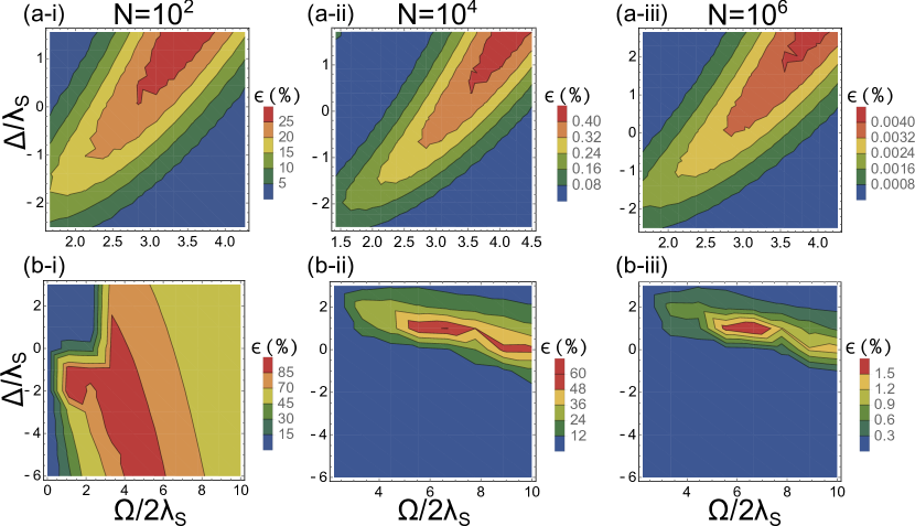
Figure 2: Triplet electroluminescence efficiency $\epsilon$ as a function of cavity detuning $\Delta=\omega_{ph}-\epsilon_{S}$ and Rabi splitting $\Omega$ for (a) the fast bath case, where vibrational equilibration occurs before a slow R-ISC and b) the slow bath case, where the opposite is true (where the emitters feature strong singlet-triplet mixing, see main text). The yields outside of the cavity are (a) $\epsilon=0.027$ for the fast bath and (b) $\epsilon=0.062$ for the slow one. The effective number of molecules per photon mode is: (i) $N=10^{2}$, (ii) $N=10^{4}$ and (iii) $N=10^{6}$.

For the discussion in this section, we limit ourselves to the $N=10^{2}$ case, postponing the important analysis of larger $N$ values for the next paragraphs.

Fast bath scenario.- For the fast bath molecule, we find that for weak light-matter couplings (Rabi splittings $\Omega\ll\lambda_{S}$), $\epsilon(\Delta,\Omega)$ is below the cavity-free scenario (for the resonant case $\Delta=0$, see inset in Fig. 3a). In the polaron frame, this observation can be explained in terms of thermally-activated transfer of population from the triplets to the photonic potential energy surface (PES) via the singlets (see Fig. 1a-I). Since this process involves passage through two thermal energy barriers, the time needed to reach the photonic PES is longer that the triplet lifetime and therefore $\epsilon\ll 1$. On the other hand, when $\Omega/2\lambda_{S}\approx 2/3$, our calculations predict an abrupt increase in $\epsilon$ (compare inset and main plot in Fig 3a). This is a manifestation of polaron decoupling Herrera and Spano (2017); Zeb et al. (2018) that is expected for sufficiently large Rabi splittings Herrera and Spano (2016); Zeb et al. (2018), under which the polariton PESs are essentially undisplaced with respect to the electronic ground PES. The intuition behind this decoupling is that the exchange of energy between photon and singlet excitons is much faster than that between vibrations and singlet excitons. Importantly, while this regime was previously predicted for $\Omega\gg\lambda_{S}$ Herrera and Spano (2018) for a single high-frequency mode, we hereby numerically demonstrate that this stringent condition can be relaxed to smaller Rabi splittings in the case of a continuum of low-frequency modes. In this polaron decoupling regime, our calculations predict that $\lambda_{(-)-UP}=\lambda_{(-)-MP}=\lambda_{(-)-LP}=\lambda_{(+)-(-)}>\lambda_{ST}$ [where the equality among the previous quantities is a result of the ansatz in Eq. (8), which for $\Omega/2\lambda_{S}>2/3$, corresponds to $f_{l}^{(v)}=f^{(v)}=O(\frac{g_{S}^{(v)}}{N})$, for all $l$. In other words, the singlet exciton PESs are negligibly displaced with respect to the ground state PES when $N$ is large]. As a consequence, the R-ISC energy barrier can either decrease or increase with respect to the bare molecules by tuning the Rabi splitting. In fact, we notice that as $\Omega$ increases (see Figs. 2a-i and 1a-II), $\epsilon$ increases and then decreases with respect to the cavity-free value, given that the smallest R-ISC to polariton energy barrier decreases and then increases as this rate goes from normal to inverted Marcus regimes. Notice that Fig. 3a only shows an increasing behavior in $\epsilon$ because the plotted range of Rabi splittings is small.

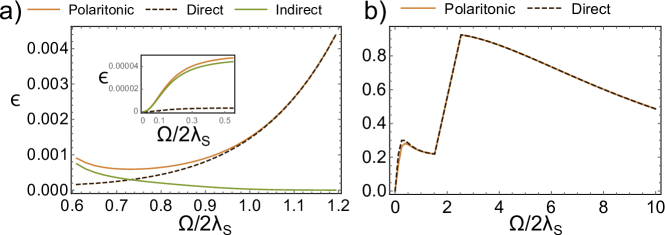
Figure 3: Partition of triplet electroluminescence efficiencies as a function of Rabi splitting $\Omega$ at light-matter resonance $\omega_{ph}=\epsilon_{S}$ (for $\Delta=0$) for a) a fast bath and b) a slow bath molecule; we show the case for $N=100$. The triplet electroluminescence efficiency $\epsilon$ (labeled as polaritonic) can be partitioned into a fraction that accounts for the direct and indirect population transfer from dark triplets into polaritons, where indirect means that population passes through other dark states before it reaches the polaritons. In b), we do not explicitly show the indirect contribution since it is negligible for featured Rabi splitting ranges. Inset in (a) zooms into smaller Rabi splitting ranges. For comparison, the yields outside of the cavity are (a) $\epsilon=0.027$ for the fast bath and (b) $\epsilon=0.062$ for the slow one.

Slow bath scenario.- For the slow bath case, we observe a significantly different $\epsilon(\Delta,\Omega)$. In Fig. [2b-i], we show that there is no need to invoke Rabi splittings beyond the reorganization energy to observe an enhancement in electroluminescence efficiency.

Similarly to the previous fast bath scenario, our calculations reveal two qualitatively different pictures of the population dynamics in the polaron frame depending on the magnitude of $\Omega$. For sufficiently weak light-matter coupling, the initial state is comprised of approximately equally populated lower and upper dark state manifolds since $|c_{S}^{+}|^{2}\approx|c_{S}^{-}|^{2}$ [see Eq. (20) and Fig. 1b-I], a consequence of the prevalence of the electronic coupling $V_{ST}$ over the weak coupling of the R-ISC transition to the phonon environment. In this regime, $\epsilon$ can be explained in terms of a Marcus picture where the photonic PES receives population from the upper and lower dark-state manifolds with a rate proportional to a diabatic coupling of order $|g|^{2}$, corresponding to single-molecule light-matter coupling [see Eq. (17e) and Fig. 1b-I]. High and small R-ISC energy barriers can be obtained by scanning across $\Delta$, thus decreasing and increasing $\epsilon$, respectively; for the computed range of $\Delta$ values, the dominant R-ISC pathway is the one starting from the upper dark states (they are closer in energy to the photonic PES, see Fig. 1b-I). In fact, for sufficiently small increase in $\Omega$, the triplet electroluminescence efficiency $\epsilon$ also rises because $|g|^{2}$ increases; see Fig. 3b, which shows a cut of $\epsilon$ at light-matter resonance $\Delta=0$. In this plot, this mechanism is operative up to a first maximum in $\epsilon$ at $\Omega\approx\lambda$, upon which light-matter coupling changes from weak to moderate and $\epsilon$ decreases. This effect can be understood as follows: as $\Omega$ increases, it can compete with $V_{ST}$, thus reducing the magnitude of the dressed $\tilde{V}_{ST}$, and concomitantly reducing the mixing between singlets and triplets. The result is that the lower and upper dark states become more triplet and singlet-like, respectively. Therefore, the initial triplet population has more probability of residing in the lower dark states, but these feature a much larger energy barrier to the photonic mode, thus leading to slower R-ISC and lower $\epsilon$.

Keeping our discussion around Fig. 3b, our model predicts a sharp change in the dynamics under strong light-matter coupling starting at $\Omega\approx 4\lambda_{S}$, with $\epsilon$ increasing with $\Omega$, featuring a second maximum in $\epsilon$ at $\Omega\approx 6\lambda_{S}$, and then decreasing for larger $\Omega$. An intriguing feature of this regime is that, for the chosen parameters, the upper and lower dark states have largely triplet and singlet characters, respectively; that is, the configuration of minimal energy of the vibrational DOFs coupled to the singlet and triplet states in the polaron frame is such that their energy ordering is inverted with respect to that in the original frame (Fig. 1b-II) where $\epsilon_{S}-\lambda_{S}>\epsilon_{T}-\lambda_{T}$. This effect is due to the slow relaxation of the bath that renders the vibrational dressing of the states at nonequilibrium nuclear configurations close to those accessed by vertical transitions from the ground state. Under these circumstances, population is primarily initialized in the upper dark states and transfers to the MP (Fig. 1b-II) which is closer in energy than the other polaritons or dark states. Notice that in contrast to the weak light-matter coupling case, MP has significant singlet, triplet, and photonic characters and the population transfer mechanism can be essentially dissected into sizable contributions from multiphonon (a Marcus-like contribution due to displacement between the upper dark states and MP harmonic potentials) and one-phonon (Redfield-like) processes. In our example, a steady boost in $\epsilon$ is given by the Redfield processes which dominate over the Marcus-like ones, given the large activation energy barriers to be surmounted in the latter. These Redfield processes are primarily due to the triplet character in both upper dark states and MP. After the second maximum in $\epsilon$, further increase of $\Omega$ leads to a phonon blockade and a concomitant decrease in $\epsilon$: the MP energy keeps lowering but no one-phonon process is available to mediate the transfer from the upper dark states (the vibrational DOS decreases exponentially as a function of frequency in our chosen spectral density).

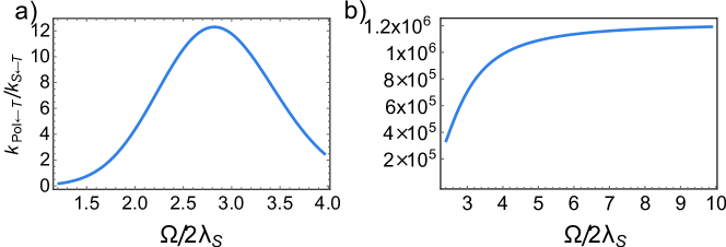
Figure 4: Relative R-ISC rates from triplet manifold to polariton states (at light-matter resonance $\omega_{ph}=\epsilon_{s}$) in the polaron frame with respect to the cavity-free case, for (a) the fast bath scenario and (b) the slow bath case, as a function of Rabi splitting, considering $N=10^{2}$. The profile observed in (a) (where the bare R-ISC rate is $k_{S\leftarrow T}=5.4\times 10^{-9}$ ps^-1), can be explained in terms of a multiphonon Marcus theory process from triplets to singlets (see Fig. 1a-II), where the lowest activation barrier between triplets and polaritons decreases (normal regime) and then increases (inverted regime). In (b) (where the bare R-ISC rate is $k_{S\leftarrow T}=4.6\times 10^{-6}$ ps^-1), the trend is different since the dominant R-ISC channel is a one-phonon process from triplets to the MP state (see Fig. 1b-II) and significantly depends on the triplet character of the latter. The asymptotic behavior of the rate reflects the increase in triplet character of the (MP) polariton state with Rabi splitting and the suppression of the energy gap between the latter and the triplet states. However, in this asymptotic limit, the photonic component of the MP vanishes and this channel does not longer contribute to the cavity electroluminescence efficiency. Finally, since the $k_{Pol\leftarrow T}$ rates shown here scale as $1/N$, the rates expected at different $N$ can be calculated by scaling the values displayed accordingly.

V The large N issue

So far, we have addressed the $N=100$ case in detail. In fact, strong light-matter coupling with such small number of molecular emitters has been reported using plasmonic nanoparticle environments Fofang et al. (2011); Bisht et al. (2018). However, most microcavity systems have much larger $N$ values. We thus proceed to comment on the $\epsilon$ behavior for increasing values of $N$, while keeping Rabi splittings $\Omega$ fixed (and hence energy barriers and energy differences between states, see Fig. 2). For weak light-matter coupling, both fast (a) and slow (b) baths yield insensitive changes of $\epsilon$ to increase of $N$. This is due to the fact that changing $N$ does not alter the energy barriers to be surmounted in the R-ISC process.

For strong light-matter coupling, the overall electroluminescence efficiency is damped as a result of the ratio of triplet to polariton states increasing. For the fast bath case (a), since both dark and polariton states feature the same reorganization energies in the polaron frame, $\epsilon$ is determined by the competition between the nonradiative triplet decay and transfer to the polariton state closer in energy, that is because the latter channel features a lower activation energy barrier compared to the dark states [see Fig. 1a-II)]. However, at light-matter resonance, the R-ISC rate to the final polariton state scales as $\frac{1}{N}$, given that the polariton is delocalized across $N$ singlets and only one of them can undergo coupling to a given triplet. Importantly, for $N\geq 10^{4}$ the rate of transfer to the polaritons falls below the cavity-free R-ISC rate for the entire $(\Delta,\omega)$ range displayed (see Fig. 2 top panels and 4a). The conclusion is similar for the slow bath case (b). While for small $N$ values, high efficiencies are obtained (see Fig. 2b-i and 2b-ii), the assistance of polariton modes decreases with increasing $N$. This is because the ratio of rates (dark states $\rightarrow$ polariton)/(polariton$\rightarrow$ dark states) scales as $\frac{1}{N}$ given the delocalization of the polariton state; this implies that the backward process polariton$\rightarrow$ dark states becomes more relevant as $N$ increases, an effect which is detrimental to $\epsilon$. Finally, the decrease of photon character in the MP for $\Delta<0$ [see Fig. 1b-II)] together with a fast back transfer to the denser manifold of upper dark states for larger $N$, explains the drop of $\epsilon$ at $\Delta<0$, specially for $N>10^{4}$ (see Fig. 2 lower panels and 4b).

Based on the discussion above, a pressing question is the characterization of an optimal scenario that overcomes the deleterious effects of cavity R-ISC rates as $N$ increases, the latter being as large as $10^{7}$ Daskalakis et al. (2017). Here, we propose a case where the energy tunability of the polaritons introduces an increase of many orders of magnitude relative to the cavity-free R-ISC rate, and this enhancement can outcompete the suppression due to the low polariton DOS. The scenario is built upon the fast bath case studied above, but assuming a sufficiently large singlet-triplet energy gap and weak couplings of the electronic states to the bath (small $a_{S}$ and $a_{T}$ parameters). Under these conditions, the reduced dynamics of transfer in the polaron frame in the cavity-free scenario corresponds to the inverted-Marcus regime (for the singlet to triplet transition), where the population of the triplet manifold needs to overcome an enormous energy barrier to reach the singlet state (see Fig. 5). Upon confinement to a microcavity, the emergent lower polariton could introduce a much smaller energy barrier from the triplet states. Our results and the precise parameters used in our calculations are shown in Fig. 5, which show that polariton-assistance introduces four orders of magnitude enhancement relative to the bare R-ISC rate. This mechanism of energy of activation reduction competing against delocalization is analogous to the one presented in our recent work on vibrational polaritons assisting thermally-activated reactions Campos-Gonzalez-Angulo et al. (2019).

On the other hand, we note that the polariton-assisted R-ISC rate is upper-bounded by $\frac{V_{ST}^{2}}{N}\sqrt{\frac{\pi\beta}{\lambda_{T-pol}}}$, which must be higher than $k_{nrad}^{T}$ to lead to harvesting of triplets. If we take $N=10^{6}$ , and use the parameters above for the fast bath scenario ($k_{nrad}=2\times 10^{-7}$ ps^-1), we need a very small $\lambda_{T-pol}=10^{-17}$ eV. Therefore, in order to obtain a sizable $\epsilon$, emitters with negligible couplings to a vibrational environment are required (small reorganization energies $\lambda_{ST}$ and $\lambda_{S}$); that is, poor R-ISC molecules (i.e., the opposite of TADF materials) will obtain most benefit from polaritonic effects. Whether this extreme possibility exists will be subject of future work.

For the slow bath case, there is no possibility to enhance electroluminescence for large $N$ because the associated R-ISC processes via polaritons happen via one-phonon vibrational relaxation (Redfield) processes, rather than multiphonon (Marcus) processes that exhibit exponential sensitivity on energy barriers. Hence, the only option for enhancement of electroluminescence for that case is to use samples with small $N$ values.

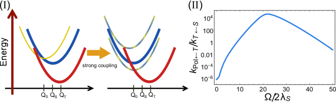
Figure 5: Ideal case to maximize the rate of transfer from the triplet state manifold (blue thick curve) to polariton states, with respect to the cavity free triplet-to-singlet (R-ISC) transfer rate. (I) Energy diagrams in the polaron frame. Left: a molecular emitter in which the singlet (blue) and triplet (red) states have similar equilibrium nuclear configurations and the dynamics between them falls within the Marcus inverted regime. (I) Right: upon strong coupling to a photon mode and in the polaron frame, the energy barrier between the triplet states and the lower polariton (in this case, the lower polariton) quickly decreases with Rabi splitting, giving rise to orders of magnitude increase in the $k_{T\rightarrow\text{LP}}$ rate, thus avoiding the wash-out effect of delocalization of the singlet of interest among $N$ molecules. (II) Cavity mediated R-ISC enhancement $k_{T\to\text{LP}}/k_{T\rightarrow S}$. Note that the cavity provides a realization of the various regimes of Marcus theory, from normal to inverted, as a function of Rabi splitting. The specific parameters for the vibrational bath are $a_{S}=0.5$, $a_{T}=1$ and $\omega_{c}=0.01$ eV (see Theory section), which accounts for a singlet reorganization energy $\lambda_{S}=0.01$ eV and $\lambda_{T}=0.02$ eV. We also assumed that the number of molecules per photon mode is $N=10^{6}$, $\Delta G=(\epsilon_{S}-\lambda_{S})-(\epsilon_{T}-\lambda_{T})=0.2$ eV, where we recall that $\epsilon_{S}$ ($\epsilon_{T}$) is the vertical singlet (triplet) transition energy; and the singlet-triplet electronic coupling $V_{TS}=1\times 10^{-5}$ eV.

VI Conclusions

In this article, we have developed a variational model for the prediction of electroluminescence efficiency of molecular emitters interacting with a photonic mode of a microcavity. The latter can describe the emergent dynamics on a range of Rabi splittings that extend from the weak to the the strong coupling regime.

Our calculations indicate that the main limitation to polariton-assist the electroluminescence process is the delocalized character of polaritons: the probability of a triplet state to R-ISC into the latter is strongly suppressed by a $\frac{1}{N}$ factor, similarly to results discussed in previous works Martínez-Martínez et al. (2018); Du et al. (2018); Eizner et al. (2019). There are two approaches that could overcome the detrimental delocalization effect and therefore introduce a polariton-enhanced electroluminescence with respect to the cavity-free scenario: 1) for fast and slow bath cases (i.e. for chromophores with weak and strong singlet-triplet mixing), as Figs. 2a-i and 2b-i show, strong coupling with a small number of molecules per photonic mode $N$ introduces significant electroluminescence yield enhancements with respect to the bare molecular case. This regime should be feasible in the context of plasmonic nanoparticles coated with organic dyes, where $N$ can be more than 3 orders of magnitude smaller than those needed in a microcavity to attain the strong coupling regime Fofang et al. (2011); Bisht et al. (2018); Munkhbat et al. (2018). 2) The second approach only works for the fast bath case and consists on tuning of polariton energies and taking advantage of the exponential sensitivity of R-ISC rates with respect to energy barriers. Therefore, a high thermal energy barrier for the R-ISC transition in the bare molecular case translates into the possibility of its partial or total reduction via a triplet to polariton R-ISC transition, thus potentially outcompeting the delocalization effect, and introducing a net electroluminescence enhancement. For a molecular emitter the previous requirement is equivalent to an inverted Marcus regime for the singlet$\rightarrow$triplet ISC transition. This mechanism is also reminiscent to a recently proposed catalysis of thermally-activated reactions under vibrational strong coupling, where a sufficient decrease in activation energy can outcompete the large activation entropy of the dark states Campos-Gonzalez-Angulo et al. (2019). An inverted Marcus regime being the ideal scenario to introduce polariton assistance has also been found in Martínez-Martínez et al. (2018) for singlet fission and in Semenov and Nitzan (2019), the latter in the context of a single-molecule charge transfer process assisted by a photon mode.

On the other hand, for the scenario of a slow vibrational bath, the efficiencies are largely determined by the energetic proximity of the polariton and dark state resonances. The increase of Rabi splitting in this case diminishes the rate of transition of the triplet to the polariton state closer in energy, because the vibrational DOS that can assist the transition decreases exponentially with the energy gap betwen them. Therefore, for the slow phonon bath scenario considered in this work, approach 1) is the only alternative to minimize the polariton-delocalization effect on efficiencies.

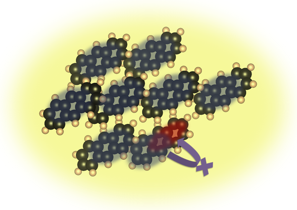
Figure 6: Scheme that illustrates the delocalization of a singlet electronic excitation (denoted as a faint blue on $N$ molecules) in a polariton mode under strong coupling to a confined electromagnetic environment (denoted as yellow). The localized nature of a triplet state (red) precludes a fast transfer to the polariton modes, in view of the local character of R-ISC and the dilution of probability of the R-ISC transition among $N$ molecules. As elaborated in section V of this article, this rate suppression can be overcome by 1) coupling fewer molecular emitters to each photon mode while preserving strong light-matter coupling (using e.g. plasmon nanoparticle systems); and/or ii) harnessing strong coupling of molecules with singlet$\rightarrow$triplet transition in the Marcus inverted regime, which feature very large R-ISC energy barriers, such that introduction of a polariton channel may decrease this barrier and possibly compete effectively against the many dark-state channels.

Appendix A. Variational optimization of polaron transformation

Formalism.— According to the Feynman-Bogoliubov bound described in section II, we are looking to variationally optimize the set $\{\vec{X}^{(v)}\}$ of $v$-dependent parameter vectors $\vec{X}^{(v)}\equiv[f_{0}^{(v)},f_{1}^{(v)},f_{T}^{(v)},h]$ that minimize the free energy due to $\tilde{H}_{0}^{\prime}$,

$$F_{0}^{\prime}(\{\vec{X}^{(v)}\}) =-\beta^{-1}\text{ln}\text{Tr}\left\{\exp\Big{[}-\beta\tilde{H}_{0}^{\prime}(\{\vec{X}^{(v)}\})\Big{]}\right\}$$

$$=-\beta^{-1}\text{ln}\Big{[}Z_{\tilde{H}_{0}}(\{\vec{X}^{(v)}\})\times Z_{H_{B}}\Big{]}.$$

Here, we have assumed $f_{1}^{(v)}=f_{2}^{(v)}=\dots=f_{N-1}^{(v)}\neq f_{0}^{(v)}$, which is equivalent to making a distinction between the vibrational deformation on a given molecular site and an indirect one induced via the photon on the rest of the sites, $f_{1}^{(v)}\equiv f_{l\neq 0}^{(v)}$. Furthermore,

$$Z_{\tilde{H}_{0}}(\{\vec{X}^{(v)}\}) =\sum_{p=+,-}(N-1)e^{-\beta\tilde{\epsilon}_{p}(\{\vec{X}^{(v)}\})}$$

$$+\sum_{q=\text{UP,MP,LP}}e^{-\beta\tilde{\epsilon}_{q}(\{\vec{X}^{(v)}\})},$$ (26a)

$$Z_{H_{B}} =N\prod_{v}(2\text{sinh}\frac{\beta\omega_{v}}{2})^{-1},$$ (26b)

are the corresponding polaritonic and vibrational partition functions. Since $Z_{H_{B}}$ does not depend on $\{\vec{X}^{(v)}\}$, we can minimize $F_{0}(\{\vec{X}^{(v)}\})=-\beta^{-1}\text{ln}Z_{\tilde{H}_{0}}(\{\vec{X}^{(v)}\})$ instead,

$$\nabla_{\vec{X}^{(v)}}F_{0} =\nabla_{\vec{Y}}F_{0}\cdot\nabla_{\vec{X}^{(v)}}\vec{Y}=0\hskip 10.00002pt\forall v,$$ (27)

where, using the chain rule, we have conveniently written $\vec{X}^{(v)}$ in terms of $\vec{Y}=[R_{S},R_{T},R_{ph},\eta_{ST},\eta_{S-ph}]$, where [see Eqs. (12)]

$$R_{S} =\sum_{v}\left(\sum_{l}\frac{f_{l}^{(v)2}}{\omega_{v}}-2g_{S}^{(v)}\frac{f_{0}^{(v)}}{\omega_{v}}\right),$$ (28a)

$$R_{T} =\sum_{v}\left(\frac{f_{T}^{(v)2}}{\omega_{v}}-2g_{T}^{(v)}\frac{f_{0}^{(v)}}{\omega_{v}}\right),$$ (28b)

$$R_{ph} =\sum_{v}N\frac{h^{(v)2}}{\omega_{v}}.$$ (28c)

The various terms in the $\nabla_{\vec{X}^{(v)}}\vec{Y}$ matrix are provided in Table 1.

TABLE 1. Derivatives $\frac{\partial y}{\partial x}$ where $y\in\{R_{S},R_{T},R_{ph},\eta_{ST},\eta_{S-ph}\}$ and $x\in\{f_{0}^{(v)},f_{1}^{(v)},f_{T}^{(v)},h\}$.
$x\backslash y$	$R_{S}$	$R_{T}$	$R_{ph}$	$\eta_{ST}$	$\eta_{S-ph}$
$f_{0}^{(v)}$	$\frac{2}{\omega_{v}}\left(f_{0}^{(v)}-g_{S}^{(v)}\right)$	$0$	$0$	$-\frac{(f_{0}^{(v)}-f_{T}^{(v)})}{\omega_{v}^{2}}\coth(\beta\omega_{v}/2)\eta_{ST}$	$-\frac{(f_{0}^{(v)}-h^{(v)})}{\omega_{v}^{2}}\coth(\beta\omega_{v}/2)\eta_{S-ph}$
$f_{l\neq 0}^{(v)}$	$\frac{2f_{1}^{(v)}}{\omega_{v}}$	$0$	$0$	$-\frac{f_{1}^{(v)}}{\omega_{v}^{2}}\coth(\beta\omega_{v}/2)\eta_{ST}$	$-\frac{(f_{1}^{(v)}-h^{(v)})}{\omega_{v}^{2}}\coth(\beta\omega_{v}/2)\eta_{S-ph}$
$f_{T}^{(v)}$	$0$	$\frac{2}{\omega_{v}}\left(f_{T}^{(v)}-g_{T}^{(v)}\right)$	$0$	$\frac{(f_{0}^{(v)}-f_{T}^{(v)})}{\omega_{v}^{2}}\coth(\beta\omega_{v}/2)\eta_{ST}$	$0$
$h^{(v)}$	$0$	$0$	$\frac{2Nh^{(v)}}{\omega_{v}}$	$0$	$\frac{(N-1)(f_{1}^{(v)}-h^{(v)})}{\omega_{v}^{2}}\coth(\beta\omega_{v}/2)\eta_{S-ph}$

For every $v$, Eq. (27) yields a set of four equations in terms of the four unknown entries of $\vec{X}^{(v)}$. Explicitly, for every $x\in\{f_{0}^{(v)},f_{1}^{(v)},f_{T}^{(v)},h\}$, we solve $\partial_{x}F_{0}=0$ for $x$, obtaining:

$$f_{0}^{(v)} =\frac{2g_{S}^{(v)}\omega_{v}\frac{\partial F_{0}}{\partial R_{S}}-h^{(v)}\frac{\partial F_{0}}{\partial\eta_{S-ph}}\coth(\beta\omega_{v}/2)\eta_{S-ph}-\frac{\partial F_{0}}{\partial\eta_{ST}}f_{T}^{(v)}\coth(\beta\omega_{v}/2)\eta_{ST}}{2\frac{\partial F_{0}}{\partial R_{S}}\omega_{v}-\eta_{S-ph}\coth(\beta\omega_{v}/2)\frac{\partial F_{0}}{\partial\eta_{S-ph}}-\frac{\partial F_{0}}{\partial\eta_{ST}}\eta_{ST}\coth(\beta\omega_{v}/2)},$$ (29a)

$$f_{1}^{(v)} =\frac{h^{(v)}\frac{\partial F_{0}}{\partial\eta_{S-ph}}\coth(\beta\omega_{v}/2)\eta_{S-ph}}{-2\omega_{v}\frac{\partial F_{0}}{\partial R_{S}}+\eta_{S-ph}\coth(\beta\omega_{v}/2)\frac{\partial F_{0}}{\partial\eta_{S-ph}}+\frac{\partial F_{0}}{\partial\eta_{ST}}\coth(\beta\omega_{v}/2)\eta_{ST}},$$ (29b)

$$f_{T}^{(v)} =\frac{2\frac{\partial F_{0}}{\partial R_{T}}g_{T}^{(v)}\omega_{v}-\frac{\partial F_{0}}{\partial\eta_{ST}}f_{0}^{(v)}\eta_{ST}\coth(\beta\omega_{v}/2)}{2\frac{\partial F_{0}}{\partial R_{T}}\omega_{v}-\frac{\partial F_{0}}{\partial\eta_{ST}}\coth(\beta\omega_{v}/2)\eta_{ST}},$$ (29c)

$$h^{(v)} =\frac{-[f_{0}^{(v)}+(N-1)f_{1}^{(v)}]\frac{\partial F_{0}}{\partial\eta_{S-ph}}\coth(\beta\omega_{v}/2)\eta_{S-ph}}{2\omega_{v}N\frac{\partial F_{0}}{\partial R_{ph}}-N\frac{\partial F_{0}}{\partial\eta_{S-ph}}\coth(\beta\omega_{v}/2)\eta_{S-ph}}.$$ (29d)

Analytical expressions for the derivatives $\partial_{y}F_{0}$ can be found in Appendix B. Next, we take the continuum limit of Eq. (29) by making the substitutions, $f_{l}^{(v)}\rightarrow f_{l}(\omega)$, $f_{T}^{(v)}\rightarrow f_{T}(\omega)$, $h^{(v)}\rightarrow h(\omega)$, and introducing the vibrational DOS $\mathcal{D}(\omega)=\omega\omega_{c}^{-2}e^{-\omega/\omega_{c}}$, upon which the bath spectral densities become $J_{i}(\omega)=a_{i}\frac{\omega^{3}}{\omega_{c}^{2}}e^{-\omega/\omega_{c}}=|g_{i}(\omega)|^{2}\mathcal{D}(\omega)$, $i=S,T$, where $|g_{i}(\omega)|^{2}=a_{i}\omega^{2}$ is the frequency-dependent vibronic-coupling intensity for each excitation. Since the spectral densities encode information on the geometries of the $S$ and $T$ states with respect to the ground molecular state, it is clear that they allow for the calculation of the spectral density for the singlet-triplet transition as $J_{ST}(\omega)=a_{ST}\frac{\omega^{3}}{\omega_{c}^{2}}e^{-\omega/\omega_{c}}$, $a_{ST}=(a_{T}^{1/2}\mp a_{S}^{1/2})^{2}$, as well as the corresponding reorganization energy $\lambda_{ST}=\int_{0}^{\infty}\frac{J_{ST}(\omega)}{\omega}d\omega$. Here, for each mode of frequency $\omega$, the minus sign should be chosen if the nuclear geometries of the $S$ and $T$ states shift in the same direction with respect to the ground molecular state, and the plus sign otherwise; we hereby assume the former, in light of geometries calculated for typical TADF molecules Peng et al. (2017). With these considerations, Eq. (29) can be manipulated to write $f_{1}$, $h$, and $f_{T}$ in terms of $f_{0}$ and to solve for $f_{0}$,

$$f_{0}(\omega) =\frac{\mathcal{R}(\omega)}{\mathcal{G}(\omega)+\frac{\partial F{}_{0}}{\partial\eta_{S-ph}}\eta_{S-ph}\coth(\beta\omega/2)(-2\frac{\partial F{}_{0}}{\partial R_{T}}\omega+\frac{\partial F{}_{0}}{\partial\eta_{ST}}\eta_{ST}\coth(\beta\omega/2))(1+(N-1)\mathcal{T}(\omega))\chi(\omega)},$$ (30a)

$$f_{1}(\omega) =\mathcal{T}(\omega)f_{0}(\omega),$$ (30b)

$$h(\omega) =-\Big{[}1+(N-1)\mathcal{T}(\omega)\Big{]}\chi(\omega)f_{0}(\omega),$$ (30c)

$$f_{T}(\omega) =\frac{2\frac{\partial F_{0}}{\partial R_{T}}g_{T}(\omega)\omega-\frac{\partial F_{0}}{\partial\eta_{ST}}\eta_{ST}\coth(\beta\omega/2)f_{0}(\omega)}{2\frac{\partial F_{0}}{\partial R_{T}}\omega-\frac{\partial F_{0}}{\partial\eta_{ST}}\coth(\beta\omega/2)\eta_{ST}}.$$ (30d)

These expressions depend on the following auxiliary functions,

$$\mathcal{R}(\omega) =2\omega\left[2\frac{\partial F{}_{0}}{\partial R_{S}}\frac{\partial F{}_{0}}{\partial R_{T}}g_{S}(\omega)\omega-\frac{\partial F{}_{0}}{\partial\eta_{ST}}\left(\frac{\partial F{}_{0}}{\partial R_{S}}g_{S}(\omega)+\frac{\partial F{}_{0}}{\partial R_{T}}g_{T}(\omega)\right)\eta_{ST}\coth(\beta\omega/2)\right],$$ (31a)

$$\mathcal{G}(\omega) =4\frac{\partial F{}_{0}}{\partial R_{S}}\frac{\partial F{}_{0}}{\partial R_{T}}\omega^{2}$$

$$\hskip 10.00002pt-2\left[\frac{\partial F{}_{0}}{\partial\eta_{S-ph}}\frac{\partial F{}_{0}}{\partial R_{T}}\eta_{S-ph}+\frac{\partial F{}_{0}}{\partial\eta_{ST}}\left(\frac{\partial F{}_{0}}{\partial R_{S}}+\frac{\partial F{}_{0}}{\partial R_{T}}\right)\eta_{ST}\right]\omega\coth(\beta\omega/2)$$

$$\hskip 10.00002pt+\frac{\partial F{}_{0}}{\partial\eta_{S-ph}}\frac{\partial F{}_{0}}{\partial\eta_{ST}}\eta_{S-ph}\eta_{ST}\coth(\beta\omega/2)^{2},$$ (31b)

$$\mathcal{T}(\omega) =\frac{\left(\frac{\partial F{}_{0}}{\partial\eta_{S-ph}}\right)^{2}\eta_{S-ph}^{2}\coth(\beta\omega/2)^{2}}{\mathcal{W}(\omega)},$$ (31c)

$$\mathcal{W}(\omega) =4N\frac{\partial F{}_{0}}{\partial R_{S}}\frac{\partial F{}_{0}}{\partial R_{ph}}\omega^{2}$$

$$\hskip 10.00002pt-2\left[\frac{\partial F{}_{0}}{\partial\eta_{S-ph}}\eta_{S-ph}\left(N\frac{\partial F{}_{0}}{\partial R_{ph}}+N\frac{\partial F{}_{0}}{\partial R_{S}}\right)+N\frac{\partial F{}_{0}}{\partial\eta_{ST}}\frac{\partial F{}_{0}}{\partial R_{ph}}\eta_{ST}\right]\omega\coth(\beta\omega/2)$$

$$\hskip 10.00002pt+\frac{\partial F{}_{0}}{\partial\eta_{S-ph}}\eta_{S-ph}\left(\frac{\partial F{}_{0}}{\partial\eta_{S-ph}}\eta_{S-ph}+N\frac{\partial F{}_{0}}{\partial\eta_{ST}}\eta_{ST}\right)\coth(\beta\omega/2)^{2},$$ (31d)

$$\mathcal{\chi}(\omega) =\frac{\frac{\partial F{}_{0}}{\partial\eta_{S-ph}}\coth(\beta\omega/2)\eta_{S-ph}}{2\omega N\frac{\partial F{}_{0}}{\partial R_{ph}}-N\frac{\partial F{}_{0}}{\partial\eta_{phot}}\coth(\beta\omega/2)\eta_{S-ph}}.$$ (31e)

Eq. (30) expresses $\vec{X}(\omega)=[f_{0}(\omega),f_{1}(\omega),f_{T}(\omega),h(\omega)]$ in terms of the known distributions $g_{i}(\omega)$, the renormalization parameters $\eta_{S-ph},\eta_{ST}$ and the derivatives $\frac{\partial F_{0}}{\partial y}$, which permit a self-consistent solution scheme as explained below.

Finally, the renormalization parameters can also be expressed according to,

$$R_{S} =-2\int_{0}^{\infty}d\omega g_{S}(\omega)\frac{f_{0}(\omega)}{\omega}\mathcal{D}(\omega)$$

$$\hskip 10.00002pt+(N-1)\int_{0}^{\infty}d\omega\frac{f_{1}(\omega)^{2}}{\omega}\mathcal{D}(\omega)$$

$$\hskip 10.00002pt+\int_{0}^{\infty}d\omega\frac{f_{0}(\omega)^{2}}{\omega}\mathcal{D}(\omega)$$

$$=\int_{0}^{\infty}d\omega\left[-2g_{S}(\omega)+f_{0}(\omega)\right]\frac{f_{0}(\omega)}{\omega}\mathcal{D}(\omega)$$

$$\hskip 10.00002pt+(N-1)\int_{0}^{\infty}d\omega\frac{|\mathcal{T}(\omega)f_{0}(\omega)|^{2}}{\omega}\mathcal{D}(\omega),$$ (32a)

$$R_{T} =-2\int_{0}^{\infty}d\omega g_{T}(\omega)\frac{f_{0}^{T}(\omega)}{\omega}\mathcal{D}(\omega)$$

$$\hskip 10.00002pt+\int_{0}^{\infty}\frac{|f_{0}^{T}(\omega)|^{2}}{\omega}\mathcal{D}(\omega)d\omega,$$ (32b)

$$R_{ph} =N\int_{0}^{\infty}\frac{h(\omega)^{2}}{\omega}\mathcal{D}(\omega)d\omega$$

$$=N\int_{0}^{\infty}\frac{f_{0}(\omega)^{2}}{\omega}\Big{[}1+(N-1)\mathcal{T}(\omega)\Big{]}^{2}\chi(\omega)^{2}\mathcal{D}(\omega)d\omega$$ (32c)

$$\eta_{S-ph} =\exp\Bigg{\{}-\frac{1}{2}\int_{0}^{\infty}d\omega\Bigg{[}\left(\frac{f_{0}(\omega)-h(\omega)}{\omega}\right)^{2}+(N-1)\left(\frac{f_{1}(\omega)-h(\omega)}{\omega}\right)^{2}\Bigg{]}\mathcal{D}(\omega)\coth(\beta\omega/2)\Bigg{\}}$$

$$=\exp\Bigg{[}-\frac{1}{2}\int_{0}^{\infty}d\omega f_{0}(\omega)^{2}\Bigg{(}\Bigg{\{}\frac{1+[1+(N-1)\mathcal{T}(\omega)]\chi(\omega)}{\omega}\Bigg{\}}^{2}+(N-1)\Bigg{\{}\frac{\mathcal{T}(\omega)+[1+(N-1)\mathcal{T}(\omega)]\chi(\omega)}{\omega}\Bigg{\}}^{2}\Bigg{)}$$

$$\hskip 10.00002pt\times\mathcal{D}(\omega)\coth(\beta\omega/2)\Bigg{]},$$ (32d)

$$\eta_{ST} =\exp\left[-\frac{1}{2}\int_{0}^{\infty}d\omega\left(\frac{f_{0}(\omega)-f_{T}(\omega)}{\omega}\right)^{2}\coth(\beta\omega/2)\mathcal{D}(\omega)-\frac{1}{2}(N-1)\int_{0}^{\infty}d\omega\frac{|f_{1}(\omega)|^{2}}{\omega^{2}}\coth(\beta\omega/2)\mathcal{D}(\omega)\right]$$

$$=\exp\left[-\frac{1}{2}\int_{0}^{\infty}d\omega\left(\frac{f_{0}(\omega)-f_{T}(\omega)}{\omega}\right)^{2}\coth(\beta\omega/2)\mathcal{D}(\omega)-\frac{N-1}{2}\int_{0}^{\infty}d\omega\left(\frac{\mathcal{T}(\omega)f_{0}(\omega)}{\omega}\right)^{2}\coth(\beta\omega/2)\mathcal{D}(\omega)\right].$$ (32e)

Analytical evaluation of $\nabla_{\vec{Y}}F_{0}$.— Let $Z_{\tilde{H}_{0,k=0}}=\sum_{j=\text{UP,MP,LP}}e^{-\beta\tilde{\epsilon}_{j}}$, so that Eq. (26a) can be rewritten as $Z_{\tilde{H}_{0}}=Z_{\tilde{H}_{0,k=0}}+\sum_{p=+,-}(N-1)e^{-\beta\tilde{\epsilon}_{p}}$. Then, the various entries of $\nabla_{\vec{Y}}F_{0}$ can be obtained from,

$$-\beta Z_{\tilde{H}_{0}}\frac{\partial F_{0}}{\partial R_{S}} =\frac{\partial Z_{\tilde{H}_{0,k=0}}}{\partial R_{S}}-\frac{\beta(N-1)}{2}\sum_{p=\pm}e^{-\beta\tilde{\epsilon}_{p}}\left(1+p\frac{\tilde{\epsilon}_{S}-\tilde{\epsilon}_{T}}{\sqrt{(\tilde{\epsilon}_{S}-\tilde{\epsilon}_{T})^{2}+4\tilde{V}_{ST}^{2}}}\right),$$ (33a)

$$-\beta Z_{\tilde{H}_{0}}\frac{\partial F_{0}}{\partial R_{T}} =\frac{\partial Z_{\tilde{H}_{0,k=0}}}{\partial R_{T}}-\frac{\beta(N-1)}{2}\sum_{p=\pm}e^{-\beta\tilde{\epsilon}_{p}}\left(1-p\frac{\tilde{\epsilon}_{S}-\tilde{\epsilon}_{T}}{\sqrt{(\tilde{\epsilon}_{S}-\tilde{\epsilon}_{T})^{2}+4\tilde{V}_{ST}^{2}}}\right),$$ (33b)

$$-\beta Z_{\tilde{H}_{0}}\frac{\partial F_{0}}{\partial R_{ph}} =\frac{\partial Z_{\tilde{H}_{0,k=0}}}{\partial R_{ph}},$$ (33c)

$$-\beta Z_{\tilde{H}_{0}}\frac{\partial F_{0}}{\partial\eta_{TS}} =\frac{\partial Z_{\tilde{H}_{0,k=0}}}{\partial\eta_{TS}}+\frac{2(N-1)\eta_{ST}V_{ST}^{2}\beta}{\sqrt{(\tilde{\epsilon}_{S}-\tilde{\epsilon}_{T})^{2}+4\tilde{V}_{ST}^{2}}}\Big{(}e^{-\beta\epsilon_{-}}e^{-\beta\epsilon_{+}}\Big{)},$$ (33d)

$$-\beta Z_{\tilde{H}_{0}}\frac{\partial F_{0}}{\partial\eta_{ph}} =\frac{\partial Z_{\tilde{H}_{0,k=0}}}{\partial\eta_{ph}}.$$ (33e)

The expressions above depend on

$$\partial_{y}Z_{\tilde{H}_{0,k=0}}=-\beta\sum_{j=\text{UP,MP,LP}}\partial_{y}\tilde{\epsilon}_{j}e^{-\beta\tilde{\epsilon}_{j}}.$$ (34)

The required derivatives $\partial_{y}\tilde{\epsilon}_{j}$ can be obtained as follows: the secular equation associated to the matrix $\tilde{H}_{k=0}$ ($\tilde{g}=g\eta_{S-ph}$) is

$$\tilde{\epsilon}_{j}^{3}-\tilde{\epsilon}_{j}^{2}(\tilde{\omega}_{ph}+\tilde{\epsilon}_{S}+\tilde{\epsilon}_{T}) +\tilde{\epsilon}_{j}(\tilde{\epsilon}_{S}\tilde{\epsilon}_{T}+\tilde{\omega}_{ph}\tilde{\epsilon}_{T}+\tilde{\omega}_{ph}\tilde{\epsilon}_{S}-N\tilde{g}^{2}-\tilde{V}_{ST}^{2})-\tilde{\epsilon}_{S}\tilde{\epsilon}_{T}\tilde{\omega}_{ph}+N\tilde{g}^{2}\tilde{\epsilon}_{T}+\tilde{V}_{ST}^{2}\tilde{\omega}_{ph}=0$$

from which

$$\zeta_{j}\frac{\partial\tilde{\epsilon}_{j}}{\partial R_{T}} =\tilde{\epsilon}_{j}^{2}-\tilde{\epsilon}_{j}(\tilde{\epsilon}_{S}+\tilde{\omega}_{ph})+\tilde{\epsilon}_{S}\tilde{\omega}_{ph}-N\tilde{g}^{2},$$ (35a)

$$\zeta_{j}\frac{\partial\tilde{\epsilon}_{j}}{\partial R_{S}} =\tilde{\epsilon}_{T}\tilde{\omega}_{ph}-(\tilde{\epsilon}_{T}+\tilde{\omega}_{ph})\tilde{\epsilon}_{j}+\tilde{\epsilon}_{j}^{2},$$ (35b)

$$\zeta_{j}\frac{\partial\tilde{\epsilon}_{j}}{\partial\eta_{TS}} =2\tilde{V}_{ST}V_{ST}\left(\tilde{\epsilon}_{j}-\tilde{\omega}_{ph}\right),$$ (35c)

$$\zeta_{j}\frac{\partial\tilde{\epsilon}_{j}}{\partial R_{ph}} =\tilde{\epsilon}_{S}\tilde{\epsilon}_{T}-\tilde{V}_{ST}^{2}-\tilde{\epsilon}_{S}\lambda-\tilde{\epsilon}_{T}\lambda+\lambda^{2},$$ (35d)

$$\zeta_{j}\frac{\partial\tilde{\epsilon}_{j}}{\partial\eta_{S-ph}} =2N\tilde{g}g\left(\tilde{\epsilon}_{j}-\tilde{\epsilon}_{T}\right),$$ (35e)

where $\zeta_{j}=3\tilde{\epsilon}_{j}^{2}-2\tilde{\epsilon}_{j}(\tilde{\omega}_{ph}+\tilde{\epsilon}_{S}+\tilde{\epsilon}_{T})+\tilde{\epsilon}_{S}\tilde{\epsilon}_{T}+\tilde{\omega}_{ph}\tilde{\epsilon}_{T}+\tilde{\omega}_{ph}\tilde{\epsilon}_{S}-N\tilde{g}^{2}-\tilde{V}_{ST}^{2}$. Thus, numerical diagonalization of $\tilde{H}_{0,k=0}$ (see Eq. (11a)) to obtain $\{\epsilon_{j}\}$ and use of Eq. (35) yields a robust evaluation of Eq. (34).

Numerical implementation.— Fig. 7 summarizes the numerical implementation of the variational optimization using the formalism outlined above.

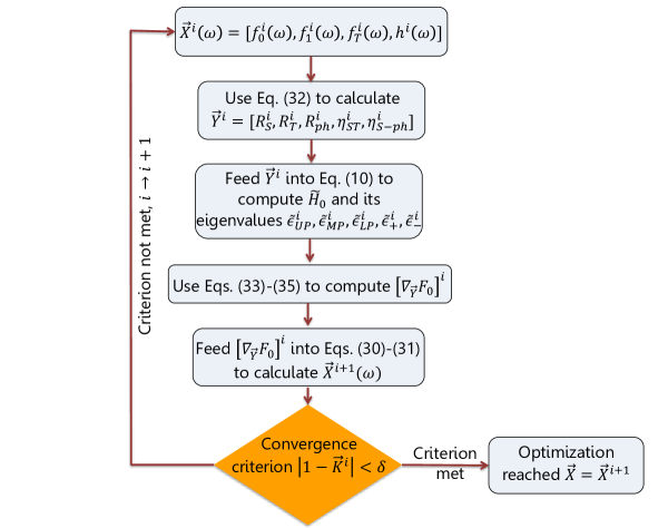
Figure 7: Flowchart that illustrates the self-consistent numerical optimization of $\vec{X}(\omega)=[f_{0}(\omega),f_{1}(\omega),f_{T}(\omega),h(\omega)]$. The $i$th iteration of the algorithm starts with $\vec{X}^{i}(\omega)=[f_{0}^{i}(\omega),f_{1}^{i}(\omega),f_{T}^{i}(\omega),h^{i}(\omega)]$ which at the beginning $(i=0)$, is chosen as the guess $\vec{X}^{0}(\omega)=[g_{S}(\omega),0,g_{T}(\omega),0]$ (corresponding to a full-polaron transformation ansatz). $\vec{X}^{i}(\omega)$ is subsequently used in Eq. (32) for the calculation of $\vec{Y}^{i}=[R_{S}^{i},R_{T}^{i},R_{ph}^{i},\eta_{ST}^{i},\eta_{S-ph}^{i}]$, which allows to build and numerically solve the renormalized Hamiltonian (10). The eigenvalues of the latter ($\tilde{\epsilon}_{UP}^{i}$,$\tilde{\epsilon}_{MP}^{i}$,$\tilde{\epsilon}_{LP}^{i}$,$\tilde{\epsilon}_{+}^{i},\tilde{\epsilon}_{-}^{i}$), in conjuction with Eqs. (33)–(35) to calculate $[\nabla_{\vec{Y}}F_{0}]^{i}$ which, via Eqs. (30)–(31), yield the guess $\vec{X}^{i+1}(\omega)$ to be used in the next iteration. This process is carried out until the convergence criterion is reached, which we define as $|\mathbf{1}-\vec{K}^{i}|<\delta$, where $\mathbf{1}=[1,1,1,1,1]$, $\vec{K}^{i}=\Bigg{[}\frac{R_{S}^{i+1}}{R_{S}^{i}},\frac{R_{T}^{i+1}}{R_{T}^{i}},\frac{R_{ph}^{i+1}}{R_{ph}^{i}},\frac{\eta_{ST}^{i+1}}{\eta_{ST}^{i}},\frac{\eta_{S-ph}^{i+1}}{\eta_{S-ph}^{i}}\Bigg{]}$, and $\delta=10^{-6}$.

Appendix B. Evaluation of rates

The rate of population transfer from eigenstate $m$ to $n$ of $\tilde{H}_{0}$ (see Eq. 10) is mediated by the residual interaction $\tilde{H}_{I}$ in Eq. (16), and can be calculated in terms of the corresponding autocorrelation function,

$$k_{m\rightarrow n} =\int_{-\infty}^{\infty}\langle\tilde{H}_{I}^{(m,n)}(\tau)\tilde{H}_{I}^{(m,n)}(0)^{*}\rangle d\tau$$

$$=\int_{-\infty}^{\infty}\big{\langle}\left[\tilde{V}_{ST}^{(m,n)}(\tau)+\tilde{V}_{S-ph}^{(m,n)}(\tau)+\tilde{V}_{S}^{(m,n)}(\tau)+\tilde{V}_{T}^{(m,n)}(\tau)+\tilde{V}_{ph}^{(m,n)}(\tau)\right]$$

$$\hskip 10.00002pt\times\left[\tilde{V}_{ST}^{(m,n)*}(0)+\tilde{V}_{S-ph}^{(m,n)*}(0)+\tilde{V}_{S}^{(m,n)*}(0)+\tilde{V}_{T}^{(m,n)*}(0)+\tilde{V}_{ph}^{(m,n)*}(0)\right]\big{\rangle}d\tau,$$ (36)

where $\tilde{V}_{x}^{(m,n)}(\tau)=\langle m|e^{i\tilde{H}_{S}\tau}\tilde{V}_{x}e^{-i\tilde{H}_{S}\tau}|n\rangle=e^{i(\omega_{m}-\omega_{n})\tau}\langle m|e^{iH_{B}\tau}\tilde{V}_{x}e^{-iH_{B}\tau}|n\rangle$ for $x=ST,\,S-ph,\,S,\,T,\,ph$.

From Eq. (36), we notice the emergence of auto- and cross-correlation terms which fall into one of three types, and are summarized in Table 2. Correlations of similar nature have been explored in previous works using a variational approach for energy transfer dynamics in chromophoric arrays McCutcheon and Nazir (2011); Pollock et al. (2013). In Table 2 we also show the specific forms of the correlation functions in time domain in the localized basis, upon which the rates in Eq. (36) can be calculated. Notice that we can further classify the correlations according to whether they emerge from averaging over the vibrational Hamiltonians of same or different electronic sites (see Table 2).

Summary of relevant correlation functions for dynamics calculations
Type: exponential-exponential
Same site	Different sites
$\begin{aligned} &\langle e^{\hat{D}_{ST}^{(n)}(\tau)}e^{\lambda\hat{D}_{ST}^{(n)}(0)}\rangle=\eta_{ST}^{2}\exp\big{[}Q(\lambda|\Delta_{ST}^{(0)}(\omega)|^{2}\\ &+\lambda(N-1)|f_{1}|^{2}(\omega),\tau)\big{]}\end{aligned}$	$\begin{aligned} &\langle e^{\hat{D}_{ST}^{(n)}(\tau)}e^{\lambda\hat{D}_{ST}^{(n)}(0)}\rangle=\eta_{ST}^{2}\exp\big{[}Q(\lambda|\Delta_{ST}^{(0)}(\omega)|^{2}\\ &+\lambda(N-1)|f_{1}|^{2}(\omega),\tau)\big{]}\end{aligned}$
$\begin{aligned} &\langle e^{\hat{D}_{S-ph}^{(n)}(\tau)}e^{\lambda\hat{D}_{S-ph}^{(n)}}\rangle=\eta_{S-ph}^{2}\exp\bigg{[}Q(\lambda|\Delta_{S-ph}^{(0)}(\omega)|^{2}\\ &+\lambda(N-1)|f_{1}(\omega)-h(\omega)|^{2},\tau)\bigg{]}\end{aligned}$	$\begin{aligned} &\langle e^{\hat{D}_{S-ph}^{(n)}(\tau)}e^{\lambda\hat{D}_{S-ph}^{(m)}}\rangle=\eta_{S-ph}^{2}\exp\bigg{[}Q(2\lambda\Delta_{S-ph}^{(0)}(\omega)\\ &\times(f_{1}(\omega)-h(\omega))+\lambda(N-2)|f_{1}(\omega)-h(\omega)|^{2},\tau)\bigg{]}\end{aligned}$
$\begin{aligned} &\langle e^{\hat{D}_{ST}^{(n)}(\tau)}e^{\lambda\hat{D}_{S-ph}^{(n)}(0)}\rangle=\eta_{ST}\eta_{S-ph}\exp\bigg{[}Q(\lambda|\Delta_{S-ph}^{(0)}(\omega)|^{2}+\\ &+\lambda(N-1)|f_{1}(\omega)-h(\omega)|^{2},\tau)\bigg{]}\end{aligned}$	$\begin{aligned} &\langle e^{\hat{D}_{ST}^{(n)}(\tau)}e^{\lambda\hat{D}_{S-ph}^{(m)}(0)}\rangle=\eta_{ST}\eta_{S-ph}\\ &\exp\bigg{\{}Q\bigg{[}\lambda\bigg{(}\Delta_{S-ph}^{(0)}(\omega)f_{1}(\omega)\\ &+(f_{1}(\omega)-h(\omega))\Delta_{ST}^{(0)}(\omega)\\ &+(N-2)f_{1}(\omega)(f_{1}(\omega)-h(\omega))\bigg{)},\tau\bigg{\}}\end{aligned}$
Type: exponential-linear
$\begin{aligned} &\langle e^{\lambda\hat{D}_{ST}^{(n)}(\tau)}\hat{D}_{S}^{(n)}(0)\rangle=\int_{0}^{\infty}d\omega\mathcal{D}(\omega)\lambda\big{[}\frac{(g_{S}(\omega)-f_{0}(\omega))\Delta_{ST}^{(0)}(\omega)}{\omega}+\\ &(N-1)\frac{|f_{1}(\omega)|^{2}}{\omega}\big{]}\times\left[\overline{n}(\omega)e^{i\omega\tau}-(\overline{n}(\omega)+1)e^{-i\omega\tau}\right]\eta_{ST}\end{aligned}$	$\begin{aligned} &\langle e^{\lambda\hat{D}_{ST}^{(n)}(\tau)}\hat{D}_{S}^{(m)}(0)\rangle=\int_{0}^{\infty}d\omega\mathcal{D}(\omega)\lambda\bigg{[}(g_{S}(\omega)-f_{0}(\omega)\\ &-(N-2)f_{1}(\omega))\frac{f_{1}(\omega)}{\omega}-f_{1}(\omega)\frac{\Delta_{ST}^{(0)}(\omega)}{\omega}\bigg{]}\\ &\times\left[\overline{n}(\omega)e^{i\omega\tau}-(\overline{n}(\omega)+1)e^{-i\omega\tau}\right]\eta_{ST}\end{aligned}$
$\begin{aligned} &\langle e^{\lambda\hat{D}_{ST}^{(n)}(\tau)}\hat{D}_{T}^{(n)}(0)\rangle=\int_{0}^{\infty}d\omega\mathcal{D}(\omega)\lambda\frac{(g_{T}(\omega)-f_{T}(\omega))\Delta_{ST}^{(0)}(\omega)}{\omega}\\ &\times\left[\overline{n}(\omega)e^{i\omega\tau}-(\overline{n}(\omega)+1)e^{-i\omega\tau}\right]\eta_{ST}d\omega\end{aligned}$	$\begin{aligned} &\langle e^{\lambda\hat{D}_{ST}^{(n)}(\tau)}\hat{D}_{T}^{(m)}(0)\rangle=\int_{0}^{\infty}d\omega\mathcal{D}(\omega)\lambda\frac{(g_{T}(\omega)-f_{T}(\omega))f_{1}(\omega)}{\omega}\\ &\times\left[\overline{n}(\omega)e^{i\omega\tau}-(\overline{n}(\omega)+1)e^{-i\omega\tau}\right]\eta_{ST}\end{aligned}$
$\begin{aligned} &\langle e^{\lambda\hat{D}_{S-ph}^{(n)}(\tau)}\hat{D}_{S}^{(n)}(0)\rangle=\int_{0}^{\infty}d\omega\mathcal{D}(\omega)\lambda\bigg{[}\frac{(g_{S}(\omega)-f_{0}(\omega))\Delta_{S-ph}^{(0)}(\omega)}{\omega}\\ &-(N-1)\frac{f_{1}(\omega)\Delta_{S-ph}^{(1)}(\omega)}{\omega}\bigg{]}\\ &\times\left[\overline{n}(\omega)e^{i\omega\tau}-(\overline{n}(\omega)+1)e^{-i\omega\tau}\right]\eta_{S-ph}\end{aligned}$	$\begin{aligned} &\langle e^{\lambda\hat{D}_{S-ph}^{(n)}(\tau)}\hat{D}_{S}^{(m)}(0)\rangle=\int_{0}^{\infty}d\omega\mathcal{D}(\omega)\lambda\bigg{[}2\frac{(g_{S}(\omega)-f_{0}(\omega))}{\omega}\\ &\times\Delta_{S-ph}^{(1)}(\omega)-(N-2)\frac{f_{1}(\omega)\Delta_{S-ph}^{(1)}(\omega)}{\omega}\bigg{]}\\ &\times\left[\overline{n}(\omega)e^{i\omega\tau}-(\overline{n}(\omega)+1)e^{-i\omega\tau}\right]\eta_{S-ph}\end{aligned}$
Type: linear-linear
$\begin{aligned} &\langle\hat{D}_{S}^{(n)}(\tau)\hat{D}_{S}^{(n)}(0)\rangle=\int_{0}^{\infty}d\omega\mathcal{D}(\omega)\big{[}|g_{S}(\omega)-f_{0}(\omega)|^{2}+|f_{1}(\omega)|^{2}(N-1)\big{]}\\ &\times\big{[}\overline{n}(\omega)e^{i\omega\tau}+(\overline{n}(\omega)+1)e^{-i\omega\tau}\big{]}\end{aligned}$	$\begin{aligned} &\langle\hat{D}_{S}^{(n)}(\tau)\hat{D}_{S}^{(m)}(0)\rangle=\int_{0}^{\infty}d\omega\mathcal{D}(\omega)\big{[}-2(g_{S}(\omega)-f_{0}(\omega))f_{1}(\omega)\\ &+(N-2)|f_{1}(\omega)|^{2}\big{]}\times\big{[}\overline{n}(\omega)e^{i\omega\tau}+(\overline{n}(\omega)+1)e^{-i\omega\tau}\big{]}\end{aligned}$
$\begin{aligned} &\langle\hat{D}_{S}^{(n)}(\tau)\hat{D}_{T}^{(n)}(0)\rangle=\int_{0}^{\infty}d\omega\mathcal{D}(\omega)(g_{S}(\omega)-f_{0}(\omega))(g_{T}(\omega)-f_{T}(\omega))\\ &\times\big{[}\overline{n}(\omega)e^{i\omega\tau}+(\overline{n}(\omega)+1)e^{-i\omega\tau}\big{]}\end{aligned}$	$\begin{aligned} \langle\hat{D}_{S}^{(n)}(\tau)\hat{D}_{T}^{(m)}(0)\rangle&=-\int_{0}^{\infty}d\omega\mathcal{D}(\omega)f_{1}(\omega)(g_{T}(\omega)-f_{T}(\omega))\\ &\times\big{[}\overline{n}(\omega)e^{i\omega\tau}+(\overline{n}(\omega)+1)e^{-i\omega\tau}\big{]}\end{aligned}$
$\begin{aligned} &\langle\hat{D}_{T}^{(n)}(\tau)\hat{D}_{T}^{(n)}(0)\rangle=\int_{0}^{\infty}d\omega\mathcal{D}(\omega)|g_{T}(\omega)-f_{T}(\omega)|^{2}\\ &\times\big{[}\overline{n}(\omega)e^{i\omega\tau}+(\overline{n}(\omega)+1)e^{-i\omega\tau}\big{]}\end{aligned}$

Table 2: Relevant correlation functions. For simplicity in the notation, we introduce $Q(A(\omega),\tau)=\int_{0}^{\infty}d\omega\mathcal{D}(\omega)\frac{A(\omega)}{\omega^{2}}\left[i\sin(\omega\tau)-\cos(\omega\tau)\coth(\beta\omega/2)\right]$, $\Delta_{ST}^{(i)}=f_{i}(\omega)-f_{T}(\omega)$, and $\Delta_{S-ph}^{(i)}=f_{i}(\omega)-h(\omega)$ where, as defined above, $\mathcal{D}(\omega)$ is the vibrational DOS. We also introduce the scaling factor $\lambda=\pm 1$.

Once the time-domain correlation functions are calculated, we Fourier transform them to obtain the rates of population transfer between the chemical species of interest in our model. Given the variationally optimized $\vec{X}(\omega)$, these rates can be analytically calculated for the linear-linear and linear-exponential type correlations, by using relations of the form

$$\int_{-\infty}^{\infty}\langle\hat{D}_{S}^{(n)}(\tau)\hat{D}_{S}^{(n)}(0)\rangle e^{i\omega_{0}\tau}d\tau =\big{[}(g_{S}(-\omega_{0})-f_{0}(-\omega_{0}))^{2}+|f_{1}(-\omega_{0})|^{2}(N-1)\big{]}\overline{n}(-\omega_{0})\Theta(-\omega_{0})$$

$$\hskip 10.00002pt+\big{[}(g_{S}(\omega_{0})-f_{0}(\omega_{0}))^{2}+|f_{1}(\omega_{0})|^{2}(N-1)\big{]}\big{[}\overline{n}(\omega_{0})+1\big{]}\Theta(\omega_{0}),$$ (37)

where $\bar{n}(\omega)=(e^{\beta\omega}-1)^{-1}$ is the boson occupation number and $\Theta(\omega)=1$ if $\omega>0$ and 0 otherwise. Eq. (37) can be readily understood as a Fermi golden rule population transfer rate due to a single phonon absorption (first row) or emission process (second row); expressions like this also arise in standard Redfield theory Nitzan (2006).

On the other hand, the Fourier transform of the exponential-exponential type correlation function is of the form $I=\int_{-\infty}^{\infty}e^{Q(A(\omega),\tau)}e^{i\omega_{0}\tau}d\tau$. This integral can be approximated by means of the steepest descent method Weiss (2012), which consists on the analytical continuation of $Q(A(\omega),\tau)\rightarrow Q(A(\omega),z=\tau_{R}+i\tau_{I})$ (see Table 2),

$$Q(A(\omega),z) =-\int_{0}^{\infty}d\omega\mathcal{D}(\omega)\frac{A(\omega)}{\omega^{2}}\left[\coth(\beta\omega/2)\cos(\omega\tau_{R})\cosh(\omega\tau_{I})+\cos(\omega\tau_{R})\sinh(\omega\tau_{I})\right]$$

$$\hskip 10.00002pt+i\int_{0}^{\infty}d\omega\mathcal{D}(\omega)\frac{A(\omega)}{\omega^{2}}\left[\coth(\beta\omega/2)\sin(\omega\tau_{R})\sinh(\omega\tau_{I})+\sin(\omega\tau_{R})\cosh(\omega\tau_{I})\right].$$ (38)

Let us rewrite $I=\int_{-\infty}^{\infty}e^{R(A(\omega),\tau)}d\tau$, where $R(A(\omega),z)=Q(A(\omega),z)+i\omega_{0}z$, and find the saddle point $z^{*}$ around which we will approximate the integral,

$$\frac{dR(A(\omega),z^{*})}{dz}=\frac{\partial R(A(\omega),z^{*})}{i\partial\tau_{I}}=\frac{\partial\Im Q(A(\omega),z^{*})}{\partial\tau_{I}}+i\Bigg{(}\omega_{0}-\frac{\partial\Re Q(A(\omega),z^{*})}{\partial\tau_{I}}\Bigg{)}=0.$$ (39)

In Eq. (39), we took advantage of the analyticity of $R(A(\omega),z)$, which guarantees the derivative being independent of the direction of differentiation in the complex plane. From Eqs. (38) and (39), we have that $\tau_{R}=0$. Therefore, we obtain

$$\frac{dR(A(\omega),z^{*})}{dz} =\int_{0}^{\infty}d\omega\mathcal{D}(\omega)\frac{A(\omega)}{\omega}\big{[}\coth(\beta\omega/2)\sinh(\omega\tau_{I}^{*})$$ (40)

$$+\cosh(\omega\tau_{I}^{*})\big{]}+\omega_{0}=0,$$

where we notice that for $\omega_{0}=0$, the saddle point is at $\tau_{I}^{*}=-\frac{\beta}{2}$. For $\omega_{0}\neq 0$, we rely on the numerical solution of Eq. (40) to find the root $z^{*}=i\tau_{I}^{*}$ such that

$$\int_{-\infty}^{\infty}e^{Q(A(\omega),z)}e^{i\omega_{0}z}dz\approx\left(\frac{1}{2\pi R^{\prime\prime}(A(\omega),z^{*})}\right)^{1/2}e^{R(A(\omega),\tau_{I}^{*})},$$ (41)

where the prime denotes differentiation with respect to $\tau_{I}^{*}$, and

$$R^{\prime\prime}(A(\omega),z^{*}) =\int_{0}^{\infty}d\omega\mathcal{D}(\omega)A(\omega)\big{[}\coth(\beta\omega/2)\cosh(\omega\tau_{I}^{*})$$ (42)

$$+\sinh(\omega\tau_{I}^{*})\big{]}.$$

Eq. (41) is a generalization of the classical Marcus rate, where $e^{R(A(\omega),\tau_{I}^{*})}$ is a Boltzmann factor corresponding to an effective activation energy, and $\left(\frac{1}{2\pi R^{\prime\prime}(A(\omega),z^{*})}\right)^{1/2}$ is a density of states prefactor.

VII Acknowledgments

L.A.M.M is grateful for support of a UC-Mexus CONACyT scholarship for doctoral studies. L.A.M.M. and J.Y.Z. acknowledge support of NSF EAGER CHE-1836599. S.K.C. acknowledges support from the Canada Research Chairs program and NSERC RGPIN-2014-06129. L.A.M.M. acknowledges Raphael F. Ribeiro, Jorge Campos-González-Angulo, and Matthew Du for useful discussions.

References

• Törmä and Barnes (2014) P. Törmä and W. L. Barnes, Rep. Prog. Phys. 78, 013901 (2014).
• Ebbesen (2016) T. W. Ebbesen, Acc. Chem. Res. 49, 2403 (2016).
• Ribeiro et al. (2018) R. F. Ribeiro, L. A. Martínez-Martínez, M. Du, J. Campos-Gonzalez-Angulo,  and J. Yuen-Zhou, Chem. Sci. 9, 6325 (2018).
• Feist et al. (2018) J. Feist, J. Galego,  and F. J. Garcia-Vidal, ACS Photonics 5, 205 (2018).
• Flick et al. (2018) J. Flick, N. Rivera,  and P. Narang, Nanophotonics 7, 1479 (2018).
• Hopfield (1958) J. J. Hopfield, Phys. Rev. 112, 1555 (1958).
• Hutchison et al. (2012) J. A. Hutchison, T. Schwartz, C. Genet, E. Devaux,  and T. W. Ebbesen, Angew. Chem. Int. Ed. 51, 1592 (2012).
• Zhong et al. (2016) X. Zhong, T. Chervy, S. Wang, J. George, A. Thomas, J. A. Hutchison, E. Devaux, C. Genet,  and T. W. Ebbesen, Angew. Chem. Int. Ed. 55, 6202 (2016).
• Du et al. (2018) M. Du, R. F. Ribeiro,  and J. Yuen-Zhou, arXiv preprint arXiv:1810.10083  (2018).
• Sáez-Blázquez et al. (2018) R. Sáez-Blázquez, J. Feist, A. I. Fernández-Domínguez,  and F. J. García-Vidal, Phys. Rev. B 97, 241407 (2018).
• Neuman et al. (2018) T. Neuman, R. Esteban, D. Casanova, F. J. García-Vidal,  and J. Aizpurua, Nano Lett. 18, 2358 (2018).
• Feist and Garcia-Vidal (2015) J. Feist and F. J. Garcia-Vidal, Phys. Rev. Lett. 114, 196402 (2015).
• Schachenmayer et al. (2015) J. Schachenmayer, C. Genes, E. Tignone,  and G. Pupillo, Phys. Rev. Lett. 114, 196403 (2015).
• Kéna-Cohen and Forrest (2007) S. Kéna-Cohen and S. R. Forrest, Phys. Rev. B 76, 075202 (2007).
• Stranius et al. (2018) K. Stranius, M. Hertzog,  and K. Börjesson, Nat. Commun. 9, 2273 (2018).
• Polak et al. (2018) D. Polak, R. Jayaprakash, A. Leventis, K. J. Fallon, H. Coulthard, I. Petty, J. Anthony, J. Anthony, H. Bronstein, D. G. Lidzey, et al., arXiv preprint arXiv:1806.09990  (2018).
• Thomas et al. (2016) A. Thomas, J. George, A. Shalabney, M. Dryzhakov, S. J. Varma, J. Moran, T. Chervy, X. Zhong, E. Devaux, C. Genet, et al., Angew. Chem. Int. Ed. 55, 11462 (2016).
• Dunkelberger et al. (2016) A. Dunkelberger, B. Spann, K. Fears, B. Simpkins,  and J. Owrutsky, Nat. Commun. 7, 13504 (2016).
• Chervy et al. (2017) T. Chervy, A. Thomas, E. Akiki, R. M. Vergauwe, A. Shalabney, J. George, E. Devaux, J. A. Hutchison, C. Genet,  and T. W. Ebbesen, ACS Photonics 5, 217 (2017).
• F. Ribeiro et al. (2018) R. F. Ribeiro, A. D. Dunkelberger, B. Xiang, W. Xiong, B. S. Simpkins, J. C. Owrutsky,  and J. Yuen-Zhou, J. Phys. Chem. Lett. 9, 3766 (2018).
• Xiang et al. (2018) B. Xiang, R. F. Ribeiro, A. D. Dunkelberger, J. Wang, Y. Li, B. S. Simpkins, J. C. Owrutsky, J. Yuen-Zhou,  and W. Xiong, Proc. Natl. Acad. Sci. U.S.A. 115, 4845 (2018).
• Bajoni et al. (2008) D. Bajoni, E. Semenova, A. Lemaître, S. Bouchoule, E. Wertz, P. Senellart,  and J. Bloch, Phys. Rev. B 77, 113303 (2008).
• Eizner et al. (2018) E. Eizner, J. Brodeur, F. Barachati, A. Sridharan,  and S. Kéna-Cohen, ACS Photonics 5, 2921 (2018).
• Chakraborty et al. (2018) B. Chakraborty, J. Gu, Z. Sun, M. Khatoniar, R. Bushati, A. L. Boehmke, R. Koots,  and V. M. Menon, Nano Lett. 18, 6455 (2018).
• Gubbin et al. (2014) C. R. Gubbin, S. A. Maier,  and S. Kéna-Cohen, Appl. Phys. Lett. 104, 233302 (2014).
• Mazzeo et al. (2014) M. Mazzeo, A. Genco, S. Gambino, D. Ballarini, F. Mangione, O. Di Stefano, S. Patanè, S. Savasta, D. Sanvitto,  and G. Gigli, Appl. Phys. Lett. 104, 233303 (2014).
• Genco et al. (2018) A. Genco, A. Ridolfo, S. Savasta, S. Patané, G. Gigli,  and M. Mazzeo, Adv. Opt. Mat. 6, 1800364 (2018).
• Eizner et al. (2019) E. Eizner, L. A. Martínez-Martínez, J. Yuen-Zhou,  and S. Kéna-Cohen, arXiv preprint arXiv:1903.09251  (2019).
• del Pino et al. (2015) J. del Pino, J. Feist,  and F. J. Garcia-Vidal, New J. Phys. 17, 053040 (2015).
• Galego et al. (2016) J. Galego, F. J. Garcia-Vidal,  and J. Feist, Nat. Commun. 7, 13841 (2016).
• Herrera and Spano (2016) F. Herrera and F. C. Spano, Phys. Rev. Lett. 116, 238301 (2016)arXiv:1512.05017 .
• Herrera and Spano (2017) F. Herrera and F. C. Spano, Phys. Rev. Lett. 118, 223601 (2017).
• Galego et al. (2017) J. Galego, F. J. Garcia-Vidal,  and J. Feist, Phys. Rev. Lett. 119, 136001 (2017).
• Martínez-Martínez et al. (2018) L. A. Martínez-Martínez, M. Du, R. F. Ribeiro, S. Kéna-Cohen,  and J. Yuen-Zhou, J. Phy. Chem. Lett. 9, 1951 (2018).
• Tischler et al. (2005) J. R. Tischler, M. S. Bradley, V. Bulović, J. H. Song,  and A. Nurmikko, Phys. Rev. Lett. 95, 036401 (2005).
• Silbey (1984) R. Silbey, J. Chem. Phys. 80, 2615 (1984).
• Harris and Silbey (1985) R. A. Harris and R. Silbey, J. Chem. Phys 83, 1069 (1985).
• Pollock et al. (2013) F. A. Pollock, D. P. McCutcheon, B. W. Lovett, E. M. Gauger,  and A. Nazir, New J. Phys. 15, 075018 (2013).
• Wu et al. (2016) N. Wu, J. Feist,  and F. J. Garcia-Vidal, Phys. Rev. B 94, 195409 (2016).
• Daskalakis et al. (2017) K. S. Daskalakis, S. A. Maier,  and S. Kéna-Cohen, in Quantum Plasmonics (Springer, 2017) pp. 151–163.
• Lee et al. (2012) C. K. Lee, J. Moix,  and J. Cao, J. Chem. Phys 136, 204120 (2012).
• Makri and Makarov (1995a) N. Makri and D. E. Makarov, J. Chem. Phys 102, 4600 (1995a).
• Makri and Makarov (1995b) N. Makri and D. E. Makarov, J. Chem. Phys 102, 4611 (1995b).
• Meyer et al. (1990) H.-D. Meyer, U. Manthe,  and L. S. Cederbaum, Chem. Phys. Lett. 165, 73 (1990).
• Beck et al. (2000) M. H. Beck, A. Jäckle, G. Worth,  and H.-D. Meyer, Phys. Rep. 324, 1 (2000).
• Ishizaki and Fleming (2009) A. Ishizaki and G. R. Fleming, J. Chem. Phys. 130, 234111 (2009).
• Huo and Coker (2011) P. Huo and D. F. Coker, J. Chem. Phys. 135, 201101 (2011).
• Tully (1990) J. C. Tully, J. Chem. Phys. 93, 1061 (1990).
• Prezhdo and Rossky (1997) O. V. Prezhdo and P. J. Rossky, J. Chem. Phys. 107, 825 (1997).
• Subotnik et al. (2016) J. E. Subotnik, A. Jain, B. Landry, A. Petit, W. Ouyang,  and N. Bellonzi, Annu. Rev. Phys. Chem. 67, 387 (2016).
• Hoffmann et al. (2018) N. M. Hoffmann, H. Appel, A. Rubio,  and N. T. Maitra, Eur. Phys. J. B 91, 180 (2018).
• Zeb et al. (2018) M. A. Zeb, P. G. Kirton,  and J. Keeling, ACS Photonics 5, 249 (2018).
• Agranovich et al. (2003) V. M. Agranovich, M. Litinskaya,  and D. G. Lidzey, Phys. Rev. B 67, 085311 (2003).
• Litinskaya et al. (2004) M. Litinskaya, P. Reineker,  and V. M. Agranovich, J. Lumin. 110, 364 (2004).
• Rebentrost et al. (2009) P. Rebentrost, M. Mohseni,  and A. Aspuru-Guzik, J. Phys. Chem. B 113, 9942 (2009).
• Chen et al. (2015) X.-K. Chen, S.-F. Zhang, J.-X. Fan,  and A.-M. Ren, J. Phys. Chem. C 119, 9728 (2015).
• Yang et al. (2017) Z. Yang, Z. Mao, Z. Xie, Y. Zhang, S. Liu, J. Zhao, J. Xu, Z. Chi,  and M. P. Aldred, Chem. Soc. Rev. 46, 915 (2017).
• Peng et al. (2017) Q. Peng, D. Fan, R. Duan, Y. Yi, Y. Niu, D. Wang,  and Z. Shuai, J. Phys. Chem. C 121, 13448 (2017).
• Yost et al. (2014) S. R. Yost, J. Lee, M. W. Wilson, T. Wu, D. P. McMahon, R. R. Parkhurst, N. J. Thompson, D. N. Congreve, A. Rao, K. Johnson, et al., Nat. Chem. 6, 492 (2014).
• Herrera and Spano (2018) F. Herrera and F. C. Spano, ACS Photonics 5, 65 (2018).
• Fofang et al. (2011) N. T. Fofang, N. K. Grady, Z. Fan, A. O. Govorov,  and N. J. Halas, Nano Lett. 11, 1556 (2011).
• Bisht et al. (2018) A. Bisht, J. Cuadra, M. Wersäll, A. Canales, T. J. Antosiewicz,  and T. Shegai, Nano Lett. 19, 189 (2018).
• Campos-Gonzalez-Angulo et al. (2019) J. Campos-Gonzalez-Angulo, R. F. Ribeiro,  and J. Yuen-Zhou, arXiv preprint arXiv:1902.10264  (2019).
• Munkhbat et al. (2018) B. Munkhbat, M. Wersäll, D. G. Baranov, T. J. Antosiewicz,  and T. Shegai, Sci. Adv. 4, eaas9552 (2018).
• Semenov and Nitzan (2019) A. Semenov and A. Nitzan, arXiv preprint arXiv:1902.08896  (2019).
• McCutcheon and Nazir (2011) D. P. McCutcheon and A. Nazir, J. Chem. Phys. 135, 114501 (2011).
• Nitzan (2006) A. Nitzan, Chemical dynamics in condensed phases: relaxation, transfer and reactions in condensed molecular systems (Oxford university press, 2006).
• Weiss (2012) U. Weiss, Quantum dissipative systems, Vol. 13 (World scientific, 2012).