Role of magnetic field curvature in magnetohydrodynamic turbulence

Abstract

Magnetic field are transported and tangled by turbulence, even as they lose identity due to nonideal or resistive effects. On balance field lines undergo stretch-twist-fold processes. The curvature field, a scalar that measures the tangling of the magnetic field lines, is studied in detail here, in the context of magnetohydrodynamic turbulence. A central finding is that the magnitudes of the curvature and the magnetic field are anti-correlated. High curvature co-locates with low magnetic field, which gives rise to power-law tails of the probability density function of the curvature field. The curvature drift term that converts magnetic energy into flow and thermal energy, largely depends on the curvature field behavior, a relationship that helps to explain particle acceleration due to curvature drift. This adds as well to evidence that turbulent effects most likely play an essential role in particle energization since turbulence drives stronger tangled field configurations, and therefore curvature.

I Introduction

A divergence-free vector field, such as the magnetic field, can be conveniently visualized in terms of field lines, which are tangent to the field everywhere. In many astrophysical and space plasmas, magnetic field lines play an essential role, in general for describing topology and connectivity at a single instant of time, and even for developing theoretical descriptions of dynamical processes such as magnetic reconnection Parker (1979). Magnetic field lines are also widely used in describing mechanisms for particle acceleration and for the transport of suprathermal and energetic particles. Ambiguities in defining field lines, especially as a function of time, are well known Newcomb (1958). In turbulence, magnetic field lines are in geneal not well-ordered, but rather exhibit complex structures and wander randomly in space Jokipii (1966); Jokipii and Parker (1969); Matthaeus et al. (1995). Moving into the realm of magnetic reconnection, the field lines can “disconnect” and “reconnect”. Given these ambiguities inherent in the magnetic field line formalism, here we avoid committing to a focus on the trajectory of the magnetic field integral curves, and instead prefer to consider an intrinsic geometric parameter: curvature, that completely determines a curve in 2D space.

The curvature $\kappa$, measuring how rapidly a curve changes direction in space, is defined as

$$\kappa=\left\|\boldsymbol{b}\cdot\nabla\boldsymbol{b}\right\|.$$ (1)

where $\boldsymbol{b}=\boldsymbol{B}/\left\|\boldsymbol{B}\right\|$. The curvature of magnetic field lines is related directly to the curvature drift of the motion of charged particles, which is invoked in certain particle acceleration mechanisms, e.g., first-order Fermi mechanism in magnetic reconnection Northrop (1961); Drake et al. (2006). Indeed, rapid advances in computations and observations have improved understanding of several features of magnetic reconnection Hoshino et al. (2001); Egedal, Daughton, and Le (2012); Drake et al. (2006); Oka et al. (2010); Pritchett (2006) that might contribute to particle energization. For example, the curvature drift mechanism (related to the first-order Fermi mechanism) has been identified as the dominant source of electron heating with a weak guide field Dahlin, Drake, and Swisdak (2014, 2017); Li et al. (2017, 2015); Guo et al. (2014); Lu et al. (2018); Wang et al. (2016, 2017). One might reason in a qualitative sense: we think of bent field lines as elastic bands under tension, exerting a force ($\sim\kappa B^{2}$) on the fluid. This force will drive flows as the lines straighten out. It is natural then to inquire the extent to which the curvature drift acceleration and the curvature field are spatially and quantitatively correlated.

Although there is hardly any doubt that the curvature, as a essential feature of the geometrical behavior of magnetic field lines, is a key ingredient in certain particle acceleration mechanisms, the detailed properties of the magnetic field curvature is neither well known nor well understood for general configuration. The study presented in this letter addresses this problem by employing numerical simulations of magnetohydrodynamic (MHD) turbulence, with the goal of providing better physical interpretation of curvature drift acceleration. We find that intense curvature and small magnetic field are preferentially colocated. Intense curvature tends to be linearly anti-correlated with the square of magnetic magnitude. Therefore, magnetic energy release via the curvature drift term is in strong association with the curvature field. This result provides new insights into the literature on particle energization during magnetic reconnection, and also favors the influence of turbulent magnetic effects on heating.

II Method

We consider two-dimensional incompressible MHD turbulence. The dynamical equations read

$${\frac{\partial\omega}{\partial t}}+\left(\boldsymbol{v}\cdot\nabla\right)\omega = \left(\boldsymbol{B}\cdot\nabla\right)j+\nu\nabla^{2}\omega,$$ (2)

$${\frac{\partial a}{\partial t}}+\left(\boldsymbol{v}\cdot\nabla\right)a = \eta\nabla^{2}a,$$ (3)

where $\boldsymbol{v}$ is the velocity field, $\omega=(\nabla\times\boldsymbol{v})\cdot\hat{\boldsymbol{z}}$ is the vorticity, $a$ is the magnetic potential, $\boldsymbol{B}=\nabla a\times\hat{\boldsymbol{z}}$ is the magnetic field, and $j=(\nabla\times\boldsymbol{B})\cdot\hat{\boldsymbol{z}}=-\nabla^{2}a$ is the electric current density. For simplicity, the viscosity $\nu$ and resistivity $\eta$ are set to equal values. The numerical simulation is done with a Fourier spectral method Wan et al. (2013) in a doubly periodic $(2\pi)^{2}$ cartesian domain with a $8192^{2}$ resolution. The fields are initialized at modes $5\leq|\boldsymbol{k}|\leq 20$ with random phases and fluctuation amplitudes, whose spectra are proportional to $1/\left[1+(k/k_{0})^{8/3}\right]$ with $k_{0}=10$. The total kinetic and magnetic energy are each initially equal to $0.5$. We fix $\nu=\eta=5\times 10^{-5}$, which corresponds to high Reynolds number. We carry out our analysis on snapshots near the time of maximum mean square electric current density.

III Anti-correlation between curvature and magnetic field

Curvature is a well-studied geometric characteristic of particle trajectories, its statistical properties having been reported in numerous hydrodynamic turbulence studies Braun, De Lillo, and Eckhardt (2006); Xu, Ouellette, and Bodenschatz (2007); Ouellette and Gollub (2007, 2008); Scagliarini (2011); Kadoch et al. (2011); Yang et al. (2013). Particle trajectories are manifestly different from magnetic field lines, but similar analysis methods are useful to study both cases. As a first step we compute the probability distribution function (PDF) of field line curvature in the above-described MHD simulation. The results, shown in Fig. 1, reveal properties that are surprisingly reminiscent of the hydrodynamic particle trajectory case. The distribution is broad and exhibits two clear power-law regimes – a low-curvature plateau scaling as $\sim\kappa^{0}$, while, the distribution of large curvatures scales as $\sim\kappa^{-2}$.

The physical origins of this feature become more apparent when we rewrite the Lorentz force in terms of $\boldsymbol{B}$, $\boldsymbol{j}\times\boldsymbol{B}=\boldsymbol{B}\cdot\nabla\boldsymbol{B}-\nabla\left(\boldsymbol{B}^{2}/2\right)$, where the second term acts in the same way as the pressure force and the first term is equivalent to $\nabla\cdot\left(\boldsymbol{B}\boldsymbol{B}\right)$, which can be interpreted as the effect of the surface stress $B_{i}B_{j}$ on fluids. Then we rewrite the force $\boldsymbol{B}\cdot\nabla\boldsymbol{B}$ in terms of curvilinear coordinates attached to a field line,

$$\boldsymbol{B}\cdot\nabla\boldsymbol{B}=B{\dfrac{\partial B}{\partial s}}\boldsymbol{t}-{\dfrac{B^{2}}{R}}\boldsymbol{n}.$$ (4)

Here $B=\left\|\boldsymbol{B}\right\|$, $s$ is a coordinate along the field line, $\boldsymbol{t}=\boldsymbol{b}$ and $\boldsymbol{n}$ are unit vectors in the tangential and normal directions, respectively, and $R=1/\kappa$ is the local field line radius. It follows that the curvature can be expressed as

$$\kappa=\frac{\left\|\boldsymbol{b}\times\left(\boldsymbol{B}\cdot\nabla\boldsymbol{B}\right)\right\|}{B^{2}}=\frac{f_{n}}{B^{2}}.$$ (5)

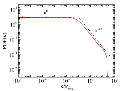
Figure 1: PDF of the magnetic field curvature $\kappa$ normalized to the root mean square value $\kappa_{\rm rms}$. The PDF has a $\kappa^{0}$ low-curvature regime and a $\kappa^{-2}$ high-curvature tail.

According to Eq. 5, one might expect that large normal force $f_{n}$ and small magnetic field both correspond to high curvature. However, from the joint PDFs in Fig. 2, one can see that high curvature is not strongly correlated with large normal force but instead is well associated with small magnetic field magnitude, while their effects are opposite for low curvature. By locating the small and large values of the curvature field, values $\kappa/\kappa_{\rm rms}<0.01$ and $\kappa/\kappa_{\rm rms}>0.2$ are plotted on the top of the color map of magnetic magnitude in Fig. 3, which correspond to the $\kappa^{0}$ low-curvature and $\kappa^{-2}$ high-curvature tails shown in Fig. 1, respectively. No qualitative associations between low curvature and large magnetic magnitude have been observed in Fig. 3(a), while we can readily identify the concentration of high curvature in regions of low magnetic magnitude in Fig. 3(b). These regions of low magnetic field strength are organized into twisted lines and isolated points. The solitary points are visually found in the vicinity of magnetic island cores, where the direction of magnetic field changes significantly, leading to high curvature. The high-curvature lines are preferentially in the form of sheet-like structures around the rims of islands, reminiscent of the well-studied configuration of sheets of electric current density. It is likely, of course, that this association is also related to potential sites of magnetic reconnection Parker (1979).

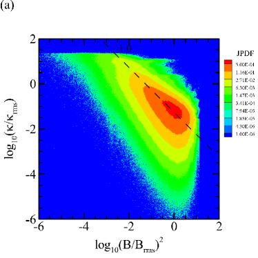
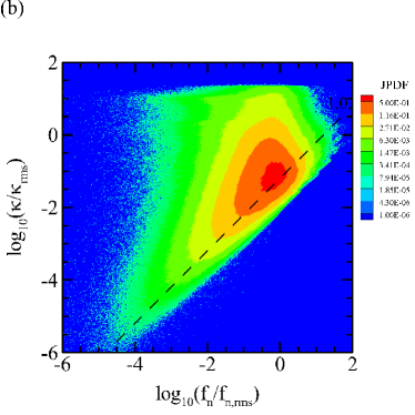
Figure 2: Joint PDFs of the curvature $\kappa$ and (a) the square of magnetic magnitude $B^{2}$ and (b) the force magnitude $f_{n}$ acting normal to field lines. All quantities are normalized to their respective root mean square values. There are apparent associations between high curvature and low magnetic field and between low curvature and low normal force.

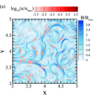
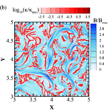
Figure 3: Contour maps of curvature superposed on color map of magnetic magnitude in a subregion of the whole domain. (a) Only $\kappa/\kappa_{\rm rms}<0.01$ values are pictured; (b) Only $\kappa/\kappa_{\rm rms}>0.2$ values are pictured. High curvature populates in regions of low magnetic field.

Based on the above results, we expect that the large-curvature (i.e. $\kappa\rightarrow\infty$) and small-curvature (i.e. $\kappa\rightarrow 0$) regimes in Fig. 1 should be determined by the scaling behavior of $1/B^{2}$ as $B\rightarrow 0$ and $f_{n}$ as $f_{n}\rightarrow 0$, respectively. To make these connections, one may begin by recalling that the $x$ and $y$ components of magnetic fluctuations are independent in isotropic MHD turbulence, and have quasi-Gaussian distributions. The square of magnetic magnitude $B^{2}=B_{x}^{2}+B_{y}^{2}$ therefore follows a chi-squared distribution with 2 degrees of freedom, deriving the $\kappa^{-2}$ high-curvature tail as $B\rightarrow 0$ by using Taylor expansion. Continuing, suppose we assume that the force $f_{n}$ at low values is a quasi-Gaussian random variable, recognizing that it could deviate from Gaussian distribution at high values due to intermittency. Then the $\kappa^{0}$ low-curvature tail is recovered as $f_{n}\rightarrow 0$.

IV Curvature drift acceleration

The discovery of the anti-correlation between curvature and magnetic fields is particularly suggestive of some generalizable physical process, such as curvature drift acceleration. From the Faraday’s law, one readily finds the equation governing magnetic energy $E^{m}=B^{2}/2$,

$$\frac{\partial E^{m}}{\partial t}+\nabla\cdot\left(\boldsymbol{E}\times\boldsymbol{B}\right)=-\boldsymbol{E}\cdot\boldsymbol{j},$$ (6)

wherein $\boldsymbol{E}\cdot\boldsymbol{j}=\boldsymbol{E}\cdot\boldsymbol{j}_{\parallel}+\boldsymbol{E}\cdot\boldsymbol{j}_{\perp}$, and $(\cdots)_{\parallel}$ and $(\cdots)_{\perp}$ are quantities parallel and perpendicular with respect to the local magnetic field direction. The perpendicular one can be further decomposed as $\boldsymbol{E}\cdot\boldsymbol{j}_{\perp}=\boldsymbol{E}\cdot\left[\dfrac{\boldsymbol{B}\times\left(\boldsymbol{B}\cdot\nabla\right)\boldsymbol{B}}{B^{2}}\right]-\nabla\left(\dfrac{B^{2}}{2}\right)\cdot{\dfrac{\boldsymbol{E}\times\boldsymbol{B}}{B^{2}}}$, where the second term on the right-hand side can be combined with the second term on the left-hand side in Eq. 6. The remaining term due to curvature drift is

$$\boldsymbol{E}\cdot\boldsymbol{j}_{c}=\boldsymbol{E}\cdot\left[\frac{\boldsymbol{B}\times\left(\boldsymbol{B}\cdot\nabla\right)\boldsymbol{B}}{B^{2}}\right]\sim\kappa BE_{\perp},$$ (7)

where $\boldsymbol{j}_{c}$ is the electric current density due to curvature drift.

The spatial distributions of the curvature drift acceleration term $\boldsymbol{E}\cdot\boldsymbol{j}_{c}$ (see Fig. 4(a)) and the curvature-related component $\kappa B$ (see Fig. 4(b)) behave quite similarly over the whole domain, apart from regions in the proximity of some special points like magnetic island cores marked as green circles. Instead, the curvature drift acceleration term $\boldsymbol{E}\cdot\boldsymbol{j}_{c}$ and the perpendicular electric field $E_{\perp}$ (see Fig. 4(c)) exhibit similarity near these special points. We apply the method Servidio et al. (2010), examining the topography of magnetic potential, to find O-points (magnetic island cores) and X-points (magnetic reconnection sites) in 2D. The electric field from Ohm’s law $\boldsymbol{E}=-\boldsymbol{v}\times\boldsymbol{B}+\eta\boldsymbol{j}$ is dominated globally by the term $\boldsymbol{v}\times\boldsymbol{B}$,Servidio et al. (2010) and which is $\boldsymbol{E}=\eta\boldsymbol{j}$ at magnetic island cores and reconnection sites since the magnetic field vanishes at these positions. Therefore the perpendicular electric field near these special points is very small.

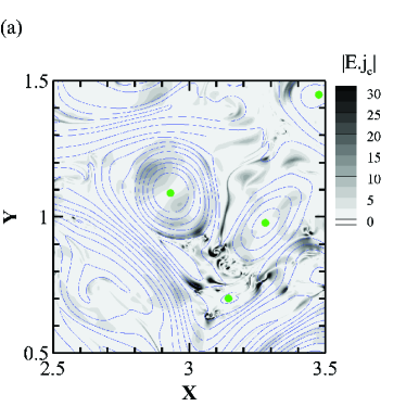
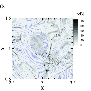
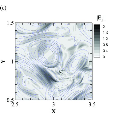
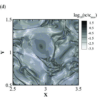
Figure 4: Contour maps of (a) the curvature drift acceleration term $|\boldsymbol{E}\cdot\boldsymbol{j}_{c}|$, (b) the curvature-related component $|\kappa B|$, (c) the perpendicular electric field $|E_{\perp}|$, and (d) the logarithm of the curvature $\kappa$ in a subregion of the whole domain with the blue contour lines showing the magnetic field lines.

The linear anti-correlation between curvature and the square of magnetic field provides a plausible rationale for the similarity between $\kappa B$ and $\kappa$ in Figs. 4(b) and (d) , where here we also exclude from consideration some special points like magnetic island cores and reconnection sites. Although near both magnetic island cores and reconnection sites, the direction of magnetic field changes over very short length scales, corresponding to intense curvature, the product $\kappa B$ is not typically a local maxima at those positions. This seems to be in apparent contradiction to the preceding description of the general trend, that is, the linear anti-correlation between curvature and the square of magnetic field leads to $\kappa B$ in approximately linear relationship with $\sqrt{\kappa}$. However, the measurement of curvature is inevitably limited by the numerical resolution of the simulation. In order to illustrate the effect of grid resolution, we apply a Fourier zero-padding and interpolation technique Servidio et al. (2010) to obtain a $16384^{2}$ array in place of the original $8192^{2}$ array. One can see from Fig. 5(a) that the Fourier zero-padding and interpolation technique improves the accuracy of our measurements of curvature and higher resolution enables resolution of more intense curvature. Also noteworthy from Fig. 5(b) is that the conditional averages of $\kappa$ tend to form a plateau as the magnetic field vanishes, which could be near magnetic island cores and reconnection sites. It is not possible to numerically measure true curvature therein since there will always be noise as approaching these zero-magnetic positions.

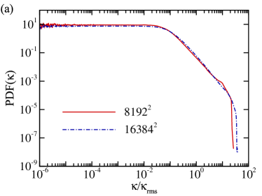
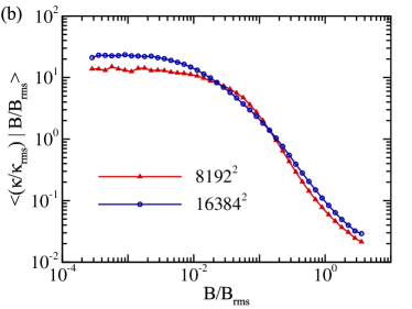
Figure 5: Comparison between $8192^{2}$ resolution and $16384^{2}$ resolution: (a) PDF of magnetic field curvature $\kappa$; (b) Average of magnetic field curvature $\kappa$ conditioned on magnetic magnitude.

Previous studies Dahlin, Drake, and Swisdak (2014, 2017); Li et al. (2017, 2015); Guo et al. (2014); Lu et al. (2018); Wang et al. (2016, 2017) on magnetic reconnection emphasize the prominence of curvature drift acceleration in reconnection exhausts, at ends of contracting magnetic islands and in island merging regions. The importance of this process also emerges by virtue of the curvature analysis here. Figs. 6(a) and (b) show the spatial distributions of the curvature drift acceleration in several subregions, with magnetic island cores marked as green circles and magnetic reconnection sites marked as green stars. On the one hand, the curvature drift acceleration at magnetic island cores and reconnection sites is small, as we have shown, due to the product of the perpendicular electric field $E_{\perp}$ and the curvature-related term $\kappa B$. On the other hand, intense curvature is often found in the vicinity of these positions, thus enhancing the curvature drift acceleration nearby. The analyses we make so far make no specific reference to turbulence. But turbulence and heating processes related to turbulence are frequently implicated in the study of space and astrophysical plasmas Dmitruk, Matthaeus, and Seenu (2004); TenBarge and Howes (2013); Perri et al. (2012); Price et al. (2016); Bandyopadhyay et al. (2018); Yang et al. (2019). Evidently, turbulence, contemporaneous with magnetic reconnection, operates cooperatively in the natural evolution of the magnetic field in these plasmas Retinò et al. (2007); Sundkvist et al. (2007); Matthaeus and Velli (2011); Osman et al. (2014); Zhdankin et al. (2013); Wan et al. (2014). Local flows in turbulence, even though they may not contain a magnetic island core or a reconnection site, may also produce large curvature. To isolate the effect of turbulence, we show regions away from topologically special points in Figs. 6(c) and (d). In comparison with the regions in the proximity of magnetic reconnection sites and magnetic island cores, the observable enhancement of the curvature drift acceleration emerges as well in turbulence-dominant regions, supporting the view that turbulent effects are playing an essential role in particle acceleration.

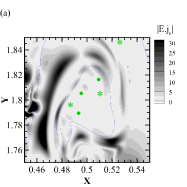
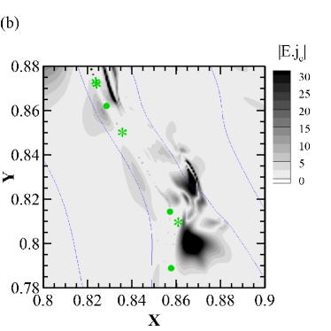
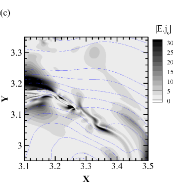
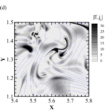
Figure 6: Contour maps of the curvature drift acceleration term $|\boldsymbol{E}\cdot\boldsymbol{j}_{c}|$. (a) and (b): regions with magnetic island cores marked as green circles and magnetic reconnection sites marked as green stars. (c) and (d): regions that do not contain topologically special points. The blue contour lines show the magnetic field lines.

V Further applications

In this section we discuss the properties of magnetic field curvature in two different systems that deviate from the statistically homogeneous, isotropic and two-dimensional MHD: isotropic 3D MHD and 2.5D kinetic plasma.

V.1 3D MHD

The incompressible three-dimensional MHD equations read

$${\frac{\partial\boldsymbol{v}}{\partial t}}+\boldsymbol{v}\cdot\nabla\boldsymbol{v} = -\nabla p^{*}+\boldsymbol{B}\cdot\nabla\boldsymbol{B}+\nu\nabla^{2}\boldsymbol{v},$$ (8)

$${\frac{\partial\boldsymbol{B}}{\partial t}}+\boldsymbol{v}\cdot\nabla\boldsymbol{B} = \boldsymbol{B}\cdot\nabla\boldsymbol{v}+\eta\nabla^{2}\boldsymbol{B},$$ (9)

where $p^{*}$ is the total (kinetic + magnetic) pressure, along with $\nabla\cdot\boldsymbol{v}=\nabla\cdot\boldsymbol{B}=0$. We solve the Fourier-space version of the above equations via a Galerkin spectral method Orszag and Patterson Jr (1972), with $1024$ Fourier modes in each spatial direction. For simplicity, equal viscosity and resistivity $\nu=\eta=4\times 10^{-4}$ are used. The run is a freely decaying problem in periodic cube of size $2\pi$ and has the initially unity fluctuation energy equipartitioned between the kinetic and magnetic components, i.e., $E_{v}=E_{b}=0.5$. The fields are initialized at modes $1\leq|\boldsymbol{k}|\leq 5$ with random phases and fluctuation amplitudes, whose spectra are proportional to $1/\left[1+(k/k_{0})^{11/3}\right]$ with $k_{0}=3$. The cross-helicity is always small. We carry out our analysis on a snapshot near the time of maximum mean square current density.

One can see from Fig. 7 that the PDF of the curvature exhibits power laws for both small-curvature and large-curvature regimes: For small curvature, the PDF is close to linear with $\kappa$, while, for large curvature, it scales as $\kappa^{-2.5}$. Since dimensonality does not enter into the expression in Eq. 5, we expect that the anti-correlation between curvature and magnetic field will hold also in a 3D system. This expectation is confirmed in our simulation, see Fig. 8, which shows that low and high curvature is strongly correlated with small normal force and small magnetic field magnitude, respectively. In analogy with the procedure in 2D, the square of magnetic magnitude $B^{2}$ in 3D MHD should then be distributed following a chi-squared distribution with 3 degrees of freedom. Since the curvature as $\kappa\rightarrow\infty$ scales like $B^{-2}$ as $B^{2}\rightarrow 0$, one can derive the scaling $P(\kappa)\sim\kappa^{-2.5}$ for high curvature. Similar reasoning is applicable to the low-curvature regime. Note that the force $f_{n}$ is confined to the plane orthogonal to the magnetic field. We then assume the PDF of $f_{n}^{2}$ at small values is a chi-squared distribution with 2 degrees of freedom. As $f_{n}\rightarrow 0$, $P(f_{n})\sim f_{n}$, and we recover $P(\kappa)\sim\kappa^{1}$ for low curvature.

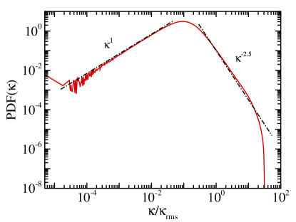
Figure 7: 3D MHD simulation: PDF of the magnetic field curvature $\kappa$ normalized to the root mean square value $\kappa_{\rm rms}$. The PDF has a $\kappa^{1}$ low-curvature regime and a $\kappa^{-2.5}$ high-curvature tail.

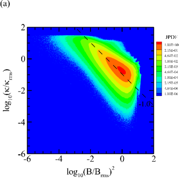
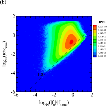
Figure 8: 3D MHD simulation: Joint PDFs of the curvature $\kappa$ and (a) the square of magnetic magnitude $B^{2}$ and (b) the force magnitude $f_{n}$ acting normal to field lines. All quantities are normalized to their respective root mean square values. There are apparent associations between high curvature and low magnetic field and between low curvature and low normal force.

V.2 Kinetic plasma

Plasma turbulence involves structures across a wide range of scales, spanning from macroscopic fluid scales to sub-electron scales. Based on what plasma properties we are interested in studying, a plasma can be treated as tractable models in various limits. MHD model remains a credible approximation for a plasma at scales large enough to be well separated from kinetic effects, while more refined kinetic description is required at kinetic scales. Here we compare results from fully kinetic particle-in-cell (PIC) simulations with those from MHD simulations.

We employ a fully kinetic simulation by P3D Zeiler et al. (2002) in 2.5D geometry (three components of dependent field vectors and a two-dimensional spatial grid). Number density is normalized to a reference number density $n_{r}$ (=1 in this simulation), mass to proton mass $m_{i}$ (=1 in this simulation), charge to proton charge $q_{i}$, and magnetic field to a reference $B_{r}$ (=1 in this run). Length is normalized to the ion inertial length $d_{i}$, time to the ion cyclotron time $\Omega_{i}^{-1}$, velocity to the reference Alfvén speed $v_{Ar}=B_{r}/\left(4\pi m_{i}n_{r}\right)^{1/2}$, and temperature to $T_{r}=m_{i}v_{Ar}^{2}$. The simulation was performed in a periodic domain, whose size is $L=150d_{i}$, with $4096^{2}$ grid points and $3200$ particles of each species per cell ($\sim 107\times 10^{9}$ total particles). The ion to electron mass ratio is $m_{i}/m_{e}=25$, and the speed of light in the simulation is $c=15v_{Ar}$. The run is a decaying initial value problem, starting with uniform density ($n_{0}=1.0$) and temperature of ions and electrons ($T_{0}=0.3$). The uniform magnetic field is $B_{0}=1.0$ directed out of the plane. More details about the simulation can be found in Ref. Yang et al., 2019. We analyze statistics using a snapshot near the time of maximum root mean square electric current density.

One can see from Fig. 9 that the PDF has a $\kappa^{0}$ low-curvature regime and a $\kappa^{-2}$ high-curvature tail. Fig. 10 indicates apparent associations between high curvature and low magnetic field and between low curvature and low normal force. Although the PIC simulation enables the resolution of much smaller scales, the corresponding behavior of curvature is essentially similar to that in 2D MHD. The reasoning advanced in Sec. III might therefore be deemed universal for plasma turbulence.

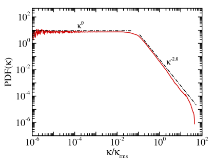
Figure 9: PIC simulation: PDF of the magnetic field curvature $\kappa$ normalized to the root mean square value $\kappa_{\rm rms}$.

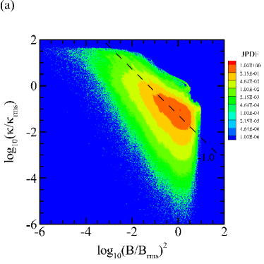
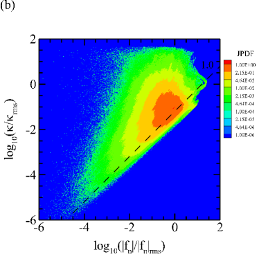
Figure 10: PIC simulation: Joint PDFs of the curvature $\kappa$ and (a) the square of magnetic magnitude $B^{2}$ and (b) the force magnitude $f_{n}$ acting normal to field lines.

VI Conclusions

Curvature characterizes magnetic field lines. For example, both turbulence and magnetic reconnection drive tangled and bent magnetic configurations, corresponding to intense curvature. We can therefore analyze curvature properties to improve understanding of the curvature drift mechanism, often implicated in particle acceleration. In this work, we have clarified the dependence between high curvature and low magnetic field. In particular, high curvature $\kappa$ is statistically scaled as $B^{-2}$, thus generating the power-law tails of the PDF of curvature. The curvature drift term, responsible for particle energization, is found to be strongly associated with the scalar curvature. It is active in high-curvature positions which could be attributed to turbulence and magnetic reconnection. We have not attempted to quantify the relative strength of these two kinds of acceleration processes here.

The simulations used here include two-dimensional MHD and three-dimensional MHD, but it does not necessarily make a reference to the dimensionality when arriving at Eqs. 5 and 7, in order to maintain as broad a context as possible. It is therefore expected that the relevant statistical features are substantially analogous in 3D and 2D. Indeed, the anti-correlation between high curvature and low magnetic field applies as well to the 3D case. Also noteworthy is its application for kinetic plasma based on PIC simulation. However, we should make it clear that this work is neither complete in its coverage nor exhaustive of possibilities. The curvature drift mechanism we study is only one possibility for particle acceleration and other mechanisms have not been addressed herein.

VII Acknowledgments

This work has been supported by NSFC Grant Nos. 91752201 and 11672123; the Shenzhen Science and Technology Innovation Committee (Grant No. JCYJ20170412151759222). Yan Yang is supported by the Presidential Excellence Postdoctoral Fellowship from the Southern Univeristy of Science and Technology. WHM is supported in part by NASA under the MMS Theory and Modeling team (NNX14AC39G), and the Parker Solar Probe mission (Princeton subcontract SUB0000165). We acknowledge computing support provided by Center for Computational Science and Engineering of Southern University of Science and Technology.

References

- Parker (1979) E. N. Parker, Cosmical Magnetic Fields: Their Origin and Activity (Oxford, UK, 1979).
- Newcomb (1958) W. A. Newcomb, Annals of Physics 3, 347 (1958).
- Jokipii (1966) J. R. Jokipii, The Astrophysical Journal 146, 480 (1966).
- Jokipii and Parker (1969) J. Jokipii and E. Parker, The Astrophysical Journal 155, 777 (1969).
- Matthaeus et al. (1995) W. Matthaeus, P. Gray, D. Pontius Jr, and J. Bieber, Physical review letters 75, 2136 (1995).
- Northrop (1961) T. G. Northrop, Annals of Physics 15, 79 (1961).
- Drake et al. (2006) J. Drake, M. Swisdak, H. Che, and M. Shay, Nature 443, 553 (2006).
- Hoshino et al. (2001) M. Hoshino, T. Mukai, T. Terasawa, and I. Shinohara, Journal of Geophysical Research: Space Physics 106, 25979 (2001).
- Egedal, Daughton, and Le (2012) J. Egedal, W. Daughton, and A. Le, Nature Physics 8, 321 (2012).
- Oka et al. (2010) M. Oka, T.-D. Phan, S. Krucker, M. Fujimoto, and I. Shinohara, The Astrophysical Journal 714, 915 (2010).
- Pritchett (2006) P. Pritchett, Journal of Geophysical Research: Space Physics 111 (2006).
- Dahlin, Drake, and Swisdak (2014) J. Dahlin, J. Drake, and M. Swisdak, Physics of Plasmas 21, 092304 (2014).
- Dahlin, Drake, and Swisdak (2017) J. Dahlin, J. Drake, and M. Swisdak, Physics of Plasmas 24, 092110 (2017).
- Li et al. (2017) X. Li, F. Guo, H. Li, and G. Li, The Astrophysical Journal 843, 21 (2017).
- Li et al. (2015) X. Li, F. Guo, H. Li, and G. Li, The Astrophysical Journal Letters 811, L24 (2015).
- Guo et al. (2014) F. Guo, H. Li, W. Daughton, and Y.-H. Liu, Physical Review Letters 113, 155005 (2014).
- Lu et al. (2018) Q. Lu, H. Wang, K. Huang, R. Wang, and S. Wang, Physics of Plasmas 25, 072126 (2018).
- Wang et al. (2016) H. Wang, Q. Lu, C. Huang, and S. Wang, The Astrophysical Journal 821, 84 (2016).
- Wang et al. (2017) H. Wang, Q. Lu, C. Huang, and S. Wang, Physics of Plasmas 24, 052113 (2017).
- Wan et al. (2013) M. Wan, W. H. Matthaeus, S. Servidio, and S. Oughton, Physics of Plasmas 20, 042307 (2013).
- Braun, De Lillo, and Eckhardt (2006) W. Braun, F. De Lillo, and B. Eckhardt, Journal of Turbulence , N62 (2006).
- Xu, Ouellette, and Bodenschatz (2007) H. Xu, N. T. Ouellette, and E. Bodenschatz, Phys. Rev. Lett. 98, 050201 (2007).
- Ouellette and Gollub (2007) N. T. Ouellette and J. P. Gollub, Physical review letters 99, 194502 (2007).
- Ouellette and Gollub (2008) N. T. Ouellette and J. P. Gollub, Physics of Fluids 20, 064104 (2008).
- Scagliarini (2011) A. Scagliarini, Journal of Turbulence , N25 (2011).
- Kadoch et al. (2011) B. Kadoch, D. del Castillo-Negrete, W. J. Bos, and K. Schneider, Physical Review E 83, 036314 (2011).
- Yang et al. (2013) Y. Yang, J. Wang, Y. Shi, Z. Xiao, X. He, and S. Chen, Physical review letters 110, 064503 (2013).
- Servidio et al. (2010) S. Servidio, W. Matthaeus, M. Shay, P. Dmitruk, P. Cassak, and M. Wan, Physics of Plasmas 17, 032315 (2010).
- Dmitruk, Matthaeus, and Seenu (2004) P. Dmitruk, W. H. Matthaeus, and N. Seenu, Astrophys. J. 617, 667 (2004).
- TenBarge and Howes (2013) J. M. TenBarge and G. G. Howes, Astrophys. J. Lett. 771, L27 (2013).
- Perri et al. (2012) S. Perri, M. L. Goldstein, J. C. Dorelli, and F. Sahraoui, Phys. Rev. Lett. 109, 191101 (2012).
- Price et al. (2016) L. Price, M. Swisdak, J. Drake, P. Cassak, J. Dahlin, and R. Ergun, Geophysical Research Letters 43, 6020 (2016).
- Bandyopadhyay et al. (2018) R. Bandyopadhyay, A. Chasapis, R. Chhiber, T. Parashar, B. Maruca, W. Matthaeus, S. Schwartz, S. Eriksson, O. Le Contel, H. Breuillard, et al., The Astrophysical Journal 866, 81 (2018).
- Yang et al. (2019) Y. Yang, M. Wan, W. H. Matthaeus, L. Sorriso-Valvo, T. N. Parashar, Q. Lu, Y. Shi, and S. Chen, Monthly Notices of the Royal Astronomical Society 482, 4933 (2019).
- Retinò et al. (2007) A. Retinò, D. Sundkvist, A. Vaivads, F. Mozer, M. André, and C. J. Owen, Nature Phys. 3, 235 (2007).
- Sundkvist et al. (2007) D. Sundkvist, A. Retinò, A. Vaivads, and S. D. Bale, Phys. Rev. Lett. 99, 025004 (2007).
- Matthaeus and Velli (2011) W. Matthaeus and M. Velli, Space science reviews 160, 145 (2011).
- Osman et al. (2014) K. Osman, W. Matthaeus, J. Gosling, A. Greco, S. Servidio, B. Hnat, S. C. Chapman, and T. Phan, Physical Review Letters 112, 215002 (2014).
- Zhdankin et al. (2013) V. Zhdankin, D. A. Uzdensky, J. C. Perez, and S. Boldyrev, The Astrophysical Journal 771, 124 (2013).
- Wan et al. (2014) M. Wan, A. F. Rappazzo, W. H. Matthaeus, S. Servidio, and S. Oughton, The Astrophysical Journal 797, 63 (2014).
- Orszag and Patterson Jr (1972) S. A. Orszag and G. Patterson Jr, Physical Review Letters 28, 76 (1972).
- Zeiler et al. (2002) A. Zeiler, D. Biskamp, J. F. Drake, B. N. Rogers, M. A. Shay, and M. Scholer, J. Geophys. Res. 107, 1230 (2002).