Analysis of sparse grid multilevel estimators for multi-dimensional Zakai equations

Abstract

In this article, we analyse the accuracy and computational complexity of estimators for expected functionals of the solution to multi-dimensional parabolic stochastic partial differential equations (SPDE) of Zakai-type. Here, we use the Milstein scheme for time integration and an alternating direction implicit (ADI) splitting of the spatial finite difference discretisation, coupled with the sparse grid combination technique and multilevel Monte Carlo sampling (MLMC). In the two-dimensional case, we find by detailed Fourier analysis that for a root-mean-square error (RMSE) $\varepsilon$, MLMC on sparse grids has the optimal complexity $O(\varepsilon^{-2})$, whereas MLMC on regular grids has $O(\varepsilon^{-2}(\log\varepsilon)^{2})$, standard MC on sparse grids $O(\varepsilon^{-7/2}(|\log\varepsilon|)^{5/2})$, and MC on regular grids $O(\varepsilon^{-4})$. Numerical tests confirm these findings empirically. We give a discussion of the higher-dimensional setting without detailed proofs, which suggests that MLMC on sparse grids always leads to the optimal complexity, standard MC on sparse grids has a fixed complexity order independent of the dimension (up to a logarithmic term), whereas the cost of MLMC and MC on regular grids increases exponentially with the dimension.

1 Introduction

The focus of this paper is the efficient simulation of the two-dimensional SPDE

$$\mathrm{d}v = Lv\,\mathrm{d}t-\sqrt{\rho_{x}}\frac{\partial v}{\partial x}\,\mathrm{d}W_{t}^{x}-\sqrt{\rho_{y}}\frac{\partial v}{\partial y}\,\mathrm{d}W_{t}^{y}$$ (1.1)

for $x,y\in\mathbb{R},\ 0<t\leq T$, subject to the Dirac initial datum

$$v(0,x,y)=\delta(x-x_{0})\otimes\delta(y-y_{0})$$ (1.2)

for given $x_{0}$ and $y_{0}$, where $W=(W^{x},\,W^{y})$ is a two-dimensional standard Brownian motion with correlation $\rho_{xy}$ on a probability space $(\Omega,\mathcal{F},\mathbb{P})$,

$$Lv = -\mu_{x}\frac{\partial v}{\partial x}-\mu_{y}\frac{\partial v}{\partial y}+\frac{1}{2}\bigg{(}\frac{\partial^{2}v}{\partial x^{2}}+2\sqrt{\rho_{x}\rho_{y}}\rho_{xy}\frac{\partial^{2}v}{\partial x\partial y}+\frac{\partial^{2}v}{\partial y^{2}}\bigg{)},$$

$\mu_{x},\mu_{y}$ and $0\leq\rho_{x},\rho_{y}<1$, $-1\leq\rho_{xy}\leq 1$ are real-valued parameters.

This is a special case of the Zakai equation from stochastic filtering where $v$ describes the distribution of the filter given a signal process $W$ (see [1, 9]).

A classical result states that, for a class of SPDEs including (1.1), with initial condition in $L_{2}$, there exists a unique solution $v\in L_{2}(\Omega\times(0,T),\mathcal{F},L_{2}(\mathbb{R}^{2}))$ [13]. This does not include Dirac initial data (1.2), but in fact, the solution to (1.1) and (1.2) can be analytically derived as the smooth (in $x$ and $y$) function

$$v(T,x,y)=\frac{\exp\Big{(}-\frac{\big{(}x-x_{0}-\mu_{x}T-\sqrt{\rho_{x}}W_{T}^{x}\big{)}^{2}}{2(1-\rho_{x})T}-\frac{\big{(}y-y_{0}-\mu_{y}T-\sqrt{\rho_{y}}W_{T}^{y}\big{)}^{2}}{2(1-\rho_{y})T}\Big{)}}{2\pi\sqrt{(1-\rho_{x})(1-\rho_{y})}\,T}\,.$$ (1.3)

More commonly, however, such a closed-form solution is not available, for instance in the case of variable coefficients. We will focus on (1.1) for the analysis, but the numerical methods we investigate apply similarly to such a wider class.

There is a large body of recent literature on the numerical solution of SPDEs. Most closely related to the present work, Giles and Reisinger in [8] used an explicit Milstein finite difference approximation to the solution of the one-dimensional SPDE

$$\mathrm{d}v=-\mu\frac{\partial v}{\partial x}\,\mathrm{d}t+\frac{1}{2}\frac{\partial^{2}v}{\partial x^{2}}\,\mathrm{d}t-\sqrt{\rho}\frac{\partial v}{\partial x}\,\mathrm{d}W_{t},\qquad(t,x)\in(0,T)\times\mathbb{R},$$ (1.4)

where $T>0$, $W$ is a standard Brownian motion, and $\mu$ and $0\leq\rho<1$ are real-valued parameters; [17] extended the discretisation to an implicit method on the basis of the $\sigma$-$\theta$ time-stepping scheme. This 1-d SPDE (1.4) has also been used to model default risk in large credit portfolios (see [4]).

For the 2-d SPDE (1.1), we will use an implicit method such that under some constraints on $\rho_{x},\rho_{y},\rho_{xy}$, the scheme is unconditionally mean-square stable. Furthermore, we use an Alternating Direction Implicit (ADI) factorisation which is more convenient computationally than a purely implicit scheme, and is also unconditionally mean-square stable (see [19]).

We consider the following functional of the solution,

$$P_{t}=\int_{0}^{\infty}\int_{0}^{\infty}v(t,x,y)\,\mathrm{d}x\,\mathrm{d}y,$$ (1.5)

which is a two-dimensional version of the loss in [4, 8] which represents the proportion of the defaulted firms there. In the context of filtering, $P_{t}$ is related to the cumulative distribution function of the filter given the signal.

The functional in (1.5) is a special case of more general linear and nonlinear functionals of the form

$$\int_{-\infty}^{\infty}\int_{-\infty}^{\infty}f(x,y)v(t,x,y)\,\mathrm{d}x\,\mathrm{d}y,\qquad g\Big{(}\int_{0}^{\infty}\int_{0}^{\infty}v(t,x,y)\,\mathrm{d}x\,\mathrm{d}y\Big{)},$$

with $f$ being the Heaviside function and $g$ the identity in the case of $P_{t}$. Preliminary derivations indicate that our analysis may be extended from $P_{t}$ to these cases for sufficiently smooth $f$ and $g$, by judicious multivariate Taylor expansion, but this involves exceedingly lengthy calculus and is beyond the scope of this work.

A classical approach to approximating $\mathbb{E}[P_{t}]$ is the standard Monte Carlo method, using a suitable approximation scheme for (1.1) and sampling of $W$ on a discrete time mesh. For the SPDE (1.1) and standard schemes, to achieve a root mean square error (RMSE) $\varepsilon$, this requires an overall computational cost $O(\varepsilon^{-4})$, as we require $O(\varepsilon^{-2})$ samples, $O(\varepsilon^{-1})$ time steps (e.g., for the Euler-Maruyama scheme with weak order 1), and $O(\varepsilon^{-1/2})$ mesh points in each direction (e.g., for central difference schemes with order 2). One way to reduce the cost is the MLMC method (see [6]) by using the SPDE solution on paths with a coarse timestep and spatial mesh as a control variate of solutions on paths with a fine timestep and mesh. As a result, for a fixed accuracy $\varepsilon$, the cost can be reduced significantly to $O(\varepsilon^{-2}(\log\varepsilon)^{2})$ by standard MLMC methodology as in [8]. However, this complexity of the MLMC method is not optimal as in the one-dimensional case in [8]. The reason is that the cost of each sample on higher levels increases with the same order as the variance decays. Moreover, the total cost of MLMC increases exponentially in the dimension.

The approach taken here is to approximate the SPDE (1.1) by the sparse grid combination technique. Sparse grids were first introduced to solve high-dimensional PDEs on a tensor product space in [20]. The error bounds in [2] show that sparse finite element approximations can alleviate the curse of dimensionality in the numerical implementation of certain elliptic PDEs with sufficiently smooth solutions. In contrast to the finite element method, the combination technique, first introduced in [10], decomposes the solution into contributions from simple tensor product grids with different resolutions in each dimension. For a survey of methods and early results see [3]. The analysis in [15] and [16] shows that the computational cost for the combination technique applied to the Poisson problem with sufficient regularity is independent of the dimension, up to a logarithmic term, for finite elements and finite differences, respectively. Hendricks, Ehrhardt and Günther combine the sparse grid combination technique with the ADI scheme for diffusion equations in [12].

This sparse grid method has been extended to multi-index Monte Carlo (MIMC) in the context of SPDEs in [11]. MIMC can be viewed as the sparse grid combination technique applied to equations with stochasticity, with optimised number of samples for the individual terms in the combination formula (the “hierarchical surpluses”), akin MLMC. Giles, Kuo and Sloan summarised these ideas applied to elliptic PDEs with finite-dimensional uncertainty in the coefficients in [7]. The MIMC method was applied in [18] to a 1-d SPDE (1.4), where the timestep and space mesh are coupled for stability. However, optimal complexity is not achieved in this space-time method.

In this paper, given a fixed timestep and Brownian path, we solve the SPDE using the sparse grid combination technique in space. Then, to evaluate $\mathbb{E}[P_{t}]$, we use $M$ independent samples of the hierarchical surpluses and calculate the average. The benefit here is that with a RMSE $\varepsilon$, the total cost is fixed with $O(\varepsilon^{-7/2})$ up to a logarithmic term, as the cost for one sample is $O(\varepsilon^{-3/2}|\log\varepsilon|^{5(d-1)/2})$, and the number of samples needed is $M=O(\varepsilon^{-2})$. Hence, this will improve on the complexity of the MLMC method, whose total cost is $O(\varepsilon^{-1-d/2})$, when the dimension $d>5$.

To recover the optimal complexity $O(\varepsilon^{-2})$, we further combine the sparse combination technique and MLMC, in a different way from standard MIMC. In this way, the total cost is $O(\varepsilon^{-2})$ independent of dimension.

The rest of this article is structured as follows. We define the approximation schemes in Section 2. Section 3 gives a Fourier analysis of the sparse combination estimators. Section 4 shows numerical experiments confirming the above findings, and Section 5 generalises the problem to higher dimensions. Section 6 offers conclusions and directions for further research.

2 Approximation and main results

For simplicity of presentation, we initially restrict ourselves with the description of the schemes and their analysis to the two-dimensional case. The extension to higher dimensions is discussed in Section 5.

Moreover, we focus on the case of constant coefficients as in (1.1) and the functional (1.5). While the numerical method itself is directly applicable to the variable coefficient case and more general functionals, the Fourier analysis we perform is tailored to the present setting.

2.1 Semi-implicit Milstein finite difference scheme

We use a spatial grid with uniform spacing $h_{x},\,h_{y}>0$, and let $V_{i,j}^{n}$ be the approximation to $v(nk,ih_{x},jh_{y})$, $n=1,\ldots,N$, $i,j\in\mathbb{Z}$. We assume for simplicity that $i_{0}:=x_{0}/h_{x}$ and $j_{0}:=y_{0}/h_{y}$ are integers. Then we approximate $v(0,x,y)=\delta(x-x_{0})\otimes\delta(y-y_{0})$ by

$$V_{i,j}^{0}=h_{x}^{-1}h_{y}^{-1}\delta_{(i_{0},\,j_{0})}=\begin{cases}h_{x}^{-1}h_{y}^{-1},\quad&i=i_{0},\ j=j_{0},\\ 0,&\text{otherwise}.\end{cases}$$ (2.1)

We use the semi-implicit Milstein scheme to approximate (1.1), proposed in [19]:

$$\!\!\!\!\bigg{(}I+\frac{\mu_{x}k}{2h_{x}}D_{x}+\frac{\mu_{y}k}{2h_{y}}D_{y}-\frac{k}{2h_{x}^{2}}D_{xx}-\frac{k}{2h_{y}^{2}}D_{yy}\!\bigg{)}V^{n+1}\!=\bigg{(}\!I\!-\!\frac{\sqrt{\rho_{x}k}Z_{n,x}}{2h_{x}}D_{x}\!-\!\frac{\sqrt{\rho_{y}k}\widetilde{Z}_{n,y}}{2h_{y}}D_{y}$$ (2.2)

$$+\frac{\rho_{x}k(Z_{n,x}^{2}\!\!-\!1)}{8h_{x}^{2}}D_{x}^{2}\!+\!\frac{\rho_{y}k(\widetilde{Z}_{n,y}^{2}\!\!-\!1)}{8h_{y}^{2}}D_{y}^{2}\!+\!\frac{\sqrt{\rho_{x}\rho_{y}}kZ_{n,x}\widetilde{Z}_{n,y}}{4h_{x}h_{y}}D_{xy}\!\bigg{)}\!V^{n}$$

$$=:M_{n}V^{n},$$

where $M$ is a random operator and

$$(D_{x}V)_{i,j}=V_{i+1,j}-V_{i-1,j},\qquad\qquad\qquad\quad\ \;(D_{y}V)_{i,j}=V_{i,j+1}-V_{i,j-1},$$

$$(D_{xx}V)_{i,j}=V_{i+1,j}-2V_{i,j}+V_{i-1,j},\quad\qquad\quad\;\,(D_{yy}V)_{i,j}=V_{i,j+1}-2V_{i,j}+V_{i,j-1},$$

$$(D_{xy}V)_{i,j}=V_{i+1,j+1}-V_{i-1,j+1}-V_{i+1,j-1}+V_{i-1,j-1},$$

and $\widetilde{Z}_{n}^{y}=\rho_{xy}Z_{n}^{x}+\sqrt{1-\rho_{xy}^{2}}Z_{n}^{y}$ with $Z_{n}^{x},Z_{n}^{y}\sim N(0,1)$ independent normals. Briefly, the terms on the left-hand side of (2.2) correspond to the implicit approximation of the operator $L$ in (1.1); the second and third terms on the right-hand side are the Euler-Maruyama approximation of the stochastic integral; and the last three terms the Milstein correction for strong first order 1. Note that the cross-derivative term on the left-hand side cancels out with a Milstein term, as detailed in [19].

To save computational cost, we combine the scheme with an Alternating Direction Implicit (ADI) factorisation [14],

$$\bigg{(}I+\frac{\mu_{x}k}{2h_{x}}D_{x}-\frac{k}{2h_{x}^{2}}D_{xx}\bigg{)}\bigg{(}I+\frac{\mu_{y}k}{2h_{y}}D_{y}-\frac{k}{2h_{y}^{2}}D_{yy}\bigg{)}V^{n+1}=M_{n}V^{n}\!.$$ (2.3)

A detailed analysis of the $L_{2}$ stability and convergence of these schemes can be found in [19]. Here, we state the main result which is relevant here. We make the following technical assumptions throughout:

$$2\rho_{x}^{2}(1+2|\rho_{xy}|) \leq 1,\quad 2\rho_{y}^{2}(1+2|\rho_{xy}|) \leq 1,\quad 2\rho_{x}\rho_{y}(3\rho_{xy}^{2}+2|\rho_{xy}|+1) \leq 1.$$ (2.4)

Theorem 2.1 (Corollary 2.1 in [19])

Let $\lambda>0$ be fixed and (2.4) be satisfied. Then there exists $C>0$ such that for any $k,h_{x},h_{y}$ with

$$k/\min\{h_{x}^{2},h_{y}^{2}\}\leq\lambda,$$ (2.5)

for the solution to the implicit Milstein scheme (2.2),

$$\sqrt{\mathbb{E}\big{[}|V_{i,j}^{N}-v(T,ih_{x},jh_{y})|^{2}\big{]}}\leq C(h_{x}^{2}+h_{y}^{2}).$$

This convergence result also holds for the ADI scheme (2.3).

2.2 Sparse combination estimators

Now we consider the specific functional

$$P_{T}=\int_{0}^{\infty}\int_{0}^{\infty}v(T,x,y)\,\mathrm{d}x\,\mathrm{d}y,$$ (2.6)

as discussed in the introduction, where $v$ is the solution to (1.1) and (1.2).

By introducing integer multi-indices $\bm{l}=(l_{1},l_{2})\in\mathbb{N}^{2}$ as the refinement levels of the spatial mesh in dimensions $x$ and $y$, respectively, we denote by $P_{(l_{1},\,l_{2})}^{N}$ the discrete approximations to $P$ with mesh sizes $h_{x}=h_{0}\cdot 2^{-l_{1}}$, $h_{y}=h_{0}\cdot 2^{-l_{2}}$, and fixed timestep $k$ with $k\leq\lambda\min\{h_{x}^{2},h_{y}^{2}\}$. Let $N=T/k$. We then use the trapezoidal approximation

$$P_{(l_{1},\,l_{2})}^{N} =h_{x}h_{y}\sum_{i=1}^{\infty}\sum_{j=1}^{\infty}V_{i,j}^{N}+\frac{h_{x}}{2}\sum_{j=1}^{\infty}V_{0,j}^{N}+\frac{h_{y}}{2}\sum_{i=1}^{\infty}V_{i,0}^{N}+\frac{1}{4}h_{x}h_{y}V_{0,0}^{N},$$ (2.7)

where $V_{i,j}^{N}$ is the solution to (2.2).

Proposition 2.1

Assume (2.4) holds. Let $P$ be given by (2.6) and $P^{N}_{(l_{1},\,l_{2})}$ by (2.7). Then for fixed $\lambda>0$ there exists $C>0$ such that for any $(l_{1},l_{2})\in\mathbb{N}_{0}^{2}$, $k\leq\lambda\min\{h_{x}^{2},h_{y}^{2}\}$,

$$\sqrt{\mathbb{E}\left[\lvert P^{N}_{(l_{1},\,l_{2})}-P\rvert^{2}\right]}\leq C(h_{x}^{2}+h_{y}^{2}),$$ (2.8)

where $h_{x}=h_{0}\cdot 2^{-l_{1}},\,h_{y}=h_{0}\cdot 2^{-l_{2}}$, $N=T/k$.

Proof Similar to Proposition 2.2 in [18]. $\Box$

Let $\Delta_{i}$ be the first-order difference operator along directions $i=1,2$, defined as

$$\Delta_{i}P_{\bm{l}}^{N}=\begin{cases}P_{\bm{l}}^{N}-P_{\bm{l}-\bm{e}_{i}}^{N},\quad&\text{if}\ l_{i}>0,\\ P_{\bm{l}}^{N}&\text{if}\ l_{i}=0,\end{cases}$$ (2.9)

with $\bm{e}_{i}$ the canonical unit vectors in $\mathbb{R}^{2}$, i.e., $(\bm{e}_{i})_{j}=\delta_{ij}$, and $\bm{l}=(l_{1},l_{2})$. We also define the first-order mixed difference operator $\Delta=\Delta_{1}\otimes\Delta_{2}$. Hence, for $l_{1}>0,l_{2}>0$,

$$\Delta P_{(l_{1},\,l_{2})}^{N}=P_{(l_{1},\,l_{2})}^{N}-P_{(l_{1},\,l_{2}-1)}^{N}-P_{(l_{1}-1,\,l_{2})}^{N}+P_{(l_{1}-1,\,l_{2}-1)}^{N}.$$ (2.10)

We will prove in Section 3.3 the following theorem.

Theorem 2.2

Assume (2.4) holds. Let $h_{x}=h_{0}\cdot 2^{-l_{1}},\ h_{y}=h_{0}\cdot 2^{-l_{2}}$, and for any fixed $\lambda>0$, $k/\min\{h_{x}^{2},h_{y}^{2}\}\leq\lambda$, $N=T/k$. Then for $\Delta P^{N}_{(l_{1},\,l_{2})}$ from (2.10),

$$\Big{|}\mathbb{E}\left[\Delta P^{N}_{(l_{1},\,l_{2})}\right]\Big{|}=O(h_{x}^{2}h_{y}^{2}),\qquad\mathbb{E}\Big{[}\left|\Delta P^{N}_{(l_{1},\,l_{2})}\right|^{2}\Big{]}=O(h_{x}^{4}h_{y}^{4}).$$ (2.11)

Proof See Section 3.3. $\Box$

Remark 2.1

We emphasise that (2.11) does not follow from (2.8), but ascertains essentially that the difference operator cancels out any terms in the error expansion which depend on $h_{x}$ or $h_{y}$ alone. Establishing this property, which depends on the regularity of the problem, is the crucial step for the application of the sparse combination technique in the deterministic case of PDEs (see [10, 3, 16]). It is precisely the condition required for the Multi-Index Monte Carlo method of [11]. Indeed, the approach here is interpretable as a specific multi-index decomposition applied to the spatial variables, treating time separately.

Corollary 2.1

With the same setting as in Theorem 2.2, the first order differences of $P^{N}_{(l_{1},l_{2})}$ derived from (2.7) have the first and second moments

$$\Big{|}\mathbb{E}\left[\Delta_{1}P^{N}_{(l_{1},\,l_{2})}\right]\Big{|}=O(h_{x}^{2}),\qquad\mathbb{E}\Big{[}\left|\Delta_{1}P^{N}_{(l_{1},\,l_{2})}\right|^{2}\Big{]}=O(h_{x}^{4}),$$

$$\Big{|}\mathbb{E}\left[\Delta_{2}P^{N}_{(l_{1},\,l_{2})}\right]\Big{|}=O(h_{y}^{2}),\qquad\mathbb{E}\Big{[}\left|\Delta_{2}P^{N}_{(l_{1},\,l_{2})}\right|^{2}\Big{]}=O(h_{y}^{4}).$$

Following the ideas in [3, 11], given a sequence of index sets $\mathcal{I}_{l}=\{(l_{1},\,l_{2})\in\mathbb{N}_{0}^{2}:\,l_{1}+l_{2}\leq l+1\}$, the approximation on level $l$ is defined as

$$P_{l}^{N}=\sum_{(l_{1},\,l_{2})\in\mathcal{I}_{l}}\Delta P_{(l_{1},\,l_{2})}^{N}.$$ (2.12)

Note that we use the same $k$ for all $\Delta P_{(l_{1},\,l_{2})}^{N}$, $(l_{1},\,l_{2})\in\mathcal{I}_{l}$. We have the following.

Theorem 2.3

Assume (2.4) holds. Let $k\leq\lambda\,h_{0}^{2}\,2^{-2l}$ for a fixed $\lambda>0$, $N=T/k$, $P$ given by (2.6) and $P_{l}^{N}$ given by (2.12). Then

$$\sqrt{\mathbb{E}\left[\lvert P^{N}_{l}-P\rvert^{2}\right]}=O(l\,2^{-2l}).$$ (2.13)

Proof See Section 3.4. $\Box$

The standard Monte Carlo estimator for $\mathbb{E}\big{[}P_{l}^{N}\big{]}$ using $M$ samples is defined as

$$\widehat{Y}=\frac{1}{M}\sum_{m=1}^{M}\sum_{(l_{1},\,l_{2})\in\mathcal{I}_{l}}\!\!\!\Big{(}\Delta\widehat{P}_{(l_{1},\,l_{2})}^{N}\Big{)}^{(m)},$$ (2.14)

where $\Big{(}\Delta\widehat{P}_{(l_{1},\,l_{2})}^{N}\Big{)}^{(m)}$ is the $m$-th sample for the difference on spatial grid level $(l_{1},\,l_{2})$ of the SPDE approximation using $N$ time steps.

To reduce the bias below $\varepsilon$, we can choose $l=\big{[}\frac{1}{2}(-\log_{2}\varepsilon+\log_{2}|\log\varepsilon|)\big{]}$, where $[\,\cdot\,]$ is the closest integer. Since $k\leq\lambda h_{0}^{2}2^{-2l}=O(2^{-2l})$, the computational cost for one sample of $P_{(l_{1},l_{2})}^{N}$ is

$$W=\sum_{l_{1}+l_{2}\leq l+1}2^{l_{1}+l_{2}}\cdot O(k^{-1})=O(l\,2^{3l})=O\big{(}\varepsilon^{-\frac{3}{2}}|\log\varepsilon|^{\frac{5}{2}}\big{)}.$$

Using standard Monte Carlo sampling, we need $M=O(\varepsilon^{-2})$ samples to reduce the variance below $\varepsilon^{2}$, hence the total computational cost to achieve a RMSE $\varepsilon$ is

$$W=O\big{(}\varepsilon^{-\frac{7}{2}}|\log\varepsilon|^{\frac{5}{2}}\big{)}.$$

2.3 Sparse combination MLMC estimators

Next, we combine the sparse grid combination technique with the MLMC method. We will show that this combination leads to the optimal complexity $O(\varepsilon^{-2})$.

Let $P_{l}\coloneqq P_{l}^{N_{l}}$ be an approximation to $P$ as in (2.12) using a numerical discretisation with timestep $k_{l}$ and index set $\mathcal{I}_{l}$, where

$$\mathcal{I}_{l}=\{(l_{1},\,l_{2})\in\mathbb{N}_{0}^{2}:\,l_{1}+l_{2}\leq l+1\},\qquad k_{l}=k_{0}\cdot 2^{-2l},\qquad N_{l}=\frac{T}{k_{l}}.$$

For $(l_{1},\,l_{2})\in\mathcal{I}_{l}$, the mesh sizes are $h_{x}^{(l_{1})}=h_{0}\cdot 2^{-l_{1}}$, $h_{y}^{(l_{2})}=h_{0}\cdot 2^{-l_{2}}$. By using different levels of refinement, we have the following identity:

$$\mathbb{E}[P]=\mathbb{E}[P_{0}]+\sum_{l=1}^{\infty}\mathbb{E}[P_{l}-P_{l-1}].$$

Then we define the difference operators (acting on the level)

$$\delta P_{l}=P_{l}-P_{l-1}=\sum_{(l_{1},\,l_{2})\in\mathcal{I}_{l}}\Delta P_{(l_{1},\,l_{2})}^{N_{l}}-\sum_{(l_{1},\,l_{2})\in\mathcal{I}_{l-1}}\Delta P_{(l_{1},\,l_{2})}^{N_{l-1}},\quad l\geq 0,$$ (2.15)

where we denote $P_{-1}\coloneqq 0$. Thus, the approximation $\mathbb{E}[P_{l^{\ast}}]$ to $\mathbb{E}[P]$ at level $l^{\ast}$ is

$$\sum_{l=0}^{l^{\ast}}\mathbb{E}[\delta P_{l}]=\mathbb{E}\bigg{[}\sum_{(l_{1},\,l_{2})\in\mathcal{I}_{0}}\Delta P_{(l_{1},\,l_{2})}^{N_{0}}\bigg{]}+\sum_{l=1}^{l^{\ast}}\mathbb{E}\bigg{[}\sum_{(l_{1},\,l_{2})\in\mathcal{I}_{l}}\Delta P_{(l_{1},\,l_{2})}^{N_{l}}-\sum_{(l_{1},\,l_{2})\in\mathcal{I}_{l-1}}\Delta P_{(l_{1},\,l_{2})}^{N_{l-1}}\bigg{]}.$$

Therefore, instead of directly simulating $P_{l^{\ast}}$, we simulate $\delta P_{l},\,l=0,1,\ldots,l^{\ast}$ separately. The key point is that we use the same Brownian path for $P_{l}$ and $P_{l-1}$ to calculate $\delta P_{l}=P_{l}-P_{l-1}$ such that the variance is considerably reduced. We have:

$$\mathbb{E}[\delta P_{l}]\leq C_{1}\cdot l\,2^{-2l},\quad\mathrm{Var}[\delta P_{l}]\leq C_{2}\cdot l^{2}\,2^{-4l},\quad\mathrm{Cost}[\delta P_{l}]\leq C_{3}\cdot l\,2^{3l},$$ (2.16)

where the first two inequalities follow from Theorem 2.3 and the third is immediate.

Let $\widehat{Y}_{l}$ be an estimator for $\mathbb{E}\big{[}\delta P_{l}\big{]}$ using $M_{l}$ independent samples $\delta\widehat{P}_{l}^{(m)}$ of $\delta P_{l}$,

$$\widehat{Y}_{l}=\frac{1}{M_{l}}\sum_{m=1}^{M_{l}}\delta\widehat{P}_{l}^{(m)},\quad l=1,\ldots,l^{\ast}.$$

The MLMC estimator is then defined as $\widehat{P}_{l^{\ast}}\coloneqq\sum_{l=0}^{l^{\ast}}\widehat{Y}_{l}$ or

$$\widehat{P}_{l^{\ast}} = \frac{1}{M_{0}}\sum_{m=1}^{M_{0}}\sum_{(l_{1},\,l_{2})\in\mathcal{I}_{0}}\!\!\!\Big{(}\Delta\widehat{P}_{(l_{1},\,l_{2})}^{N_{0}}\Big{)}^{(m)}+$$

$$\qquad\qquad\sum_{l=1}^{l^{\ast}}\frac{1}{M_{l}}\sum_{m=1}^{M_{l}}\bigg{[}\sum_{(l_{1},\,l_{2})\in\mathcal{I}_{l}}\!\!\!\Big{(}\Delta\widehat{P}_{(l_{1},\,l_{2})}^{N_{l}}\Big{)}^{(m)}-\!\!\!\sum_{(l_{1},\,l_{2})\in\mathcal{I}_{l-1}}\!\!\!\Big{(}\Delta\widehat{P}_{(l_{1},\,l_{2})}^{N_{l-1}}\Big{)}^{(m)}\bigg{]},$$

where $\Big{(}\Delta\widehat{P}_{(l_{1},\,l_{2})}^{N_{l}}\Big{)}^{(m)}$ is the $m$-th sample for the difference operator on spatial grid level $(l_{1},\,l_{2})$ using $N_{l}$ time steps. Following [6, Theorem 3.1], choosing $M_{l}$ to minimise the computational cost for a fixed variance, using (2.16) and noticing that the variance decreases strictly faster than the cost increases (the polynomial terms in $l$ being negligible), we achieve the optimal complexity $O(\varepsilon^{-2})$.

3 Fourier analysis of the sparse combination error expansion

We will prove Theorem 2.2 and Theorem 2.3 in this section. We employ a Fourier transform and then analyse the different wave number regions separately, a technique that has been successfully used to derive error expansions for numerical approximations to PDEs (see [5]) and SPDEs (see [18]).

3.1 Fourier transform of the solution

Define the Fourier transform pair

$$\widetilde{v}(t,\xi,\eta) =\int_{-\infty}^{\infty}\int_{-\infty}^{\infty}v(t,x,y)\mathrm{e}^{-\mathrm{i}\xi x-\mathrm{i}\eta y}\,\mathrm{d}x\,\mathrm{d}y,$$

$$v(t,x,y) =\frac{1}{4\pi^{2}}\int_{-\infty}^{\infty}\int_{-\infty}^{\infty}\widetilde{v}(t,\xi,\eta)\mathrm{e}^{\mathrm{i}\xi x+\mathrm{i}\eta y}\,\mathrm{d}\xi\,\mathrm{d}\eta.$$

The Fourier transform of (1.1) yields

$$\mathrm{d}\widetilde{v}=-\bigg{(}\big{(}\mathrm{i}\mu_{x}\xi+\mathrm{i}\mu_{y}\eta+\frac{\xi^{2}}{2}+\sqrt{\rho_{x}\rho_{y}}\rho_{xy}\xi\eta+\frac{\eta^{2}}{2}\big{)}\,\mathrm{d}t+\mathrm{i}\sqrt{\rho_{x}}\xi\,\mathrm{d}W_{t}^{x}+\mathrm{i}\sqrt{\rho_{y}}\eta\,\mathrm{d}W_{t}^{y}\bigg{)}\widetilde{v},$$ (3.1)

subject to the initial data $\widetilde{v}(0)=\mathrm{e}^{-\mathrm{i}\xi x_{0}-\mathrm{i}\eta y_{0}}.$ For the remainder of the analysis, we take $\mu_{x}=\mu_{y}=0$. This does not alter the results (see Remark 2.3 in [17] for 1d).

The solution to (3.1) is

$$\widetilde{v}(t)=X(t)\mathrm{e}^{-\mathrm{i}\xi x_{0}-\mathrm{i}\eta y_{0}},$$

where

$$X(t)=\exp\bigg{(}\!\!-\frac{1}{2}(1-\rho_{x})\xi^{2}t-\frac{1}{2}(1-\rho_{y})\eta^{2}t-\mathrm{i}\xi\sqrt{\rho_{x}}W_{t}^{x}-\mathrm{i}\eta\sqrt{\rho_{y}}W_{t}^{y}\bigg{)}.$$ (3.2)

For the numerical solution, we can use a discrete-continuous Fourier pair

$$V_{i,j}^{0} = \frac{1}{4\pi^{2}h_{x}h_{y}}\int_{-\pi}^{\pi}\int_{-\pi}^{\pi}\widetilde{V}^{0}(\xi,\eta)\mathrm{e}^{\mathrm{i}\big{(}(i-i_{0})\xi+(j-j_{0})\eta\big{)}}\,\mathrm{d}\xi\,\mathrm{d}\eta,$$

$$\widetilde{V}^{0}(\xi,\eta) = h_{x}h_{y}\sum_{i=-\infty}^{\infty}\sum_{j=-\infty}^{\infty}\ V_{i,j}^{0}\mathrm{e}^{\mathrm{i}\big{(}-(i-i_{0})\xi-(j-j_{0})\eta\big{)}},$$

where $i_{0}=x_{0}/h_{x}$, $j_{0}=y_{0}/h_{y}$. It follows from (2.1) that $\widetilde{V}^{0}(\xi,\eta)=1.$ Then we have

$$V_{i,j}^{n} =\frac{1}{4\pi^{2}}\int_{-\frac{\pi}{h_{y}}}^{\frac{\pi}{h_{y}}}\int_{-\frac{\pi}{h_{x}}}^{\frac{\pi}{h_{x}}}\widetilde{V}^{n}(\xi,\eta)\mathrm{e}^{\mathrm{i}\big{(}(i-i_{0})\xi h_{x}+(j-j_{0})\eta h_{y}\big{)}}\,\mathrm{d}\xi\,\mathrm{d}\eta,$$ (3.3)

where we make the ansatz

$$\widetilde{V}^{n}(\xi,\eta)=X_{n}(\xi,\eta)\widetilde{V}^{0}(\xi,\eta)=X_{n}(\xi,\eta).$$ (3.4)

It follows from (3.2) that the exact solution of $X(t_{n+1})$ given $X(t_{n})$ is

$$X(t_{n+1})=X(t_{n})\exp\bigg{(}\!\!-\frac{\xi^{2}}{2}(1-\rho_{x})k-\frac{\eta^{2}}{2}(1-\rho_{y})k-\mathrm{i}\xi\sqrt{\rho_{x}k}Z_{n,x}-\mathrm{i}\eta\sqrt{\rho_{y}k}\widetilde{Z}_{n,y}\bigg{)},$$

where $W_{t_{n+1}}^{x}-W_{t_{n}}^{x}=:\sqrt{k}Z_{n,x},\ W_{t_{n+1}}^{y}-W_{t_{n}}^{y}=:\sqrt{k}\widetilde{Z}_{n,y}$ are the Brownian increments.

Now we consider the numerical approximation of $X_{n}$. Let

$$X_{n+1}=C_{n}\,X_{n},$$

$$C_{n}:=\exp\bigg{(}\!\!-\frac{\xi^{2}}{2}(1-\rho_{x})k-\frac{\eta^{2}}{2}(1-\rho_{y})k-\mathrm{i}\xi\sqrt{\rho_{x}k}Z_{n,x}-\mathrm{i}\eta\sqrt{\rho_{y}k}\widetilde{Z}_{n,y}+e_{n}\bigg{)},$$

and $e_{n}$ is the logarithmic error between the numerical solution and the exact solution introduced during $[nk,(n+1)k]$. Aggregating over $N$ time steps, at $t_{N}=kN=T$,

$$X_{N}=\prod_{n=0}^{N-1}C_{n}=X(T)\exp\bigg{(}\sum_{n=0}^{N-1}e_{n}\bigg{)},$$ (3.5)

where

$$X(T)=\exp\bigg{(}\!\!-\frac{\xi^{2}}{2}(1-\rho_{x})T-\frac{\eta^{2}}{2}(1-\rho_{y})T-\mathrm{i}\xi\sqrt{\rho_{x}k}\sum_{n=0}^{N-1}Z_{n,x}-\mathrm{i}\eta\sqrt{\rho_{y}k}\sum_{n=0}^{N-1}\widetilde{Z}_{n,y}\bigg{)}$$

is the exact solution at time $T$. Moreover, inserting $V_{i,j}^{n}$ from (2.2) to (3.3), we have

$$X_{n+1}(\xi,\eta) =\frac{1}{1-(a_{x}+a_{y})k}\Big{(}1-\mathrm{i}c_{x}\sqrt{\rho_{x}k}Z_{n,x}-\mathrm{i}c_{y}\sqrt{\rho_{y}k}\widetilde{Z}_{n,y}$$ (3.6)

$$\quad+b_{x}\rho_{x}k(Z_{n,x}^{2}-1)+b_{y}\rho_{y}k(\widetilde{Z}_{n,y}^{2}-1)+d\sqrt{\rho_{x}\rho_{y}}kZ_{n,x}\widetilde{Z}_{n,y}\Big{)}X_{n}(\xi,\eta),$$

where

$$a_{x} =-\frac{2\sin^{2}\frac{\xi h_{x}}{2}}{h_{x}^{2}},\quad b_{x}=-\frac{\sin^{2}\xi h_{x}}{2h_{x}^{2}},\quad c_{x}=\frac{\sin\xi h_{x}}{h_{x}},\quad d=-\frac{\sin\xi h_{x}\sin\eta h_{y}}{h_{x}h_{y}},$$

$$a_{y} =-\frac{2\sin^{2}\frac{\eta h_{y}}{2}}{h_{y}^{2}},\quad b_{y}=-\frac{\sin^{2}\eta h_{y}}{2h_{y}^{2}},\quad c_{y}=\frac{\sin\eta h_{y}}{h_{y}}.$$

Hence, $C_{n}$ can also be expressed as

$$\frac{1\!-\!\mathrm{i}\sqrt{k}\big{(}c_{x}\sqrt{\rho_{x}}Z_{n,x}\!+\!c_{y}\sqrt{\rho_{y}}\widetilde{Z}_{n,y}\big{)}\!+\!k\big{(}b_{x}\rho_{x}(Z_{n,x}^{2}\!\!-\!1)+b_{y}\rho_{y}(\widetilde{Z}_{n,y}^{2}\!\!-\!1)\!+\!d\sqrt{\rho_{x}\rho_{y}}Z_{n,x}\widetilde{Z}_{n,y}\big{)}}{1-(a_{x}+a_{y})k}.$$

3.2 Fourier transform of the sparse combination estimator

With the notation from Section 2.2, omitting $N$ in $P$ to simplify the notation,

$$P_{(l_{1},\,l_{2})} =h_{x}h_{y}\sum_{i=1}^{\infty}\sum_{j=1}^{\infty}V_{i,j}^{N}+\frac{h_{x}}{2}\sum_{j=1}^{\infty}V_{0,j}^{N}+\frac{h_{y}}{2}\sum_{i=1}^{\infty}V_{i,0}^{N}+\frac{1}{4}h_{x}h_{y}V_{0,0}^{N}$$ (3.7)

$$=\frac{1}{4\pi^{2}}\int_{-\frac{\pi}{h_{y}}}^{\frac{\pi}{h_{y}}}\int_{-\frac{\pi}{h_{x}}}^{\frac{\pi}{h_{x}}}h_{x}h_{y}X_{N}^{(l_{1},\,l_{2})}(\xi,\eta)\chi(h_{x},\xi)\chi(h_{y},\eta)\,\mathrm{d}\xi\,\mathrm{d}\eta,$$

where $\chi(h_{x},\xi),\ \chi(h_{y},\eta)$ is defined in a distributional sense as

$$\chi(h_{x},\xi)=\sum_{j=-i_{0}+1}^{\infty}\mathrm{e}^{\mathrm{i}jh_{x}\xi}+\frac{1}{2}\mathrm{e}^{-\mathrm{i}i_{0}h_{x}\xi},\qquad\chi(h_{y},\eta)=\sum_{j=-j_{0}+1}^{\infty}\mathrm{e}^{\mathrm{i}jh_{y}\eta}+\frac{1}{2}\mathrm{e}^{-\mathrm{i}j_{0}h_{y}\eta}.$$ (3.8)

Note that $\chi$ only appears multiplied by the smooth, fast decaying function $X_{N}$ and in integral form, such that this is well-defined.

We recall from (2.10) the sparse combination estimator

$$\Delta P_{(l_{1},\,l_{2})}=P_{(l_{1},\,l_{2})}-P_{(l_{1},\,l_{2}-1)}-P_{(l_{1}-1,\,l_{2})}+P_{(l_{1}-1,\,l_{2}-1)}.$$ (3.9)

We assume $h_{x},\ h_{y}<1$. Even though $P_{(l_{1},\,l_{2})},\ P_{(l_{1},\,l_{2}-1)},\ P_{(l_{1}-1,\,l_{2})},\ P_{(l_{1}-1,\,l_{2}-1)}$ have different Fourier domains, we define $\Omega_{\text{low}}$ shared by all of them, for $0<p<1/2$,

$$\Omega_{\text{low}}=\big{\{}(\xi,\eta):|\xi|\leq h_{x}^{-p}\text{ and }|\eta|\leq h_{y}^{-p}\big{\}}.$$

Then we define $I_{(l_{1},\,l_{2})}$ as

$$I_{(l_{1},\,l_{2})}=\frac{1}{4\pi^{2}}\iint_{\Omega_{(l_{1},\,l_{2})}\setminus\Omega_{\text{low}}}\!\!\!\!\!h_{x}h_{y}X_{N}^{(l_{1},\,l_{2})}(\xi,\eta)\chi(h_{x},\xi)\chi(h_{y},\eta)\,\mathrm{d}\xi\,\mathrm{d}\eta,$$

where $\Omega_{(l_{1},\,l_{2})}=[-\pi/h_{x},\pi/h_{x}]\times[-\pi/h_{y},\pi/h_{y}]$. Then

$$P_{(l_{1},\,l_{2})}=\frac{1}{4\pi^{2}}\iint_{\Omega_{\text{low}}}\!\!\!\!\!h_{x}h_{y}X_{N}^{(l_{1},\,l_{2})}(\xi,\eta)\chi(h_{x},\xi)\chi(h_{y},\eta)\,\mathrm{d}\xi\,\mathrm{d}\eta+I_{(l_{1},\,l_{2})},$$

and

$$\Delta P_{(l_{1},\,l_{2})} =P_{(l_{1},\,l_{2})}-P_{(l_{1},\,l_{2}-1)}-P_{(l_{1}-1,\,l_{2})}+P_{(l_{1}-1,\,l_{2}-1)}$$

$$=\;\frac{1}{4\pi^{2}} \iint_{\Omega_{\text{low}}}\bigg{(}h_{x}h_{y}X_{N}^{(l_{1},\,l_{2})}\chi(h_{x},\xi)\chi(h_{y},\eta)-2h_{x}h_{y}X_{N}^{(l_{1}-1,\,l_{2})}\chi(2h_{x},\xi)\chi(h_{y},\eta)$$

$$-\;2h_{x}h_{y} \!\;X_{N}^{(l_{1},\,l_{2}-1)}\chi(h_{x},\xi)\chi(2h_{y},\eta)+4h_{x}h_{y}X_{N}^{(l_{1}-1,\,l_{2}-1)}\chi(2h_{x},\xi)\chi(2h_{y},\eta)\bigg{)}\,\mathrm{d}\xi\,\mathrm{d}\eta$$

$$+\;I_{(l_{1},\,l_{2})} \!-I_{(l_{1}-1,\,l_{2})}-I_{(l_{1},\,l_{2}-1)}+I_{(l_{1}-1,\,l_{2}-1)}.$$

Denote

$$G_{(l_{1},\,l_{2})}(\xi,\eta) \coloneqq h_{x}h_{y}X_{N}^{(l_{1},\,l_{2})}\chi(h_{x},\xi)\chi(h_{y},\eta)-2h_{x}h_{y}X_{N}^{(l_{1}-1,\,l_{2})}\chi(2h_{x},\xi)\chi(h_{y},\eta)$$ (3.10)

$$-2h_{x}h_{y} X_{N}^{(l_{1},\,l_{2}-1)}\chi(h_{x},\xi)\chi(2h_{y},\eta)+4h_{x}h_{y}X_{N}^{(l_{1}-1,\,l_{2}-1)}\chi(2h_{x},\xi)\chi(2h_{y},\eta).$$

Then we have

$$G_{(l_{1},\,l_{2})}(\xi,\eta) =4h_{x}h_{y}\chi(2h_{x},\xi)\chi(2h_{y},\eta)\big{(}X_{N}^{l_{1},\,l_{2}}-X_{N}^{l_{1},\,l_{2}-1}\!\!-X_{N}^{l_{1}-1,\,l_{2}}+X_{N}^{l_{1}-1,\,l_{2}-1}\big{)}$$ (3.11)

$$+\big{(}2h_{x}h_{y} \chi(2h_{x},\xi)\chi(h_{y},\eta)-4h_{x}h_{y}\chi(2h_{x},\xi)\chi(2h_{y},\eta)\big{)}\big{(}X_{N}^{l_{1},\,l_{2}}-X_{N}^{l_{1}-1,\,l_{2}}\big{)}$$

$$+\big{(}2h_{x}h_{y} \chi(h_{x},\xi)\chi(2h_{y},\eta)-4h_{x}h_{y}\chi(2h_{x},\xi)\chi(2h_{y},\eta)\big{)}\big{(}X_{N}^{l_{1},\,l_{2}}-X_{N}^{l_{1},\,l_{2}-1}\big{)}$$

$$+\big{(}h_{x}h_{y}\chi (h_{x},\xi)\chi(h_{y},\eta)-2h_{x}h_{y}\chi(h_{x},\xi)\chi(2h_{y},\eta)-2h_{x}h_{y}\chi(2h_{x},\xi)\chi(h_{y},\eta)$$

$$+4h_{x}h_{y}\chi (2h_{x},\xi)\chi(2h_{y},\eta)\big{)}X_{N}^{l_{1},\,l_{2}},$$

and

$$\Delta P_{(l_{1},\,l_{2})}=\frac{1}{4\pi^{2}}\iint_{\Omega_{\text{low}}}G_{(l_{1},\,l_{2})}(\xi,\eta)\,\mathrm{d}\xi\mathrm{d}\eta+I_{(l_{1},\,l_{2})}-I_{(l_{1}-1,\,l_{2})}-I_{(l_{1},\,l_{2}-1)}+I_{(l_{1}-1,\,l_{2}-1)}.$$

3.3 Proof of Theorem 2.2

In this section, we give a proof of Theorem 2.2. The splitting into different wave number regions is motivated by the analysis of the heat equation in [5]. We further separate $\Omega_{(l_{1},\,l_{2})}\setminus\Omega_{\text{low}}=\Omega_{\text{mid}}\cup\Omega_{\text{high}}$. Hence $\Omega_{(l_{1},\,l_{2})}$ is divided into three regions,

$$\Omega_{\text{low}} =\big{\{}(\xi,\eta):|\xi|\leq h_{x}^{-p}\text{ and }|\eta|\leq h_{y}^{-p}\big{\}},$$

$$\Omega_{\text{mid}} =\big{\{}(\xi,\eta):|\xi|\leq h_{x}^{-p}\text{ and }h_{y}^{-p}<|\eta|\leq\pi/h_{y}\big{\}}\;\cup$$

$$\qquad\qquad\;\,\big{\{}(\xi,\eta):h_{x}^{-p}<|\xi|\leq\pi/h_{x}\text{ and }|\eta|\leq h_{y}^{-p}\big{\}},$$

$$\Omega_{\text{high}} =\big{\{}(\xi,\eta):h_{x}^{-p}<|\xi|\leq\pi/h_{x}\text{ and }h_{y}^{-p}<|\eta|\leq\pi/h_{y}\big{\}}.$$

We state three lemmas without proof, before giving the proof of Theorem 2.2.

Lemma 3.1 (Low wave region)

For $G_{(l_{1},\,l_{2})}(\xi,\eta)$ introduced in (3.10), there exists a constant $C>0$, such that for any $l_{1},l_{2}\in\mathbb{N}$,

$$\iint_{\Omega_{\text{low}}}G_{(l_{1},\,l_{2})}(\xi,\eta)\,\mathrm{d}\xi\mathrm{d}\eta=h_{x}^{2}h_{y}^{2}\cdot R(T),$$

where $R(T)$ is a random variable satisfying $|\mathbb{E}[R(T)]|\leq C,\;\mathbb{E}[|R(T)|^{2}]\leq C.$

Proof See Appendix A.1. $\Box$

Lemma 3.2 (Middle wave region)

For the middle wave region, we have,

$$\mathbb{E}\Bigg{[}\,\bigg{|}\iint_{\Omega_{\text{mid}}}\!\!\!\!\!h_{x}h_{y}X_{N}(\xi,\eta)\chi(h_{x},\xi)\chi(h_{y},\eta)\,\mathrm{d}\xi\,\mathrm{d}\eta\bigg{|}^{2}\,\Bigg{]}=o(h_{x}^{r})+o(h_{y}^{r}),\qquad\forall r>0.$$

Proof See Appendix A.2. $\Box$

Lemma 3.3 (High wave region)

For the high wave region, we have

$$\mathbb{E}\Bigg{[}\,\bigg{|}\iint_{\Omega_{\text{high}}}\!\!\!\!\!h_{x}h_{y}X_{N}(\xi,\eta)\chi(h_{x},\xi)\chi(h_{y},\eta)\,\mathrm{d}\xi\,\mathrm{d}\eta\bigg{|}^{2}\,\Bigg{]}=o(h_{x}^{r}h_{y}^{r}),\qquad\forall r>0.$$

Proof See Appendix A.3. $\Box$

Proof [Theorem 2.2] We have derived in Section 3.2 that

$$\Delta P_{(l_{1},\,l_{2})}=\frac{1}{4\pi^{2}}\iint_{\Omega_{\text{low}}}G_{(l_{1},\,l_{2})}(\xi,\eta)\,\mathrm{d}\xi\mathrm{d}\eta+I_{(l_{1},\,l_{2})}-I_{(l_{1}-1,\,l_{2})}-I_{(l_{1},\,l_{2}-1)}+I_{(l_{1}-1,\,l_{2}-1)}.$$

Lemma 3.2 and Lemma 3.3 give that

$$\mathbb{E}\Big{[}\big{|}I_{(l_{1},\,l_{2})}\big{|}^{2}\Big{]} \leq 2\,\mathbb{E}\Bigg{[}\,\bigg{|}\iint_{\Omega_{\text{mid}}}\!\!\!\!\!h_{x}h_{y}X_{N}(\xi,\eta)\chi(h_{x},\xi)\chi(h_{y},\eta)\,\mathrm{d}\xi\,\mathrm{d}\eta\bigg{|}^{2}\,\Bigg{]}$$

$$+2\,\mathbb{E}\Bigg{[}\,\bigg{|}\iint_{\Omega_{\text{high}}}\!\!\!\!\!h_{x}h_{y}X_{N}(\xi,\eta)\chi(h_{x},\xi)\chi(h_{y},\eta)\,\mathrm{d}\xi\,\mathrm{d}\eta\bigg{|}^{2}\,\Bigg{]}=o(h_{x}^{r})+o(h_{y}^{r})$$

for all $r>0$. Similar estimates hold for $I_{(l_{1}-1,\,l_{2})}$, $I_{(l_{1},\,l_{2}-1)}$, and $I_{(l_{1}-1,\,l_{2}-1)}$. Combining this with Lemma 3.1, the two inequalities in (2.11) follow. $\Box$

3.4 Proof of Theorem 2.3

Proof [Theorem 2.3] Since from Proposition 2.1,

$$\lim_{l_{1},l_{2}\rightarrow\infty}\sqrt{\mathbb{E}\left[\lvert P^{N}_{(l_{1},\,l_{2})}-P\rvert^{2}\right]}=O(k)=O(2^{-2l}),$$

we have

$$\quad\sqrt{\mathbb{E}\left[\lvert P^{N}_{l}-P\rvert^{2}\right]} =\sqrt{\mathbb{E}\bigg{[}\Big{|}\sum_{l_{1}+l_{2}>l+1}\Delta P_{(l_{1},l_{2})}\Big{|}^{2}\bigg{]}}+O(2^{-2l})$$

$$\leq\sum_{l_{1}+l_{2}>l+1}\sqrt{\mathbb{E}\Big{[}\big{|}\Delta P_{(l_{1},l_{2})}\big{|}^{2}\Big{]}}+O(2^{-2l})$$

$$\leq C\cdot\bigg{[}\sum_{l_{1}=0}^{l}\sum_{l_{2}=l+1-l_{1}}^{\infty}2^{-2l_{1}-2l_{2}}+\sum_{l_{1}=l+1}^{\infty}\sum_{l_{2}=0}^{\infty}2^{-2l_{1}-2l_{2}}\bigg{]}+O(2^{-2l})$$

$$=C\Big{(}\frac{l}{3}2^{-2l}+\frac{7}{9}2^{-2l}\Big{)}+O(2^{-2l})=O(l\,2^{-2l}).$$

$\Box$

4 Numerical tests

In this section, we test the theoretical convergence results empirically.

4.1 Mean and variance of hierarchical increments

First, we verify numerically for $l_{1},\,l_{2}>0$, $h_{x}=h_{0}\cdot 2^{-l_{1}},\,h_{y}=h_{0}\cdot 2^{-l_{2}}$, the result from Theorem 2.2 that

$$\Big{|}\mathbb{E}\left[\Delta P^{N}_{(l_{1},\,l_{2})}\right]\Big{|}=O(h_{x}^{2}h_{y}^{2})\sim 2^{-2(l_{1}+l_{2})},\qquad\mathbb{E}\Big{[}\left|\Delta P^{N}_{(l_{1},\,l_{2})}\right|^{2}\Big{]}=O(h_{x}^{4}h_{y}^{4})\sim 2^{-4(l_{1}+l_{2})}.$$

We choose parameters $h_{0}=1,\ T=1,\ x_{0}=y_{0}=2,\ \mu_{x}=\mu_{y}=0.0809,\ \rho_{x}=\rho_{y}=0.2,\ \rho_{xy}=0.45$, and truncate the domain to $(x,y)\in[-8,12]\times[-8,12]$.

Table 1 shows $\log_{2}\big{|}\mathbb{E}[\Delta P^{N}_{(l_{1},\,l_{2})}]\big{|}$ and $\log_{2}\mathrm{Var}[\Delta P^{N}_{(l_{1}\,l_{2})}]$ with fixed timestep $k=4^{-3}$, and different levels of mesh refinement. We can see from the table that the mean decreases by around 2 going from level $l$ to $l+1$, and the variance decreases by approximately 4, consistent with the theoretical prediction. Figure 1 depicts the corresponding contour plots.

	0	1	2	3	4
$0$	-0.0819	-7.28	-9.04	-11.00	-12.98
$1$	-7.30	-13.73	-15.49	-17.44	-19.43
$2$	-9.05	-15.48	-17.24	-19.19	-21.17
$3$	-10.99	-17.43	-19.19	-21.13	-23.12
$4$	-12.98	-19.42	-21.17	-23.13	-25.11

	0	1	2	3	4
$0$	-8.34	-13.90	-17.36	-21.20	-25.15
$1$	-13.91	-25.29	-29.05	-33.03	-36.99
$2$	-17.35	-28.34	-32.26	-36.19	-40.24
$3$	-21.19	-32.30	-36.02	-39.95	-43.98
$4$	-25.14	-36.16	-39.97	-43.96	-47.85

Table 1: $\log_{2}\big{|}\mathbb{E}[\Delta P^{N}_{(l_{1},\,l_{2})}]\big{|}$ and $\log_{2}\mathrm{Var}[\Delta P^{N}_{(l_{1}\,l_{2})}]$ with $h_{x}=2^{-l_{1}},\,h_{y}=2^{-l_{2}}$, $k=4^{-3}$.

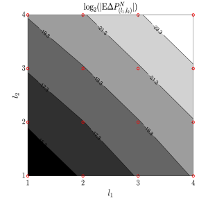
(a)

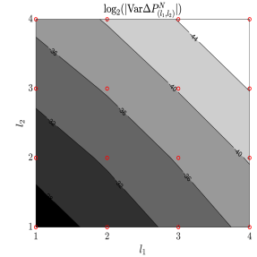
(b)

Figure 1: Contour plots of log values of sample mean and variance of $\Delta P^{N}_{(l_{1}\,l_{2})}$ for $l_{1},l_{2}>0$ used in the sparse combination method.

4.2 Mean and variance of sparse grid increments

Next, we estimate $\mathbb{E}\big{[}\delta P_{l}\big{]}$ and $\mathrm{Var}\big{[}\delta P_{l}\big{]}$, where $\delta P_{l}$ is given by (2.15). From Table 1 we deduce that for the index set $I_{l}=\{(l_{1},l_{2}):l_{1}+l_{2}\leq l+1\}$, the terms on the ‘boundary’ (i.e., $l_{1}=0$ or $l_{2}=0$) will dominate. Although this does not affect the total order of complexity, we can further optimise the cost by modifying the index set such that the contribution from the boundary and ‘interior’ are similar.

Define therefore $\widehat{I}_{l}$ as the indices for interior meshes, and $\widetilde{I}_{l}$ for boundary meshes,

$$\widehat{I}_{l}=\{l_{1}>0,l_{2}>0:l_{1}+l_{2}\leq l\},\quad\widetilde{I}_{l}=\{(l_{1},0):0\leq l_{1}\leq l\}\cup\{(0,l_{2}):0\leq l_{2}\leq l\}.$$

We balance the contributions from these two sets by finding, for some fixed $N$,

$$l^{\ast}\!=\max\bigg{\{}\!\!\operatornamewithlimits{argmin}_{l_{x}\geq 0}\big{|}\mathbb{E}\big{[}\Delta P^{N}_{(1,1)}\big{]}\big{|}/\big{|}\mathbb{E}\big{[}\Delta P^{N}_{(2+l_{x},\,0)}\big{]}\big{|},\ \operatornamewithlimits{argmin}_{l_{y}\geq 0}\big{|}\mathbb{E}\big{[}\Delta P^{N}_{(1,1)}\big{]}\big{|}/\big{|}\mathbb{E}\big{[}\Delta P^{N}_{(0,2+l_{y})}\big{]}\big{|}\!\!\bigg{\}},$$

and using the index set

$$\mathcal{I}_{l}=\begin{cases}\widetilde{I}_{l}&\text{if }l<2+l^{\ast},\\ \widetilde{I}_{l}\cup\widehat{I}_{l-l^{\ast}}&\text{if }l\geq 2+l^{\ast}.\end{cases}$$

For example, from Table 1, $l^{\ast}=2$. So we have

$$\mathcal{I}_{0}=\{(0,0)\},\qquad\mathcal{I}_{l}=\mathcal{I}_{l-1}\cup\{(l,0),(0,l)\},\quad l\in\{1,2,3\},$$

$$\mathcal{I}_{4}=\mathcal{I}_{3}\cup\{(4,0),(0,4),(1,1)\},\qquad\mathcal{I}_{5}=\mathcal{I}_{4}\cup\{(5,0),(0,5),(1,2),(2,1)\},\cdots$$

We use $k_{l}=k_{0}\cdot 2^{-2l}$ and $\mathcal{I}_{l}$ for the construction of $\delta P_{l}$. Table 2 verifies

$$\mathbb{E}[\delta P_{l}]=O(l\,2^{-2l}),\quad\mathrm{Var}[\delta P_{l}]=O(l^{2}\,2^{-4l}),\quad\mathrm{Cost}[\delta P_{l}]=O(l\,2^{3l}).$$

	$l=0$	$l=1$	$l=2$	$l=3$	$l=4$	$l=5$
$\log_{2}\big{|}\mathbb{E}\big{[}\delta P_{l}\big{]}\big{|}$	-0.0647	-7.62	-9.44	-11.42	-13.30	-15.22
$\log_{2}\big{(}\mathrm{Var}\big{[}\delta P_{l}\big{]}\big{)}$	-9.15	-16.93	-20.71	-24.66	-28.20	-31.83
$\log_{2}\big{(}\mathrm{Cost}[\delta P_{l}]\big{)}$	13.64	18.50	22.02	25.22	28.44	31.65

Table 2: Log values of mean, variance, cost for $\delta L_{l}$, $h_{0}=1/2,\ k_{0}=1/8$.

Figure 2 are the corresponding plots. The fitted slopes in Figure 2 are $-1.91,\ -3.73$, and $3.27$, respectively, compared to the theoretical asymptotic values of $-2$, $-4$, and $3$ (neglecting logarithmic terms, which will play a role for low levels).

The cost is counted here as the total number of operations. Specifically, under the ADI scheme (2.3), the cost of one numerical realisation of (1.1) with mesh size $h_{x},\,h_{y}$ and timestep $k$ is

$$\mathrm{cost}/\mathrm{path}\ \sim\ \frac{x_{\text{max}}-x_{\text{min}}}{h_{x}}\cdot\frac{y_{\text{max}}-y_{\text{min}}}{h_{y}}\cdot\frac{T}{k}.$$

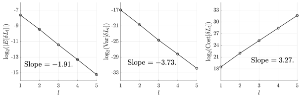
Figure 2: Log values of mean, variance and cost for $\delta P_{l}$.

Since the mean square error for the estimator can be expressed as sum of the variance and the square of the weak error, we split the accuracy “budget” as

$$\big{|}\mathbb{E}\big{[}P_{l}^{N}-P\big{]}\big{|}\leq\alpha\varepsilon,\qquad\mathrm{Var}\big{[}P_{l}^{N}\big{]}\leq(1-\alpha^{2})\varepsilon^{2},$$ (4.1)

and optimize over $\alpha$. Since $V_{l}C_{l}\sim l^{3}\,2^{-l},$ the variance decays with levels more rapidly than the cost increases with levels, and thus the dominant cost is on level $0$. Therefore, we choose $\alpha$ relatively small to reduce the cost on level $0$, and hence we reduce the total cost. To find the optimal $\alpha$, one approach is to approximate the total cost given different $\alpha$, and choose the one which minimise the complexity.

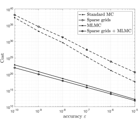
(a) MC, Sparse MC, MLMC, Sparse MLMC.

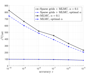
(b) Sparse and full grid MLMC.

Figure 3: Comparison of total cost among different schemes.

Figure 3a is the loglog plot of total cost among all the methods mentioned before: standard Monte Carlo, sparse combination, multilevel Monte Carlo, sparse combination with MLMC. All the schemes use the optimal $\alpha$ for each accuracy. We can see from the graph that standard MC gives the cost $O(\varepsilon^{-4})$, and sparse combination gives $O(\varepsilon^{-7/2})$, as expected. As for MLMC and sparse combination with MLMC methods, both yield approximately $O(\varepsilon^{-2})$, which verifies our proof as the log term in MLMC cost is negligible in this plot.

Figure 3b compares $\varepsilon^{2}W$ between sparse combination with MLMC and MLMC alone (without sparse combination). The total computational cost of sparse combination with MLMC is approximately proportional to $\varepsilon^{-2}$, hence $\varepsilon^{2}W$ does not vary significantly for different accuracy $\varepsilon$. However, as the total cost of the multilevel scheme is proportional to $\varepsilon^{-2}(\log\varepsilon)^{2}$, and we can see from the figure that $\varepsilon^{2}W$ increases as $\varepsilon$ goes to zero. For the black line, we use $\alpha=0.1$. For the blue dotted line, each scheme uses the optimal $\alpha$ for different accuracies. As a result, sparse combination with MLMC achieves the optimal order of complexity.

5 Generalisation to higher dimensions

We can generalise the SPDE to $d$ dimensions, where $d\geq 3$. Let $(\Omega,\mathcal{F},\mathbb{P})$ be a probability space, where there is given a $d$-dimensional standard Brownian motion $W$ with correlation matrix $\Sigma=(\rho_{k,m})$. The natural extension of the SPDE (1.1) is

$$\mathrm{d}v=-\sum_{k=1}^{d}\mu_{k}\frac{\partial v}{\partial x_{k}}\,\mathrm{d}t+\frac{1}{2}\sum_{k,m=1}^{d}\sqrt{\rho_{k}\rho_{m}}\,\rho_{k,m}\frac{\partial^{2}v}{\partial x_{k}\partial x_{m}}\,\mathrm{d}t-\sum_{k=1}^{d}\sqrt{\rho{}_{k}}\frac{\partial v}{\partial x_{k}}\,\mathrm{d}W_{t}^{k},$$ (5.1)

for $x\in\mathbb{R}^{d},\ 0<t\leq T$, where $\mu\in\mathbb{R}^{d}$ and $\rho\in(0,1)^{d}$ are parameters, subject to the Dirac initial datum $v(0,x)=\delta(x_{1}-x_{1,0})\otimes\cdots\otimes\delta(x_{d}-x_{d,0})$, where $x_{0}\in\mathbb{R}_{+}^{d}$ is given.

We use a spatial grid with uniform spacing $h_{x_{i}}>0$, $i=1,\ldots,d$, and let $V_{i_{1},\ldots,i_{d}}^{m}$ be the approximation to $v(mk,i_{1}h_{x_{1}},\ldots,i_{d}h_{x_{d}})$, $m=1,\ldots,N$, $i_{j}\in\mathbb{Z}$, where $i_{0,j}\coloneqq[x_{0,j}/h_{x_{j}}]$, the closest integers to $x_{0,j}/h_{x_{j}}$. We approximate $v(0,x_{1},\ldots,x_{d})$ by

$$V_{i_{1},\dots,i_{d}}^{0}=\prod_{j=1}^{d}h_{x_{j}}^{-1}\delta_{(i_{0,1},\ldots,i_{0,d})}=\begin{cases}\prod_{j=1}^{d}h_{x_{j}}^{-1},\quad&i_{j}=i_{0,j},\quad\forall j\in\{1,\ldots,d\},\\ 0,&\text{otherwise}.\end{cases}$$

In analogy with (1.5), we define a linear functional by

$$P_{T}=\int_{\mathbb{R}_{+}^{d}}v(T,x)\,\mathrm{d}x.$$ (5.2)

Similar as before, we use an implicit finite difference scheme to approximate (5.1), and we use the trapezoidal rule for $P$ with a truncation of the domain. We have the following conjectures and results.

Conjecture 5.1

Assume the implicit finite difference scheme is stable , and the timestep $k$ and mesh size $h_{x_{i}}$ satisfy

$$k\leq\lambda\min\{h_{x_{1}}^{2},h_{x_{2}}^{2},\cdots,h_{x_{d}}^{2}\},$$ (5.3)

for arbitrary fixed $\lambda>0$. Then we have the error expansion

$$\sqrt{\mathbb{E}\big{[}|V_{i_{1},\dots,i_{d}}^{N}-v(T,x_{1},\ldots,x_{d})|^{2}\big{]}}=O(h_{x_{1}}^{2})+O(h_{x_{2}}^{2})+\ldots+O(h_{x_{d}}^{2}),$$

where $N=T/k$ is the number of time steps.

Next we apply the sparse combination method to (5.2) with fixed $k$ satisfying (5.3). Similar to Section 2.2, let $\Delta_{i}$ be the first-order difference operator along directions $i=1,\ldots,d$, defined as in (2.9), and $\Delta=\Delta_{1}\otimes\cdots\otimes\Delta_{d}$.

Conjecture 5.2

Assume the implicit finite difference scheme is stable. Let $h_{x_{i}}=h_{0}\cdot 2^{-l_{i}}$, $i=1,\cdots,d$, and $k$ be the timestep such that for an arbitrary fixed $\lambda>0$, $k\leq\lambda\min\{h_{x_{1}}^{2},h_{x_{2}}^{2},\cdots,h_{x_{d}}^{2}\}$, where $N=T/k$ the number of time steps. Then the first and second moments of $\Delta P^{N}_{\bm{l}}$ satisfy

$$\Big{|}\mathbb{E}\left[\Delta P^{N}_{\bm{l}}\right]\Big{|}=O(h_{x_{1}}^{2}\cdots h_{x_{d}}^{2}),\qquad\mathbb{E}\Big{[}\left|\Delta P^{N}_{\bm{l}}\right|^{2}\Big{]}=O(h_{x_{1}}^{4}\cdots h_{x_{d}}^{4}).$$ (5.4)

Given a sequence of index sets

$$\mathcal{I}_{l}=\{\bm{l}\in\mathbb{N}_{0}^{d}:\,l_{1}+\cdots+l_{d}\leq l+1\},$$

the approximation on level $l$ is defined (similar to (2.12)) as

$${P}_{l}^{N}=\sum_{\bm{l}\in\mathcal{I}_{l}}\Delta P_{\bm{l}}^{N}.$$ (5.5)

Note that we use the same $k$ for all $\Delta P^{N}_{\bm{l}}$, $(l_{1},\cdots,l_{d})\in\mathcal{I}_{l}$. Then we have:

Proposition 5.1

Assume Conjectures 5.1 and 5.2 to be true. Then, for $P$ given by (5.2) and $P_{l}^{N}$ by (5.5), we have

$$\sqrt{\mathbb{E}\left[\lvert P^{N}_{l}-P\rvert^{2}\right]}=O(l^{d-1}\,2^{-2l}).$$

Moreover, by choosing $l=\big{[}\frac{1}{2}(-\log_{2}\varepsilon+(d-1)\log_{2}|\log\varepsilon|)\big{]}$, the computational cost $W$ to achieve a RMSE $\varepsilon$ using standard Monte Carlo estimation is

$$W=O\big{(}\varepsilon^{-\frac{7}{2}}|\log\varepsilon|^{\frac{5}{2}(d-1)}\big{)}.$$ (5.6)

Next, we combine MLMC with the sparse combination scheme. Similar to Section 2.3, let $P_{l}\coloneqq P_{l}^{N_{l}}$ be an approximation to $P$ as in (2.12) using a discretisation with timestep $k_{l}$ and index set $\mathcal{I}_{l}$ defined above. Then we define

$$\delta P_{l}=P_{l}-P_{l-1},\quad l\geq 0,$$ (5.7)

where we denote $P_{-1}\coloneqq 0$. Thus the approximation to $P$ at level $l^{\ast}$ has the form

$$\mathbb{E}[P_{l^{\ast}}]=\sum_{l=0}^{l^{\ast}}\mathbb{E}[\delta P_{l}]=\sum_{l=0}^{l^{\ast}}\mathbb{E}\bigg{[}\sum_{\bm{l}\in\mathcal{I}_{l}}\Delta P_{\bm{l}}^{N_{l}}-\sum_{\bm{l}\in\mathcal{I}_{l-1}}\Delta P_{\bm{l}}^{N_{l-1}}\bigg{]}.$$

In this way, we simulate $\delta P_{l},\,l=0,1,\ldots,l^{\ast}$ instead of directly simulating $P_{l^{\ast}}$, such that the variance of $\delta P_{l}=P_{l}-P_{l-1}$ is considerably reduced by using the same Brownian path for $P_{l}$ and $P_{l-1}$.

Let $\widehat{Y}_{l}$ be an estimator for $\mathbb{E}\big{[}\delta P_{l}\big{]}$ using $M_{l}$ samples. Each estimator is an average of $M_{l}$ independent samples, where $\delta\widehat{P}_{l}^{(m)}$ is the $m$-th sample arising from a single SPDE approximation,

$$\widehat{Y}_{l}=\frac{1}{M_{l}}\sum_{m=1}^{M_{l}}\delta\widehat{P}_{l}^{(m)},\quad l=0,\ldots,l^{\ast}.$$

The MLMC estimator is defined as

$$\widehat{P}_{l^{\ast}}\coloneqq\sum_{l=0}^{l^{\ast}}\widehat{Y}_{l}=\frac{1}{M_{l}}\sum_{m=1}^{M_{l}}\bigg{[}\sum_{\bm{l}\in\mathcal{I}_{l}}\Big{(}\Delta\widehat{P}_{\bm{l}}^{N_{l}}\Big{)}^{(m)}-\sum_{\bm{l}\in\mathcal{I}_{l-1}}\Big{(}\Delta\widehat{P}_{\bm{l}}^{N_{l-1}}\Big{)}^{(m)}\bigg{]},$$ (5.8)

where $\Big{(}\Delta\widehat{P}_{\bm{l}}^{N_{l}}\Big{)}^{(m)}$ is the $m$-th sample for the difference on spatial grid level $\bm{l}=(l_{1},\ldots,l_{d})$ of the SPDE approximation using $N_{l}$ time steps. Following [6], through optimising $M_{l}$ to minimise the computational cost for a fixed variance, we can achieve the optimal complexity $O(\varepsilon^{-2})$ in this case.

Proposition 5.2

Assume Conjectures 5.1 and 5.2 to be true. Given $\delta P_{l}$ from (5.7), there exist $C_{1},\,C_{2},\,C_{3}>0$, such that

$$\mathbb{E}[\delta P_{l}]\leq C_{1}\cdot l^{d-1}\,2^{-2l},\qquad\mathrm{Var}[\delta P_{l}]\leq C_{2}\cdot l^{2d-2}\,2^{-4l},\qquad\mathrm{Cost}[\delta P_{l}]\leq C_{3}\cdot l^{d-1}\,2^{3l}.$$

Then, given a RMSE $\varepsilon$, the MLMC estimator (5.8) leads to a total complexity $O(\varepsilon^{-2})$.

Proof The first inequalities follow directly from (5.4). The complexity then is a small modification of [6, Theorem 3.1]. $\Box$

If we use MLMC without sparse combination to estimate $\mathbb{E}[P_{t}]$, by letting $h_{x_{j}}=h_{0}\cdot 2^{-l}$, $k=k_{0}\cdot 2^{-2l}$, then for constants $C_{1},C_{2},C_{3}>0$, independent of $h$ and $k$,

$$E_{l}\leq C_{1}\cdot 2^{-2l},\quad V_{l}\leq C_{2}\cdot 2^{-4l},\quad W_{l}\leq C_{3}\cdot 2^{(d+2)l}.$$

Similarly, we have the following result.

Proposition 5.3

Given a RMSE $\varepsilon$, the total computational cost $W$ for $P$ in (5.2) using MLMC satisfies

$$W=O\big{(}\varepsilon^{-1-\frac{d}{2}}\big{)},\quad d\geq 3.$$ (5.9)

Comparing (5.9) with (5.6), we can see that when $d>5$, the sparse combination scheme with standard MC performs better than MLMC on regular grids.

6 Conclusion

We considered a two-dimensional parabolic SPDE and a functional of the solution. We analysed the accuracy and complexity of a sparse combination multilevel Monte Carlo estimator, and showed that, by using a semi-implicit Milstein finite difference discretisation (2.2), we achieved the order of complexity $O(\varepsilon^{-2})$ for a RMSE $\varepsilon$, whereas the cost using standard Monte Carlo is $O(\varepsilon^{-4})$, and that using MLMC is $O(\varepsilon^{-2}(\log\varepsilon)^{2})$. When generalising to higher-dimensional problems, sparse combination with MLMC maintains the optimal complexity, whereas MLMC has an increasing total cost as the dimension increases.

Further research will apply this method to a Zakai type SPDE with non-constant coefficients. Another open question is a complete analysis of the numerical approximation of initial-boundary value problems for the considered SPDE.

Appendix A Proofs of some auxiliary stability results

A.1 Proof of Lemma 3.1

Proof For $(\xi,\eta)\in\Omega_{\text{low}}$, we have $G_{(l_{1},\,l_{2})}(\xi,\eta)$ as in (3.11). From (3.5), we have

$$X_{N}^{l_{1},\,l_{2}}-X_{N}^{l_{1},\,l_{2}-1} =X(T)\bigg{(}\exp\big{(}\sum_{n=0}^{N-1}e_{n}^{l_{1},l_{2}}\big{)}-\exp\big{(}\sum_{n=0}^{N-1}e_{n}^{l_{1},l_{2}-1}\big{)}\bigg{)},$$ (A.1)

$$X_{N}^{l_{1},\,l_{2}}-X_{N}^{l_{1}-1,\,l_{2}} =X(T)\bigg{(}\exp\big{(}\sum_{n=0}^{N-1}e_{n}^{l_{1},l_{2}}\big{)}-\exp\big{(}\sum_{n=0}^{N-1}e_{n}^{l_{1}-1,l_{2}}\big{)}\bigg{)},$$

$$X_{N}^{l_{1},\,l_{2}}-X_{N}^{l_{1},\,l_{2}-1}-X_{N}^{l_{1}-1,\,l_{2}}+X_{N}^{l_{1}-1,\,l_{2}-1} =X(T)\bigg{(}\exp\big{(}\sum_{n=0}^{N-1}e_{n}^{l_{1},l_{2}}\big{)}-\exp\big{(}\sum_{n=0}^{N-1}e_{n}^{l_{1},l_{2}-1}\big{)}$$

$$\quad-\exp\big{(}\sum_{n=0}^{N-1}e_{n}^{l_{1}-1,l_{2}}\big{)}+\exp\big{(}\sum_{n=0}^{N-1}e_{n}^{l_{1}-1,l_{2}-1}\big{)}\bigg{)},$$

where

$$X(T)=\exp\bigg{(}-\frac{1}{2}(1-\rho_{x})\xi^{2}T-\frac{1}{2}(1-\rho_{y})\eta^{2}T-\mathrm{i}\xi\sqrt{\rho_{x}k}\sum_{n=0}^{N-1}Z_{n,x}-\mathrm{i}\eta\sqrt{\rho_{y}k}\sum_{n=0}^{N-1}\widetilde{Z}_{n,y}\bigg{)}.$$

By a similar proof to Lemma 4.1 in [19], we have

$$X_{N}^{l_{1},\,l_{2}} =X(T)\cdot R_{0}(T,h_{x}\xi,h_{y}\eta),$$

$$X_{N}^{l_{1},\,l_{2}}-X_{N}^{l_{1},\,l_{2}-1} =O(h_{y}^{2})\cdot X(T)\cdot R_{1}(T,h_{x}\xi,h_{y}\eta),$$

$$X_{N}^{l_{1},\,l_{2}}-X_{N}^{l_{1}-1,\,l_{2}-1} =O(h_{x}^{2})\cdot X(T)\cdot R_{2}(T,h_{x}\xi,h_{y}\eta),$$

$$X_{N}^{l_{1},\,l_{2}}-X_{N}^{l_{1},\,l_{2}-1}-X_{N}^{l_{1}-1,\,l_{2}}+X_{N}^{l_{1}-1,\,l_{2}-1} =O(h_{x}^{2}h_{y}^{2})\cdot X(T)\cdot R_{3}(T,h_{x}\xi,h_{y}\eta).$$

Here, $R_{0},\ R_{1}$, $R_{2}$, $R_{3}$ are random variables satisfying

$$\mathbb{E}\Big{[}\big{|}X(T)\cdot R_{i}(T,h_{x}\xi,h_{y}\eta)\big{|}^{n}\Big{]} =f_{i}(\xi,\eta)\mathrm{e}^{-\frac{n}{2}(\xi^{2}+\eta^{2}+2\xi\eta\sqrt{\rho_{x}\rho_{y}}\rho_{xy})T},\qquad i=0,1,2,3,$$

where $f_{i}(\cdot)$ are polynomial functions. So in the low wave region, we get

$$\quad\mathbb{E}\left[\iint_{\Omega_{\text{low}}}\!\!\!\!G_{(l_{1},\,l_{2})}(\xi,\eta)\,\mathrm{d}\xi\mathrm{d}\eta\right]$$

$$=O(h_{x}^{2}h_{y}^{2})\,\mathbb{E}\bigg{[}\iint_{\Omega_{\text{low}}}\!\!\!4h_{x}h_{y}\chi(2h_{x},\xi)\chi(2h_{y},\eta)\Big{(}X(T)\,R_{3}(T,h_{x}\xi,h_{y}\eta)\Big{)}\mathrm{d}\xi\,\mathrm{d}\eta\bigg{]}$$

$$\quad+O(h_{x}^{2})\,\mathbb{E}\bigg{[}\iint_{\Omega_{\text{low}}}\!\!\!\Big{(}2h_{x}h_{y}\chi(2h_{x},\xi)\chi(h_{y},\eta)-4h_{x}h_{y}\chi(2h_{x},\xi)\chi(2h_{y},\eta)\Big{)}\Big{(}X(T)\,R_{2}(T,h_{x}\xi,h_{y}\eta)\Big{)}\,\mathrm{d}\xi\,\mathrm{d}\eta\bigg{]}$$

$$\quad+O(h_{y}^{2})\,\mathbb{E}\bigg{[}\iint_{\Omega_{\text{low}}}\!\!\!\Big{(}2h_{x}h_{y}\chi(h_{x},\xi)\chi(2h_{y},\eta)-4h_{x}h_{y}\chi(2h_{x},\xi)\chi(2h_{y},\eta)\Big{)}\Big{(}X(T)\,R_{1}(T,h_{x}\xi,h_{y}\eta)\Big{)}\,\mathrm{d}\xi\,\mathrm{d}\eta\bigg{]}$$

$$\qquad\qquad+\mathbb{E}\bigg{[}\iint_{\Omega_{\text{low}}}\!\!\!\Big{(}h_{x}h_{y}\chi(h_{x},\xi)\chi(h_{y},\eta)-2h_{x}h_{y}\chi(h_{x},\xi)\chi(2h_{y},\eta)-2h_{x}h_{y}\chi(2h_{x},\xi)\chi(h_{y},\eta)$$

$$\qquad\qquad\qquad\qquad\qquad+4h_{x}h_{y}\chi(2h_{x},\xi)\chi(2h_{y},\eta)\Big{)}\Big{(}X(T)\,R_{0}(T,h_{x}\xi,h_{y}\eta)\Big{)}\,\mathrm{d}\xi\,\mathrm{d}\eta\bigg{]}.$$

Here,

$$\iint_{\Omega_{\text{low}}}4h_{x}h_{y}\chi(2h_{x},\xi)\chi(2h_{y},\eta)\Big{(}X(T)\cdot R_{3}(T,h_{x}\xi,h_{y}\eta)\Big{)}\,\mathrm{d}\xi\,\mathrm{d}\eta$$

is the numerical approximation to

$$\int_{0}^{\infty}\int_{0}^{\infty}\bigg{(}\iint_{\Omega_{\text{low}}}\mathrm{e}^{\mathrm{i}\xi(x-x_{0})+\mathrm{i}\eta(y-y_{0})}\Big{(}X(T)\cdot R_{3}(T,h_{x}\xi,h_{y}\eta)\Big{)}\,\mathrm{d}\xi\,\mathrm{d}\eta\bigg{)}\,\mathrm{d}x\,\mathrm{d}y$$

by the trapezoidal rule with error $O(h_{x}^{2})+O(h_{y}^{2})$. Therefore,

$$\mathbb{E}\bigg{[}\iint_{\Omega_{\text{low}}}4h_{x}h_{y}\chi(2h_{x},\xi)\chi(2h_{y},\eta)\Big{(}X(T)\cdot R_{3}(T,h_{x}\xi,h_{y}\eta)\Big{)}\,\mathrm{d}\xi\,\mathrm{d}\eta\bigg{]}=O(1).$$

By the same reason,

$$\mathbb{E}\bigg{[}\iint_{\Omega_{\text{low}}}\Big{(}2h_{x}h_{y}\chi(2h_{x},\xi)\chi(h_{y},\eta)-4h_{x}h_{y}\chi(2h_{x},\xi)\chi(2h_{y},\eta)\Big{)}\Big{(}X(T)\cdot R_{2}(T,h_{x}\xi,h_{y}\eta)\Big{)}\,\mathrm{d}\xi\,\mathrm{d}\eta\bigg{]}=O(h_{y}^{2}),$$

$$\mathbb{E}\bigg{[}\iint_{\Omega_{\text{low}}}\Big{(}2h_{x}h_{y}\chi(h_{x},\xi)\chi(2h_{y},\eta)-4h_{x}h_{y}\chi(2h_{x},\xi)\chi(2h_{y},\eta)\Big{)}\Big{(}X(T)\cdot R_{1}(T,h_{x}\xi,h_{y}\eta)\Big{)}\,\mathrm{d}\xi\,\mathrm{d}\eta\bigg{]}=O(h_{x}^{2}),$$

$$\mathbb{E}\bigg{[}\iint_{\Omega_{\text{low}}}\Big{(}h_{x}h_{y}\chi(h_{x},\xi)\chi(h_{y},\eta)-2h_{x}h_{y}\chi(h_{x},\xi)\chi(2h_{y},\eta)-2h_{x}h_{y}\chi(2h_{x},\xi)\chi(h_{y},\eta)$$

$$\qquad\qquad\qquad\qquad\qquad\qquad\qquad\quad+4h_{x}h_{y}\chi(2h_{x},\xi)\chi(2h_{y},\eta)\Big{)}\Big{(}X(T)\cdot R_{0}(T,h_{x}\xi,h_{y}\eta)\Big{)}\,\mathrm{d}\xi\,\mathrm{d}\eta\bigg{]}=O(h_{x}^{2}h_{y}^{2}).$$

Therefore, we get

$$\mathbb{E}\left[\iint_{\Omega_{\text{low}}}\!\!\!\!G_{(l_{1},\,l_{2})}(\xi,\eta)\,\mathrm{d}\xi\mathrm{d}\eta\right]=O\big{(}h_{x}^{2}h_{y}^{2}\big{)}.$$

Similarly,

$$\mathbb{E}\left[\bigg{|}\iint_{\Omega_{\text{low}}}\!\!\!\!G_{(l_{1},\,l_{2})}(\xi,\eta)\,\mathrm{d}\xi\mathrm{d}\eta\bigg{|}^{2}\right]=O\big{(}h_{x}^{4}h_{y}^{4}\big{)}.$$

$\Box$

A.2 Proof of Lemma 3.2

Proof As

$$\Omega_{\text{mid}}=\big{\{}(\xi,\eta):|\xi|\leq h_{x}^{-p}\text{ and }h_{y}^{-p}<|\eta|\leq\pi/h_{y}\big{\}}\cup\big{\{}(\xi,\eta):h_{x}^{-p}<|\xi|\leq\pi/h_{x}\text{ and }|\eta|\leq h_{y}^{-p}\big{\}},$$

it is enough to show for $\Omega_{\text{mid}}^{1}=\{0<|\xi|<h_{x}^{-p},\ h_{y}^{-p}<|\eta|<\pi/h_{y}\}$,

$$\mathbb{E}\Bigg{[}\,\bigg{|}\iint_{\Omega_{\text{mid}}^{1}}\!\!\!\!\!h_{x}h_{y}X_{N}(\xi,\eta)\chi(h_{x},\xi)\chi(h_{y},\eta)\,\mathrm{d}\xi\,\mathrm{d}\eta\bigg{|}^{2}\,\Bigg{]}=o(h_{y}^{r}),$$

We have

$$\mathbb{E}\Bigg{[}\,\bigg{|}\iint_{\Omega_{\text{mid}}^{1}}\!\!\!\!\!h_{x}h_{y}X_{N}(\xi,\eta)\chi(h_{x},\xi) \chi(h_{y},\eta)\,\mathrm{d}\xi\,\mathrm{d}\eta\bigg{|}^{2}\,\Bigg{]}\leq 2\,\mathbb{E}\Bigg{[}\,\bigg{|}\iint_{\Omega_{\text{mid}}^{1}}\!\!\!\!\!h_{x}h_{y}X(T,\xi,\eta)\chi(h_{x},\xi)\chi(h_{y},\eta)\,\mathrm{d}\xi\,\mathrm{d}\eta\bigg{|}^{2}\,\Bigg{]}$$

$$+2\,\mathbb{E}\Bigg{[}\,\bigg{|}\iint_{\Omega_{\text{mid}}^{1}}\!\!\!\!\!h_{x}h_{y}\Big{(}X(T,\xi,\eta)-X_{N}(\xi,\eta)\Big{)}\chi(h_{x},\xi)\chi(h_{y},\eta)\,\mathrm{d}\xi\,\mathrm{d}\eta\bigg{|}^{2}\,\Bigg{]},$$

where $X(T)$ is introduced in (3.2), and $X_{N}$ is given by (3.6). Specifically,

$$X(T) =\prod_{n=0}^{N-1}\exp\Big{(}-\frac{1}{2}(1-\rho_{x})\xi^{2}k-\frac{1}{2}(1-\rho_{y})\eta^{2}k-\mathrm{i}\xi\sqrt{\rho_{x}k}Z_{n,x}-\mathrm{i}\eta\sqrt{\rho_{y}k}\widetilde{Z}_{n,y}\Big{)},$$

$$X_{N} =\prod_{n=0}^{N-1}\frac{1-\mathrm{i}c_{x}\sqrt{\rho_{x}k}Z_{n,x}-\mathrm{i}c_{y}\sqrt{\rho_{y}k}\widetilde{Z}_{n,y}+b_{x}\rho_{x}k(Z_{n,x}^{2}-1)+b_{y}\rho_{y}k(\widetilde{Z}_{n,y}^{2}-1)+d\sqrt{\rho_{x}\rho_{y}}kZ_{n,x}\widetilde{Z}_{n,y}}{1-(a_{x}+a_{y})k}.$$

As $X(T)$ is given in closed form, a direct calculation gives

$$\mathbb{E}\Bigg{[}\,\bigg{|}\iint_{\Omega_{\text{mid}}^{1}}\!\!\!\!\!h_{x}h_{y}X(T,\xi,\eta)\chi(h_{x},\xi)\chi(h_{y},\eta)\,\mathrm{d}\xi\,\mathrm{d}\eta\bigg{|}^{2}\,\Bigg{]}=o(h_{y}^{r}),\quad\forall r>0.$$

Hence, in the following we focus on

$$\mathbb{E}\Bigg{[}\,\bigg{|}\iint_{\Omega_{\text{mid}}^{1}}\!\!\!\!\!h_{x}h_{y}\Big{(}X(T,\xi,\eta)-X_{N}(\xi,\eta)\Big{)}\chi(h_{x},\xi)\chi(h_{y},\eta)\,\mathrm{d}\xi\,\mathrm{d}\eta\bigg{|}^{2}\,\Bigg{]}.$$

Since $h_{x}h_{y}\chi(h_{x},\xi)\chi(h_{y},\eta)$ has finite 2-norm, it is justifiable to consider

$$\mathbb{E}\Bigg{[}\,\bigg{|}\iint_{\Omega_{\text{mid}}^{1}}\!\!\!\!\!X(T,\xi,\eta)-X_{N}(\xi,\eta)\,\mathrm{d}\xi\,\mathrm{d}\eta\bigg{|}^{2}\,\Bigg{]}.$$

First we denote

$$X_{1}(T,\xi)\coloneqq\exp\bigg{(}-\frac{1}{2}(1-\rho_{x})\xi^{2}T-\mathrm{i}\xi\sqrt{\rho_{x}k}\sum_{n=0}^{N-1}Z_{n,x}\bigg{)},\ X_{2}(T,\eta)\coloneqq\exp\bigg{(}-\frac{1}{2}(1-\rho_{y})\eta^{2}T-\mathrm{i}\eta\sqrt{\rho_{y}k}\sum_{n=0}^{N-1}\widetilde{Z}_{n,y}\bigg{)},$$

so that

$$X(T)=X_{1}(T,\xi)X_{2}(T,\eta).$$

Then we introduce $\widetilde{X}_{n}$ such that

$$\widetilde{X}_{N}=\prod_{n=0}^{N-1}\widetilde{C}_{n}^{x}\prod_{n=0}^{N-1}\widetilde{C}_{n}^{y},$$

where

$$\widetilde{C}_{n}^{x}=\frac{1-\mathrm{i}c_{x}\sqrt{\rho_{x}k}Z_{n,x}+b_{x}\rho_{x}k(Z_{n,x}^{2}-1)}{1-a_{x}k},\quad\widetilde{C}_{n}^{y}=\frac{1-\mathrm{i}c_{y}\sqrt{\rho_{y}k}\widetilde{Z}_{n,y}+b_{y}\rho_{y}k(\widetilde{Z}_{n,y}^{2}-1)}{1-a_{y}k}.$$

It has been proved in [18] that

$$X_{1}(T,\xi)-\prod_{n=0}^{N-1}\widetilde{C}_{n}^{x}=X_{1}(T,\xi)\cdot O(h_{x}^{2}),$$

$$\mathbb{E}\bigg{[}\int_{h_{y}^{-p}}^{\pi/h_{y}}\bigg{|}\prod_{n=0}^{N-1}\widetilde{C}_{n}^{y}\bigg{|}^{2}\,\mathrm{d}\eta\bigg{]}=o(h_{y}^{r}),\quad\mathbb{E}\bigg{[}\int_{h_{y}^{-p}}^{\pi/h_{y}}\Big{|}X_{2}(T,\eta)\Big{|}^{2}\,\mathrm{d}\eta\bigg{]}=o(h_{y}^{r}),\qquad\forall r>0.$$

Thus there exists a constant $C$ such that

$$\int_{-h_{x}^{-p}}^{h_{x}^{-p}}\widetilde{X}_{N}-X(T,\xi,\eta)\,\mathrm{d}\xi=C\cdot\big{(}1+O(h_{x}^{2})\big{)}\prod_{n=0}^{N-1}\widetilde{C}_{n}^{y}-C\cdot X_{2}(T,\eta),$$

and as a result,

$$\mathbb{E}\Bigg{[}\,\bigg{|}\iint_{\Omega_{\text{mid}}^{1}}\!\!\!\!\!X(T,\xi,\eta)-\widetilde{X}_{N}(\xi,\eta)\,\mathrm{d}\xi\mathrm{d}\eta\bigg{|}^{2}\,\Bigg{]}\leq\frac{\pi}{h_{y}}\int_{h_{y}^{-p}}^{\pi/h_{y}}\mathbb{E}\bigg{[}\,\bigg{|}\int_{-h_{x}^{-p}}^{h_{x}^{-p}}\!\!\!\!\!X(T,\xi,\eta)-\widetilde{X}_{N}(\xi,\eta)\,\mathrm{d}\xi\bigg{|}^{2}\bigg{]}\mathrm{d}\eta=o(h_{y}^{r}).$$

Since

$$\mathbb{E}\Big{[}\Big{|}X_{n}-\widetilde{X}_{n}\Big{|}^{2}\Big{]}=O(h_{x})\mathbb{E}\big{[}\big{|}\widetilde{X}_{n}\big{|}^{2}\big{]},$$

it follows that

$$\mathbb{E}\bigg{[}\,\bigg{|}\iint_{\Omega_{\text{mid}}^{1}}\widetilde{X}_{N}(\xi,\eta)-X_{N}(\xi,\eta)\,\mathrm{d}\xi\mathrm{d}\eta\bigg{|}^{2}\,\bigg{]} \leq\pi h_{x}^{-p}h_{y}^{-1}\iint_{\Omega_{\text{mid}}^{1}}\mathbb{E}\bigg{[}\Big{|}\widetilde{X}_{N}(\xi,\eta)-X_{N}(\xi,\eta)\Big{|}^{2}\bigg{]}\,\mathrm{d}\xi\mathrm{d}\eta$$

$$=\pi h_{x}^{-p}h_{y}^{-1}\iint_{\Omega_{\text{mid}}^{1}}O(h_{x})\mathbb{E}\Big{[}\big{|}\widetilde{X}_{n}\big{|}^{2}\Big{]}\,\mathrm{d}\xi\mathrm{d}\eta=o(h_{y}^{r}).$$

Therefore,

$$\quad\mathbb{E}\bigg{[}\,\bigg{|}\iint_{\Omega_{\text{mid}}^{1}}\!\!\!\!\!X(T,\xi,\eta)-X_{N}(\xi,\eta)\,\mathrm{d}\xi\mathrm{d}\eta\bigg{|}^{2}\,\bigg{]}$$

$$\leq 2\,\mathbb{E}\bigg{[}\,\bigg{|}\iint_{\Omega_{\text{mid}}^{1}}\!\!\!\!\!X(T,\xi,\eta)-\widetilde{X}_{N}(\xi,\eta)\,\mathrm{d}\xi\mathrm{d}\eta\bigg{|}^{2}\,\Bigg{]}+2\,\mathbb{E}\bigg{[}\,\bigg{|}\iint_{\Omega_{\text{mid}}^{1}}\!\!\!\!\!\widetilde{X}_{N}(T,\xi,\eta)-X_{N}(\xi,\eta)\,\mathrm{d}\xi\mathrm{d}\eta\bigg{|}^{2}\,\bigg{]}=o(h_{y}^{r}).$$

$\Box$

A.3 Proof of Lemma 3.3

Proof For the same reason as in the proof of Lemma 3.2, it is sufficient to prove

$$\mathbb{E}\Bigg{[}\,\bigg{|}\iint_{\Omega_{\text{high}}}X(T,\xi,\eta)-X_{N}(\xi,\eta)\,\mathrm{d}\xi\mathrm{d}\eta\bigg{|}^{2}\,\Bigg{]}=o(h_{x}^{r}h_{y}^{r}).$$

Note that

$$\Omega_{\text{high}}=\big{\{}(\xi,\eta):h_{x}^{-p}<|\xi|\leq\frac{\pi}{2h_{x}}\text{ and }h_{y}^{-p}<|\eta|\leq\frac{\pi}{2h_{y}}\big{\}}.$$

By (3.6), we have

$$X_{N}=X_{0}\prod_{n=0}^{N-1}\frac{1-\mathrm{i}c_{x}\sqrt{\rho_{x}k}Z_{n,x}-\mathrm{i}c_{y}\sqrt{\rho_{y}k}\widetilde{Z}_{n,y}+b_{x}\rho_{x}k(Z_{n,x}^{2}-1)+b_{y}\rho_{y}k(\widetilde{Z}_{n,y}^{2}-1)+d\sqrt{\rho_{x}\rho_{y}}kZ_{n,x}\widetilde{Z}_{n,y}}{1-(a_{x}+a_{y})k}.$$

We denote

$$u=\frac{\sin^{2}\frac{h_{x}\xi}{2}}{(\frac{h_{x}\xi}{2})^{2}}=O(1),\qquad v=\frac{\sin^{2}\frac{h_{y}\eta}{2}}{(\frac{h_{y}\eta}{2})^{2}}=O(1).$$

In this case,

$$\mathbb{E}\big{[}X_{N}\big{]} =X_{0}\prod_{n=0}^{N-1}\mathbb{E}\big{[}C_{n}\big{]}=X_{0}\bigg{(}\frac{1+d\sqrt{\rho_{x}\rho_{y}}\rho_{xy}k}{1+\frac{1}{2}(\xi^{2}u+\eta^{2}v)k}\bigg{)}^{N}$$

$$<X_{0}\exp\bigg{(}-\frac{1}{2}\big{(}\xi^{2}u+\eta^{2}v+2\xi\eta\frac{\sin\xi h_{x}\sin\eta h_{y}}{\xi h_{x}\eta h_{y}}\sqrt{\rho_{x}\rho_{y}}\rho_{xy}\big{)}\,T\bigg{)},$$

$$\mathbb{E}\big{[}\big{|}X_{N}\big{|}^{2}\big{]} =\big{|}X_{0}\big{|}^{2}\prod_{n=0}^{N-1}\mathbb{E}\big{[}\big{|}C_{n}\big{|}^{2}\big{]}$$

$$\leq\big{|}X_{0}\big{|}^{2}\bigg{(}1-\frac{k\xi^{2}u\big{(}1-\rho_{x}\cos^{2}\frac{\xi h_{x}}{2}+\frac{1}{4}\xi^{2}uk(1-2\rho_{x}^{2}(1+2|\rho_{xy}|))\big{)}}{\big{(}1-(a_{x}+a_{y})k\big{)}^{2}}$$

$$\qquad\qquad-\frac{k\eta^{2}v\big{(}1-\rho_{y}\cos^{2}\frac{\eta h_{y}}{2}+\frac{1}{4}\eta^{2}vk(1-2\rho_{y}^{2}(1+2|\rho_{xy}|))\big{)}}{\big{(}1-(a_{x}+a_{y})k\big{)}^{2}}$$

$$\qquad\qquad-\frac{k^{2}\xi^{2}\eta^{2}uv\big{(}1-2\rho_{x}\rho_{y}(1+|\rho_{xy}|+3\rho_{xy}^{2})\big{)}}{2\big{(}1-(a_{x}+a_{y})k\big{)}^{2}}\bigg{)}^{N}$$

$$\leq\big{|}X_{0}\big{|}^{2}\bigg{(}1-\frac{k\xi^{2}u\big{(}\beta+\frac{1}{4}\xi^{2}uk\beta\big{)}}{\big{(}1-(a_{x}+a_{y})k\big{)}^{2}}-\frac{k\eta^{2}v\big{(}\beta+\frac{1}{4}\eta^{2}vk\beta\big{)}}{\big{(}1-(a_{x}+a_{y})k\big{)}^{2}}-\frac{k^{2}\xi^{2}\eta^{2}uv\beta}{2\big{(}1-(a_{x}+a_{y})k\big{)}^{2}}\bigg{)}^{N}$$

$$<\big{|}X_{0}\big{|}^{2}\exp\bigg{(}-\xi^{2}u\beta T\frac{1+\frac{1}{4}\beta\xi^{2}uk}{\big{(}1+\frac{1}{2}(\xi^{2}u+\eta^{2}v)k\big{)}^{2}}-\eta^{2}v\beta T\frac{1+\frac{1}{4}\beta\eta^{2}vk}{\big{(}1+\frac{1}{2}(\xi^{2}u+\eta^{2}v)k\big{)}^{2}}\bigg{)},$$

where

$$\beta=\min\big{\{}1-\rho_{x},1-\rho_{y},1-2\rho_{x}^{2}(1+2|\rho_{xy}|),1-2\rho_{y}^{2}(1+2|\rho_{xy}|),1-2\rho_{x}\rho_{y}(1+2|\rho_{xy}|+3\rho_{xy}^{2})\big{\}}\in(0,1).$$

As we have $k<\lambda\min\{h_{x}^{2},h_{y}^{2}\}$,

$$0<\xi^{2}k<\lambda\pi^{2}/4,\quad 0<\eta^{2}k<\lambda\pi^{2}/4.$$

Also,

$$\min\Big{\{}\frac{u(1+\frac{1}{4}\beta\xi^{2}uk)}{\big{(}1+\frac{1}{2}(\xi^{2}u+\eta^{2}v)k\big{)}^{2}},\frac{v(1+\frac{1}{4}\beta\eta^{2}vk)}{\big{(}1+\frac{1}{2}(\xi^{2}u+\eta^{2}v)k\big{)}^{2}}\Big{\}}>\frac{8}{\pi^{2}\big{(}1+\frac{1}{4}\lambda\pi^{2}\big{)}^{2}}.$$

We define a constant

$$\kappa\coloneqq\frac{8\beta T}{\pi^{2}\big{(}1+\frac{1}{4}\lambda\pi^{2}\big{)}^{2}},$$

then

$$\mathbb{E}\big{[}\big{|}X_{N}\big{|}^{2}\big{]}<|X_{0}|^{2}\exp\big{(}-\kappa\xi^{2}-\kappa\eta^{2}\big{)}.$$

Therefore we have

$$\quad\mathbb{E}\Bigg{[}\,\bigg{|}\iint_{\Omega_{\text{high}}}X_{N}(\xi,\eta)\,\mathrm{d}\xi\mathrm{d}\eta\bigg{|}^{2}\,\Bigg{]}<\frac{\pi^{2}}{h_{x}h_{y}}\iint_{\Omega_{\text{high}}}\mathbb{E}\Big{[}\big{|}X_{N}(\xi,\eta)\big{|}^{2}\Big{]}\,\mathrm{d}\xi\mathrm{d}\eta<\frac{\pi^{2}|X_{0}|^{2}}{h_{x}h_{y}}\iint_{\Omega_{\text{high}}}\mathrm{e}^{-\kappa\xi^{2}-\kappa\eta^{2}}\,\mathrm{d}\xi\mathrm{d}\eta$$

$$=\frac{\pi^{2}|X_{0}|^{2}}{h_{x}h_{y}}\int_{h_{y}^{-p}}^{\pi/h_{y}}\int_{h_{x}^{-p}}^{\pi/h_{x}}\mathrm{e}^{-\kappa\xi^{2}-\kappa\eta^{2}}\,\mathrm{d}\xi\mathrm{d}\eta\leq C\cdot(h_{x}h_{y})^{-1+p}\exp\big{(}-\kappa h_{x}^{-p}-\kappa h_{y}^{-p}\big{)}=o(h_{x}^{r}h_{y}^{r}),\quad\forall r>0.$$

$\Box$

References

- [1] A. Bain and D. Crisan. Fundamentals of Stochastic Filtering, volume 3. Springer, 2009.
- [2] H. Bungartz. Finite elements of higher order on sparse grids. Shaker, 1998.
- [3] H. Bungartz and M. Griebel. Sparse grids. Acta Numer., 13:147–269, 2004.
- [4] N. Bush, B. M. Hambly, H. Haworth, L. Jin, and C. Reisinger. Stochastic evolution equations in portfolio credit modelling. SIAM J. Financ. Math., 2(1):627–664, 2011.
- [5] R. Carter and M. B. Giles. Sharp error estimates for discretizations of the 1d convection–diffusion equation with Dirac initial data. IMA J. Numer. Anal., 27(2):406–425, 2007.
- [6] M. B. Giles. Multilevel Monte Carlo path simulation. Operat. Res., 56(3):607–617, 2008.
- [7] M. B. Giles, F. Y. Kuo, and I. H. Sloan. Combining sparse grids, multilevel MC and QMC for elliptic PDEs with random coefficients. In International Conference on Monte Carlo and Quasi-Monte Carlo Methods in Scientific Computing, pages 265–281. Springer, 2016.
- [8] M. B. Giles and C. Reisinger. Stochastic finite differences and multilevel Monte Carlo for a class of SPDEs in finance. SIAM J. Financ. Math., 3(1):572–592, 2012.
- [9] E. Gobet, G. Pages, H. Pham, and J. Printems. Discretization and simulation of the Zakai equation. SIAM J. Numer. Anal., 44(6):2505–2538, 2006.
- [10] M. Griebel, M. Schneider, and C. Zenger. A combination technique for the solution of sparse grid problems. In P. de Groen and R. Beauwens, editors, Iterative Methods in Linear Algebra, pages 263–281. Elsevier, 1990.
- [11] A. L. Haji-Ali, F. Nobile, and R. Tempone. Multi-index Monte Carlo: when sparsity meets sampling. Numer. Math., 132(4):767–806, 2016.
- [12] C. Hendricks, M. Ehrhardt, and M. Günther. High-order ADI schemes for diffusion equations with mixed derivatives in the combination technique. Appl. Numer. Math., 101:36–52, 2016.
- [13] N. V. Krylov and B. L. Rozovskii. Stochastic evolution equations. J. Sov. Math., 16(4):1233–1277, 1981.
- [14] D. W. Peaceman and H. H. Rachford, Jr. The numerical solution of parabolic and elliptic differential equations. J. Soc. Ind. Appl. Math., 3(1):28–41, 1955.
- [15] C. Pflaum and A. Zhou. Error analysis of the combination technique. Numer. Math., 84(2):327–350, 1999.
- [16] C. Reisinger. Analysis of linear difference schemes in the sparse grid combination technique. IMA J. Numer. Anal., 33(2):544–581, 2012.
- [17] C. Reisinger. Mean-square stability and error analysis of implicit time-stepping schemes for linear parabolic SPDEs with multiplicative Wiener noise in the first derivative. Int. J. Comput. Math., 89(18):2562–2575, 2012.
- [18] C. Reisinger and Z. Wang. Analysis of multi-index Monte Carlo estimators for a Zakai SPDE. J. Comput. Math., 36(2):202–236, 2018.
- [19] C. Reisinger and Z. Wang. Stability and error analysis of an implicit Milstein finite difference scheme for a two-dimensional Zakai SPDE. arXiv preprint arXiv:1802.07682, 2018.
- [20] C. Zenger. Sparse grids. In Parallel Algorithms for Partial Differential Equations: Proceedings of the 6th GAMM-Seminar, Kiel, January 1990, Notes on Numerical Fluid Mechanics 31, W. Hackbusch, ed., Vieweg, Braunschweig, pages 241–251, 1991.