JGraphT - A Java library for graph data structures and algorithms

Abstract

Mathematical software and graph-theoretical algorithmic packages to efficiently model, analyze and query graphs are crucial in an era where large-scale spatial, societal and economic network data are abundantly available. One such package is JGraphT, a programming library which contains very efficient and generic graph data-structures along with a large collection of state-of-the-art algorithms. The library is written in Java with stability, interoperability and performance in mind. A distinctive feature of this library is its ability to model vertices and edges as arbitrary objects, thereby permitting natural representations of many common networks including transportation, social and biological networks. Besides classic graph algorithms such as shortest-paths and spanning-tree algorithms, the library contains numerous advanced algorithms: graph and subgraph isomorphism; matching and flow problems; approximation algorithms for NP-hard problems such as independent set and TSP; and several more exotic algorithms such as Berge graph detection. Due to its versatility and generic design, JGraphT is currently used in large-scale commercial products, as well as non-commercial and academic research projects.
In this work we describe in detail the design and underlying structure of the library, and discuss its most important features and algorithms. A computational study is conducted to evaluate the performance of JGraphT versus a number of similar libraries. Experiments on a large number of graphs over a variety of popular algorithms show that JGraphT is highly competitive with other established libraries such as NetworkX or the BGL.

1 Introduction

Over the last decade, a surge in demand for studying large, complex graphs spurred the development of new packages for graph analysis. Graphs became ubiquitous in every field of study due to their natural ability to capture relationships and interactions between different entities. Graph theoretical problems are regularly encountered in such diverse areas as network security, computational biology, logistics/planning, psychology, chemistry, and linguistics. Despite the vast diversity in graph applications across different fields, their underlying mechanics inevitably rely on the same fundamental mathematical techniques and solution approaches. In keeping with this observation, libraries which efficiently model, store, manipulate and query graphs have become indispensable for engineers and data scientists alike.

This paper introduces JGraphT, a library which contains very efficient and generic graph data-structures along with a sizeable collection of sophisticated algorithms. The library is written in Java, with stability, performance and interoperability in mind. The first version of JGraphT, released in 2003, was primarily intended as a scientific package containing graph-theoretical algorithms. Over the years, JGraphT widened its scope, and added support for algorithms typically encountered in the context of (path) planning, routing, network analysis, combinatorial optimization and applications in computational biology. These developments lead to the adoption of JGraphT into large-scale projects both in academia and industry. As of today, JGraphT is used in a variety of commercial and open-source software packages, including the Apache Cassandra database, the distributed realtime computation system Apache Storm, the Graal JVM, the Constraint Programming Solver Choco, and in Cascading, a software abstraction layer for Apache Hadoop. Similarly, in academia JGraphT has been successfully deployed across a wide range of research domains, including circuit verification [67], malware detection [62], software performance prediction [65], cartography [70], social networking [4], and navigation of autonomous vehicles [30].

Developing a robust, performance-driven, application-independent graph library is a complex task, involving a large number of conflicting (functional and structural) design choices and performance trade-offs. In this paper, we formally outline the design of JGraphT, and highlight several of its design considerations. Moreover, we provide an overview of the most important features and algorithms currently supported by JGraphT. Among others, this overview covers routing algorithms such as shortest path algorithms or advanced heuristics for A*; network analysis with clustering coefficients and centrality metrics; network optimization and matching problems; min-cut and max-flow algorithms; graph mining with graph kernels; and subgraph isomorphism detection. To show JGraphT’s competitiveness, we perform a computational comparison with other well-established graph libraries.

The remainder of this paper is structured as follows. Section 2 discusses related work and alternative graph libraries. Next, Section 3 describes JGraphT, its components and its internal design in detail. An overview of the various algorithms supported by JGraphT is provided in Section 4, followed by an overview of graph generators in Section 5. To provide interoperability between different mathematical packages, JGraphT natively supports a large variety of graph formats, summarized in Section 6. An extensive computational study—covering an external comparison of algorithms from different libraries, an internal comparison of alternative algorithms for the same mathematical problems, and a comparison of different graph representations—is presented in Section 7. Finally, Section 8 concludes the paper.

2 Related Work

Software solutions for graph theory exist in many forms. On one side of the spectrum, there are the mathematical ecosystems such as Wolfram Mathematica [58], Sage Math [100] and Maple [69] which provide high-level functions to model, analyze and visualize graphs and networks. On the other side, there are graph theoretical libraries and algorithmic packages such as JGraphT, which are primarily designed to aid software development. From a scientific point of view, the two best-known libraries are LEDA [76] and the Boost Graph Library [92] (BGL), which are both written in C$\mathrel{++}$. LEDA offers a very efficient graph data-structure, along with some of the most efficient implementations of classic graph algorithms. BGL, on the other hand, follows a generic programming paradigm in order to provide highly optimized graph algorithms.

Despite the popularity of Java as a programming language in academia and industry, the number of graph packages written in Java is very limited. Currently, there exist only two viable alternatives to JGraphT: the Java Universal Network/Graph Framework (JUNG) library [81] and a graph component in the Google Guava library. JUNG provides a graph data-structure, several basic algorithms such as shortest paths and centrality metrics, and a graph drawing (layout) component. Google Guava, on the other hand, currently only contains a number of graph data structures, including ’Graph’, ’ValueGraph’ and ’Network’. Out of these three, ’Network’ is the most general one and corresponds almost one-to-one with the JGraphT graph interface. To provide algorithmic support for Guava, JGraphT contains adapter classes which allow users to invoke all algorithms in JGraphT on Guava graph data-structures.

Software packages for network analysis can be broadly categorized as: (1) packages for data structures and storage, including databases for large-scale networks; (2) algorithmic packages for network analysis, primarily meant to create insights into the network data; and (3) packages for graph visualizations to generate meaningful, human-interpretable, visual representations. Of particular interest to us are the packages that fall within the second category. The igraph [25] library, written in C, contains several optimized algorithms for network analysis. igraph is designed to handle large graphs efficiently and to be easily embeddable in higher level programming languages such as Python and R. NetworkX [52] is a Python library designed to study the structure and dynamics of complex networks. It contains data structures for graphs, digraphs and multigraphs, as well as many standard graph and network analysis algorithms. Moreover, similar to JGraphT, NetworkX is platform independent. NetworKit [93] is yet another open-source package for large-scale network analysis. It is written in C++, employing parallelization when appropriate, and provides Python bindings for ease-of-use. The Stanford Network Analysis Platform (SNAP) [66] is a general-purpose, high-performance system that provides easy-to-use, high-level operations for analysis and manipulation of large networks. The library focuses on single big-memory machines and provides a large collection of graph algorithms including dynamic algorithms. Similarly to the other libraries, it is written in C++ with Python bindings.

Next to the traditional graph libraries, there exist a number of specialized libraries designed for large-scale, parallel computing applications. These libraries typically implement frameworks that rely on distributed computing (Parallel Boost Graph Library [49], Distributed GraphLab [68]), multi-core CPU (Ligra [91], GraphMat [95]), or GPU architectures (GraphBLAST [105], Gunrock [103], nvgraph) to execute graph operations on massive graphs in parallel. Several of these frameworks, including GraphMat, GraphBLAS [61] and GraphBLAST, represent graphs through sparse adjancency matrices, and use matrix algebra to implement graph operations. These frameworks are, among others, particularly suited for implementing parallel graph traversal algorithms such as Breadth-First-Search, Pagerank and single-source shortest paths. Empirical studies and comparisons of a number of these libraries have been published in [88, 50]. Additionally, a community effort has been launched [73] in order to implement more graph algorithms using the GraphBLAS API.

Finally, there exist a large number of software packages and libraries that focus on graph visualization such as Gephi [7], Cytoscape [89], and GraphViz [35]. While it is possible to couple JGraphT with visualization libraries, the library currently does not offer drawing capabilities by itself.

3 Design

JGraphT is designed with a strong focus on flexibility, versatility and performance. This section outlines the design of JGraphT and discusses trade-offs and considerations encountered in the design of the library.

3.1 The Graph interface

JGraphT is built around a central fig:jgraphtuml). This interface provides elementary operations for the construction of a graph, as well as basic operators to access elements of the graph (Figure 2). All interactions with the graph occur through this interface: every predefined graph class in the library implements this interface, and all of JGraphT’s algorithms expect a ¡V¿ and permits the user to use any type of object as edge or vertex. In its simplest form, the vertices of a graph are represented by Integers or Strings, while the edges are represented by a default edge implementation called Intersection class which stores the geographical coordinates of an intersection, as well as a extremely versatile, as its basic data structures are capable of capturing and expressing any type of relationship or interaction between any type of object in a natural way. JGraphT provides implementations of common graph types such as simple graphs, multigraphs, pseudographs, etc. Each of these graph types can be refined as directed or undirected, and weighted or unweighted. An overview of predefined graph types can be found in Table 1. Since each graph implements the aforementioned degreeOf(V vertex), for instance, returns the number of edges touching a vertex (with self-loops counted twice) in case of an undirected graph, whereas the same method returns the sum of the in-degree and the out-degree in case of a directed graph. Similarly, the mintedjava Graph¡Integer, DefaultEdge¿ graph = new SimpleGraph¡¿(DefaultEdge.class); Choosing a particular graph implementation, however, can be non-trivial for users foreign to graph theoretical concepts. One potential strategy to circumvent this issue is to select the most general graph implementation by default. For instance, a pseudograph which supports multiple edges and self-loops can be used to represent a simple graph which does not support these features. This however comes with a clear performance penalty, since pseudographs typically take more space, and operations on these graphs take more time than their more specialized counterparts. To circumvent this issue, and to simplify the process of selecting the desired type of graph, JGraphT allows the user to construct graphs through a builder pattern [42] after which the library automatically determines the most suitable graph implementation:

⬇

Graph<Integer, DefaultEdge> graph =

GraphTypeBuilder.<Integer, DefaultEdge> directed()

.allowingMultipleEdges(true)

.allowingSelfLoops(false).

.edgeClass(DefaultEdge.class)

.buildGraph();

Algorithms which behave differently depending on the underlying graph characteristics, can query the graph during runtime for its GraphType}. The \mintinlineJavaGraphType contains the necessary type information, defining whether the graph is directed or undirected, weighted or unweighted, and whether it allows self-loops, multiple-edges, etc.

3.2 Graph structure

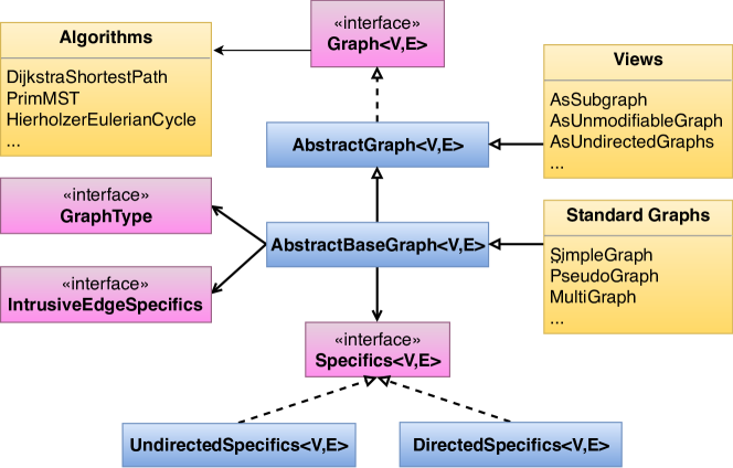
Figure 1: Core structure of JGraphT

The structural design of JGraphT, as depicted in Figure 1, separates the functional JavaAbstractGraph offers a minimal implementation of this Graph interface, without explicitly defining the data structures for storage and indexing as these are managed by the graph backend. The graph backend extends AbstractGraph}, records the \mintinlineJavaGraphType, and implements data structures to physically store the graph. Figure 1 depicts the default backend, implemented by the AbstractBaseGraph} class. Most of the predefined graph classes listed in Table~\reftable:graphclasses are subclasses of the AbstractBaseGraph} class. A detailed discussion of the different graph backends supported by \jgrapht is provided in Section 3.3. To implement a new graph type, or to adjust the underlying implementation of an existing graph type, the user would typically instantiate, override or extend some of the classes depicted in Figure 1. Views over graphs, for instance, can be defined by extending AbstractGraph}. This is similar to the concept of filtered graphs in \bgl. All operations invoked on a view are delegated to the graph backing the view. Consequently, views offer a natural way to model, for instance, induced subgraphs (

AsSubgraph}). They can
also be used to treat a directed graph as an undirected graph (\mintinline

JavaAsUndirectedGraph), to add weights to an unweighted graph (AsWeightedGraph}) or to render a graph unmodifiable (\mintinlineJavaAsUnModifiableGraph). In addition to views, it is possible to define adapter classes by extending

AbstractGraph}. One
such example can be found in the \verb|jgrapht-guava| package, which implements adapters for graph-data structures encountered
in the Guava Library\footnote

https://github.com/google/guava. Through these adapters, a user can invoke all algorithms described in Section 4 on graphs implemented with Guava data-structures.

3.3 Graph backends

The underlying implementation and data storage of a graph, independent of whether the graph type is predefined or user-defined, is highly customizable. There exist many scenarios where domain specific knowledge of the end-user is required to determine the best choice of data structures. Particularly relevant in this context are: type of data being represented; graph density (sparse or dense graph); graph size (number of edges/vertices); available storage space; performance requirements; and the type of graph operations that will be most frequently performed. Similar considerations are made when explicitly storing an adjacency matrix to lookup adjacent vertices (neighbors) or when selecting the structures used to represent the incidence matrix. If for instance the vertices are simple integers, the incidence matrix can be a 2-dimensional array, whereas in case of arbitrary vertex objects we must resort to hash tables. Fine-grained control over how the data in a graph is stored can be obtained by adjusting the graph backend. JGraphT provides two predefined backends which collectively cover most common use-cases: the default backend and the sparse backend. In addition, the user can implement custom backends, simply by creating a new subclass of the AbstractGraph} class (Figure~\reffig:jgraphtuml). It is worth noting that when using the predefined backends, all operations invoked on JGraphT graphs are performed in a deterministic fashion. This behavior is realized through the usage of data structures having a predictable iteration order such as lists, as well as sets and maps backed by doubly linked lists (LinkedHashSet} and \mintinlineJavaLinkedHashMap). The default backend, implemented by the AbstractBaseGraph} class (Figure~\reffig:jgraphtuml), is designed to offer a good trade-off between performance and memory consumption. Since vertices and edges can be modeled by arbitrary objects, the default backend primarily relies on hash tables to store vertices and edges, and to implement adjacency lists. Consequently, basic operations such as vertex or edge removal and addition can be performed in expected constant ($\mathcal{O}(1)$) time. An (optional) indexing mechanism is provided to index edges by their two endpoints to enable fast edge lookups. This indexing mechanism again provides a trade-off between performance and additional memory consumption. The user can further customize how the adjacency and incidence matrices are stored and how edge lookups are performed (including how edge weights are stored) by providing alternative implementations of the Specifics} and \mintinlineJavaIntrusiveEdgesSpecifics interfaces. For instance, the standard Java hash tables used to store the adjacency and incidence matrices can be swapped out by specialized alternatives from the Fastutil library or from the Eclipse Collections to reduce the memory footprint of a graph. The default backend is well-suited for general-purpose graphs which efficiently support edit operations such as the addition or removal of a single vertex or edge. Better performance, however, can be achieved in a less dynamic setting where the graph is constructed in a single bulk operation. Such a write-once read-many strategy is very common when executing complex algorithms on graphs, which usually involve loading a graph from an external source into memory, executing the algorithms, and querying the final result. To accommodate such a use-case, JGraphT provides a specialized sparse graph backend which implements the

Graph<Integer,Integer>} interface and hence requires that all vertices and edges
are represented by integers. Here it is assumed that the vertices are numbered $0, \ldots, n-1$
while edges are numbered $0, \ldots, m-1$, where $n$ and $m$ are resp.\ the number of vertices and
edges in the graph. The latter assumption renders edit operations less efficient, since adding or
removing a vertex (resp.\ edge) potentially involves re-numbering all other vertices and edges.
To reduce the storage space requirements of a graph, the sparse backend stores the incidence
matrix in Compressed-Sparse-Rows (CSR) format~\cite

saad2003iterative, thereby taking advantage of the fact that most real-world graphs are sparse graphs. Graphs stored in this format support both self-loops and multiple-edges. An overview of the sparse graphs and their capabilities is provided in Table 1. To implement undirected graphs, the sparse backend represents the incidence matrix through a single boolean matrix, whereas two boolean matrices (one for each direction) are used for directed graphs. Edge weights, in case of weighted graphs, are stored in a simple array of length $m$.

⬇

public interface Graph<V,E> {

GraphType getType();

\parV addVertex();

boolean removeVertex(V v);

E addEdge(V sourceVertex, V targetVertex);

boolean removeEdge(E e);

\parSet<V> vertexSet();

Set<E> edgeSet();

\parV getEdgeSource(E e);

V getEdgeTarget(E e);

E getEdge(V sourceVertex, V targetVertex);

\pardouble getEdgeWeight(E e);

void setEdgeWeight(E e, double weight);

\parSet<E> edgesOf(V v);

\par/* More methods omitted */

}

Figure 2: The Graph¡V,E¿— interface. All interactions with the graph happen through this interface.

class name	edges	self-loops	multiple-edges	weighted
SimpleGraph	undirected	✗	✗	✗
Multigraph	undirected	✗	✓	✗
Pseudograph	undirected	✓	✓	✗
DefaultUndirectedGraph	undirected	✓	✗	✗
SimpleWeightedGraph	undirected	✗	✗	✓
WeightedMultigraph	undirected	✗	✓	✓
WeightedPseudograph	undirected	✓	✓	✓
DefaultUndirectedWeightedGraph	undirected	✓	✗	✓
SparseIntUndirectedGraph	undirected	✓	✓	✗
SparseIntUndirectedWeightedGraph	undirected	✓	✓	✓
SimpleDirectedGraph	directed	✗	✗	✗
DirectedMultigraph	directed	✗	✓	✗
DirectedPseudograph	directed	✓	✓	✗
DefaultDirectedGraph	directed	✓	✗	✗
SimpleDirectedWeightedGraph	directed	✗	✗	✓
DirectedWeightedMultigraph	directed	✗	✓	✓
DirectedWeightedPseudograph	directed	✓	✓	✓
DefaultDirectedWeightedGraph	directed	✓	✗	✓
SparseIntDirectedGraph	directed	✓	✓	✗
SparseIntDirectedWeightedGraph	directed	✓	✓	✓

Table 1: All available graph implementation classes.

4 Algorithms

JGraphT contains a large number of algorithms. A detailed discussion of each algorithm is outside the scope of this paper; instead a general overview of the algorithms currently supported is provided. Most of these algorithms are single-threaded, unless otherwise explicitly mentioned.

Connectivity

Detecting connected components in graphs is a fundamental problem. For undirected graphs or weakly connected components in directed graphs, standard traversals such as BFS or DFS suffice. For directed graphs, the library provides the linear time algorithm of Kosaraju-Sharir [90] using two DFS traversals, as well as Gabow’s algorithm [40]. The classic Algorithm 447 [56] is also provided for the computation of biconnected components. These algorithms can also be used to identify cutpoints and bridges in a graph, or to construct a Block-Cutpoint graph.

LCA

The least common ancestor of two nodes $v$ and $u$ in a tree or in a directed acyclic graph (DAG) $T$, is the deepest node that has both $v$ and $u$ as descendants. A naive implementation (supporting both trees and DAGs) and the offine tree algorithm of Tarjan [41] can be used for small graph sizes or for batched queries. For larger tree instances, the library provides three additional implementations with different space time tradeoffs: (a) using the heavy-path decomposition with linear space to support LCA queries in $\mathcal{O}(\log n)$ time, (b) using the Euler-Tour technique [12] and the classic reduction [9] to the RMQ (range minimum query) problem to support LCA queries in $\mathcal{O}(1)$ time but with $\mathcal{O}(n\log n)$ space, and (c) a preprocessing approach which improves over the naive approach by computing jump pointers, using dynamic programming [10]. In the latter approach, each node stores jump pointers to ancestors at levels $1,2,4,\ldots,2^{k}$. Queries are answered by repeatedly jumping from node to node, each time jumping more than half of the remaining levels between the current ancestor and the goal ancestor (i.e. the lca). The worst-case number of jumps is $\mathcal{O}(\log n)$ which means that this method has $\mathcal{O}(\log n)$ query time again using $\mathcal{O}(n\log n)$ space.

Cycles

Another fundamental problem involves enumerating all simple cycles of a graph. Several classic algorithms have been implemented for this problem such as the algorithms of Tiernan [101], Tarjan [99], Johnson [60], Szwarcfiter and Lauer [97], and Hawick and James [53]. Additionally, the set of Eulerian subgraphs (subgraphs where all vertices have even degrees) forms the cycle space of a graph (over the two-element finite field). A cycle basis is a basis of this vector space. The library contains a variant of Paton’s algorithm [85] as well as some classic fundamental cycle basis construction algorithms using graph traversals [27].

Shortest Paths

The library contains extensive support for shortest path computations, both single-source and all-pairs. When all edge weights are non-negative, Dijkstra’s algorithm can be used. In JGraphT, Dijkstra’s algorithm is implemented using a Fibonacci heap. A bidirectional variant is also included which enhances performance significantly for source-target queries. Additionally, when edge weights can be negative, users can resort to the Bellman-Ford algorithm or Johnson’s algorithm. Support for all-pairs shortest paths is provided by the Floyd-Warshall algorithm. The delta-stepping algorithm [77], a parallel algorithm for the single-source shortest path problem, is also included. The library also contains an A* implementation together with the ALT admissible heuristic [45] and Martin’s algorithm for the multi-objective shortest paths problem [71]. With respect to $k$-shortest paths, JGraphT includes variants of the Bellman-Ford algorithms for finding $k$-shortest simple paths, Eppstein’s algorithm [36] for finding the $k$ shortest paths between two vertices, Yen’s [72] algorithm for finding loop-less shortest paths and Suurballe and Tarjan [96] algorithm for finding edge disjoint shortest paths. Finally, a graph measurer class offers additional distance related metrics such as the graph diameter, the radius, vertex eccentricities, the graph center, and graph (pseudo) periphery.

Node Centrality

Node centrality measures the importance of nodes inside a network. Centrality metrics play a crucial role in social network analysis. The library support several vertex centrality [79] metrics including alpha, betweenness, closeness, coreness, harmonic centrality and PageRank; see [78] for details. For betweenness centrality the algorithm of Brandes [15] is used. Coreness is computed using the techniques described in [74]. The remaining measures are computed using power iteration.

Spanning Trees and Spanners

The minimum spanning tree problem asks to compute a spanning tree in a weighted graph of minimum total weight. The library includes Prim, Kruskal and Borůvka’s algorithms for the construction of minimum spanning trees. Prim’s algorithm is implemented with a Fibonacci heap, while Kruskal’s and Borůvka’s algorithms rely on a Union-Find data structure with union-by-rank and path-compression. More general spanners can also be computed using for example the greedy algorithm for $(2k-1)$-multiplicative spanner construction [3].

Recognizing Graphs

The library contains algorithms for the recognition of important types of graphs. Examples are bipartite graphs, chordal graphs and Berge graphs. Bipartite graphs are recognized by standard graph traversals. For the recognition of chordal graphs we compute a perfect elimination order either using maximum cardinality search [13] or lexicographic breadth first search [24]. Both require linear time. Finally, recognizing Berge graphs is accomplished using the $\mathcal{O}(n^{9})$ state-of-the-art algorithm of Chudnovsky et al. [20]. Recall that a graph is Berge if no induced subgraph of $G$ is an odd cycle of length at least five or the complement of such a cycle.

Matchings

Matching algorithms for general, bipartite, weighted and unweighted graphs are provided. For maximum cardinality matching in general graphs the library includes the highly efficient $\mathcal{O}(mn\alpha(m,n))$ implementation of Edmonds [31] algorithm presented in the LEDA book [76]. For bipartite graphs, the user can invoke Hopcroft and Karp’s algorithm [57]. To calculate a maximum weight matching in bipartite graphs, there is a highly efficient $\mathcal{O}(n(m+n\log n))$ implementation, again from the LEDA book. Minimum weight perfect bipartite matchings can be computed using the $\mathcal{O}(n^{3})$ Hungarian method. To compute a minimum weight perfect matching in general graphs, there is an efficient implementation of Edmond’s algorithm using the techniques introduced by the Blossom V implementation [64]. Finally, several fast $1/2$-approximation algorithms for matchings are provided, including (a) a greedy algorithm and (b) the linear time path growing [29] algorithm.

Cuts and Flows

Maximum flows and minimum cuts in graphs are by definition closely related. The maximum flow problem [1] involves calculating a feasible flow of maximum value from a source vertex $s$ to a sink vertex $t$ through a capacitated network. Similarly, a minimum $s-t$ cut in a graph is a partitioning of the vertices $V$ into two disjoint subsets $S$ and $T$ such that $s\in S$, $t\in T$ while minimizing the sum of weights of the edges with exactly one endpoint in $S$ and one endpoint in $T$. To efficiently calculate maximum $s-t$ flows, and by extension minimum $s-t$ cuts, the library provides implementations of the Edmonds-Karp algorithm [33], the Push-Relabel algorithm [46], and Dinic’s algorithm [28]. Determining maximum $s-t$ flows or minimum $s-t$ cuts for every $s-t$ pair in the graph can be realized by computing resp. an Equivalent Flow tree [51] or a Gomory-Hu tree [48] using Gusfield’s algorithm. The Gomory-Hu tree can also be used to compute the minimum cut in the graph, i.e. the minimum cut over all $s-t$ pairs. Alternatively, the user can employ Stoer and Wagner’s algorithm [94] for this purpose. Finally, the more general minimum-cost flow problem, which considers both costs and capacities for each arc in the network, can be solved by the successive shortest path algorithm, with or without capacity scaling [1]. An implementation of the algorithm by Padberg and Rao [82] to compute Odd Minimum Cut-Sets is also present.

Isomorphism

(Sub)graph isomorphisms can be computed through the classic VF2 [23] algorithm. Additionally, efficient heuristic isomorphic tests based on color refinement [11] are also provided.

Coloring

The well-know NP-hard graph coloring problem entails the assignment of colors to vertices of a graph such that no two adjacent vertices share the same color. The library includes the exact coloring algorithm of Brown [17] as well as several heuristic algorithms such as (a) greedy, (b) random greedy, (c) largest-degree-first (d) smallest-degree-last, and (e) saturation-degree [16] coloring.

Cliques

The Bron-Kerbosch algorithm is an algorithm for enumerating all maximal cliques in an undirected graph. The library contains several variants.

• Implementation of the Bron-Kerbosch clique enumeration algorithm as described in [87].

• Bron-Kerbosch maximal clique enumeration algorithm with pivot. The pivoting follows the rule from Tomita et al. [102], in which the authors show that this rule guarantees that the Bron-Kerbosch algorithm has worst-case running time $\mathcal{O}(3^{n/3})$, excluding time to write the output, where $n$ is the number of vertices of the graph; this is worst-case optimal.

• Bron-Kerbosch maximal clique enumeration algorithm with pivot and degeneracy ordering. The algorithm is a variant of the Bron-Kerbosch algorithm which apart from the pivoting uses a degeneracy ordering of the vertices. The algorithm is described in Eppstein et al. [37] and has running time $\mathcal{O}(dn3^{d/3})$ where $n$ is the number of vertices of the graph and $d$ is the degeneracy of the graph.

Moreover, algorithms to compute clique minimal separator decompositions [14] and maximum cliques in chordal graphs are also provided.

Vertex Cover

The minimum vertex cover problem is yet another classical NP-hard problem and involves selecting a subset of vertices of minimum cardinality such that each edge of the graph is incident to at least one selected vertex. JGraphT provides (a) an exact branch-and-bound algorithm, (b) a greedy heuristic and (c) various 2-approximation algorithms which differ either in running time or in solution quality, including the Bar-Yehuda and Even algorithm [5] and Clarkson’s algorithm [22].

Tours

Several algorithms to compute tours, that is, both Hamiltonian Cycles (HCs) and Eulerian Cycles (ECs), are available. To solve the Traveling Salesman Problem (TSP) with optimality, thereby obtaining a minimum cost HC, the Held-Karp dynamic programming algorithm can be used. For weighted graphs satisfying the triangle inequality, two approximation algorithms are provided. The first algorithm is a 2-approximation and follows a traditional approach which first computes a MST, which is then traversed in a depth-first search manner to obtain a tour. The second algorithm is an implementation of Christofides $3/2$-approximation [19]. Finally a 2-OPT heuristic is available to quickly compute HCs, but without any quality guarantees. Determining whether a graph permits any HC irrespective of its cost remains an NP-Complete problem. Nevertheless, whenever the input graph satisfies Ore’s condition, a HC can be identified in polynomial time ($\mathcal{O}(|V|^{2})$) using Palmer’s algorithm [83]. Ore’s condition essentially states that a graph with sufficiently many edges must contain a HC. In addition to HCs, it is also possible to calculate ECs. ECs play an important role in the context of Arc Routing. To find an EC in Eulerian graphs, Hierholzer’s algorithm [54] can be used. Similarly, the Chinese Postman Problem, requiring the calculation of a tour (closed walk) of minimum length which traverses every edge in a graph at least once, can be solved efficiently using an implementation of Edmond’s algorithm [32]. Obviously, when the input graph is Eulerian, Edmond’s algorithm returns an EC; otherwise the algorithm returns a closed walk of minimum length which traverses some edges multiple times.

5 Generators

JGraphT provides a number of graph generators to deterministically generate graphs of arbitrary size which model and capture characteristics of real-world networks, e.g. social networks, communication networks, chemical interactions etc. These generators enable engineers and researchers to generate arbitrarily large synthetic datasets resembling real world data, without the need to go through a costly and often time-consuming data collection process. Various types of graphs can be generated, including: complete graphs, bipartite graphs, grid graphs, hypercubes, ring graphs, star graphs, wheel graphs, and others. Additionally, dedicated generators for specific graphs famous in Graph Theory such as the Doyle graph, the Petersen graph, Balaban graphs, etc are also provided. Random graphs can be generated through the traditional $Gnm$ and $Gnp$ Erdös-Rényi [38] models. In the $Gnm$ model, a graph is chosen uniformly at random from the set of all graphs with $n$ nodes and $m$ edges. In the $Gnp$ model a graph of $n$ nodes is constructed and each of the possible edges is chosen with probability $p$. Similar models are available for the generation of random bipartite graphs where the user specifies the size of the two partitions and either the number of edges or the edge probability. Finally, generators for random regular graphs are also available. More sophisticated models popular in e.g. social sciences are also provided. The Barabási-Albert [6] model starts from a small clique and incrementally constructs a graph by adding new vertices one by one. Each new vertex is attached to a certain number of previously constructed vertices using preferential attachment. The Watts-Strogatz [2] model builds a graph by interpolating between a regular lattice and a random graph. It starts from a regular lattice with $n$ nodes and $k\ll n$ edges per node. Then it chooses a vertex and the edge that connects it to its nearest neighbor in a clockwise sense. With probability $p$, it reconnects this edge to a vertex chosen uniformly at random over the entire ring with duplicate edges forbidden; otherwise it leaves the edge in place. It continues this process for each vertex of the ring and then repeats the procedure for the second-nearest neighbor, etc. As there are $\frac{nk}{2}$ edges in the entire graph, the rewiring process stops after $\frac{k}{2}$ laps. For intermediate values of $p$, the graph is a small-world network: highly clustered like a regular graph, yet with small characteristic path length, like a random graph. A small variant [80] is also provided wherein instead of re-wiring, the shortcut edges are added to the graph. This variant is sometimes called the Newman-Watts variant of the Watts-Strogatz model. The Kleinberg [63] small-world model, which is also implemented, has as a basic structure a two-dimensional grid and allows for edges to be directed. It begins with a set of nodes (representing individuals in the social network) that are identified with the set of lattice points in an $n\times n$ square. For a universal constant $p\geq 1$, the node $u$ has a directed edge to every other node within lattice distance $p$ (these are its local contacts). For universal constants $q\geq 0$ and $r\geq 0$, we also construct directed edges from $u$ to $q$ other nodes (the long-range contacts) using independent random trials; the i-th directed edge from $u$ has endpoint $v$ with probability proportional to $\frac{1}{d(u,v)^{r}}$ where $d(u,v)$ is the lattice distance from $u$ to $v$.

6 Importing & Exporting Graphs

To increase interoperability between JGraphT and other software solutions, and to facilitate efficient storage of graphs, JGraphT enables the user to read and write graphs in a variety of popular data formats. Some of the common formats are: GML [55], CSV, DIMACS [59], graph6 and sparse6 [75]. In particular, for DIMACS the library supports the formats used in the 2nd challenge for max-clique problems and graph coloring problems, as well as the shortest path format used in the 9th challenge. Sparse6 and graph6 are formats used for storing graphs in a compressed manner, using printable ASCII characters only. Besides the aforementioned formats, JGraphT also supports richer formats capable of storing additional information such as graph attributes and labels. Among these formats are the DOT language specification [43] and GraphML [98]. Both formats are fully supported. The implementations rely on Antlr v4 [84] for low-level parsing. For GraphML, two parsers are provided: one light-weight parser optimized towards parsing speed, and one full fledged parser which implements the complete GraphML specifications.

7 Experimental Evaluation

This section provides a computational evaluation of JGraphT. In the evaluation, various algorithms from JGraphT (v1.4) are compared against their counterparts in alternative graph libraries. Given the large number of different algorithms and libraries, it is by no means possible to provide an exhaustive comparison. Therefore, a number of commonly used algorithms and libraries have been selected. These libraries were selected because of their popularity, plus the fact that they are open-source, actively maintained and developed, and supporting a wide range of algorithms. In particular, comparisons are made against igraph (v0.7.1 written in C), BGL (v1.65 written in C++), Jung (v2.1.1 written in Java) and NetworkX (v2.1 written in Python). The igraph library represents graphs using a simple compressed-sparse-rows (CSR) based representation, which requires six different vectors, two of size $n$ and four with size $m$. BGL, on the other hand, implements graphs through adjacency lists and an adjacency matrix. BGL enables the user to customize the graph implementation through template parameters. In all our experiments we used the adjacency list graph parameterized with the STL vector container for both the vertex list and the edge lists containers. Moreover, in case of weighted graphs, edge weight properties are stored directly on the edges as opposed to storing them in a separate table, thereby avoiding additional edge lookups. Finally, the Java library Jung and the Python library NetworkX, similar to the default JGraphT implementation, rely on dictionaries to store the nodes and the node neighbors in a graph. Most of the graph implementations in the Jung library are optimized for sparse graphs. In the experimental evaluation, we execute JGraphT with the two different backends (Section 3.3): the default backend, simply denoted by ‘JGraphT’, and the sparse backend, denoted by ‘JGraphT Sparse’. In addition to a computational study of different algorithmic implementations across libraries, we conduct a limited internal comparison of different algorithms for the same fundamental mathematical problem. Intrinsically, it is possible to compare algorithms by their worst-case runtime complexity, but an experimental evaluation of their performance which largely depends on the quality of their implementations is more informative in practice. This section is concluded by a comparison of different graph representations, thereby evaluating speed and memory trade-offs between the different representations.

7.1 Instances

For the computational evaluation, experiments are performed on a large number of benchmark instances. The instances are either taken from SNAP [66], or generated using the well-known (a) Barabási-Albert model [6], (b) Recursive Matrix (R-MAT) model [18], and (c) the $Gnp$ Erdös-Rényi [38] random graph model. Unless otherwise noted, we generated 10 different instances for each graph size and report results averaged over these 10 instances. A table with the real-world instances from SNAP that were used in the experiments can be found in Appendix A. Graphs following the Barabási-Albert model are generated from a complete graph of size $m_{0}$. New vertices are added to the graph, one by one, until a desired number of $n$ vertices is reached. Each new node is connected to $m\leq m_{0}$ existing nodes with a probability that is proportional to the number of links that the existing nodes already have. In the experiments, we set $m_{0}=20$, $m=10$, for varying $n\in[0:250k]$. The resulting graphs are sparse and scale-free.
The recursive matrix (R-MAT) model generates a graph by recursively subdividing the adjacency matrix into four equal-sized partitions and distributing edges within these four partitions using unequal probabilities $a,b,c,d$ where $a+b+c+d=1$. Starting with an empty adjacency matrix, edges are added into the matrix one by one. The model generates very realistic graphs which have power-law degree distributions and at the same time are small-world graphs. We use the same settings as the Graph-500 benchmark, i.e. for a given $SCALE$ the number of nodes equals $n=2^{SCALE}$, the number of edges $m=16n$ and we set $a=0.57,b=0.19,c=0.19$ and $d=0.05$.
In $Gnp$ Erdös-Rényi graphs, edges are included with probability $p$. Therefore, $Gnp$ graphs with $n$ vertices have an expected number of edges equal to $p{n\choose 2}$. In the experiments, we use $p=0.1$, thereby obtaining relatively dense graphs.

7.2 Setup & Measuring Methodology

All experiments were executed on an Intel(R) Core(TM) i7-6700 CPU @ 3.4GHz running a 64-bit version of GNU/Linux using 32GB of memory. To facilitate a fair comparison, all experiments were performed on a single processor core. The algorithms written in igraph and BGL were compiled using GCC v7.3 using the -O3 optimization flag. The Java libraries were executed using Java version 1.8.0_221 on Java HotSpot(TM) 64-Bit GraalVM EE 19.2.0.1 (build 25.221-b11-jvmci-19.2-b02, mixed mode). We use GraalVM [104] in order to compile all Java code ahead-of-time (AOT) into native executables, resulting in faster startup times and much lower runtime memory overheads. GraalVM’s tool native-image produces a native executable with a lightweight subsystem called SubstrateVM which includes all the necessary components like memory management, thread scheduling, garbage collector, etc., in order to allow native execution without the use of the Java VM. In order to avoid any unnecessary interference from garbage collection, we used -Xmx30g when executing any Java code. Python 3.6.5 was used for the execution of the NetworkX library. All reported times are wall-clock times. The use of ahead-of-time compilation makes it considerably easier to compare different libraries. Nevertheless, we still have libraries written in C/C++ which explicitly cleanup memory and libraries written in Java and Python which rely on a garbage collector. In languages which include a garbage collector, we use the following procedure to measure the running time of an algorithm: (a) The graph is first imported from the input file and read into memory using the corresponding library, (b) at this point we explicitly call the garbage collector, (c) the start time is recorded, (d) the algorithm is then executed, (e) we again explicitly call the garbage collector without releasing any references to the graph, and (f) we record the finish time. Our goal is to solely measure the execution time of the algorithm plus the time it takes to allocate and cleanup any auxiliary data structures used by the algorithm. In case of languages like C++ where memory is released when a ”smart” pointer gets out of scope, we enclose the algorithm’s execution inside an additional block statement, thus forcing any auxiliary memory to be released at the end of the block, just before we measure the finish time.

7.3 Computational Results - External comparison

In this subsection, algorithms from JGraphT are compared against implementations from alternative libraries. In particular the comparison uses the following algorithms: Dijkstra shortest path, PageRank, Maximum Cardinality and Minimum Weighted Perfect Matching.

Figure 3: Execution time of Dijkstra algorithm implementation in the five libraries using Barabasi-Albert (top-left), $Gnp$ with $p=0.1$ (top-right), undirected R-MAT ($a=0.57,b=0.19,c=0.19$) (bottom-left), and USA roadmaps (bottom-right).

7.3.1 Dijkstra Shortest Path

Dijkstra Shortest Path algorithm computes shortest paths from a single source node to all other nodes in the graph, thereby producing a shortest-path tree. Figure 3 compares the performance of the Dijkstra’s shortest path implementations for JGraphT, Jung, NetworkX, BGL and igraph. We used JGraphT’s Dijkstra implementation using a $4$-ary heap. BGL does the same while the remaining libraries use a binary heap. The experiments are performed in both generated graphs and real-world USA road networks taken from the 9th DIMACS challenge [26]. For the generated instances, we executed Dijkstra’s algorithm by starting from the same node in each graph and computed the shortest path tree to all other vertices in the graph. The result is the average running time over 10 different graphs constructed using the same parameters. For the road networks we picked uniformly at random ten source vertices and constructed one shortest path tree for each source vertex. The result is the average running time over these 10 executions. As can be observed from Figure 3, the C/C++ libraries BGL and igraph provide the best performance. On average, measured over all four graphs, these libraries are resp. 7.3 and 3.0 times faster than JGraphT Sparse. In all cases, the Java library Jung and the Python library NetworkX provide the worst performance (resp. 5.2 and 10.5 times slower than JGraphT Sparse). In general, the JGraphT Sparse backend outperforms the more flexible default backend. In order to better understand and explain the performance difference between the C/C++ libraries and JGraphT Sparse we performed the following experiment. We used the igraph library as a baseline and modified our implementation by gradually eliminating differences. As a first step we wrote a JGraphT backend which uses exactly the same low level representation that igraph is using. Afterwards, like igraph does, we modified our Dijkstra implementation to utilise the fact that vertices are integers and store distances and predecessor information directly in arrays. Finally, we used a $d$-ary heap for the priority queue just like igraph does. After all these modifications we rerun our experiments comparing our new implementation with igraph. The performance difference in these experiments was the same as in Figure 3. Given the fact that the two implementations of Dijkstra are almost identical, they both utilize the same graph representation, both use arrays and random access for distances and predecessor pointers, and both use similar heap implementations, we conclude that the performance difference between igraph and JGraphT Sparse is mostly due to the extra overhead that GraalVM entails. Recall that GraalVM is a relatively new implementation, which is likely not able to produce the same quality executables as GCC at least w.r.t. the level of code optimization. Additionally, the SubstrateVM, while much more lightweight in comparison to a full-blown Java VM, still needs to perform additional bookeeping and thus entails additional performance penalties. This conclusion is further supported by our next experiment.

Figure 4: Execution time of PageRank algorithm implementation in the five libraries using Barabasi-Albert (up-left), $Gnp$ with $p=0.1$ (up-right), directed R-MAT ($a=0.57,b=0.19,c=0.19$) (bottom-left), and SNAP directed graphs (bottom-right).

7.3.2 PageRank

Pagerank is regularly used in bibliometrics, social and information network analysis, and for link prediction and recommendation [44]. For all libraries, we execute the PageRank algorithm with a damping factor of $0.85$, $20$ iterations and tolerance equal to $10^{-16}$. While some libraries, such as igraph, contain several alternative PageRank implementations, we selected the implementation based on power iterations, as the same technique is used by the other libraries. Similar to the computational results of Dijkstra’s Shortest Path algorithm, the best performance is again obtained with igraph (6.0 times faster than JGraphT Sparse), but BGL, Jung and NetworkX are resp. 13.4, 34, 62.4 times slower than JGraphT Sparse. These performance differences are consistent among the 4 graph types. Interesting to observe is that also JGraphT with its default backend which relies on hashtables to perform edge and vertex lookups, outperforms the vector based BGL implementation. A detailed code comparison of the Pagerank implementations reveals that the lower performance of BGL can be attributed to the fact that BGL repeatedly reads the graph while executing the iterations of the Pagerank algorithm, whereas both igraph and JGraphT read the graph only once by transforming it into a more appropriate integer based matrix representation and then run PageRank directly on top of this matrix. These results further support our claim that compared with the C/C++ libraries, when the algorithmic details are similar, the performance difference is mostly due to the different programming language implementations.

7.3.3 Maximum Cardinality & Minimum Weight Perfect Matchings

Graph matching is a fundamental problem in computer science and graph theory, and has applications in computer vision, computational biology, arc routing and pattern recognition. In this subsection we evaluate the performance of algorithms for the Maximum Cardinality Matching Problem (MCMP) and the Minimum Weight Perfect Matching Problem (MWPMP) in general graphs. While both problems admit very efficient algorithms, their implementations are highly complex and require a significant amount of engineering. Consequently, there exist only a few commercial and non-commercial libraries which incorporate implementations for either of these problems. Matching problems can be straightforwardly formulated as Integer Linear Programming Problems (ILPs), which can be solved by any off-the-shelve ILP solver. Given an undirected graph $G(V,E)$ with vertex set $V$, edge set $E\subseteq V\times V$, and edge weights $c_{ij}$ for all $(i,j)\in E$, the MCMP and MWPMP can be modeled as ILPs through Equations (1)-(3) and (4)-(6) as follows: MCMP: max. $\displaystyle\sum_{(i,j)\in E}x_{ij}$ (1) s.t. $\displaystyle\sum_{j:(i,j)\in E}x_{ij}\leq 1$ $\displaystyle\forall i\in V$ (2) $\displaystyle x_{ij}\in\{0,1\}$ $\displaystyle\forall(i,j)\in E$ (3) MWPMP: min. $\displaystyle\sum_{(i,j)\in E}c_{ij}x_{ij}$ (4) s.t. $\displaystyle\sum_{j:(i,j)\in E}x_{ij}=1$ $\displaystyle\forall i\in V$ (5) $\displaystyle x_{ij}\in\{0,1\}$ $\displaystyle\forall(i,j)\in E$ (6) To provide a point of reference, as part of our computational study, we solve these models with the commercial ILP solver ILOG CPLEX 12.8, and compare against a number of dedicated matching algorithms. In these experiments, CPLEX is invoked with default parameters. Figure 5 compares the execution of the MCMP implementations of JGraphT, BGL, and Lemon (v1.3.1 written in C++). igraph, Jung and NetworkX have been omitted from the comparisons as neither includes an MCMP implementation. Similarly, CPLEX results for the largest graphs have been omitted since the solver ran out of memory. As can be observed from Figure 5 the dedicated MCMP implementations are significantly faster than the generic ILP solver CPLEX on all graphs: CPLEX is about 57.4 times slower than JGraphT, with the differences being bigger for denser graphs. The BGL is slightly faster than JGraphT on Barabasi-Albert graphs, but performs worse on the real-world graphs from SNAP and dense $Gnp$ graphs. Averaged over all graphs, JGraphT is 5.7 times faster than BGL. The best results are however obtained with the C++ library lemon which is on average 9.7 times faster than JGraphT. Figure 6 contains a comparison of the most efficient algorithmic implementations available for the MWPMP. In order to generate random instances which are guaranteed to contain a perfect matching, similar to the $Gnp$ model, we first created $n$ vertices, connected them in pairs with edges and then created all remaining edges with probability equal to $p$. Notice that the BGL library does not provide a MWPMP implementation and is therefore excluded from the comparison. Instead we included the BlossomV [64] implementation (v2.05 written in C$\mathrel{++}$) which is currently considered the fastest MWPMP solver available. As can be observed from Figure 6, JGraphT is highly competitive, even when compared with the state-of-the-art low level BlossomV implementation. BlossomV and Lemon are resp. 2.4 and 1.3 times faster than JGraphT. All methods are more than an order of magnitude faster than CPLEX. Finally, note that for this particular algorithm, there is no significant difference in performance between the default and the sparse backend of JGraphT. The reason for this is that the algorithm reads the graph only once, and maintains its own internal representation.

Figure 5: Execution time of the maximum cardinality matching algorithm implementation in different libraries using Barabasi-Albert (up-left), $Gnp$ with $p=0.1$ (up-right), undirected R-MAT ($a=0.57,b=0.19,c=0.19$) (bottom-left), and SNAP undirected graphs (bottom-right).

Figure 6: Minimum Weight Perfect Matching. Left is $Gnp$ with $p=0.1$, right is $Gnp$ with $p=0.5$.

Figure 7: Execution time of the Prim, Kruskal and Borůvka minimum spanning tree algorithms using the JGraphT library (sparse backend) with Barabasi-Albert (top-left), $Gnp$ with $p=0.1$ (top-right), undirected R-MAT ($a=0.57,b=0.19,c=0.19$) (bottom-left), and USA roadmaps (bottom-right).

7.4 Computational Results - Internal comparison

For many graph problems, JGraphT provides several alternative algorithms which implement a common Java interface. As these algorithms utilize different underlying techniques, they often exhibit different runtime-characteristics. Due to their common interface, a user can straightforwardly interchange different implementations without the need to change code. Since selecting the best algorithm for a given problem under specific circumstances is not straightforward, in this section we include an internal comparison of different implementations for two common graph problems, the Minimum Spanning Tree (MST) and the Maximum-Flow (MF) problem.

7.4.1 Minimum Spanning Tree

JGraphT contains three classic algorithms for solving the MST Problem in weighted, undirected graphs: Prim’s algorithm ($\mathcal{O}(m+n\log n)$), Kruskal’s algorithm ($\mathcal{O}(m\log n)$) and Borůvka’s algorithm ($\mathcal{O}((m+n)\log n)$). The implementation of Prim’s algorithm relies on a Fibonacci Heap whereas the other two rely on Union-Find data structures with the union-by-rank and path-compression heuristics. For the Barabasi-Albert, $Gnp$ and USA roadmaps graphs, Figure 7 shows that Prim’s algorithm outperforms Kruskal’s algorithm which in turn outperforms Borůvka’s algorithm. These results are consistent with the results reported in [8]. Here, Prim is 2-3 times faster than the other 2 algorithms. Interestingly, for the R-MAT graphs, Kruskal’s algorithm is roughly 3.8 times faster than Prim’s algorithm. In our implementation, Prim’s algorithm typically performs well on denser graphs; on really sparse graphs, Kruskal becomes competitive due to its simplicity (simpler data-structures). Borůvka’s algorithm is consistently slower than the other 2 algorithms in all experiments. However, its main idea (repeated rounds of contractions) has been successfully applied in parallel implementations [21]. Thus, for completeness as well as for research and comparison purposes, we retain all three algorithms as we believe that all these techniques should be present in the library. Ultimately, the end-user decides which algorithm is best suited for his or her application.

Figure 8: Execution time of Dinic, Push-Relabel and Edmonds-Karp max-flow algorithms using the JGraphT library (default backend). Graphs are wide wash (upper-left), long wash (upper-right), flat genrmf (bottom-left), square genrmf (bottom-middle) and long genrmf (bottom-right).

7.4.2 Maximum Flow

JGraphT provides three algorithms to compute Maximum Flows in weighted graphs: Edmonds-Karp algorithm ($\mathcal{O}(nm^{2})$), Dinic’s algorithm ($\mathcal{O}(n^{2}m)$) and the Push-Relabel algorithm ($\mathcal{O}(n^{3})$). For this experiment we use the same experimental set up as in [39]. Instead of using the general Barabasi-Albert or $Gnp$ models to generate the instances, we used two dedicated generators from the first DIMACS [59] challenge: RMFGEN [47] and washington. RMFGEN takes 4 parameters $a$, $b$, $cmin$ and $cmax$ and produces a graph which consists of $b$ layers, each having $a\times a$ nodes laid out in a square grid. A node in a layer has edges to its adjacent grid nodes, as well as one additional edge to a random node in the next layer. The resulting graph has $n=a^{2}b$ nodes and $m=4a(a-1)b+a(b-1)$ edges. The source node is part of the first layer, while the target node is located in the last layer. Capacities between layers are randomly generated in the range $[cmin,cmax]$; capacities inside layers are big enough so that all flow can be pushed around inside the layer. Similar to [39], we generate three types of graphs: (a) long where $a^{2}=b$, (b) flat where $a=b^{2}$, and (c) wide where $a=b$. Analogous to RMFGEN, the washington generator is used to produce random level graphs in which nodes are laid out in rows and columns. Each node is connected to 3 randomly selected nodes in the next column. The source node has edges to all nodes in the first row, whereas the target node is connected to all nodes in the last row. Two types of graphs are generated: (a) wide graphs having 64 rows and a variable number of columns, and (b) long graphs with 64 columns and a variable number of rows. The computational results for each of the 5 graph types are depicted in Figure 8. In each of the graphs, Push-Relabel has the best performance, followed by Dinic. These algorithms are approximately 489.7 and 58.9 times faster than the well-known Edmonds-Karp maximum flow algorithm. Again these results match the findings reported in [39].

7.5 Computational Results - Graph Representations

In this subsection we compare the performance and memory utilization of the different graph representations (see Section 3.3): (a) the default JGraphT backend, (b) the default JGraphT backend using the fastutil (v8.2.2) library for all hashtables, (c) a graph adapter which wraps the Guava (v26.0) library graph data-structures, and (d) the sparse backend. In particular, for the Guava library, we selected two of their graph representations: (a) Network, and (b) ValueGraph. The third Guava representation, Graph, behaves almost identical to the ValueGraph and has therefore been omitted from our figures. To measure the computational performance of the different graph representations, we created a portfolio of algorithms, consisting of Prim’s MST algorithm, Dijkstra’s shortest path and Edmonds’ Maximum Cardinality Matching Algorithm. In the experimental evaluation, we measure the total time it takes to execute these algorithms on a number of graphs with different representations. Figure 9 contains the results of this comparison. The experiments are conducted using the exact same settings as in the previous experiments. As can be observed from Figure 9, the default, sparse and fastutil JGraphT representations have rather comparable performance profiles: the sparse backend is 1.2, resp. 1.4 times faster than the default or the one with fastutil. In contrast, both Guava representations are significantly slower, despite the fact that the Guava adapter classes in JGraphT merely translate calls to the underlying Guava implementations, and thus do not impact the performance significantly. For reference, Guava ValueGraph and Network graph representations are resp. 4.1 and 3 times slower than JGraphT’s sparse backend. Finally, a comparison of the memory-footprint of the various graph representations is presented in Figure 10. In this particular experiment, we measure the memory utilization of different representations for different types of graphs inside the JVM. When the graph representation has no native support for edge weights, we wrapped the graph inside JGraphT’s jbellis. In short, Jamm loads a Java agent which internally relies on the Instrumentation.getObjectSize method from the java.lang.instrument package to measure the amount of space occupied by Java objects. In order to present the final results we normalize the space utilization per graph by dividing by the total number of edges in the graph. When comparing the results in Figure 10, it is obvious that JGraphT’s sparse representation has the smallest memory footprint, followed by the fastutil and Guava’s ValueGraph. The latter two require resp. 7.1 and 7.8 times more memory than the sparse representation. These results are consistent across the different graphs. JGraphT’s default representation, as well as Guava’s Network graph are the most memory intensive (resp. 8.6 and 9.3 time more memory than the sparse one). For the largest $Gnp$ graphs, both representations require the same amount of memory. Overall, when comparing both space and computational efficiency, JGraphT’s sparse representation yields the best performance characteristics. The use of fastutil hashtables performs slightly slower than the default representation, but requires significantly less memory. Finally, the Guava representation should only be used when interoperability with Guava is required.

Figure 9: Performance comparison for different graph representations with Barabasi-Albert (up-left), $Gnp$ with $p=0.1$ (up-right), undirected R-MAT ($a=0.57,b=0.19,c=0.19$) (bottom-left), and SNAP undirected graphs (bottom-right).

Figure 10: Space requirements for different graph representations with Barabasi-Albert (up-left), $Gnp$ with $p=0.1$ (up-right), undirected R-MAT ($a=0.57,b=0.19,c=0.19$) (bottom-left), and SNAP undirected graphs (bottom-right).

8 Conclusions

We have presented in detail the motivation, development choices, features, algorithmic support and internals of the JGraphT library. The library has been in development for more than a decade and is currently deployed in a variety of commercial products, as well as academic research projects. A major challenge in the design of a graph library is the delicate balance between expressiveness and performance. In JGraphT, vertices and edges can be represented by any type of object, thereby enabling the user to represent virtually any type of network. In the experimental evaluation, we compared the performance and memory utilization of JGraphT across a number of alternative open-source graph libraries using a diverse set of input graphs ranging from USA roadmaps and real-world instances acquired from SNAP, up to generated instances using well-known random generators such as R-MAT, Barabasi-Albert and Gnp. The experimental evaluation shows that JGraphT is highly competitive both performance-wise and feature-wise since it includes a large and diverse set of graph algorithms coupled together with efficient graph representations.

Appendix A Real-world Datasets

The real-world datasets used in our experiments were acquired from SNAP [66] and can be found in Table 2.

name	type	#nodes	#edges
p2p-Gnutella24	directed	26518	65369
wiki-Vote	directed	7115	103689
email-EuAll	directed	265214	420045
soc-Epinions1	directed	75879	508837
ego-Twitter	directed	81306	1768149
web-Stanford	directed	281903	2312497
web-Google	directed	875713	5105039
soc-Pokec	directed	1632803	30622564
ego-Facebook	undirected	4039	88234
ca-CondMat	undirected	23133	93497
email-Enron	undirected	36692	183831
ca-AstroPh	undirected	18772	198110
com-Amazon	undirected	334863	925872
com-DBLP	undirected	317080	1049866

Table 2: SNAP dataset.

References

- [1] R. K. Ahuja, T. L. Magnanti, and J. B. Orlin. Network Flows: Theory, Algorithms, and Applications. Prentice Hall, 1993.
- [2] Réka Albert and Albert-László Barabási. Statistical mechanics of complex networks. Reviews of modern physics, 74(1):47, 2002.
- [3] Ingo Althöfer, Gautam Das, David Dobkin, Deborah Joseph, and José Soares. On sparse spanners of weighted graphs. Discrete & Computational Geometry, 9(1):81–100, 1993.
- [4] Kelli Bacon and Prasun Dewan. Mixed-initiative friend-list creation. In ECSCW 2011: Proceedings of the 12th European Conference on Computer Supported Cooperative Work, 24-28 September 2011, Aarhus Denmark, pages 293–312. Springer, 2011.
- [5] Reuven Bar-Yehuda and Shimon Even. A linear-time approximation algorithm for the weighted vertex cover problem. Journal of Algorithms, 2(2):198–203, 1981.
- [6] Albert-László Barabási and Réka Albert. Emergence of scaling in random networks. science, 286(5439):509–512, 1999.
- [7] Mathieu Bastian, Sebastien Heymann, Mathieu Jacomy, et al. Gephi: an open source software for exploring and manipulating networks. Icwsm, 8:361–362, 2009.
- [8] Cüneyt F. Bazlamaçcı and Khalil S. Hindi. Minimum-weight spanning tree algorithms a survey and empirical study. Computers and Operations Research, 28(8):767 – 785, 2001.
- [9] Michael A Bender and Martin Farach-Colton. The lca problem revisited. In Latin American Symposium on Theoretical Informatics, pages 88–94. Springer, 2000.
- [10] Michael A Bender and Martın Farach-Colton. The level ancestor problem simplified. Theoretical Computer Science, 321(1):5–12, 2004.
- [11] Christoph Berkholz, Paul Bonsma, and Martin Grohe. Tight lower and upper bounds for the complexity of canonical colour refinement. Theory of Computing Systems, 60(4):581–614, 2017.
- [12] Omer Berkman and Uzi Vishkin. Recursive star-tree parallel data structure. SIAM Journal on Computing, 22(2):221–242, 1993.
- [13] Anne Berry, Jean RS Blair, Pinar Heggernes, and Barry W Peyton. Maximum cardinality search for computing minimal triangulations of graphs. Algorithmica, 39(4):287–298, 2004.
- [14] Anne Berry, Romain Pogorelcnik, and Genevieve Simonet. An introduction to clique minimal separator decomposition. Algorithms, 3(2):197–215, 2010.
- [15] Ulrik Brandes. A faster algorithm for betweenness centrality. Journal of mathematical sociology, 25(2):163–177, 2001.
- [16] Daniel Brélaz. New methods to color the vertices of a graph. Communications of the ACM, 22(4):251–256, 1979.
- [17] J Randall Brown. Chromatic scheduling and the chromatic number problem. Management Science, 19(4-part-1):456–463, 1972.
- [18] Deepayan Chakrabarti, Yiping Zhan, and Christos Faloutsos. R-mat: A recursive model for graph mining. In Proceedings of the 2004 SIAM International Conference on Data Mining, pages 442–446. SIAM, 2004.
- [19] Nicos Christofides. Worst-case analysis of a new heuristic for the travelling salesman problem. Technical Report 388, Graduate School of Industrial Administration, Carnegie Mellon University, 1976. Also CMU Tech. Report CS-93-13.
- [20] Maria Chudnovsky, Gérard Cornuéjols, Xinming Liu, Paul Seymour, and Kristina Vušković. Recognizing berge graphs. Combinatorica, 25(2):143–186, 2005.
- [21] Sun Chung and Anne Condon. Parallel implementation of bouvka’s minimum spanning tree algorithm. In Proceedings of International Conference on Parallel Processing, pages 302–308. IEEE, 1996.
- [22] Kenneth L Clarkson. A modification of the greedy algorithm for vertex cover. Information Processing Letters, 16(1):23–25, 1983.
- [23] Luigi P Cordella, Pasquale Foggia, Carlo Sansone, and Mario Vento. A (sub) graph isomorphism algorithm for matching large graphs. IEEE transactions on pattern analysis and machine intelligence, 26(10):1367–1372, 2004.
- [24] Derek G Corneil. Lexicographic breadth first search–a survey. In International Workshop on Graph-Theoretic Concepts in Computer Science, pages 1–19. Springer, 2004.
- [25] Gabor Csardi and Tamas Nepusz. The igraph software package for complex network research. InterJournal, Complex Systems, 1695(5):1–9, 2006.
- [26] Camil Demetrescu, Andrew V Goldberg, and David S Johnson. The Shortest Path Problem: Ninth DIMACS Implementation Challenge, volume 74. American Mathematical Soc., 2009.
- [27] Narsingh Deo, Gurpur Prabhu, and Mukkai S Krishnamoorthy. Algorithms for generating fundamental cycles in a graph. ACM Transactions on Mathematical Software (TOMS), 8(1):26–42, 1982.
- [28] Efim A Dinic. Algorithm for solution of a problem of maximum flow in networks with power estimation. In Soviet Math. Doklady, volume 11, pages 1277–1280, 1970.
- [29] Doratha E Drake and Stefan Hougardy. A simple approximation algorithm for the weighted matching problem. Information Processing Letters, 85(4):211–213, 2003.
- [30] Erick Dupuis, Pierre Allard, Joseph Bakambu, Tom Lamarche, W-H Zhu, and Ioannis Rekleitis. Towards autonomous long-range navigation. In Proceedings 8th International Symposium on Artificial Intelligence, Robotics and Automation in Space, 2005.
- [31] Jack Edmonds. Maximum matching and a polyhedron with 0, 1-vertices. Journal of Research of the National Bureau of Standards B, 69(125-130):55–56, 1965.
- [32] Jack Edmonds and Ellis L. Johnson. Matching, euler tours and the chinese postman. Mathematical Programming, 5(1):88–124, Dec 1973.
- [33] Jack Edmonds and Richard M Karp. Theoretical improvements in algorithmic efficiency for network flow problems. Journal of the ACM (JACM), 19(2):248–264, 1972.
- [34] Jonathan Ellis. Java agent for memory measurements. https://github.com/jbellis/jamm, 2011 (accessed November, 2018).
- [35] John Ellson, Emden Gansner, Lefteris Koutsofios, Stephen C North, and Gordon Woodhull. Graphviz—open source graph drawing tools. In International Symposium on Graph Drawing, pages 483–484. Springer, 2001.
- [36] David Eppstein. Finding the k shortest paths. SIAM Journal on computing, 28(2):652–673, 1998.
- [37] David Eppstein, Maarten Löffler, and Darren Strash. Listing all maximal cliques in sparse graphs in near-optimal time. In International Symposium on Algorithms and Computation, pages 403–414. Springer, 2010.
- [38] Paul Erdös and Alfréd Rényi. On random graphs, i. Publicationes Mathematicae (Debrecen), 6:290–297, 1959.
- [39] Jakob Mark Friis and Steffen Beier Olesen. An experimental comparison of max flow algorithms. Master’s thesis, Aarhus University, Department of Computer Science, 2014.
- [40] Harold N. Gabow. Path-based depth-first search for strong and biconnected components. Inf. Process. Lett., 74(3-4):107–114, May 2000.
- [41] Harold N Gabow and Robert Endre Tarjan. A linear-time algorithm for a special case of disjoint set union. In Proceedings of the fifteenth annual ACM symposium on Theory of computing, pages 246–251. ACM, 1983.
- [42] Erich Gamma, Richard Helm, Ralph Johnson, and John Vlissides. Design patterns: Abstraction and reuse of object-oriented design. In European Conference on Object-Oriented Programming, pages 406–431. Springer, 1993.
- [43] Emden R Gansner and Stephen C North. An open graph visualization system and its applications to software engineering. Software Practice and Experience, 30(11):1203–1233, 2000.
- [44] David F. Gleich. Pagerank beyond the web. SIAM Review, 57(3):321–363, 2015.
- [45] Andrew V Goldberg and Chris Harrelson. Computing the shortest path: A* search meets graph theory. In Proceedings of the sixteenth annual ACM-SIAM symposium on Discrete algorithms, pages 156–165. Society for Industrial and Applied Mathematics, 2005.
- [46] Andrew V Goldberg and Robert E Tarjan. A new approach to the maximum-flow problem. Journal of the ACM (JACM), 35(4):921–940, 1988.
- [47] Donald Goldfarb and Michael D Grigoriadis. A computational comparison of the dinic and network simplex methods for maximum flow. Annals of Operations Research, 13(1):81–123, 1988.
- [48] Ralph E Gomory and Tien Chung Hu. Multi-terminal network flows. Journal of the Society for Industrial and Applied Mathematics, 9(4):551–570, 1961.
- [49] Douglas Gregor and Andrew Lumsdaine. The parallel bgl: A generic library for distributed graph computations. Parallel Object-Oriented Scientific Computing (POOSC), 2:1–18, 2005.
- [50] Yong Guo, Marcin Biczak, Ana Lucia Varbanescu, Alexandru Iosup, Claudio Martella, and Theodore L Willke. How well do graph-processing platforms perform? an empirical performance evaluation and analysis. In 2014 IEEE 28th International Parallel and Distributed Processing Symposium, pages 395–404. IEEE, 2014.
- [51] Dan Gusfield. Very simple methods for all pairs network flow analysis. SIAM Journal on Computing, 19(1):143–155, 1990.
- [52] Aric Hagberg, Pieter Swart, and Daniel S Chult. Exploring network structure, dynamics, and function using networkx. Technical report, Los Alamos National Lab.(LANL), Los Alamos, NM (United States), 2008.
- [53] Kenneth A Hawick and Heath A James. Enumerating circuits and loops in graphs with self-arcs and multiple-arcs. In FCS, pages 14–20, 2008.
- [54] Carl Hierholzer and Chr Wiener. Über die möglichkeit, einen linienzug ohne wiederholung und ohne unterbrechung zu umfahren. Mathematische Annalen, 6(1):30–32, 1873.
- [55] Michael Himsolt. Gml: A portable graph file format. Html page under http://www. fmi. uni-passau. de/graphlet/gml/gml-tr. html, Universität Passau, 1997.
- [56] John Hopcroft and Robert Tarjan. Algorithm 447: efficient algorithms for graph manipulation. Communications of the ACM, 16(6):372–378, 1973.
- [57] John E Hopcroft and Richard M Karp. An n^5/2 algorithm for maximum matchings in bipartite graphs. SIAM Journal on computing, 2(4):225–231, 1973.
- [58] Wolfram Research, Inc. Mathematica, Version 11.3. Champaign, IL, 2018.
- [59] David S Johnson, Catherine C McGeoch, et al. Network flows and matching: first DIMACS implementation challenge, volume 12. American Mathematical Soc., 1993.
- [60] Donald B Johnson. Finding all the elementary circuits of a directed graph. SIAM Journal on Computing, 4(1):77–84, 1975.
- [61] Jeremy Kepner, Peter Aaltonen, David Bader, Aydin Buluç, Franz Franchetti, John Gilbert, Dylan Hutchison, Manoj Kumar, Andrew Lumsdaine, Henning Meyerhenke, et al. Mathematical foundations of the graphblas. In 2016 IEEE High Performance Extreme Computing Conference (HPEC), pages 1–9. IEEE, 2016.
- [62] Joris Kinable and Orestis Kostakis. Malware classification based on call graph clustering. J. Comput. Virol., 7(4):233–245, November 2011.
- [63] Jon Kleinberg. The small-world phenomenon: An algorithmic perspective. In Proceedings of the thirty-second annual ACM symposium on Theory of computing, pages 163–170. ACM, 2000.
- [64] Vladimir Kolmogorov. Blossom v: a new implementation of a minimum cost perfect matching algorithm. Mathematical Programming Computation, 1(1):43–67, 2009.
- [65] Klaus Krogmann. Reconstruction of software component architectures and behaviour models using static and dynamic analysis, volume 4. KIT Scientific Publishing, 2012.
- [66] Jure Leskovec and Rok Sosič. Snap: A general-purpose network analysis and graph-mining library. ACM Transactions on Intelligent Systems and Technology (TIST), 8(1):1, 2016.
- [67] Daniel B Limbrick, Suge Yue, William H Robinson, and Bharat L Bhuva. Impact of synthesis constraints on error propagation probability of digital circuits. In Defect and Fault Tolerance in VLSI and Nanotechnology Systems (DFT), 2011 IEEE International Symposium on, pages 103–111. IEEE, 2011.
- [68] Yucheng Low, Danny Bickson, Joseph Gonzalez, Carlos Guestrin, Aapo Kyrola, and Joseph M Hellerstein. Distributed graphlab: a framework for machine learning and data mining in the cloud. Proceedings of the VLDB Endowment, 5(8):716–727, 2012.
- [69] Maplesoft, a division of Waterloo Maple, Inc. Maple, 2018. Waterloo, Ontario.
- [70] Brooke E Marston. Improving the representation of large landforms in analytical relief shading. Master’s thesis, Oregon State University, 2014.
- [71] Ernesto Queiros Vieira Martins. On a multicriteria shortest path problem. European Journal of Operational Research, 16(2):236–245, 1984.
- [72] Ernesto QV Martins and Marta MB Pascoal. A new implementation of yen’s ranking loopless paths algorithm. Quarterly Journal of the Belgian, French and Italian Operations Research Societies, 1(2):121–133, 2003.
- [73] Tim Mattson, Timothy A Davis, Manoj Kumar, Aydin Buluc, Scott McMillan, José Moreira, and Carl Yang. Lagraph: A community effort to collect graph algorithms built on top of the graphblas. In 2019 IEEE International Parallel and Distributed Processing Symposium Workshops (IPDPSW), pages 276–284. IEEE, 2019.
- [74] David W Matula and Leland L Beck. Smallest-last ordering and clustering and graph coloring algorithms. Journal of the ACM (JACM), 30(3):417–427, 1983.
- [75] BD McKay. graph6 and sparse6 graph formats. Computer Science Department, Australian National University, September, 12:2007, 2007.
- [76] Kurt Mehlhorn and Stefan Naher. LEDA: a platform for combinatorial and geometric computing. Communications of the ACM, 38(1):96–103, 1995.
- [77] U. Meyer and P. Sanders. -stepping: a parallelizable shortest path algorithm. Journal of Algorithms, 49(1):114 – 152, 2003. 1998 European Symposium on Algorithms.
- [78] Mark Newman. Networks. Oxford university press, 2018.
- [79] Mark EJ Newman. Scientific collaboration networks. ii. shortest paths, weighted networks, and centrality. Physical review E, 64(1):016132, 2001.
- [80] Mark EJ Newman and Duncan J Watts. Renormalization group analysis of the small-world network model. Physics Letters A, 263(4-6):341–346, 1999.
- [81] Joshua O’Madadhain, Danyel Fisher, Scott White, and Yan-Biao Boey. The jung (java universal network/graph) framework. University of California, Irvine, California, 2003.
- [82] Manfred W. Padberg and M. R. Rao. Odd minimum cut-sets and b-matchings. Math. Oper. Res., 7(1):67–80, February 1982.
- [83] EM Palmer. The hidden algorithm of ore’s theorem on hamiltonian cycles. Computers & Mathematics with Applications, 34(11):113–119, 1997.
- [84] Terence J. Parr and Russell W. Quong. Antlr: A predicated-ll (k) parser generator. Software: Practice and Experience, 25(7):789–810, 1995.
- [85] Keith Paton. An algorithm for finding a fundamental set of cycles of a graph. Communications of the ACM, 12(9):514–518, 1969.
- [86] Y. Saad. Iterative methods for sparse linear systems. Society for Industrial and Applied Mathematics SIAM, 3600 Market Street, Floor 6, Philadelphia, PA 19104, Philadelphia, Pa, 2nd edition, 2003.
- [87] Ram Samudrala and John Moult. A graph-theoretic algorithm for comparative modeling of protein structure. Journal of molecular biology, 279(1):287–302, 1998.
- [88] Nadathur Satish, Narayanan Sundaram, Md Mostofa Ali Patwary, Jiwon Seo, Jongsoo Park, M Amber Hassaan, Shubho Sengupta, Zhaoming Yin, and Pradeep Dubey. Navigating the maze of graph analytics frameworks using massive graph datasets. In Proceedings of the 2014 ACM SIGMOD international conference on Management of data, pages 979–990, 2014.
- [89] Paul Shannon, Andrew Markiel, Owen Ozier, Nitin S Baliga, Jonathan T Wang, Daniel Ramage, Nada Amin, Benno Schwikowski, and Trey Ideker. Cytoscape: a software environment for integrated models of biomolecular interaction networks. Genome research, 13(11):2498–2504, 2003.
- [90] Micha Sharir. A strong-connectivity algorithm and its applications in data flow analysis. Computers & Mathematics with Applications, 7(1):67–72, 1981.
- [91] Julian Shun and Guy E Blelloch. Ligra: a lightweight graph processing framework for shared memory. In ACM Sigplan Notices, volume 48, pages 135–146. ACM, 2013.
- [92] Jeremy G Siek, Lie-Quan Lee, and Andrew Lumsdaine. Boost Graph Library: User Guide and Reference Manual, The. Pearson Education, 2001.
- [93] Christian L Staudt, Aleksejs Sazonovs, and Henning Meyerhenke. Networkit: A tool suite for large-scale complex network analysis. Network Science, 4(4):508–530, 2016.
- [94] Mechthild Stoer and Frank Wagner. A simple min-cut algorithm. Journal of the ACM (JACM), 44(4):585–591, 1997.
- [95] Narayanan Sundaram, Nadathur Satish, Mostofa Ali Patwary, Subramanya R. Dulloor, Michael J. Anderson, Satya Gautam Vadlamudi, Dipankar Das, and Pradeep Dubey. Graphmat: High performance graph analytics made productive. Proc. VLDB Endow., 8(11):1214–1225, July 2015.
- [96] John W Suurballe and Robert Endre Tarjan. A quick method for finding shortest pairs of disjoint paths. Networks, 14(2):325–336, 1984.
- [97] Jayme L Szwarcfiter and Peter E Lauer. A search strategy for the elementary cycles of a directed graph. BIT Numerical Mathematics, 16(2):192–204, 1976.
- [98] Roberto Tamassia. Handbook of graph drawing and visualization. CRC press, 2013.
- [99] Robert Tarjan. Enumeration of the elementary circuits of a directed graph. SIAM Journal on Computing, 2(3):211–216, 1973.
- [100] The Sage Developers. SageMath, the Sage Mathematics Software System (Version 8.4), 2018. http://www.sagemath.org.
- [101] James C Tiernan. An efficient search algorithm to find the elementary circuits of a graph. Communications of the ACM, 13(12):722–726, 1970.
- [102] Etsuji Tomita, Akira Tanaka, and Haruhisa Takahashi. The worst-case time complexity for generating all maximal cliques and computational experiments. Theoretical Computer Science, 363(1):28–42, 2006.
- [103] Yangzihao Wang, Andrew Davidson, Yuechao Pan, Yuduo Wu, Andy Riffel, and John D Owens. Gunrock: A high-performance graph processing library on the gpu. In ACM SIGPLAN Notices, volume 51, page 11. ACM, 2016.
- [104] Thomas Würthinger, Christian Wimmer, Andreas Wöß, Lukas Stadler, Gilles Duboscq, Christian Humer, Gregor Richards, Doug Simon, and Mario Wolczko. One vm to rule them all. In Proceedings of the 2013 ACM international symposium on New ideas, new paradigms, and reflections on programming & software, pages 187–204. ACM, 2013.
- [105] Carl Yang, Aydin Buluc, and John D Owens. Graphblast: A high-performance linear algebra-based graph framework on the gpu. arXiv preprint arXiv:1908.01407, 2019.