Reward Potentials for Planning with Learned Neural Network Transition Models

Abstract

Optimal planning with respect to learned neural network (NN) models in continuous action and state spaces using mixed-integer linear programming (MILP) is a challenging task for branch-and-bound solvers due to the poor linear relaxation of the underlying MILP model. For a given set of features, potential heuristics provide an efficient framework for computing bounds on cost (reward) functions. In this paper, we model the problem of finding optimal potential bounds for learned NN models as a bilevel program, and solve it using a novel finite-time constraint generation algorithm. We then strengthen the linear relaxation of the underlying MILP model by introducing constraints to bound the reward function based on the precomputed reward potentials. Experimentally, we show that our algorithm efficiently computes reward potentials for learned NN models, and that the overhead of computing reward potentials is justified by the overall strengthening of the underlying MILP model for the task of planning over long horizons.

1 Introduction

Neural networks (NNs) have significantly improved the ability of autonomous systems to learn and make decisions for complex tasks such as image recognition [11], speech recognition [5], and natural language processing [4]. As a result of this success, formal methods based on representing the decision making problem with NNs as a mathematical programming model, such as verification of NNs [9, 14] and optimal planning with respect to the learned NNs [18] have been studied.

In the area of learning and planning, Hybrid Deep MILP Planning [18] (HD-MILP-Plan) has introduced a two-stage data-driven framework that (i) learns transitions models with continuous action and state spaces using NNs, and (ii) plans optimally with respect to the learned NNs using a mixed-integer linear programming (MILP) model. It has been experimentally shown that optimal planning with respect to the learned NNs [18] presents a challenging task for branch-and-bound (B&B) solvers [8] due to the poor linear relaxation of the underlying MILP model that has a large number of big-M constraints.

In this paper, we focus on the important problem of improving the efficiency of MILP models for decision making with learned NNs. In order to tackle this challenging problem, we build on potential heuristics [15, 19], which provide an efficient framework for computing a lower bound on the cost of a given state as a function of its features. In this work, we describe the problem of finding optimal potential bounds for learned NN models with continuous inputs and outputs (i.e., continuous action and state spaces) as a bilevel program, and solve it using a novel finite-time constraint generation algorithm. Features of our linear potential heuristic are defined over the hidden units of the learned NN model, thus providing a rich and expressive candidate feature space. We use our constraint generation algorithm to compute the potential contribution (i.e., reward potential) of each hidden unit to the reward function of the HD-MILP-Plan problem. The precomputed reward potentials are then used to construct linear constraints that bound the reward function of HD-MILP-Plan, and provide a tighter linear relaxation for B&B optimization by exploring smaller number of nodes in the search tree. Experimentally, we show that our constraint generation algorithm efficiently computes reward potentials for learned NNs, and that the overhead computation is justified by the overall strengthening of the underlying MILP model for the task of planning over long horizons.

Overall this work bridges the gap between two seemingly distant literatures – research on planning heuristics for discrete spaces and decision making with learned NN models in continuous action and state spaces. Specifically, we show that data-driven NN models for planning can benefit from advances in heuristics and from their impact on the efficiency of search in B&B optimization.

2 Preliminaries

We review the HD-MILP-Plan framework for optimal planning [18] with learned NN models, potential heuristics [15] as well as bilevel programming [1].

2.1 Deterministic Factored Planning Problem Definition

A deterministic factored planning problem is a tuple $\Pi=\langle S,A,C,T,I,G,R\rangle$ where $S=\{s_{1},\dots,s_{n}\}$ and $A=\{a_{1},\dots,a_{m}\}$ are sets of state and action variables with continuous domains, $C:\mathbb{R}^{|S|}\times\mathbb{R}^{|A|}\rightarrow\{\mathit{true},\mathit{false}\}$ is a function that returns true if action and state variables satisfy global constraints, $T:\mathbb{R}^{|S|}\times\mathbb{R}^{|A|}\to\mathbb{R}^{|S|}$ denotes the stationary transition function, and $R:\mathbb{R}^{|S|}\times\mathbb{R}^{|A|}\rightarrow\mathbb{R}$ is the reward function. Finally, $I:\mathbb{R}^{|S|}\rightarrow\{\mathit{true},\mathit{false}\}$ represents the initial state constraints, and $G:\mathbb{R}^{|S|}\rightarrow\{\mathit{true},\mathit{false}\}$ represents the goal constraints. For horizon $H$, a solution $\pi=\langle\bar{A}^{1},\dots,\bar{A}^{H}\rangle$ to problem $\Pi$ (i.e. a plan for $\Pi$) is a value assignment to the action variables with values $\bar{A}^{t}=\langle\bar{a}^{t}_{1},\dots,\bar{a}^{t}_{|A|}\rangle\in\mathbb{R}^{|A|}$ for all time steps $t\in\{1,\dots,H\}$ (and state variables with values $\bar{S}^{t}=\langle\bar{s}^{t}_{1},\dots,\bar{s}^{t}_{|S|}\rangle\in\mathbb{R}^{|S|}$ for all time steps $t\in\{1,\dots,H+1\}$) such that $T(\langle\bar{s}^{t}_{1},\dots,\bar{s}^{t}_{|S|},\bar{a}^{t}_{1},\dots,\bar{a}^{t}_{|A|}\rangle)=\bar{S}^{t+1}$ and $C(\langle\bar{s}^{t}_{1},\dots,\bar{s}^{t}_{|S|},\bar{a}^{t}_{1},\dots,\bar{a}^{t}_{|A|}\rangle)=true$ for all time steps $t\in\{1,\dots,H\}$, and the initial and goal state constraints are satisfied, i.e. $I(\bar{S}^{1})=true$ and $G(\bar{S}^{H+1})=true$, where $\bar{x}^{t}$ denotes the value of variable $x\in A\cup S$ at time step $t$. Similarly, an optimal solution to $\Pi$ is a plan such that the total reward $\sum_{t=1}^{H}R(\langle\bar{s}^{t+1}_{1},\dots,\bar{s}^{t+1}_{|S|},\bar{a}^{t}_{1},\dots,\bar{a}^{t}_{|A|}\rangle)$ is maximized. For notational simplicity, we denote the tuple of variables $\langle x_{d_{1}},\dots,x_{d_{|D|}}\rangle$ as $\langle x_{d}|d\in D\rangle$ given set $D$, and use the symbol ^⌢ for the concatenation of two tuples. Given the notations and the description of the planning problem, we next describe a data-driven planning framework using learned NNs.

2.2 Planning with Neural Network Learned Transition Models

Hybrid Deep MILP Planning [18] (HD-MILP-Plan) is a two-stage data-driven framework for learning and solving planning problems. Given samples of state transition data, the first stage of the HD-MILP-Plan process learns the transition function $\tilde{T}$ using a NN with Rectified Linear Units (ReLUs) [13] and linear activation units. In the second stage, the learned transition function $\tilde{T}$ is used to construct the learned planning problem $\tilde{\Pi}=\langle S,A,C,\tilde{T},I,G,R\rangle$. As shown in Figure 1, the learned transition function $\tilde{T}$ is sequentially chained over the horizon $t\in\{1,\dots,H\}$, and compiled into a MILP. Next, we review the MILP compilation of HD-MILP-Plan.

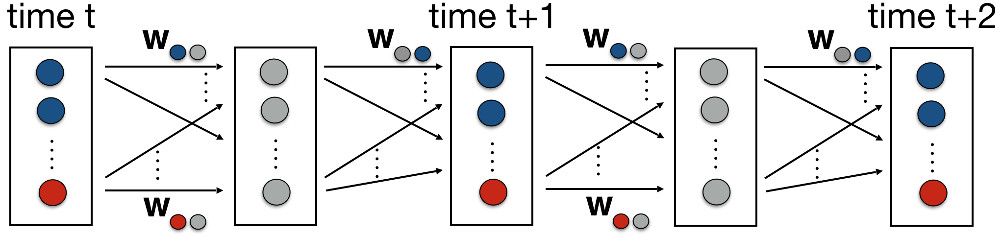
Figure 1: Visualization of the learning and planning framework [18], where blue circles represent state variables $S$, red circles represent action variables $A$, gray circles represent ReLUs $U$ and w represent the weights of a NN. During the learning stage, the weights w are learned from data. In the planning stage, the weights are fixed and the planner optimizes a given total (cumulative) reward function with respect to the set of free action variables $A$ and state variables $S$.

2.3 Mixed-Integer Linear Programming Compilation of HD-MILP-Plan

We begin with all notation necessary for HD-MILP-Plan.

2.3.1 Parameters

• $U$ is the set of ReLUs in the neural network.

• $O$ is the set of output units in the neural network.

• $w_{i,j}$ denotes the learned weight of the neural network between units $i$ and $j$.

• $A(u)$ is the set of action variables connected as inputs to unit $u\in U\cup O$.

• $S(u)$ is the set of state variables connected as inputs to unit $u\in U\cup O$.

• $U(u)$ is the set of ReLUs connected as inputs to unit $u\in U\cup O$.

• $O(s)$ specifies the output unit that predicts the value of state variable $s\in S$.

• $B(u)$ is a constant representing the bias of unit $u\in U\cup O$.

• $M$ is a large constant used in the big-M constraints.

2.3.2 Decision Variables

• ${X}_{a,t}$ is a decision variable with continuous domain denoting the value of action variable $a\in A$ at time step $t$.

• ${Y}_{s,t}$ is a decision variable with continuous domain denoting the value of state variable $s\in S$ at time step $t$.

• ${P}_{u,t}$ is a decision variable with continuous domain denoting the output of ReLU $u\in U$ at time step $t$.

• ${P}^{b}_{u,t}=1$ if ReLU $u\in U$ is activated at time step $t$, 0 otherwise (i.e., ${P}^{b}_{u,t}$ is a Boolean decision variable).

2.3.3 MILP Compilation

$$\text{maximize }\sum_{t=1}^{H}R(\langle Y_{s,t+1}|s\in S\rangle{}^{\frown}\langle X_{a,t}|a\in A\rangle)$$ (1)

subject to

$$I(\langle Y_{s,1}|s\in S\rangle)$$ (2)

$$C(\langle Y_{s,t}|s\in S\rangle{}^{\frown}\langle X_{a,t}|a\in A\rangle)$$ (3)

$$G(\langle Y_{s,H+1}|s\in S\rangle)$$ (4)

$${P}_{u,t}\leq M{P}^{b}_{u,t}\quad\forall{u\in U}$$ (5)

$${P}_{u,t}\leq M(1-{P}^{b}_{u,t})+\mathit{In}(u,t)\quad\forall{u\in U}$$ (6)

$${P}_{u,t}\geq\mathit{In}(u,t)\quad\forall{u\in U}$$ (7)

$${Y}_{s,t+1}=\mathit{In}(u,t)\quad\forall{u\in O(s),s\in S}$$ (8)

for all time steps $t=1,\dots,H$ except for constraints (2)-(4). Expression $\mathit{In}(u,t)$ denotes the total weighted input of unit $u\in U\cup O$ at time step $t$, and is equivalent to $B(u)+\sum_{u^{\prime}\in U(u)}{w_{u^{\prime},u}}{P}_{u^{\prime},t}+\sum_{s\in S(u)}{w_{s,u}}{Y}_{s,t}+\sum_{a\in A(u)}{w_{a,u}}{X}_{a,t}$.

In the above MILP, the objective function (1) maximizes the sum of rewards over a given horizon $H$. Constraints (2-4) ensure the initial state, global and goal state constraints are satisfied. Constraints (5-8) model the learned transition function $\tilde{T}$. Note that while constraints (5-7) are sufficient to encode the piecewise linear activation behaviour of ReLUs, the use of big-M constraints (5-6) can hinder the overall performance of the underlying B&B solvers that rely on the linear relaxation of the MILP. Therefore next, we turn to potential heuristics that will be used to strengthen the MILP compilation of HD-MILP-Plan.

2.4 Potential Heuristics

Potential heuristics [15, 19] are a family of heuristics that map a set of features to their numerical potentials. In the context of cost-optimal classical planning, the heuristic value of a state is defined as the sum of potentials for all the features that are true in that state. Potential heuristics provide an efficient method for computing a lower bound on the cost of a given state.

In this paper, we introduce an alternative use of potential functions to tighten the linear relaxation of ReLU units in our HD-MILP-Plan compilation and improve the search efficiency of the underlying B&B solver. We define the features of the learned NN over its set of hidden units $U$ (i.e., gray circles in Figure 1), and compute the potential contribution (i.e., reward potential) of each hidden unit $u\in U$ to the reward function $R$ for any time step $t$. These reward potentials are then used to introduce additional constraints on ReLU activations that help guide B&B search in HD-MILP-Plan. Specifically, we are interested in finding a set of reward potentials, denoted as $v^{on}_{u}$ and $v^{off}_{u}$ representing the activation (i.e., ${P}^{b}_{u,t}=1$) and the deactivation (i.e., ${P}^{b}_{u,t}=0$) of ReLUs $u\in U$, such that the relation $\sum_{u\in U}v^{on}_{u}{P}^{b}_{u,t}+v^{off}_{u}(1-{P}^{b}_{u,t})\geq R(\langle Y_{s,t+1}|s\in S\rangle{}^{\frown}\langle X_{a,t}|a\in A\rangle)$ holds for all feasible values of ${P}^{b}_{u,t}$, $Y_{s,t+1}$ and $X_{a,t}$ at any time step $t$. Once values $\bar{v}^{on}_{u}$ and $\bar{v}^{off}_{u}$ are computed, we will add $\sum_{u\in U}\bar{v}^{on}_{u}{P}^{b}_{u,t}+\bar{v}^{off}_{u}(1-{P}^{b}_{u,t})\geq R(\langle Y_{s,t+1}|s\in S\rangle{}^{\frown}\langle X_{a,t}|a\in A\rangle)$ as a linear constraint to strengthen HD-MILP-Plan. Next we describe bilevel programming that we use to model the problem of finding optimal reward potentials.

2.5 Bilevel Programming

Bilevel programming [1] is an optimization framework for modeling two-level asymetrical decision making problems with a leader and a follower problem where the leader has complete knowledge of the follower, and the follower only observes the decisions of the leader to make an optimal decision. Therefore, the leader must incorporate the optimal decision of the follower to optimize its objective.

In this work, we use bilevel programming to compactly model the problem of finding the optimal reward potentials that has exponential number of constraints. In the bilevel programming description of the optimal reward potentials problem, the leader selects the optimal values $\bar{v}^{on}_{u}$ and $\bar{v}^{off}_{u}$ of reward potentials, and the follower selects the values of ${P}^{b}_{u,t}$, $Y_{s,t+1}$ and $X_{a,t}$ such that the expression $R(\langle Y_{s,t+1}|s\in S\rangle{}^{\frown}\langle X_{a,t}|a\in A\rangle)-\sum_{u\in U}v^{on}_{u}{P}^{b}_{u,t}+v^{off}_{u}(1-{P}^{b}_{u,t})$ is maximized. That is, the follower tries to find values of ${P}^{b}_{u,t}$, $Y_{s,t+1}$ and $X_{a,t}$ that violate the relation $\sum_{u\in U}v^{on}_{u}{P}^{b}_{u,t}+v^{off}_{u}(1-{P}^{b}_{u,t})\geq R(\langle Y_{s,t+1}|s\in S\rangle{}^{\frown}\langle X_{a,t}|a\in A\rangle)$ as much as possible. Therefore the leader must select the values $\bar{v}^{on}_{u}$ and $\bar{v}^{off}_{u}$ of reward potentials by incorporating the optimal decision making model of the follower. Next, we describe the reward potentials for learned NNs.

3 Reward Potentials for Learned Neural Networks

In this section, we present the optimal reward potentials problem and an efficient constraint generation framework for finding reward potentials for learned NNs.

3.1 Optimal Reward Potentials Problem

The problem of finding the optimal reward potentials over a set of ReLUs $U$ for any time step $t$ can be defined as the following bilevel optimization problem.

3.1.1 Leader Problem

$$\min_{v^{on}_{u},v^{off}_{u},Y_{s,t},Y_{s,t+1},X_{a,t},{P}^{b}_{u,t}}\sum_{u\in U}v^{on}_{u}+v^{off}_{u}$$ (9)

subject to

$$\sum_{u\in U}v^{on}_{u}{P}^{b}_{u,t}+v^{off}_{u}(1-{P}^{b}_{u,t})\geq R(\langle Y_{s,t+1}|s\in S\rangle{}^{\frown}\langle X_{a,t}|a\in A\rangle)$$ (10)

$$Y_{s,t},Y_{s,t+1},X_{a,t},{P}^{b}_{u,t}\in\arg\text{Follower Problem}$$

3.1.2 Follower Problem

$$\max_{Y_{s,t},Y_{s,t+1},X_{a,t},{P}^{b}_{u,t}}R(\langle Y_{s,t+1}|s\in S\rangle{}^{\frown}\langle X_{a,t}|a\in A\rangle)-\sum_{u\in U}v^{on}_{u}{P}^{b}_{u,t}+v^{off}_{u}(1-{P}^{b}_{u,t})$$ (11)

subject to

Constraints (3) and (5-8)

In the above bilevel problem, the leader problem selects the values $\bar{v}^{on}_{u}$ and $\bar{v}^{off}_{u}$ of the reward potentials such that their total sum is minimized (i.e., objective function (9)), and their total weighted sum for all ReLU activations is an upper bound to all values of the reward function $R$ (i.e., constraint (10) and the follower problem). Given the values $\bar{v}^{on}_{u}$ and $\bar{v}^{off}_{u}$ of the reward potentials, the follower selects the values of decision variables $Y_{s,t}$, $Y_{s,t+1}$, $X_{a,t}$ and ${P}^{b}_{u,t}$ such that the difference between the value of the reward function $R$ and the sum of reward potentials is maximized subject to constraints (3) and (5-8). Next, we show the correctness of the optimal reward potentials problem as the bilevel program described by the leader (i.e., objective function (9) and constraint (10)) and the follower (i.e., objective function (11) and constraints (3) and (5-8)) problems.

Theorem 3.1 (Correctness of The Optimal Reward Potentials Problem)

Given constraints (3) and (5-8) are feasible, the optimal reward potentials problem finds the values $\bar{v}^{on}_{u}$ and $\bar{v}^{off}_{u}$ of reward potentials such that the relation $\sum_{u\in U}\bar{v}^{on}_{u}{P}^{b}_{u,t}+\bar{v}^{off}_{u}(1-{P}^{b}_{u,t})\geq R(\langle Y_{s,t+1}|s\in S\rangle{}^{\frown}\langle X_{a,t}|a\in A\rangle)$ holds for all values of ${P}^{b}_{u,t}$, $Y_{s,t+1}$ and $X_{a,t}$ at any time step $t$.

Proof (by Contradiction)

Let $\bar{v}^{on}_{u}$ and $\bar{v}^{off}_{u}$ denote the values of reward potentials selected by the leader problem that violate the relation $\sum_{u\in U}\bar{v}^{on}_{u}{P}^{b}_{u,t}+\bar{v}^{off}_{u}(1-{P}^{b}_{u,t})\geq R(\langle Y_{s,t+1}|s\in S\rangle{}^{\frown}\langle X_{a,t}|a\in A\rangle)$ for some values $\bar{Y}_{s,t+1}$, $\bar{X}_{a,t}$ and $\bar{P}^{b}_{u,t}$, implying $R(\langle\bar{Y}_{s,t+1}|s\in S\rangle{}^{\frown}\langle\bar{X}_{a,t}|a\in A\rangle)-\sum_{u\in U}\bar{v}^{on}_{u}\bar{P}^{b}_{u,t}+\bar{v}^{off}_{u}(1-\bar{P}^{b}_{u,t})>0$. However, the feasibility of constraint (10) implies that the value of the objective function (11) must be non-positive (i.e., the follower problem is not solved to optimality), which yields the desired contradiction.

Note that we omit the case when constraints (3) and (5-8) are infeasible because it implies the infeasibility of the learned planning problem $\tilde{\Pi}$. Next, we describe a finite-time constraint generation algorithm for computing reward potentials.

3.2 Constraint Generation for Computing Reward Potentials

The optimal reward potentials problem can be solved efficiently through the following constraint generation framework that decomposes the problem into a master problem and a subproblem. The master problem finds the values $\bar{v}^{on}_{u}$ and $\bar{v}^{off}_{u}$ of ReLU potential variables. The subproblem finds the values $\bar{P}^{b}_{u,t}$ of ReLU variables that violate constraint (10) the most for given values $\bar{v}^{on}_{u}$ and $\bar{v}^{off}_{u}$, and also finds the maximum value of reward function $R$ for given $\bar{P}^{b}_{u,t}$ which is denoted as $R^{*}(\langle\bar{P}^{b}_{u,t}|u\in U\rangle)$. Intuitively, the master problem selects the values $\bar{v}^{on}_{u}$ and $\bar{v}^{off}_{u}$ of ReLU potentials that are checked by the subproblem for the validity of the relation $\sum_{u\in U}\bar{v}^{on}_{u}{P}^{b}_{u,t}+\bar{v}^{off}_{u}(1-{P}^{b}_{u,t})\geq R(\langle Y_{s,t+1}|s\in S\rangle{}^{\frown}\langle X_{a,t}|a\in A\rangle)$ for all feasible values of ${P}^{b}_{u,t}$, $Y_{s,t+1}$ and $X_{a,t}$ at any time step $t$. If a violation is found, a linear constraint corresponding to a given $\bar{P}^{b}_{u,t}$ and $R^{*}(\langle\bar{P}^{b}_{u,t}|u\in U\rangle)$ is added back to the master problem and the procedure is repeated until no violation is found by the subproblem.

3.2.1 Subproblem $\mathcal{S}$:

For a complete value assignment $\bar{v}^{on}_{u}$ and $\bar{v}^{off}_{u}$ to ReLU potential variables, the subproblem optimizes the violation (i.e., objective function (11)) with respect to constraints (3) and (5-8) as follows.

$$\max_{Y_{s,t},Y_{s,t+1},X_{a,t},{P}^{b}_{u,t}}R(\langle Y_{s,t+1}|s\in S\rangle{}^{\frown}\langle X_{a,t}|a\in A\rangle)-\sum_{u\in U}\bar{v}^{on}_{u}{P}^{b}_{u,t}+\bar{v}^{off}_{u}(1-{P}^{b}_{u,t})$$ (12)

subject to

Constraints (3) and (5-8)

We denote the optimal values of ReLU variables ${P}^{b}_{u,t}$, found by solving the subproblem as $\bar{P}^{b}_{u,t}$, and the value of the reward function $R$ found by solving the subproblem as $R^{*}(\langle\bar{P}^{b}_{u,t}|u\in U\rangle)$. Further, we refer to subproblem as $\mathcal{S}$.

3.2.2 Master problem $\mathcal{M}$:

Given the set of complete value assignments $K$ to ReLU variables with values $\bar{P}^{b,k}_{u,t}$ and optimal objective values $R^{*}(\langle\bar{P}^{b,k}_{u,t}|u\in U\rangle)$ for all $k\in K$, the master problem optimizes the regularized sum of reward potentials (i.e., regularized objective function (9)) with respect to the modified version of constraint (10) as follows.

$$\min_{v^{on}_{u},v^{off}_{u}}\sum_{u\in U}v^{on}_{u}+v^{off}_{u}+\lambda\sum_{u\in U}(v^{on}_{u})^{2}+(v^{off}_{u})^{2}$$ (13)

subject to

$$\sum_{u\in U}v^{on}_{u}\bar{P}^{b,k}_{u,t}+v^{off}_{u}(1-\bar{P}^{b,k}_{u,t})\geq R^{*}(\langle\bar{P}^{b,k}_{u,t}|u\in U\rangle)\quad\forall{k\in K}$$ (14)

We denote the optimal values of ReLU potential variables $v^{on}_{u}$ and $v^{off}_{u}$, found by solving the master problem as $\bar{v}^{on}_{u}$ and $\bar{v}^{off}_{u}$, respectively. Further, we refer to master problem as $\mathcal{M}$.

3.2.3 Reward Potentials Algorithm

Given the definitions of the master problem $\mathcal{M}$ and the subproblem $\mathcal{S}$, the constraint generation algorithm for computing an optimal reward potential is outlined as follows.

Algorithm 1 Reward Potentials Algorithm

1:$\textit{k}\leftarrow 1$, violation $\leftarrow\infty$, $\mathcal{M}\leftarrow$ objective function (13)

2:while violation $>$ 0 do

3:    $\bar{v}^{on}_{u},\bar{v}^{off}_{u}\leftarrow\mathcal{M}$

4:    $\bar{P}^{b,k}_{u,t},\bar{Y}_{s,t+1},\bar{X}_{a,t},R^{*}(\langle\bar{P}^{b,k}_{u,t}|u\in U\rangle)\leftarrow\mathcal{S}(\bar{v}^{on}_{u},\bar{v}^{off}_{u})$

5:    violation = $R(\langle\bar{Y}_{s,t+1}|s\in S\rangle{}^{\frown}\langle\bar{X}_{a,t}|a\in A\rangle)-\sum_{u\in U}\bar{v}^{on}_{u}\bar{P}^{b,k}_{u,t}+\bar{v}^{off}_{u}(1-\bar{P}^{b,k}_{u,t})$

6:    $\mathcal{M}\leftarrow\mathcal{M}\cup\sum_{u\in U}v^{on}_{u}\bar{P}^{b,k}_{u,t}+v^{off}_{u}(1-\bar{P}^{b,k}_{u,t})\geq R^{*}(\langle\bar{P}^{b,k}_{u,t}|u\in U\rangle)$ (i.e., update constraint (14))

7:    $k\leftarrow k+1$

Given constraints (3) and (5-8) are feasible, Algorithm 1 iteratively computes reward potentials $v^{on}_{u}$ and $v^{off}_{u}$ (i.e., line 3), and first checks if there exists an activation pattern, that is a complete value assignment $\bar{P}^{b,k}_{u,t}$ to ReLU variables, that violates constraint (10) (i.e., lines 4 and 5), and then returns the optimal reward value $R^{*}(\langle\bar{P}^{b,k}_{u,t}|u\in U\rangle)$ for the violating activation pattern. Given the optimal reward value $R^{*}(\langle\bar{P}^{b,k}_{u,t}|u\in U\rangle)$ for the violating activation pattern, constraint (14) is updated (i.e., lines 6-7). Since there are finite number of activation patterns and solving $\mathcal{S}$ gives the maximum value of $R^{*}(\langle\bar{P}^{b,k}_{u,t}|u\in U\rangle)$ for each pattern $k\in\{1,\dots,2^{|U|}\}$, the Reward Potentials Algorithm 1 terminates in at most $k\leq 2^{|U|}$ iterations with an optimal reward potential for the learned NN.

3.2.4 Increasing the Granularity of the Reward Potentials Algorithm

The feature space of Algorithm 1 can be enhanced to include information on each ReLUs input and/or output. Instead of computing reward potentials for only the activation $\bar{v}^{on}_{u}$ and deactivation $\bar{v}^{off}_{u}$ of ReLU $u\in U$, we (i) introduce an interval parameter $N$ to split the output range of each ReLU $u$ into $N$ equal size intervals, (ii) introduce auxiliary Boolean decision variables ${P^{\prime}}^{b}_{i,u,t}$ to represent the activation interval of ReLU $u$ such that ${P^{\prime}}^{b}_{i,u,t}=1$ if and only if the output of ReLU $u$ is within interval $i\in\{1,\dots,N\}$, and ${P^{\prime}}^{b}_{i,u,t}=0$ otherwise, and (iii) compute reward potentials for each activation interval $\bar{v}^{on}_{u,1},\dots,\bar{v}^{on}_{u,N}$ and deactivation $\bar{v}^{off}_{u}$ of ReLU $u\in U$.

3.3 Strengthening HD-MILP-Plan

Given optimal reward potentials $\bar{v}^{on}_{u,1},\dots,\bar{v}^{on}_{u,N}$ and $\bar{v}^{off}_{u}$, the MILP compilation of HD-MILP-Plan is strengthened through the addition of following constraints:

$$\sum_{u\in U}\sum^{N}_{i=1}\bar{v}^{on}_{u,i}{P^{\prime}}^{b}_{i,u,t}+\bar{v}^{off}_{u}(1-x^{t}_{u})\geq R(\langle Y_{s,t+1}|s\in S\rangle{}^{\frown}\langle X_{a,t}|a\in A\rangle)$$ (15)

$$\sum^{N}_{i=1}{P^{\prime}}^{b}_{i,u,t}={P}^{b}_{u,t}$$ (16)

$$N_{u}\frac{(i-1)}{N}{P^{\prime}}^{b}_{i,u,t}\leq{P}_{u,t}\leq N_{u}-(N_{u}-N_{u}\frac{i}{N}){P^{\prime}}^{b}_{i,u,t}\quad\forall{i\in\{1,\dots,N\},u\in U}$$ (17)

for all time steps $t\in\{1,\dots,H\}$ where $N_{u}$ denotes the upperbound obtained from performing forward reachability on the output of each ReLU $u\in U$ in the learned NN. Briefly, constraint (15) provides the upperbound on the reward function $R$ as a function of ReLU activation intervals and deactivations. Constraint (16) ensures that (i) at most one auxillary variable ${P^{\prime}}^{b}_{i,u,t}$ is selected, and (ii) at least one auxillary variable ${P^{\prime}}^{b}_{i,u,t}$ is selected if and only if ReLU $u$ is activated. Constraint (17) ensures that the output of each ReLU is within its selected activation interval. Next, we present our experimental results to demonstrate the efficiency and the utility of computing reward potential and strengthening HD-MILP-Plan.

4 Experimental Results

In this section, we present computational results on (i) the convergence of Algorithm 1, and (ii) the overall strengthening of HD-MILP-Plan with the addition of constraints (15-17) for the task of planning over long horizons. First, we present results on the overall efficiency of Algorithm 1 and the strengthening of HD-MILP-Plan over multiple learned planning instances. Then, we focus on the most computationally expensive domain identified by our experiments to further investigate the convergence behaviour of Algorithm 1 and the overall strengthening of HD-MILP-Plan as a function of time.

4.1 Experimental Setup

The experiments were run on a MacBookPro with 2.8 GHz Intel Core i7 16GB memory. All instances and the respective learned neural networks from the HD-MILP-Plan paper [18], namely Navigation, Reservoir Control and HVAC [18], were selected. Both domain instance sizes and their respective learned NN sizes are detailed in Table 1 where columns from left to right denote the name of problem instances, the structures of the learned NNs where each number denotes the width of a layer and the values of the planning horizon $H$, respectively. The range bounds on action variables for Navigation domains were constrained to $[-0.1,0.1]$. CPLEX 12.9.0 [8] solver was used to optimize both Algorithm 1, and HD-MILP-PLan, with 6000 seconds of total time limit per domain instance. In our experiments, we show results for the base model (i.e., objective (1) and constraints (2-8)) and the strengthened model with the addition of constraints (15-17) for the values of interval parameter $N=2,3$. Finally in the master problem, we have chosen the regularizer constant $\lambda$ in the objective function (9) to be $\frac{1}{\sqrt{M}}$ where $M$ is the large constant used in the big-M constraints of HD-MILP-Plan (i.e., constraints (5-6)).

Table 1: Domain and learned NN descriptions where columns from left to right denote the name of problem instances, the structures of NNs used to learn each transition model $\tilde{T}$ where each number denotes the width of a layer, and the values of the planning horizon $H$, respectively.

Domain Instance	Network Structure	Horizon
Navigation (8-by-8 maze)	4:32:32:2	100
Navigation (10-by-10 maze)	4:32:32:2	100
Reservoir Control (3 reservoirs)	6:32:3	500
Reservoir Control (4 reservoirs)	8:32:4	500
HVAC (3 rooms)	6:32:3	100
HVAC (6 rooms)	12:32:6	100

4.2 Overall Results

In this section, we present the experimental results on (i) the computation of the optimal reward potentials using Algorithm 1, (ii) and the performance of HD-MILP-Plan with the addition of constraints (15-17) over multiple learned planning instances over long horizons. Table 2 summarizes the computational results and highlights the best performing HD-MILP-Plan settings for each learned planning instance.

Table 2: Summary of experimental results on the computationally efficiency of Algorithm 1 and HD-MILP-Plan with the addition of constraint (15-17) over multiple learned planning instances with long horizons.

Domain Setting	Alg. 1	Cumul.	Primal	Dual	Open	Closed
Nav,8,100,Base	-	6000	-	-261.4408	16536	27622
Nav,8,100,N=2	345	6000	-	-267.1878	6268	15214
Nav,8,100,N=3	1150	6000	-	-267.056	6189	12225
Nav,10,100,Base	-	6000	-	-340.5974	17968	35176
Nav,10,100,N=2	800	6000	-	-340.6856	14435	27651
Nav,10,100,N=3	1700	6000	-	-339.8124	2593	7406
HVAC,3,100,Base	-	260.21	Opt. found	Opt. proved	0	289529
HVAC,3,100,N=2	7	88.21	Opt. found	Opt. proved	0	2501
HVAC,3,100,N=3	9	194.44	Opt. found	Opt. proved	0	10891
HVAC,6,100,Base	-	6000	-1214369.086	-1213152.304	618687	648207
HVAC,6,100,N=2	8	6000	-1214365.427	-1213199.787	554158	567412
HVAC,6,100,N=3	10	6000	-1214364.704	-1213025.189	1011348	1021637
Res,3,500,Base	-	33.01	Opt. found	Opt. proved	0	1
Res,3,500,N=2	1	99.81	Opt. found	Opt. proved	0	714
Res,3,500,N=3	2	90.27	Opt. found	Opt. proved	0	674
Res,4,500,Base	-	300.71	Opt. found	Opt. proved	0	1236
Res,4,500,N=2	7	109.66	Opt. found	Opt. proved	0	1924
Res,4,500,N=3	6	232.19	Opt. found	Opt. proved	0	1294

The first column of Table 2 identifies the domain setting of each row. The second column denotes the runtime of Algorithm 1 in seconds. The third column (i.e., Cumul.) denotes the cumulative runtime of Algorithm 1 and HD-MILP-Plan in seconds. The remaining columns provide information on the performance of HD-MILP-Plan. Specifically, the fourth column (i.e., Primal) denotes the value of the incumbent plan found by HD-MILP-Plan, the fifth column (i.e., Dual) denotes the value of the duality bound found by HD-MILP-Plan, and the sixth and seventh columns (i.e., Open and Closed) denote the number of open and closed nodes in the B&B tree respectively. The bolded values indicate the best performing HD-MILP-Plan settings for each learned planning instance where the performance of each setting is evaluated first based on the runtime performance (i.e., Cumul. column), followed by the quality of incumbent plan (i.e., Primal column) and duality bound (i.e., Dual column) obtained by HD-MILP-Plan.

In total of five out of six instances, we observe that strengthened HD-MILP-Plan with interval parameter $N=2$ performed the best. The pairwise comparison of the base HD-MILP-Plan and strengthened HD-MILP-Plan with interval parameter $N=3$ shows that in almost all instances, the strengthened model performed better in comparison to the base model. The only instance in which the base model significantly outperformed the other two was the Reservoir Control domain with three reservoirs where the B&B solver was able to find an optimal plan in the root node. Overall, we found that especially in the instances where the optimality was hard to prove within the runtime limit of 6000 seconds (i.e., all Navigation instances and HVAC domain with 6 rooms), strengthened HD-MILP-Plan explored signigicantly less number of nodes in general while obtaining either higher quality incumbent plans or lower dual bounds. We observe that Algorithm 1 terminated with optimal reward potentials in less than 10 seconds in both Reservoir Control and HVAC domains, and took as much as 1700 seconds in Navigation domain – highlighting the effect of NN size and complexity (i.e., detailed in Table 1) on the runtime of Algorithm 1. As a result, next we focus on the most computationally expensive domain identified by our experiments, namely Navigation, to get a better understanding on the convergence behaviour of Algorithm 1 and the overall efficiency of HD-MILP-Plan as a function of time.

4.3 Detailed Convergence Results on Navigation Domain

In this section, we inspect the convergence of Algorithm 1 in the Navigation domain for computing an optimal reward potential for the learned NNs.

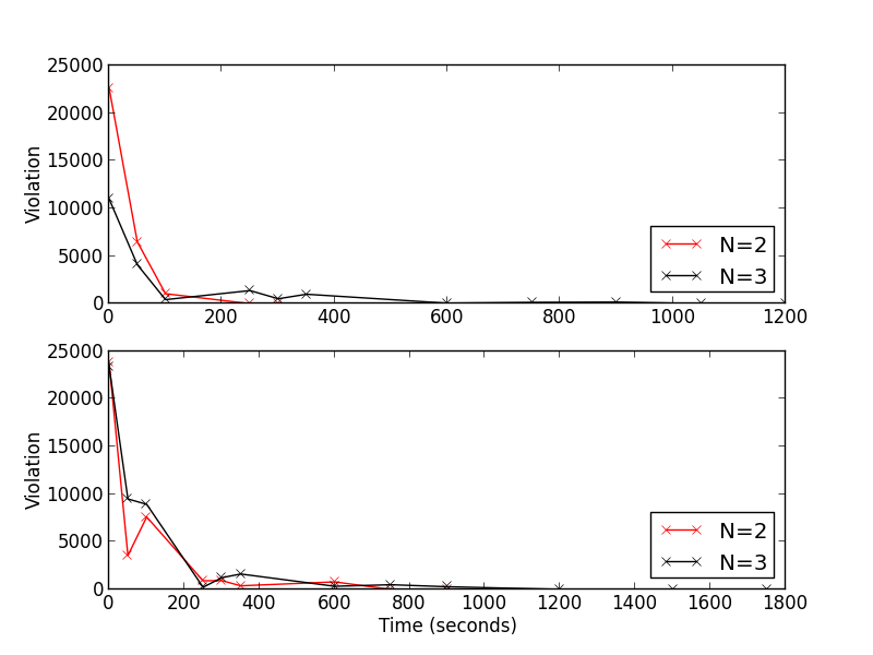
Figure 2: Convergence of Algorithm 1 as a function of time for the learned NNs of both Navigation 8-by-8 (i.e., top) and Navigation 10-by-10 (i.e., bottom) planning instances. The violation of constraint (10) decreases exponentially as a function of time, showcasing a long-tail runtime behaviour and terminates with optimal reward potentials.

Figure 2 visualizes the violation of constraint (10) as a function of time over the computation of optimal reward potentials using the Reward Potentials Algorithm 1 for the learned NNs of both Navigation 8-by-8 (i.e., top) and Navigation 10-by-10 (i.e., bottom) planning instances. In both, we observe that the violation of constraint (10) decreases exponentially as a function of time, showcasing a long-tail runtime behaviour and terminates with optimal reward potentials.

4.4 Detailed Strengthening Results on Navigation Domain

Next, we inspect the overall strengthening of HD-MILP-Plan with respect to its underlying linear relaxation and search efficiency as a result of constraints (15-17), for the task of planning over long horizons in the Navigation domain.

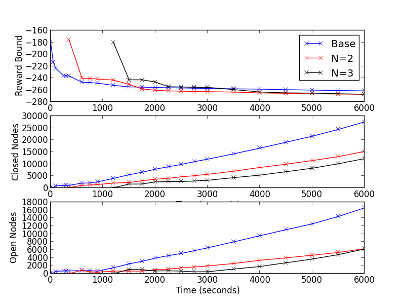
Figure 3: Linear relaxation and search efficiency comparisons in Navigation domain with an 8-by-8 maze between the base and the strengthened HD-MILP-Plan using Algorithm 1 with interval parameter $N=2,3$. Overall, we observe that HD-MILP-Plan with constraints (15-17) outperforms the base HD-MILP-Plan by 1700 and 3300 seconds with interval parameter $N=2,3$, respectively.

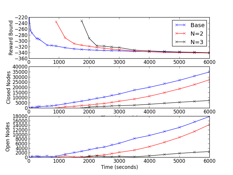
Figure 4: Linear relaxation and search efficiency comparisons in Navigation domain with an 10-by-10 maze between the base and the strengthened HD-MILP-Plan using Algorithm 1 with interval parameter $N=2,3$. Overall, we observe that HD-MILP-Plan with constraints (15-17) obtains a tighter bound compared to the base HD-MILP-Plan by 3750 seconds and reaches almost the same bound by the time limit (i.e., 6000 seconds) with interval parameter $N=2,3$, respectively.

Figures 3 and 4 visualize the overall effect of incorporating constraints (15-17) into HD-MILP-Plan as a function of time for the Navigation domain with (a) 8-by-8 and (b) 10-by-10 maze sizes. In both Figures 3 and 4, linear relaxation (i.e. top), number of closed nodes (i.e., middle), and number open nodes (i.e., bottom), are displayed as a function of time. The inspection of both Figures 3 and 4 show that once the reward potentials are computed, the addition of constraints (15-17) allows HD-MILP-Plan to obtain a tighter bound by exploring signigicantly less number of nodes. In the 8-by-8 maze instance, we observe that HD-MILP-Plan with constraints (15-17) outperforms the base HD-MILP-Plan by 1700 and 3300 seconds with interval parameter $N=2,3$, respectively. In the 10-by-10 maze instance, we observe that HD-MILP-Plan with constraints (15-17) obtains a tighter bound compared to the base HD-MILP-Plan by 3750 seconds and almost reaches the same bound by the time limit (i.e., 6000 seconds) with interval parameter $N=2,3$, respectively.

The inspection of the top subfigures in Figures 3 and 4 shows that increasing the value of the interval parameter $N$ increases the computation time of Algorithm 1, but can also increase the search efficiency of the underlying B&B solver through increasing its exploration and pruning capabilities, as demonstrated by the middle and bottom subfigures in Figures 3 and 4. Overall from both instances, we conclude that HD-MILP-Plan with constraints (15-17) obtains a linear relaxation that is at least as good as the base HD-MILP-Plan by exploring significantly less number of nodes in the B&B search tree.

5 Related Work

In this paper, we have focused on the important problem of improving the efficiency of B&B solvers for optimal planning with learned NN transition models in continuous action and state spaces. Parallel to this work, planning and decision making in discrete action and state spaces [12, 17, 16], verification of learned NNs [9, 6, 7, 14], robustness evaluation of learned NNs [20] and defenses to adversarial attacks for learned NNs [10] have been studied with the focus of solving very similar decision making problems. For example, the verification problem solved by Reluplex [9] is very similar to the planning problem solved by HD-MILP-Plan [18] without the objective function and horizon $H=1$. Interestingly, the verification problem can also be modeled as an optimization problem [2] and potentially benefit from the findings presented in this paper. For future work, we plan to explore how our findings in this work translate to solving other important tasks for learned neural networks.

6 Conclusion

In this paper, we have focused on the problem of improving the linear relaxation and the search efficiency of MILP models for decision making with learned NNs. In order to tacke this problem, we used bilevel programming to correctly model the optimal reward potentials problem. We then introduced a novel finite-time constraint generation algorithm for computing the potential contribution of each hidden unit to the reward function of the planning problem. Given the precomputed values of the reward potentials, we have introduced constraints to tighten the bound on the reward function of the planning problem. Experimentally, we have shown that our constraint generation algorithm efficiently computes reward potentials for learned NNs, and the overhead computation is justified by the overall strengthening of the underlying MILP model as demonstrated on the task of planning over long horizons. With this paper, we have shown the potential of bridging the gap between two seemingly distant literatures; the research on planning heuristics and decision making with learned NN models in continuous action and state spaces.

References

- [1] Bard, J.: Practical Bilevel Optimization: Algorithms And Applications. Springer US (09 2000). https://doi.org/10.1007/978-1-4757-2836-1
- [2] Bunel, R., Turkaslan, I., Torr, P.H., Kohli, P., Kumar, M.P.: A unified view of piecewise linear neural network verification (2017)
- [3] Clarke, E., Grumberg, O., Jha, S., Lu, Y., Veith, H.: Counterexample-guided abstraction refinement. In: Emerson, E.A., Sistla, A.P. (eds.) Computer Aided Verification. pp. 154–169. Springer Berlin Heidelberg, Berlin, Heidelberg (2000)
- [4] Collobert, R., Weston, J., Bottou, L., Karlen, M., Kavukcuoglu, K., Kuksa, P.: Natural language processing (almost) from scratch. Journal of Machine Learning Research 12, 2493–2537 (2011)
- [5] Deng, L., Hinton, G.E., Kingsbury, B.: New types of deep neural network learning for speech recognition and related applications: an overview. In: IEEE International Conference on Acoustics, Speech and Signal Processing. pp. 8599–8603 (2013)
- [6] Ehlers, R.: Formal verification of piece-wise linear feed-forward neural networks. In: D’Souza, D., Narayan Kumar, K. (eds.) Automated Technology for Verification and Analysis. pp. 269–286. Springer International Publishing, Cham (2017)
- [7] Huang, X., Kwiatkowska, M., Wang, S., Wu, M.: Safety verification of deep neural networks. In: Majumdar, R., Kunčak, V. (eds.) Computer Aided Verification. pp. 3–29. Springer International Publishing, Cham (2017)
- [8] IBM: IBM ILOG CPLEX Optimization Studio CPLEX User’s Manual (2019)
- [9] Katz, G., Barrett, C., Dill, D., Julian, K., Kochenderfer, M.: Reluplex: An efficient smt solver for verifying deep neural networks. In: Twenty-Ninth International Conference on Computer Aided Verification. CAV (2017)
- [10] Kolter, Zico, W., Eric: Provable defenses against adversarial examples via the convex outer adversarial polytope. In: Thirty-First Conference on Neural Information Processing Systems (2017)
- [11] Krizhevsky, A., Sutskever, I., Hinton, G.E.: Imagenet classification with deep convolutional neural networks. In: Twenty-Fifth Neural Information Processing Systems. pp. 1097–1105 (2012), http://dl.acm.org/citation.cfm?id=2999134.2999257
- [12] Lombardi, M., Gualandi, S.: A lagrangian propagator for artificial neural networks in constraint programming. vol. 21, pp. 435–462 (Oct 2016). https://doi.org/10.1007/s10601-015-9234-6, https://doi.org/10.1007/s10601-015-9234-6
- [13] Nair, V., Hinton, G.E.: Rectified linear units improve restricted boltzmann machines. In: Twenty-Seventh International Conference on Machine Learning. pp. 807–814 (2010), http://www.icml2010.org/papers/432.pdf
- [14] Narodytska, N., Kasiviswanathan, S., Ryzhyk, L., Sagiv, M., Walsh, T.: Verifying properties of binarized deep neural networks. In: Thirty-Second AAAI Conference on Artificial Intelligence. pp. 6615–6624 (2018)
- [15] Pommerening, F., Helmert, M., R¨oger, G., Seipp, J.: From non-negative to general operator cost partitioning. In: Twenty-Ninth AAAI Conference on Artificial Intelligence. pp. 3335–3341 (2015)
- [16] Say, B., Sanner, S.: Compact and efficient encodings for planning in factored state and action spaces with learned binarized neural network transition models (2018)
- [17] Say, B., Sanner, S.: Planning in factored state and action spaces with learned binarized neural network transition models. In: Twenty-Seventh International Joint Conference on Artificial Intelligence. pp. 4815–4821 (2018). https://doi.org/10.24963/ijcai.2018/669, https://doi.org/10.24963/ijcai.2018/669
- [18] Say, B., Wu, G., Zhou, Y.Q., Sanner, S.: Nonlinear hybrid planning with deep net learned transition models and mixed-integer linear programming. In: Twenty-Sixth International Joint Conference on Artificial Intelligence. pp. 750–756 (2017). https://doi.org/10.24963/ijcai.2017/104, https://doi.org/10.24963/ijcai.2017/104
- [19] Seipp, J., Pommerening, F., Helmert, M., R¨oger: New optimization functions for potential heuristics. In: Twenty-Fifth International Conference on Automated Planning and Scheduling. pp. 193–201 (2015)
- [20] Tjeng, V., Xiao, K., Tedrake, R.: Evaluating robustness of neural networks with mixed integer programming. In: Seventh International Conference on Learning Representations (2019)