Multi-jet merging in a variable flavor number scheme

Abstract

We propose a novel technique for the combination of multi-jet merged simulations in the five-flavor scheme with calculations for the production of $b$-quark associated final states in the four-flavor scheme. We show the equivalence of our algorithm to the FONLL method at the fixed-order and logarithmic accuracy inherent to the matrix-element and parton-shower simulation employed in the multi-jet merging. As a first application we discuss $Zb\bar{b}$ production at the Large Hadron Collider.

I Introduction

Measurements involving heavy-flavor (HF) production are a vital component of the physics program at the Large Hadron Collider (LHC). With the Higgs boson decaying predominantly into $b$ quarks, some of the recent efforts in the LHC experiments have focused on this decay mode in Higgs production in association with vector bosons Aaboud et al. (2018a); Sirunyan et al. (2018a) and in association with top quarks Sirunyan et al. (2018b); Aaboud et al. (2018b). Furthermore, searches for physics beyond the Standard Model (SM) also often rely on heavy flavor final states because the couplings to third generation fermions are sometimes assumed to be enhanced in new physics models. While the modeling of signal processes is relevant, it is of even higher importance to have a precise prediction for the dominant SM backgrounds including heavy flavor production. This is reflected for example by the large efforts spent in the LHC Higgs Cross Section Working Group de Florian et al. (2016) to understand the modeling of the $t\bar{t}b\bar{b}$ background to $t\bar{t}H(b\bar{b})$.

Including heavy-quark mass effects in the QCD evolution, e.g. in fits of parton distribution functions (PDFs), is a prerequisite. The fixed flavor number scheme (FFNS) as the simplest approach assumes a fixed number of active quarks which can be varied explicitly Alekhin et al. (2010). General-mass variable flavor number schemes (VFNS) like ACOT Aivazis et al. (1994a, b); Tung et al. (2002); Kniehl et al. (2011), TR Thorne and Roberts (1998); Thorne (2006), and FONLL Cacciari et al. (1998); Forte et al. (2010) on the other hand account for mass effects dynamically above the corresponding thresholds. Hybrid schemes have also been devised Kusina et al. (2013), and the possibility to perform the PDF evolution for massive quarks has been investigated recently Krauss and Napoletano (2018). Accordingly, higher-order corrections to the production of a final state like $Hb\bar{b}$ or $Zb\bar{b}$ have been computed for a fixed number of flavors Dittmaier et al. (2004); Dawson et al. (2004); Febres Cordero et al. (2008, 2009); Campbell et al. (2012), and in variable flavor number schemes Campbell et al. (2009); Forte et al. (2015, 2016, 2018); Bonvini et al. (2015, 2016). Progress in clarifying the interplay between different schemes was reviewed in Febres Cordero and Reina (2015), and the effect of higher-order electroweak corrections was investigated recently Figueroa et al. (2018).

For experimental analyses a realistic simulation of collision events at the hadron level is crucial. Such simulations are provided by all modern Monte Carlo event generators Buckley et al. (2011) like Herwig7 Bellm et al. (2016), Pythia8 Sjöstrand et al. (2014) and Sherpa Gleisberg et al. (2009). The simulation of heavy-flavor production employed in these programs varies both in method and in accuracy, and a formal comparison to the methods used in analytical calculations is missing so far. Typical event generator setups employ matrix elements in the five-flavor scheme (5FS), where the $b$-quark is treated as massless and included also as an initial state parton. Before the parton shower is simulated, $b$-quark masses are restored by means of a kinematics reshuffling, and subsequently massive splitting kernels and kinematics are used in the parton shower, see e.g. Norrbin and Sjöstrand (2001); Schumann and Krauss (2008); Höche and Prestel (2015); Cabouat and Sjöstrand (2018); Cormier et al. (2018). This procedure is necessary in particular to avoid an excess in the $g\to bb$ splitting rate as it would appear if the fragmentation process was simulated with massless $b$-quarks.

To increase the accuracy of heavy-flavor production Monte Carlo samples, two approaches have been studied in the literature: The matching of NLO QCD calculations in the four-flavor scheme (4FS) to parton showers using one of the common NLO+PS matching formalisms Frixione and Webber (2002); Nason (2004); Frixione et al. (2007); Höche et al. (2012); Plätzer and Gieseke (2012). This method has been used to simulate for example the $pp\to Vbb$ process class Frederix et al. (2011); Oleari and Reina (2011); Bagnaschi et al. (2018); Krauss et al. (2017) and the $pp\to ttbb$ process Cascioli et al. (2013); Ježo et al. (2018); Bevilacqua et al. (2017). An alternative option to include higher-order QCD corrections in MCs is the use of multi-leg merging methods at LO Catani et al. (2001); Mangano et al. (2002); Krauss (2002); Lönnblad (2002); Lavesson and Lönnblad (2008); Alwall et al. (2008); Höche et al. (2009); Hamilton et al. (2009); Lönnblad and Prestel (2012) or NLO Höche et al. (2013); Gehrmann et al. (2013); Lönnblad and Prestel (2013); Frederix and Frixione (2012); Bellm et al. (2018) accuracy. Heavy-flavor production is then included automatically in the 5FS using massless matrix elements and a massive parton shower as described above. Dedicated studies of this and a comparison to the 4FS can be found in Krauss et al. (2017).

In this paper we propose a novel method that presents a hybrid between these two approaches. Embedding a massive NLO+PS calculation for $pp\to Zbb$ into a massless multi-leg merging of $pp\to Z$+jets we retain the theoretical advantages of both methods and for the first time allow a rigorous combination of the two calculations without overlap. The latter is not merely a technical or academic point, but crucial to allow the usage of NLO-accurate heavy flavor predictions in experiments: If heavy flavor and light jet production can not be described simultaneously, it is impossible to make predictions in the presence of fake heavy flavor jets or evaluate experimental efficiencies related to them.

This paper is organized as follows: After a short review of multi-jet merging in Sec. II, we describe our method from an algorithmic point of view in Sec. III. Its formal relation to the FONLL method is studied in Sec. IV. Finally, in Sec. V we demonstrate an implementation of the new method within the Sherpa event generator using $pp\to Zb\bar{b}$ production as a test case.

II Multi-jet merging in a fixed flavor number scheme

In the context of Monte-Carlo event generators, multi-jet merging refers to algorithms that systematically improve the accuracy of traditional LO+PS simulations by adding higher multiplicity fixed-order calculations with well-separated parton-level jets to the simulation. Merging algorithms are constructed such as to obtain a consistent result that preserves both the logarithmic accuracy of the parton shower and the fixed order accuracy of all higher-order results. Such a treatment becomes important if kinematics and correlations between jets have to be accurately predicted. In the Sherpa event generator, multi-jet merging is implemented at leading and next-to-leading order QCD accuracy, using the MEPS@LO Höche et al. (2009) and MEPS@NLO Höche et al. (2013); Gehrmann et al. (2013) method, respectively. Both methods are explained in full detail in their respective references; here we briefly summarize the main ideas that are relevant to extend them to a variable number of parton flavors.

The combination of resummation and higher-order perturbative calculations by merging involves two aspects:

1. The phase space of resolvable emissions in the resummation must be restricted to the complement of the phase space of the fixed-order calculation. For example, in the combination of $pp\to Z$ and $pp\to Zj$, with $p_{T,j}>p_{T,\rm cut}$, the phase space of the first emission in the resummation would be restricted to $p_{\perp}<p_{\perp,\rm cut}$. This restriction is called the jet veto, the variable used to separate the phase space is called the jet criterion, and the separation scale is called the merging scale.

2. The fixed-order result must be amended by the resummed higher-order corrections in order to maintain the logarithmic accuracy in the overall calculation. This is formally relevant only if the fixed-order calculation is used in a region of phase space where resummation is both relevant and reliable, i.e. for merging scales smaller than the resummation scale. This procedure consists of

   1. Re-interpreting the final-state configuration of the fixed-order calculation as having originated from a parton cascade André and Sjöstrand (1998). This procedure is called clustering, and the representations of the final-state configuration in terms of parton branchings are called parton-shower histories.

   2. Choosing appropriate scales for evaluating the strong coupling in each branching of this cascade, thereby resumming higher-order corrections to soft-gluon radiation Amati et al. (1980); Catani et al. (1991). This procedure is called $\alpha_{s}$-reweighting.

   3. Multiplying by appropriate Sudakov factors, representing the resummed unresolved real and virtual corrections Catani et al. (2001). This procedure is called Sudakov reweighting, and it is usually implemented using pseudo-showers Lönnblad (2002).

The jet clustering procedure terminates when either no more combination of particles according to the QCD Feynman rules can be performed, or when the scale hierarchy would be violated by a new combination. Among all possible parton-shower histories that can be constructed, one is chosen probabilistically according to the associated weight, to represent the event. This weight is computed as the product of the weight of the irreducible core process left after the clustering has terminated, multiplied by the differential radiation probability at each of the nodes of the branching tree. Note that these probabilities depend on the parton-shower algorithm.

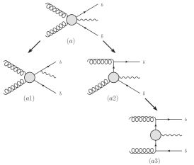
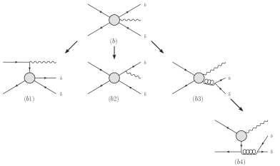
Figure 1: Representative parton-shower histories for $gg\to Zb\bar{b}$ (a) and $q\bar{q}\to Zb\bar{b}$ (b) matrix-element configurations. The gray blobs correspond to the irreducible core processes.

Some representative parton-shower histories, together with different core processes, are shown in Fig. 1. Figure 1 (a) is the starting point of the jet clustering procedure in $gg\to Zb\bar{b}$ configurations, which correspond to a leading-order prediction for $pp\to Zb\bar{b}$ in the four-flavor scheme. The first QCD clustering that can be performed on this configuration is the combination of a final-state (anti-)quark and an initial-state gluon, as indicated in Fig. 1 (a2). The second would then be the combination of the other final-state (anti-)quark and the second initial-state gluon, leading to Fig. 1 (a3). The core process in this case is $b\bar{b}\to Z$, which corresponds to the lowest-order hard matrix element in the five-flavor scheme. This example shows how the construction of parton-shower histories from hard matrix elements provides a natural matching of the two schemes. We will expand on this idea in Secs. III and IV. If the scale in the second clustering step, leading from Fig. 1 (a2) to Fig. 1 (a3) is lower than the scale in the first step, we speak of a violation of the scale hierarchy in the merging. In this case, the clustering procedure terminates after the first branching, and the core process is $gb\to Zb$ ($g\bar{b}\to Z\bar{b}$). It is also possible that the scale in the first clustering step exceeds all subsequently defined scales, including the scale associated with the core process. In this case, it may still be possible to perform an electroweak clustering, leading to Fig. 1 (a1), and defining the core process $gg\to b\bar{b}$. The correct probability for this would be given by electroweak evolution equations Bauer et al. (2017); Bauer and Webber (2019); Fornal et al. (2018), which are not yet implemented in standard parton showers. Therefore, one can choose to either neglect this clustering path (“exclusive clustering”), or allow it using ad-hoc clustering probabilities (“inclusive clustering”). Eventually, if no clustering can be performed due to the scale hierarchy, the core process may correspond to the starting configuration in Fig. 1 (a). Similar arguments apply to the possible parton-shower histories shown in Fig. 1 right. Again, the four-flavor scheme expression would correspond to Fig. 1 (b), and the analogue in the five-flavor scheme would be Fig. 1 (b4).

III Multi-jet merging in a variable flavor number scheme

In this section we describe our new algorithm, which combines a merged calculation in the five-flavor scheme with a prediction for heavy quark associated production. Both the merged and the heavy flavor prediction may be computed at leading order or at next-to-leading order QCD. The combination is achieved by means of a dedicated heavy flavor overlap removal. It acts on top of multi-jet merging algorithms and we call this technique fusing. We first explain it from a phenomenological point of view, using the example of $Z$+jets / $Zb\bar{b}$ production. The formal connection to the FONLL method will be established in Sec. IV.

The basic idea of the fusing approach is as follows:

1. Start with a merged simulation of the inclusive reaction, e.g. $Z$+jets and a calculation of heavy quark associated production, e.g. $Zb\bar{b}$.

2. Process the $Zb\bar{b}$ simulation as if it was part of the multi-jet merged computation, i.e. apply the clustering, the $\alpha_{s}$ reweighting and the Sudakov reweighting. The renormalization and factorization scales for the core process should be calculated using a custom scale definition, and the scales of all reconstructed splittings should be set to the transverse momenta in the branching Amati et al. (1980), including higher-order corrections to soft-gluon evolution Catani et al. (1991), cf. Sec. II. This part of the fused result will be called the direct component, as the final-state bottom quarks are generated in the fixed-order calculation.

3. Remove all final-state configurations from the five-flavor scheme merged simulation of $Z$+jets that have a parton-shower history which can also be generated in the reweighted $Zb\bar{b}$ computation. The remainder of the five-flavor scheme result may still contribute configurations with final-state bottom quarks. This part of the fused result will be called the fragmentation component.

4. Add the modified event samples to obtain the fused result.

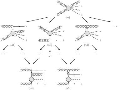
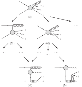
Figure 2: Example parton-shower histories for $gg\to Zb\bar{b}g$ (a), and $q\bar{q}\to Zb\bar{b}g$ (b). Depending on the clustering path, configurations (a5) and (b3) may be identified with a $Zb\bar{b}$ topology at leading order, while configurations (a4) and (b4) may not. At next-to-leading order, all configurations can be identified with a $Zb\bar{b}$ topology.

The removal of overlap between the $Z$+jets and the $Zb\bar{b}$ calculations is eventually achieved by both the Sudakov reweighting in step 2 and the event rejection in step 3. The application of Sudakov vetoes to $Zb\bar{b}$ restores the correct behavior of the direct component in those regions of phase space that feature a hierarchy between the hard scale and the b-quark mass. The event rejection in the $Z$+jets sample removes those final-state configurations which would otherwise be double counted. Algorithmically this rejection is performed as follows:

1. Create a combined evolution history, starting from the core process in the jet clustering, and ending with all final state particles produced either in the hard matrix element or by the shower.

2. Starting from the core process, find the first configuration where a $b\bar{b}$-pair appears in the final-state.

3. If there is no such configuration, keep the event. Otherwise, count the number of additional light partons $n_{\text{light}}$ (quarks or gluons) in the final state of this configuration. This corresponds to the number of hard emissions before the $b\bar{b}$-pair production according to the ordering imposed by the cluster (shower) algorithm. At leading order, discard the event if $n_{\text{light}}=0$. At next-to-leading order, discard the event if $n_{\text{light}}\leq 1$.

Typical parton-shower histories for candidate $Z$+jets events with gluon or quark initial states are shown in Fig. 2. If the clustering leading to configurations (a5) / (b3) proceeds along (a3) / (b1), the scale associated with the gluon emission is the smallest in the process. The configuration can then be identified with a $Zb\bar{b}$ topology, and the event will be discarded. If the clustering proceeds along (a2) / (b2), the treatment depends on whether the fusing is performed at leading or at next-to-leading order. At leading order the configuration cannot be identified with a $Zb\bar{b}$ topology, and the event will be kept. At next-to-leading order, the configuration corresponds to a real-emission configuration, and the event will be discarded. Figure 2 (a4) / (b4) displays a parton-shower history that does not have a counterpart in the heavy-flavor result at leading order, such that the corresponding event would be kept irrespective of the scale hierarchy. At next-to-leading order, the event would be discarded. The extension to histories with more partons in the final state is straightforward and will lead to configurations that contribute to the fragmentation component also in the next-to-leading order case.

Special care has to be taken when dealing with unordered configurations. They arise when the clustering algorithm can not reconstruct a strictly $k_{T}$-ordered history leading to a $pp\to Z$ core process (cf. Sec. II). In such cases, the clustering can either stop with a $2\rightarrow n$ core process, or continue by allowing to violate the scale hierarchy. Both variants can be used for the fusing algorithm as long as all components and all parton multiplicities are treated identically. In this work we restrict ourselves to a fully-ordered clustering algorithm.

IV Relation to the FONLL method

This section will establish the relation between our merging algorithm and the FONLL method Forte et al. (2015, 2016). In the FONLL technique, the cross section of the combined event sample is generated as

$$\sigma^{\rm FONLL}=\sigma^{(5)}-\sigma^{(4),(0)}+\sigma^{(4)}\;,$$ (1)

where $\sigma^{(5)}$ and $\sigma^{(4)}$ are the cross sections in the five- and four-flavor scheme, respectively, and $\sigma^{(4),(0)}$ is the four-flavor scheme result in the limit $m_{b}\to 0$. Eventually, all results should only depend on the PDFs and strong coupling in the five-flavor scheme. Formally, this is achieved by writing the cross section as

$$\sigma^{(4)}=\int dx_{1}\int dx_{2}\,\sum_{ij=q,g}f_{i}^{(5)}(x_{1},Q^{2})f_{j}^{(5)}(x_{2},Q^{2})\,B_{ij}\left(x_{1}x_{2},\alpha_{s}^{(5)}(Q^{2}),\frac{Q^{2}}{m_{b}^{2}}\right)\;.$$ (2)

The hard coefficients $B_{ij}$ can then be expanded in powers of the strong coupling as

$$B_{ij}\left(\tau,\alpha_{s}^{(5)}(Q^{2}),\frac{Q^{2}}{m_{b}^{2}}\right)=\sum_{n=2}\bigg{(}\frac{\alpha_{s}^{(5)}(Q^{2})}{2\pi}\bigg{)}^{n}B_{ij}^{(n)}\left(\tau,\frac{Q^{2}}{m_{b}^{2}}\right)\;,$$ (3)

and are determined such that the four-flavor scheme result in terms of four-flavor PDFs is eventually recovered at the target accuracy given by the upper limit of the sum.

The coefficients $\sigma^{(4),(0)}$, needed for removal of the overlap between the fully massive and the massless calculation, can be extracted from the five-flavor scheme result Forte et al. (2016) by expressing the b-quark PDF up to $\mathcal{O}(\alpha_{s})$ in terms of the four-flavor scheme light quark and gluon PDFs using the matching coefficients from Buza et al. (1998), and subsequently re-expressing the result in terms of five-flavor scheme PDFs and $\alpha_{s}$ Forte et al. (2010). The result is

$$\begin{split}f_{b}^{(5)}(x,Q^{2})=&\;\frac{\alpha_{s}(\mu_{R}^{2})}{2\pi}\int_{x}^{1}\frac{dz}{z}A_{gb}^{(1)}(z,L)f_{g}^{(5)}\left(\frac{x}{z},Q^{2}\right)\\ &\;+\frac{\alpha_{s}^{2}(\mu_{R}^{2})}{(2\pi)^{2}}\int_{x}^{1}\frac{dz}{z}\left[\,A_{gb}^{(2)}(z,L)f_{g}^{(5)}\left(\frac{x}{z},Q^{2}\right)+A_{\Sigma b}^{(2)}(z,L)f_{\Sigma}^{(5)}\left(\frac{x}{z},Q^{2}\right)\,\right]\;,\end{split}$$ (4)

where $L=\ln Q^{2}/m_{b}^{2}$ and $f_{\Sigma}=\sum_{a=q,\bar{q}}f_{a}(x,Q^{2})$. We can now use the $\mathcal{O}(\alpha_{s}^{n})$ five-flavor scheme partonic cross sections $\hat{\sigma}^{(n)}$ to define the massless limit of the coefficient functions $B^{(n)}$. In the processes of interest to us the partonic cross section is invariant under exchange of $b$ and $\bar{b}$. The $\mathcal{O}(\alpha_{s}^{2})$ terms are then given by

$$\begin{split}B_{q\bar{q}}^{(0),(2)}\left(\tau,\frac{Q^{2}}{m_{b}^{2}}\right)=&\;\hat{\sigma}_{q\bar{q}}^{(2)}(\tau)+2\int_{\tau}^{1}\frac{dz}{z}A_{qq,b}^{(2)}(z,L)\,\hat{\sigma}_{q\bar{q}}^{(0)}\Big{(}\frac{\tau}{z}\Big{)}\;,\\ B_{gg}^{(0),(2)}\left(\tau,\frac{Q^{2}}{m_{b}^{2}}\right)=&\;\hat{\sigma}_{gg}^{(2)}(\tau)+4\int_{\tau}^{1}\frac{dz}{z}A_{gb}^{(1)}(z,L)\,\hat{\sigma}_{gb}^{(1)}\left(\frac{\tau}{z}\right)+2\int_{\tau}^{1}\frac{dz}{z}\int_{z}^{1}\frac{dy}{y}A_{gb}^{(1)}(y,L)A_{gb}^{(1)}\Big{(}\frac{z}{y},L\Big{)}\,\hat{\sigma}_{b\bar{b}}^{(0)}\Big{(}\frac{\tau}{z}\Big{)}\;.\end{split}$$ (5)

The $\mathcal{O}(\alpha_{s}^{3})$ terms are given by

$$\begin{split}&B_{gg}^{(0),(3)}\left(\tau,\frac{Q^{2}}{m_{b}^{2}}\right)=\int_{\tau}^{1}\frac{dz}{z}\bigg{[}\,4A_{gb}^{(1)}(z,L)\,\hat{\sigma}_{gb}^{(2)}\left(\frac{\tau}{z},L\right)+4A_{gb}^{(2)}(z,L)\,\hat{\sigma}_{gb}^{(1)}\left(\frac{\tau}{z},L\right)\bigg{]}\\ &\qquad+\int_{\tau}^{1}\frac{dz}{z}\int_{z}^{1}\frac{dy}{y}\bigg{[}\,2A_{gb}^{(1)}(y,L)A_{gb}^{(1)}\Big{(}\frac{z}{y},L\Big{)}\,\hat{\sigma}_{b\bar{b}}^{(1)}\left(\frac{\tau}{z}\right)+4A_{gb}^{(2)}(y,L)A_{gb}^{(1)}\Big{(}\frac{z}{y},L\Big{)}\,\hat{\sigma}_{b\bar{b}}^{(0)}\Big{(}\frac{\tau}{z}\Big{)}\bigg{]}\;,\\ &B_{gq}^{(0),(3)}\left(\tau,\frac{Q^{2}}{m_{b}^{2}}\right)=\;\int_{\tau}^{1}\frac{dz}{z}\,\bigg{[}2A_{gb}^{(1)}(z,L)\,\hat{\sigma}_{qb}^{(2)}\left(\frac{\tau}{z},L\right)+2A_{\Sigma b}^{(2)}(z,L)\,\hat{\sigma}_{gb}^{(1)}\left(\frac{\tau}{z},L\right)\bigg{]}\\ &\qquad+\int_{\tau}^{1}\frac{dz}{z}\int_{z}^{1}\frac{dy}{y}\,2A_{\Sigma b}^{(2)}(y,L)A_{gb}^{(1)}\Big{(}\frac{z}{y},L\Big{)}\,\hat{\sigma}_{b\bar{b}}^{(0)}\left(\frac{\tau}{z}\right)+\int_{\tau}^{1}\frac{dz}{z}\,2A_{qq,b}^{(2)}(z,L)\,\hat{\sigma}_{gq}^{(1)}\left(\frac{\tau}{z},L\right)\;,\\ &B_{q\bar{q}}^{(0),(3)}\left(\tau,\frac{Q^{2}}{m_{b}^{2}}\right)=\int_{\tau}^{1}\frac{dz}{z}\,2A_{qq,b}^{(2)}(z,L)\,\hat{\sigma}_{q\bar{q}}^{(1)}\left(\frac{\tau}{z},L\right)\;.\\ \end{split}$$ (6)

The matching coefficients in Eq. (4) can be expanded in a power series in $L$ as

$$\begin{split}A_{gb}^{(1)}(z,L)=&\;a_{gb}^{(1,1)}(z)L\;,\\ A_{gb}^{(2)}(z,L)=&\;a_{gb}^{(2,2)}(z)L^{2}+a_{gb}^{(2,1)}(z)L+a_{gb}^{(2,0)}(z)\;,\\ A_{\Sigma b}^{(2)}(z,L)=&\;a_{\Sigma b}^{(2,2)}(z)L^{2}+a_{\Sigma b}^{(2,1)}(z)L+a_{\Sigma b}^{(2,0)}(z)\;,\\ A_{qq,b}^{(2)}(z,L)=&\;a_{qq,b}^{(2,2)}(z)L^{2}+a_{qq,b}^{(2,1)}(z)L+a_{qq,b}^{(2,0)}(z)\;.\end{split}$$ (7)

In the parton-shower approach, each logarithm $L$ arises from integrating Eq. (31) over $\ln t$ from $m_{b}^{2}$ to $Q^{2}$. By comparing to Eq. (4) we find that $A_{gb}^{(1)}(z,L)=P_{gq}(z)L$. We will comment on the remaining coefficients in Sec. IV.2. The non-logarithmic terms, $a^{(2,0)}(z)$, are needed only for matching beyond NLL accuracy and can therefore be ignored in our approach. The leading and sub-leading logarithmic terms can be derived from renormalization and collinear mass factorization of the operator matrix elements for heavy quark production Buza et al. (1996). They take the simple form

$$\begin{split}a_{gb}^{(1,1)}(z)=&\;P_{gq}(z)\;,\\ a_{gb}^{(2,2)}(z)=&\;\frac{1}{2}\int_{z}^{1}\frac{dx}{x}P_{gq}(x)P_{qq}\left(\frac{z}{x}\right)+\beta_{0}\,P_{gq}(z)-\frac{1}{2}\int_{z}^{1}\frac{dx}{x}P_{gg}(x)P_{gq}\left(\frac{z}{x}\right)\;,&a_{gb}^{(2,1)}(z)=&\;P_{gq}^{(1)}(x)\;,\\ a_{\Sigma b}^{(2,2)}(z)=&\;-\frac{1}{2}\int_{z}^{1}\frac{dx}{x}P_{qg}(x)P_{gq}\left(\frac{z}{x}\right)\;,&a_{\Sigma b}^{(2,1)}(z)=&\;P_{qq}^{S,(1)}(x)\;,\\ a_{qq,b}^{(2,2)}(z)=&\;-\frac{1}{2}\,\beta_{0,b}\,P_{qq}(z)\;,&a_{qq,b}^{(2,1)}(z)=&\;P_{qq,Q}^{V,(1)}(x)\;.\end{split}$$ (8)

The leading-order and relevant next-to-leading order splitting functions entering Eqs. (8) are given in App. B. The negative term in $a_{gb}^{(2,2)}(z)$ and the coefficient $a_{\Sigma b}^{(2,2)}(z)$ are collinear mass factorization counterterms that arise from the different number of quark flavors in the infrared and the ultraviolet regime Buza et al. (1996, 1998).

IV.1 Leading Order and Leading Logarithmic Accuracy

In order to prove that the heavy flavor overlap removal algorithm proposed in this publication amounts to a variant of the FONLL method we need to show that the removal of events from the five-flavor sample as proposed in Sec. III is equivalent to the subtraction of $\sigma^{(4),(0)}$ in the FONLL technique. We will start at leading order and leading logarithmic accuracy and comment on next-to-leading order and next-to-leading logarithmic accuracy in the next section.

The simplest configurations are $\hat{\sigma}^{(2)}_{q\bar{q}}$ and $\hat{\sigma}^{(2)}_{gg}$ in Eq. (5). They correspond to removal of the double-real radiative corrections to the $b\bar{b}\to Z$ process, which have a counterpart in the four-flavor scheme. Note that, in the notation of Eq. (5), $\hat{\sigma}^{(2)}_{q\bar{q}}$ and $\hat{\sigma}^{(2)}_{gg}$ are integrated over the double-real radiative phase space and combined with the renormalized virtual corrections and collinear mass factorization counterterms, which renders both $\hat{\sigma}^{(2)}_{q\bar{q}}$ and $\hat{\sigma}^{(2)}_{gg}$ individually finite. In the $\overline{\rm MS}$ scheme, the factorization scale dependent remainder combines with the PDF evolution to give the second and third expression on the right-hand side of Eq. (5). In a multi-jet merging approach, no singularities arise because we effectively use a cutoff regulator for collinear mass singularities that is defined by the jet cuts. For $gg$ initial states we obtain

$$\begin{split}B_{gg,\rm MEPS}^{(0),(2)}\left(\tau,\frac{Q^{2}}{m_{b}^{2}}\right)=&\;\int{\rm d}\Phi_{2}\,\frac{{\rm d}\hat{\sigma}_{gg}^{(2)}(\tau)}{{\rm d}\Phi_{2}}\,\Theta(Q_{1}-Q_{\rm cut})\Theta(Q_{2}-Q_{\rm cut})\\ &+4\int_{m_{b}^{2}}^{Q^{2}}\!\!\frac{{\rm d}t}{t}\int_{\tau}^{1}\frac{dz}{z}P_{gq}(z)\,\int{\rm d}\Phi_{1}\,\frac{{\rm d}\hat{\sigma}_{gb}^{(1)}\left(\tau/z\right)}{{\rm d}\Phi_{1}}\,\Theta(Q_{1}-Q_{\rm cut})\Theta(Q_{\rm cut}-Q_{2})\\ &+2\int_{m_{b}^{2}}^{Q^{2}}\!\!\frac{{\rm d}t}{t}\int_{\tau}^{1}\frac{dz}{z}\int_{m_{b}^{2}}^{t}\!\!\frac{{\rm d}t^{\prime}}{t^{\prime}}\int_{z}^{1}\frac{dy}{y}P_{gq}(y)P_{gq}\Big{(}\frac{z}{y}\Big{)}\,\hat{\sigma}_{b\bar{b}}^{(0)}\Big{(}\frac{\tau}{z}\Big{)}\,\Theta(Q_{\rm cut}-Q_{1})\\ \approx&\;B_{gg}^{(0),(2)}\left(\tau,\frac{Q^{2}}{m_{b}^{2}}\right)\bigg{|}_{\;\rm LL}\;,\end{split}$$ (9)

where the subscript ${\rm LL}$ indicates leading logarithmic accuracy. The scales $Q_{1}$ and $Q_{2}$ denote the jet resolution in the final and next-to-final clustering of the merging algorithm, while $Q_{\rm cut}$ stands for the merging scale. The $\Theta$-functions represent the phase-space partitioning in the merging procedure with at least two jets in addition to the production of the inclusive final state in the five-flavor scheme. The last approximation is valid if the merging cut is small enough that below it we can factorize $\hat{\sigma}_{gg}^{(2)}$ and $\hat{\sigma}_{gb}^{(1)}$ into $\hat{\sigma}_{b\bar{b}}^{(0)}$ and $P_{gb}$, and if we can ignore the finite remainder of the virtual corrections included in Eq. (5). The subtraction of $\sigma^{(4),(0)}$ from $\sigma^{(5)}$ in Eq. (1) can therefore be achieved by using the algorithm in Sec. III. In the case of $gg$ initial states it proceeds as follows:

1. Construct a parton-shower history according to the multi-jet merging procedure, perform the parton shower and add any splittings that were generated to the history

2. Starting at the core interaction identified in the merging, trace the parton-shower history. Veto the event if

   1. the core process is $b\bar{b}\to Z$, followed by an initial-state $g\to b\bar{b}$ and $g\to\bar{b}b$ branching

   2. the core process is $gb\to Zb$ ($g\bar{b}\to Z\bar{b}$), followed by an initial-state $g\to b\bar{b}$ ($g\to\bar{b}b$) branching

   3. the core process is $gg\to Zb\bar{b}$

The solution is similar for quark initial states, only the sequence of parton-shower splittings differs. The multi-jet merged expression reads

$$\begin{split}B_{q\bar{q},\rm MEPS}^{(0),(2)}\left(\tau,\frac{Q^{2}}{m_{b}^{2}}\right)=&\;\int{\rm d}\Phi_{2}\,\frac{{\rm d}\hat{\sigma}_{q\bar{q}}^{(2)}(\tau)}{{\rm d}\Phi_{2}}\,\Theta(Q_{2}-Q_{\rm cut})\Theta(Q_{1}-Q_{\rm cut})\\ &+\int_{m_{b}^{2}}^{Q^{2}}\!\!\frac{{\rm d}t}{t}\int_{0}^{1}{\rm d}z\,z\,P_{gq}(z)\,\int{\rm d}\Phi_{1}\,\frac{{\rm d}\hat{\sigma}_{q\bar{q}}^{(1)}\left(\tau\right)}{{\rm d}\Phi_{1}}\,\Theta(Q_{1}-Q_{\rm cut})\Theta(Q_{\rm cut}-Q_{2})\\ &+2\int_{m_{b}^{2}}^{Q^{2}}\!\!\frac{{\rm d}t}{t}\int_{\tau}^{1}\frac{dz}{z}\int_{m_{b}^{2}}^{t}\!\!\frac{{\rm d}t^{\prime}}{t^{\prime}}\int_{0}^{1}{\rm d}y\,y\,P_{gq}(y)P_{qq}(z)\,\hat{\sigma}_{b\bar{b}}^{(0)}\Big{(}\frac{\tau}{z}\Big{)}\,\Theta(Q_{\rm cut}-Q_{1})\\ \approx&\;B_{q\bar{q}}^{(0),(2)}\left(\tau,\frac{Q^{2}}{m_{b}^{2}}\right)\bigg{|}_{\;\rm LL}\;.\end{split}$$ (10)

The origin of $a_{qq,b}^{(2,2)}(z)$ contained in $B_{q\bar{q}}^{(0),(2)}\big{|}_{\;\rm LL}$ is explained in Sec. IV.2.

IV.2 Next-to-Leading Order and Next-to-Leading Logarithmic Accuracy

In order to achieve next-to-leading logarithmic accuracy according to the FONLL method, the parton shower employed in the merging must implement all coefficient functions in Eq. (8). We start with the $\beta_{0}$ dependent contribution to $a_{gb}^{(2,2)}(z)$. Making use of the expansion of the strong coupling in the four-flavor scheme to $\mathcal{O}(\alpha_{s})$,

$$\alpha_{s}(m_{b}^{2})=\alpha_{s}\left[\,1+\frac{\alpha_{s}}{2\pi}\,\beta_{0}\,L\,\right]\;,$$ (11)

this term can either be implemented explicitly, or absorbed into the scale choice connected to the evaluation of $a_{gb}^{(1,1)}(z)$. In the latter case, the strong coupling in initial-state $g\to b\bar{b}$ splittings should be computed at $m_{b}^{2}$. Because we use a strong coupling in the five-flavor scheme, an additional counterterm of the form $\alpha_{s}/(2\pi)\beta_{0,b}L$ will then be required.

The coefficients $a^{(2,2)}(z)$ can be expressed in the parton-shower formalism as the convolution of $a_{gb}^{(1,1)}(z)$ with the emission and no-emission probability of the parton shower, expanded to second order in the strong coupling and integrated over the evolution parameter from $m_{b}^{2}$ to $Q^{2}$. To show this, we employ the correspondence between inclusive and exclusive parton evolution summarized in App. A. Making use of Eq. (32) and the boundary condition $f_{b}(x,m_{b}^{2})=0$, a single step in the parton-shower backward evolution, generating a resolved $g\to b\bar{b}$ transition at scale $Q^{2}$ can be written formally as

$$f_{b}(x,Q^{2})=\int_{m_{b}^{2}}^{Q^{2}}\!\frac{{\rm d}t}{t}\,\frac{\alpha_{s}}{2\pi}\int_{x}^{1}\frac{{\rm d}z}{z}\,P_{gq}(z)\,f_{g}\Big{(}\frac{x}{z},t\Big{)}\;.$$ (12)

Upon expansion to $\mathcal{O}(\alpha_{s})$, we obtain the leading-order coefficient of Eq. (4). To reconstruct the first term in $a_{gb}^{(2,2)}(z)$, we need to account for a second step in the parton-shower evolution, preceding the $g\to b\bar{b}$ transition. This gives

$$\begin{split}&\int_{m_{b}^{2}}^{Q^{2}}\!\frac{{\rm d}t}{t}\,\frac{\alpha_{s}}{2\pi}\int_{x}^{1-\varepsilon}\frac{{\rm d}z}{z}\left[P_{gq}(z)\,\Delta_{q}(t,Q^{2})+\int_{t}^{Q^{2}}\!\frac{{\rm d}\bar{t}}{\bar{t}}\,\frac{\alpha_{s}}{2\pi}\int_{z}^{1-\varepsilon^{\prime}}\frac{{\rm d}y}{y}P_{gq}\Big{(}\frac{z}{y}\Big{)}\,\hat{P}_{qq}(y)\,\Delta_{q}(\bar{t},Q^{2})\right]\,f_{g}\Big{(}\frac{x}{z},t\Big{)}\;.\end{split}$$ (13)

Subtracting the leading-order term in Eq. (12), and expanding to second order in the strong coupling, we can write

$$\frac{\alpha_{s}^{2}}{(2\pi)^{2}}\int_{m_{b}^{2}}^{Q^{2}}\!\frac{{\rm d}t}{t}\int_{x}^{1-\varepsilon}\frac{{\rm d}z}{z}\int_{t}^{Q^{2}}\frac{{\rm d}\bar{t}}{\bar{t}}\left[-P_{gq}(z)\sum_{a=q,g}\int_{0}^{1-\varepsilon^{\prime}}\!\!{\rm d}\zeta\,\zeta\,\hat{P}_{qa}(\zeta)+\int_{z}^{1-\varepsilon^{\prime}}\frac{{\rm d}y}{y}\,P_{gq}\Big{(}\frac{z}{y}\Big{)}\,\hat{P}_{qq}(y)\right]\,f_{g}\Big{(}\frac{x}{z},Q^{2}\Big{)}\;.$$ (14)

Using Eq. (26) and (27), and taking the limit $\varepsilon,\varepsilon^{\prime}\to 0$, gives

$$\frac{\alpha_{s}^{2}}{(2\pi)^{2}}\int_{m_{b}^{2}}^{Q^{2}}\!\frac{{\rm d}t}{t}\int_{x}^{1}\frac{{\rm d}z}{z}\int_{t}^{Q^{2}}\frac{{\rm d}\bar{t}}{\bar{t}}\int_{z}^{1}\frac{{\rm d}y}{y}\,P_{gq}\Big{(}\frac{z}{y}\Big{)}\,P_{qq}(y)\,f_{g}\Big{(}\frac{x}{z},Q^{2}\Big{)}\;.$$ (15)

Finally, we make use of the fact that at $\mathcal{O}(\alpha_{s}^{2})$ there is no further dependence on $t$ and $\bar{t}$. Integrating them out we obtain the contribution of the first term in $a_{gb}^{(2,2)}(z)$ to Eq. (4)

$$\frac{\alpha_{s}^{2}}{(2\pi)^{2}}\frac{L^{2}}{2}\int_{x}^{1}\frac{{\rm d}z}{z}\int_{z}^{1}\frac{{\rm d}y}{y}\,P_{gq}\Big{(}\frac{z}{y}\Big{)}\,P_{qq}(y)\,f_{g}\Big{(}\frac{x}{z},Q^{2}\Big{)}\;.$$ (16)

The coefficient $a_{\Sigma b}^{(2,2)}(z)$ and the final term in $a_{gb}^{(2,2)}(z)$ are derived in a similar way. The difference compared to the previous case is that the hierarchy between $m_{b}^{2}$ and $Q^{2}$ is ill-defined, because the second branching happens at smaller scales than the $g\to b\bar{b}$ transition. The complete parton-shower expression for the splitting kernel in $a_{gb}^{(1,1)}(z)$ and one step of the subsequent evolution reads

$$\begin{split}&\int_{m_{b}^{2}}^{Q^{2}}\!\frac{{\rm d}t}{t}\,\frac{\alpha_{s}}{2\pi}\int_{x}^{1-\varepsilon}\frac{{\rm d}z}{z}\left[P_{gq}(z)\,\Delta_{g}(q^{2},t)+\sum_{a=q,g}\int_{q^{2}}^{t}\frac{{\rm d}\bar{t}}{\bar{t}}\frac{\alpha_{s}}{2\pi}\int_{z}^{1-\varepsilon^{\prime}}\frac{{\rm d}y}{y}\hat{P}_{ag}\Big{(}\frac{z}{y}\Big{)}\,P_{gq}(y)\,\Delta_{g}(\bar{t},t)\right]\,f_{g}\Big{(}\frac{x}{z},t\Big{)}\;.\end{split}$$ (17)

Note that we have introduced an auxiliary scale, $q^{2}$, in order to perform the integral over the second branching. Subtracting the leading-order term in Eq. (12), and expanding to second order in the strong coupling, we can write

$$\begin{split}\frac{\alpha_{s}^{2}}{(2\pi)^{2}}\int_{m_{b}^{2}}^{Q^{2}}\!\frac{{\rm d}t}{t}\int_{x}^{1-\varepsilon}\frac{{\rm d}z}{z}\int^{t}_{q^{2}}\frac{{\rm d}\bar{t}}{\bar{t}}\Bigg{[}&-P_{gq}(z)\sum_{a=q,g}\int_{0}^{1-\varepsilon^{\prime}}\!\!{\rm d}\zeta\,\zeta\,\hat{P}_{ga}(\zeta)\,f_{g}\Big{(}\frac{x}{z},Q^{2}\Big{)}\\ &+\sum_{a=q,g}\int_{z}^{1-\varepsilon^{\prime}}\frac{{\rm d}y}{y}\,\hat{P}_{ag}\Big{(}\frac{z}{y}\Big{)}\,P_{gq}(y)\,f_{a}\Big{(}\frac{x}{z},Q^{2}\Big{)}\Bigg{]}\;.\end{split}$$ (18)

Using again Eq. (26) and (27), taking the limit $\varepsilon,\varepsilon^{\prime}\to 0$, and integrating over $t$ and $\bar{t}$, we obtain

$$\frac{\alpha_{s}^{2}}{(2\pi)^{2}}\,\frac{L}{2}\ln\frac{m_{b}^{2}Q^{2}}{q^{4}}\int_{x}^{1}\frac{{\rm d}z}{z}\sum_{a=q,g}\int_{z}^{1}\frac{{\rm d}y}{y}\,P_{ag}\Big{(}\frac{z}{y}\Big{)}\,P_{gq}(y)\,f_{a}\Big{(}\frac{x}{z},Q^{2}\Big{)}\;.$$ (19)

Note that $q^{2}$ plays the role of the collinear mass factorization scale, while $Q^{2}$ corresponds to the UV renormalization scale. In the parton-shower approach, the two are strictly ordered, as the second branching cannot take place before the first one. In a fixed-order computation, we can instead set $q=Q$. This corresponds to treating the UV renormalization and collinear mass factorization counterterms in Eqs. (3.15) and (3.20) of Buza et al. (1996) on the same footing, which is eventually mandated by the choice to set $\epsilon_{\rm UV}=\epsilon_{\rm IR}$. Using the same scheme in Eq. (19), i.e. setting $q\to Q$, we obtain the contribution of $a_{\Sigma b}^{(2,2)}(z)$ and the final term in $a_{gb}^{(2,2)}(z)$ to Eq. (4)

$$-\frac{\alpha_{s}^{2}}{(2\pi)^{2}}\,\frac{L^{2}}{2}\int_{x}^{1}\frac{{\rm d}z}{z}\sum_{a=q,g}\int_{z}^{1}\frac{{\rm d}y}{y}\,P_{ag}\Big{(}\frac{z}{y}\Big{)}\,P_{gq}(y)\,f_{a}\Big{(}\frac{x}{z},Q^{2}\Big{)}\;.$$ (20)

The coefficient $a_{qq,b}^{(2,2)}(z)$ can be derived in a similar fashion. The difference compared to $a_{\Sigma b}^{(2,2)}(z)$ lies in the fact that the phase space for the final-state branching of the intermediate gluon into $b\bar{b}$ can be integrated out, leading to the coefficient $-\beta_{0,b}$. The complete parton-shower expression reads

$$\begin{split}&\int_{m_{b}^{2}}^{Q^{2}}\!\frac{{\rm d}t}{t}\,\frac{\alpha_{s}}{2\pi}\sum_{a=b,\bar{b}}\int_{0}^{1-\varepsilon^{\prime}}{\rm d}y\,y\,P_{ga}(y)\Bigg{[}\Delta_{q}(t,Q^{2})+\int^{Q^{2}}_{t}\frac{{\rm d}\bar{t}}{\bar{t}}\frac{\alpha_{s}}{2\pi}\int_{x}^{1-\varepsilon}\frac{{\rm d}z}{z}P_{qq}(z)\Delta_{q}(\bar{t},Q^{2})\Bigg{]}\,f_{g}\Big{(}\frac{x}{z},t\Big{)}\;.\end{split}$$ (21)

This can be expanded to second order in the strong coupling as in Eqs. (14) and (18). Taking the limit $\varepsilon,\varepsilon^{\prime}\to 0$, and integrating over $t$ and $\bar{t}$, we obtain the contribution of $a_{qq,b}^{(2,2)}(z)$ to Eq. (4)

$$\frac{\alpha_{s}^{2}}{(2\pi)^{2}}\,\frac{L^{2}}{2}\,\bigg{(}\sum_{a=b,\bar{b}}\int_{0}^{1}{\rm d}y\,y\,P_{ga}(y)\bigg{)}\int_{x}^{1}\frac{{\rm d}z}{z}\,P_{qq}(z)\,f_{g}\Big{(}\frac{x}{z},t\Big{)}=-\frac{\alpha_{s}^{2}}{(2\pi)^{2}}\,\frac{L^{2}}{2}\,\beta_{0,b}\int_{x}^{1}\frac{{\rm d}z}{z}\,P_{qq}(z)\,f_{g}\Big{(}\frac{x}{z},t\Big{)}\;.$$ (22)

Combining the parton-shower effects leading to Eqs. (16), (20), (22) and (11), we obtain all double logarithmic coefficients in Eq. (8). The single logarithmic coefficients are not reproduced by a standard parton shower and must be implemented separately. In the case of $a_{\Sigma b}^{(2,1)}$ and $a_{qq,b}^{(2,1)}$ this can be achieved using the algorithm derived in Höche and Prestel (2017). Although a complete Monte-Carlo implementation has not yet been presented for $a_{gb}^{(2,1)}$, it is clear that it can be constructed using the techniques of Höche and Prestel (2017) and Dulat et al. (2018). In the foreseeable future it will therefore be possible to achieve next-to-leading logarithmic accuracy according to the FONLL classification by using our approach.

In order to achieve next-to-leading order accuracy according to the FONLL method, we must reconstruct the coefficient functions in Eq. (6). The modification of the leading-order result, Eq. (5), by the multi-jet merging procedure has already been discussed in Sec. IV.1. In complete analogy, the terms proportional to $\hat{\sigma}_{b\bar{b}}$ in Eq. (6) are modified by $\Theta(Q_{\rm cut}-Q_{1})\Theta(Q_{\rm cut}-Q_{2})$ in the merging, while the terms proportional to $\hat{\sigma}_{gb}$ and $\hat{\sigma}_{qb}$ are modified by $\Theta(Q_{1}-Q_{\rm cut})\Theta(Q_{\rm cut}-Q_{2})$. It remains to adjust the result for the fact that the four-flavor scheme coefficients in the perturbative expansion are determined using a strong coupling in the five-flavor scheme. We use Eqs. (8) and (9) of Forte et al. (2016) to correct this mismatch. Technically this is achieved by modifying the event weight $w$ of four-flavor scheme $S$-events with $gg$ or $q\bar{q}$ initial-state as

$$\begin{split}w_{q\bar{q}}^{\text{new}}=&w_{q\bar{q}}\left(1-\frac{4}{3}T_{R}\ln\frac{\mu_{R}^{2}}{Q^{2}}\frac{w^{\text{Born}}}{w^{\text{ME}}}\right)\\ w_{gg}^{\text{new}}=&w_{gg}\left(1-\frac{4}{3}T_{R}\ln\frac{\mu_{R}^{2}}{m_{b}^{2}}\frac{w^{\text{Born}}}{w^{\text{ME}}}\right)\;,\\ \end{split}$$ (23)

where $w^{\text{Born}}$ and $w^{\text{ME}}$ are the matrix-element weights of the Born contribution and the full $S$-event, respectively.

V Results

The algorithm described in Sec. III has been implemented in the Sherpa event generator in full generality, and will be investigated in the following for the example of heavy flavor production in association with a $Z$ boson.

As argued in Section IV.2, a NLO-accurate parton shower would be needed to fully match the next-to-leading logarithmic accuracy of the FONLL method. Such a shower is not available yet but recent studies indicate that the central predictions provided by it should be close to the LO result Höche and Prestel (2017); Dulat et al. (2018). We thus base our new approach on the established MEPS@NLO algorithm, which we have extended to provide the necessary fully-ordered clustering and combined parton-shower history for Sherpa version 2.2.7. The event filter for the overlap removal described in Sec. III and the counter-terms described in Eq. (23) are implemented as user hooks. The event filter can either directly be used to veto events or store the veto information as alternative event weight. This allows to produce a $Z$+jets sample which is usable both standalone, or within a fused prediction by applying the corresponding event weight and adding a dedicated sample only for the direct component.

In the next sections we compare predictions obtained by the newly developed algorithm against existing predictions in the 5FS and the 4FS. In all of them the matrix elements are generated using Sherpa’s internal matrix element generators Amegic++ Krauss et al. (2002) and Comix Gleisberg and Höche (2008) for tree-level diagrams. Virtual diagrams are interfaced from OpenLoops 1.3.1 Cascioli et al. (2012), using CutTools Ossola et al. (2008) and OneLoop van Hameren (2011).

In the 5FS prediction and for the fragmentation component, matrix elements are calculated for $pp\rightarrow\ell^{+}\ell^{-}+0,1,2j\text{@NLO}+3j\text{@LO}$. Here, $\ell^{+},\ell^{-}$ refers to either electrons or muons and $j$ to a well separated parton. The merging cut $Q_{\text{cut}}$ is set to $20~{}\text{G$\text{e}\mspace{-0.8mu}\text{V}$}$ if not stated otherwise. The direct component and the standalone 4FS prediction are based on $pp\rightarrow\ell^{+}\ell^{-}b\bar{b}$ matrix elements at next-to-leading order, matched to the parton shower using the formalism in Höche et al. (2012).

For both components of the fusing approach, and for the standalone 5FS and 4FS predictions, all scales are evaluated according to the METS scheme with inclusive clustering. In all predictions except for the standalone 4FS prediction the clustering is required to be fully ordered. The factorization and (where applicable) renormalization scales in the core process are evaluated according to

$$\mu^{2}_{\text{core}}=\begin{cases}m^{2}_{\ell\ell}&\text{for $Z$},\\ \tfrac{1}{4}m^{2}_{\perp,\ell\ell}&\text{for $Zj$},\\ \tfrac{1}{4}\tfrac{-1}{1/\hat{s}+1/\hat{t}+1/\hat{u}}&\text{for jet+jet},\\ \tfrac{1}{4}\bigl{(}m_{\perp,\ell\ell}~{}+\sum_{\text{jets}}m_{\perp,\text{jet}}\bigr{)}^{2}&\text{for unordered $Z$+jets.}\\ \end{cases}$$ (24)

We use the NNPDF3.0 set Ball et al. (2015) at NNLO with five active flavors for both components of the fusing approach and for the 5FS prediction, and with four active flavors for the 4FS prediction. These PDF sets are interfaced to Sherpa using LHAPDF Buckley et al. (2015). We use the CS-Shower Schumann and Krauss (2008) as implemented in Sherpa with two minor modifications. Firstly, the strong coupling in $g\to b\bar{b}$ splittings is evaluated at the virtuality of the intermediate parton, to account for the fact that there is no soft gluon emission, and therefore no higher-order corrections enhanced by $\alpha_{s}/(2\pi)\beta_{0}\ln k_{T}^{2}/Q^{2}$. Secondly, we choose the evolution variables of Scheme 1 in Hoeche et al. (2014), but we add the squared masses of the final-state partons in the branching. The default multiple interactions Sjöstrand and van Zijl (1987); *Alekhin:2005dx and hadronization models Winter et al. (2004) implemented in Sherpa are employed in all simulations. Analyses of the event samples are performed within the Rivet framework Buckley et al. (2013). Scale variations ($\mu_{\text{F}}$, $\mu_{\text{R}}$) are studied using the on-the-fly-variation method as implemented in Sherpa Bothmann et al. (2016).

V.1 Validation in inclusive $Z$ phase space

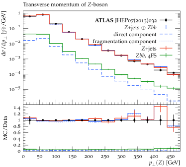
(a) The transverse momentum of the $Z$ boson.

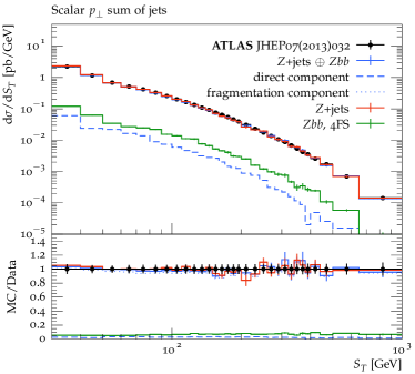
(b) The scalar sum of the transverse jet momenta, $S_{T}=\sum_{i}p_{\perp,i}^{\text{jet}}$.

Figure 3: Comparison of the newly developed algorithm with the established MEPS@NLO method and data from ATLAS in a $Z+\text{jets}$ region of phase space. The fused prediction is shown in solid blue, its both components are given as dashed and dotted blue lines. The 5FS MEPS@NLO and the 4FS MC@NLO are shown for comparison in red and green.

If the event selection does not explicitly require any $b$-jet, our fusing approach is expected to agree with the MEPS@NLO prediction. This is validated here with 7 TeV data from ATLAS Aad et al. (2013). In this measurement, $Z$ bosons decaying to electrons or muons were measured in association with jets. Leptons are required to have a transverse momentum of $p_{\perp}^{\ell}>20~{}\text{G$\text{e}\mspace{-0.8mu}\text{V}$}$ and a combined invariant mass with $66~{}\text{G$\text{e}\mspace{-0.8mu}\text{V}$}<m_{\ell\ell}<116~{}\text{G$\text{e}\mspace{-0.8mu}\text{V}$}$. Jets are defined by the anti-$k_{t}$ algorithm with $R=0.4$ with a transverse momentum of $p_{\perp}^{j}>30~{}\text{G$\text{e}\mspace{-0.8mu}\text{V}$}$ and a minimal angular distance to the leptons, $\Delta R(j,\ell)>0.5$.

In Fig. 3, the transverse momentum spectrum $p_{\perp}^{Z}$ of the $Z$ boson and the scalar sum of the jet transverse momenta, $S_{T}$, are shown. As expected, the fusing prediction is dominated by the fragmentation component in this region of phase space. The full 4FS prediction still reaches up to 10 % of the cross section, showing the necessity for a rigorous combination. In both distributions, the new prediction is compatible with the experimental data, and the agreement with the MEPS@NLO prediction demonstrates that the fusing algorithm does not induce any unexpected features.

V.2 Results in $Zbb$ phase space

	Data [pb]	Fusing [pb]	$Zbb$, 4F [pb]	$Z+\text{jets}$ [pb]
$Z+\geq 1b$	$3.55\pm 0.24_{\text{comb}}$	$3.80\pm 0.05_{\text{stat}}\pm\begin{array}[]{l}0.83\\ 0.33\end{array}\tiny{\text{pert}}$	$3.14\pm 0.03_{\text{stat}}$	$4.77\pm 0.10_{\text{stat}}$
$Z+\geq 2b$	$0.331\pm 0.037_{\text{comb}}$	$0.282\pm 0.004_{\text{stat}}\pm\begin{array}[]{l}0.027\\ 0.022\end{array}\tiny{\text{pert}}$	$0.305\pm 0.006_{\text{stat}}$	$0.358\pm 0.012_{\text{stat}}$

Table 1: The total cross section for having at least one or at least two $b$-jets. Different predictions are compared to data from CMS. The uncertainties given for the data are combined uncertainties, the predictions are given with their statistical (all) and perturbative (only fusing) uncertainties.

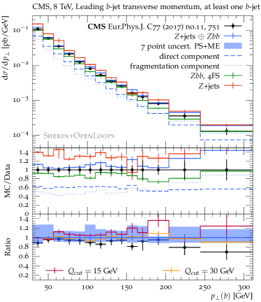
(a) The transverse momentum of the leading $b$-jet.

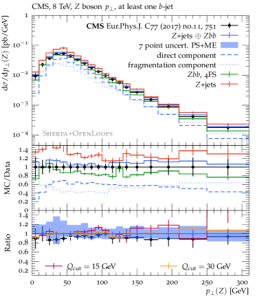
(b) The transverse momentum of the $Z$ boson.

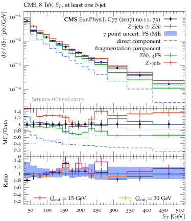
(c) The scalar sum of all transverse jet momenta, $S_{T}=\sum_{i}p_{\perp,i}^{\text{jet}}$.

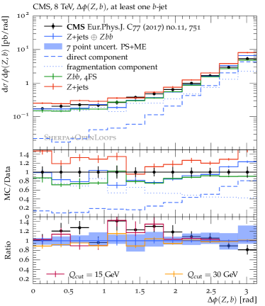
(d) The azimuthal distance between the leading $b$-jet and the $Z$-boson.

Figure 4: Comparison of the newly developed algorithm with data from CMS in a phase space region with at least one $b$-jet. The new fusing prediction is shown in solid blue, its both components are given as dashed and dotted blue lines. The 5FS MEPS@NLO and the 4FS MC@NLO are shown for comparison in red and green. The uncertainties for the fused prediction are shown in the second ratio plot. They include a simultaneous seven-point variation of $\mu_{\text{F}}$ and $\mu_{\text{R}}$ for both, matrix element and parton shower emissions, and a merging cut variation for $Q_{\text{cut}}=15(30)~{}\text{G$\text{e}\mspace{-0.8mu}\text{V}$}$.

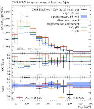
(a) The invariant mass distribution of the both leading $b$-jets.

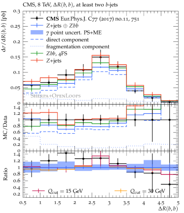
(b) The angular distance of the both leading $b$-jets.

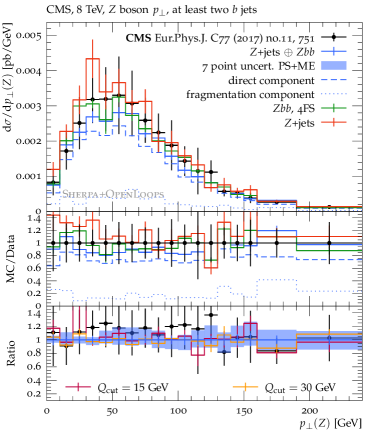
(c) The transverse momentum of the $Z$ boson.

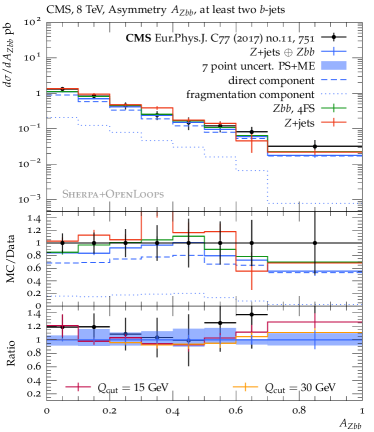
(d) The asymmetry $A_{Zbb}$, defined as $A_{Zbb}=\frac{\mathrm{\Delta}R^{\text{max}}(Z,b)-\mathrm{\Delta}R^{\text{min}}(Z,b)}{\mathrm{\Delta}R^{\text{max}}(Z,b)+\mathrm{\Delta}R^{\text{min}}(Z,b)}$.

Figure 5: Comparison of the newly developed algorithm with data from CMS in a phase space region with at least two $b$-jets. The new fusing prediction is shown in solid blue, its both components are given as dashed and dotted blue lines. The 5FS MEPS@NLO and the 4FS MC@NLO are shown for comparison in red and green. The uncertainties for the fused prediction are shown in the second ratio plot. They include a simultaneous seven-point variation of $\mu_{\text{F}}$ and $\mu_{\text{R}}$ for both, matrix element and parton shower emissions, and a merging cut variation for $Q_{\text{cut}}=15(30)~{}\text{G$\text{e}\mspace{-0.8mu}\text{V}$}$.

For the validation of our newly developed approach in a $Zbb$ region we use 8 TeV data taken by CMS Khachatryan et al. (2017). There, the $Z$ boson is reconstructed from either two electrons or two muons in a mass window between $71~{}\text{G$\text{e}\mspace{-0.8mu}\text{V}$}$ and $111~{}\text{G$\text{e}\mspace{-0.8mu}\text{V}$}$. These leptons are required to have $p_{\perp}>20~{}\text{G$\text{e}\mspace{-0.8mu}\text{V}$}$ and $|\eta|<2.4$, and are dressed with photons within a cone of $\Delta R<0.1$. Jets are defined by the anti-$k_{t}$ algorithm with $R=0.5$, $p_{\perp}>30~{}\text{G$\text{e}\mspace{-0.8mu}\text{V}$}$ and $|\eta|<2.4$. Only jets with no overlap ($\Delta R>0.5$) to leptons are taken into account. $b$-jets are identified by ghost association Cacciari and Salam (2008) and have to pass the same jet cuts as described above.

Again, we compare our newly obtained prediction to the experimental data and to predictions obtained in the 4FS and 5FS. In addition, we estimate the perturbative uncertainties and the uncertainties related to the merging scale. The former are given by 7-point variations of $\mu_{\text{R}}$ and $\mu_{\text{F}}$ coherently in the matrix elements and the parton shower. The latter are studied by a variation of the merging cut to values of $15$ or $30~{}\text{G$\text{e}\mspace{-0.8mu}\text{V}$}$. The total cross sections for having at least one or at least two $b$-jets are displayed in Table 1 and differential distributions for one (two) $b$-jet observables are shown in Fig. 4 (Fig. 5).

In the one $b$-jet region, the predicted cross sections of the fused result and the 4FS prediction are in good agreement with the data, whereas the 5FS prediction exceeds it by 34 %. Differential cross sections for several distributions are given in Fig. 4. In general, the fused prediction is in good agreement with the data and in between the 4FS and 5FS predictions. Whereas the former slightly undershoots the data, the latter has a significantly larger cross section. This holds in particular for small transverse momenta of either the $b$-jet or the $Z$ boson or if the $b$-jet is close to the $Z$ boson. Both fusing components are equally relevant in all distributions, with a highly non-trivial phase-space dependence of their relative contributions. While they are relatively flat and equal in the transverse-momentum spectrum of the leading $b$-jet, the direct component dominates around the peak of $p_{\perp}(Z)$. A different composition is found in the $S_{T}$ distribution and for $\mathrm{\Delta}\Phi(Z,b)$. At large $S_{T}$ or small $\mathrm{\Delta}\Phi(Z,b)$ the fragmentation contribution takes over and the direct one only contributes with around 20 %. At the same time, the 4FS prediction undershoots the high $S_{T}$ region. This region is sensitive to a good modeling of multiple hard jets, which can only be predicted reliably by multi-jet matrix elements. This is the case in the fusing procedure, where in the fragmentation component the hard emissions are generated first by matrix elements and $b$ quarks may be produced later on in the shower. In the 4FS prediction on the other hand, the $b$-quarks are always described by matrix elements and additional emissions of light partons by the parton shower can form hard jets in the end. Thus, the modeling of this region with a 4FS prediction becomes very sensitive to the parton shower which is applied outside its region of validity. The uncertainties related to the merging scale in the fragmentation component and the perturbative uncertainties are depicted in the lower ratio-plots in Fig. 4 for all distributions. The perturbative uncertainties are at the level of 15-20 % in all observables. Results with different merging cuts are all within the perturbative uncertainty band and in good agreement with each other. The $Q_{\text{cut}}=15~{}\text{G$\text{e}\mspace{-0.8mu}\text{V}$}$ curve has significantly higher statistical uncertainties, which is a typical feature for multi-jet merged predictions with very low merging scales.

In the two-$b$-jet region, the total predicted cross sections of both the 4FS and 5FS are in good agreement with the experimentally measured ones. The fused prediction is slightly lower but still matches the data within the uncertainties. Differential distributions for this region of phase space are given in Fig. 5. Here, both the 4FS and the 5FS curve are in good agreement with each other and with the experimental data. The fused prediction follows very closely the 4FS result but has a slightly smaller cross section in some bins. In all regions of phase space, the direct component gives the dominant contribution of the fused prediction. Only for $b$-jet pairs which are collimated or have a small invariant mass, the fragmentation component exceeds the 20 % threshold, which demonstrates the expected transition towards unresolved one-$b$-jet configurations. The perturbative uncertainties are reduced in comparison to the one-$b$-jet region. They are at the level of 5 % for low values of $p_{\perp}^{Z}$ and reach up to 15 % for larger values. Again, all merging cut variations are within the perturbative uncertainty band, with the $Q_{\text{cut}}=15~{}\text{G$\text{e}\mspace{-0.8mu}\text{V}$}$ curve again yielding large statistical uncertainties in some bins. It is worth noting that the fused prediction has a significantly smaller statistical uncertainty than the 5FS prediction, although the fragmentation component was generated with the same number of events. This is expected in all regions of phase space where the direct component dominates since only a small fraction of 5FS events will yield two $b$-jets. The direct component profits from its explicit production of heavy-flavor final states and can fill the phase space more efficiently.

VI Conclusions

We have presented a novel event generation algorithm to simulate heavy-flavor associated production in collider experiments. Building upon the established merging algorithms for multi-jet matrix elements and parton showers, we propose a technique to include massive matrix elements for heavy-quark production, effectively leading to an MC simulation in a variable-flavor-number scheme, which we call fusing.

The overlap between the five- and four-flavor scheme calculations is removed based on a parton-shower interpretation of the full parton evolution from the hard scale to the parton shower cut-off. This evolution history is also used to supplement the massive matrix elements with all higher-order corrections necessary to maintain the logarithmic accuracy of the multi-jet merged calculation.

Our algorithm allows to combine the advantages of inclusive five-flavor scheme calculations with the higher precision of four-flavor scheme calculations in regions of phase space where the bottom quark mass sets a relevant scale. Such a combined prediction is crucial for heavy-flavor measurements in LHC experiments, since they will always be affected by the presence of fake heavy-flavor tagged jets.

The fusing algorithm can be applied at leading order or next-to-leading order QCD. Its logarithmic accuracy depends on the parton shower used in the merging and might be extended to NLL in the near future. The relation to the FONLL method has been established by analytically identifying the known FONLL matching coefficients within the fused parton shower expressions.

Using an implementation in the Sherpa event generator, we show a first application to heavy-flavor production in association with a $Z$ boson. Cross checks of exclusive observables and a comparison of the results for heavy-flavor production to experimental data demonstrate the improvement over existing multi-jet merging algorithms.

Appendix A Correspondence between inclusive and exclusive parton evolution

In this appendix we summarize the correspondence between the exclusive parton evolution implemented by parton showers and the underlying inclusive evolution equations. In the collinear limit, the evolution of parton densities $f_{a}(x,t)$ is determined by the DGLAP equations Gribov and Lipatov (1972); Lipatov (1975); Dokshitzer (1977); Altarelli and Parisi (1977)

$$\frac{{\rm d}\,xf_{a}(x,t)}{{\rm d}\ln t}=\sum_{b=q,g}\int_{0}^{1}{\rm d}\tau\int_{0}^{1}{\rm d}z\,\frac{\alpha_{s}}{2\pi}\big{[}z\hat{P}_{ba}(z)\big{]}_{+}\,\tau f_{b}(\tau,t)\,\delta(x-\tau z)\;.$$ (25)

In this context, $\hat{P}_{ba}$ are the unregularized DGLAP evolution kernels, which can be expanded into a power series in the strong coupling. The plus prescription is employed to enforce the momentum and flavor sum rules as

$$zP_{ba}(z)=\big{[}z\hat{P}_{ba}(z)\big{]}_{+}=\lim\limits_{\varepsilon\to 0}z\hat{P}_{ba}(z,\varepsilon)\;,$$ (26)

where

$$\hat{P}_{ba}(z,\varepsilon)=\hat{P}_{ba}(z)\,\Theta(1-z-\varepsilon)-\delta_{ab}\sum_{c\in\{q,g\}}\frac{\Theta(z-1+\varepsilon)}{\varepsilon}\int_{0}^{1-\varepsilon}{\rm d}\zeta\,\zeta\,\hat{P}_{ac}(\zeta)\;.$$ (27)

For finite $\varepsilon$, the endpoint subtraction in Eq. (26) can be interpreted as the approximate virtual plus unresolved real corrections, which are included in the parton shower because the Monte-Carlo algorithm implements a unitarity constraint Jadach and Skrzypek (2004). The precise value of $\varepsilon$ is determined in terms of an infrared cutoff on the evolution variable, by means of four-momentum conservation Höche et al. (2018). For $0<\varepsilon\ll 1$, Eq. (25) can be written as

$$\frac{1}{f_{a}(x,t)}\,\frac{{\rm d}f_{a}(x,t)}{{\rm d}\ln t}=-\sum_{c=q,g}\int_{0}^{1-\varepsilon}{\rm d}\zeta\,\zeta\,\frac{\alpha_{s}}{2\pi}\hat{P}_{ac}(\zeta)\,+\sum_{b=q,g}\int_{x}^{1-\varepsilon}\frac{{\rm d}z}{z}\,\frac{\alpha_{s}}{2\pi}\,\hat{P}_{ba}(z)\,\frac{f_{b}(x/z,t)}{f_{a}(x,t)}\;.$$ (28)

Using the Sudakov factor of the parton shower

$$\Delta_{a}(t_{0},t)=\exp\bigg{\{}-\int_{t_{0}}^{t}\frac{{\rm d}\bar{t}}{\bar{t}}\sum_{c=q,g}\int_{0}^{1-\varepsilon}{\rm d}\zeta\,\zeta\,\frac{\alpha_{s}}{2\pi}\hat{P}_{ac}(\zeta)\bigg{\}}$$ (29)

one can define the generating function for splittings of parton $a$ as

$$\mathcal{F}_{a}(x,t,\mu^{2})=f_{a}(x,t)\Delta_{a}(t,\mu^{2})\;.$$ (30)

Equation (28) can then be reduced to

$$\frac{{\rm d}\ln\mathcal{F}_{a}(x,t,\mu^{2})}{{\rm d}\ln t}=\sum_{b=q,g}\int_{x}^{1-\varepsilon}\frac{{\rm d}z}{z}\,\frac{\alpha_{s}}{2\pi}\,\hat{P}_{ba}(z)\,\frac{f_{b}(x/z,t)}{f_{a}(x,t)}\;.$$ (31)

It is solved using the Markovian Monte-Carlo techniques implemented by parton showers. Note that Eq. (31) is structurally equivalent to the inclusive result, Eq. (25), which can be written as

$$\frac{{\rm d}\ln f_{a}(x,t)}{{\rm d}\ln t}=\sum_{b=q,g}\int_{x}^{1}\frac{{\rm d}z}{z}\,\frac{\alpha_{s}}{2\pi}\,P_{ba}(z)\,\frac{f_{b}(x/z,t)}{f_{a}(x,t)}\;.$$ (32)

In the context of our analysis in Sec. IV.2 it is important to remember this formal correspondence, which can be rephrased as the equivalence of the regularized DGLAP splitting kernels, $P_{ab}(z)$, and the splitting kernels $P_{ab}(z,\varepsilon)$ defined in Eq. (27) as $\varepsilon\to 0$. While this limit cannot be taken in the parton shower in practice Höche et al. (2018), it is a useful theoretical construction to prove that the Monte-Carlo algorithm and the inclusive parton evolution generate formally identical results to any logarithmic accuracy that is implemented by both calculations.

Appendix B Leading and next-to-leading order coefficient functions

The leading-order DGLAP splitting functions used in Sec. IV are defined as Gribov and Lipatov (1972); Dokshitzer (1977); Altarelli and Parisi (1977)

$$\begin{split}P_{qq}(z)=&\;C_{F}\,\frac{1+z^{2}}{(1-z)_{+}}+\frac{3}{2}\,C_{F}\,\delta(1-z)\;,&P_{qg}(z)=&\;C_{F}\,\frac{1+(1-z)^{2}}{z}\;,\\ P_{gq}(z)=&\;T_{R}\left(1-2z(1-z)\right)\;,&P_{gg}(z)=&\;2C_{A}\left(\frac{z}{(1-z)_{+}}+\frac{1-z}{z}+z(1-z)\right)+\beta_{0}\,\delta(1-z)\;.\end{split}$$ (33)

The next-to-leading order splitting functions needed to evaluate Eq. (8) are given by Curci et al. (1980); Furmanski and Petronzio (1980); Floratos et al. (1981a, b); Heinrich and Kunszt (1998); Ellis and Vogelsang (1996)

$$\begin{split}&P_{qq}^{S,(1)}(z)=C_{F}T_{R}\left[-(1+z)\ln^{2}z+\left(\frac{8}{3}z^{2}+5z+1\right)\ln z-\frac{56}{9}z^{2}+6z-2+\frac{20}{9z}\,\right]\;,\\ &P_{gq}^{(1)}(z)=C_{F}T_{R}\bigg{[}\,2-\frac{9}{2}z-\left(\frac{1}{2}-2z\right)\ln z-\left(\frac{1}{2}-z\right)\ln^{2}z+2\ln(1-z)\\ &\qquad\qquad\qquad\qquad+\bigg{(}\ln^{2}\frac{1-z}{z}-2\ln\frac{1-z}{z}-\frac{\pi^{2}}{3}+5\bigg{)}\frac{P_{gq}(z)}{T_{R}}\bigg{]}\\ &\qquad+C_{A}T_{R}\bigg{[}\frac{91}{9}+\frac{7}{9}z+\frac{20}{9z}+\left(\frac{68}{3}z-\frac{19}{3}\right)\ln z-2\ln(1-z)-(1+4z)\ln^{2}z+S_{2}(z)\frac{P_{gq}(-z)}{T_{R}}\\ &\qquad\qquad\qquad\quad+\left(-\frac{1}{2}\ln^{2}z+\frac{22}{3}\ln z-\ln^{2}(1-z)+2\ln(1-z)+\frac{\pi^{2}}{6}-\frac{109}{9}\right)\frac{P_{gq}(z)}{T_{R}}\,\bigg{]}\;.\\ &P_{qq,Q}^{V,(1)}(z)=C_{F}T_{R}\left[-\left(\frac{2}{3}\ln z+\frac{10}{9}\right)\frac{1+z^{2}}{1-z}-\frac{4}{3}(1-z)\,\right]_{+}\;,\\ \end{split}$$ (34)

The auxiliary function $S_{2}$ is defined as Ellis et al. (1996)

$$\begin{split}S_{2}(z)=\;&-2\,{\rm Li}_{2}\Big{(}\frac{1}{1+z}\Big{)}+\frac{1}{2}\log^{2}z-\log^{2}(1-z)+\frac{\pi^{2}}{6}\;.\end{split}$$ (35)

The $\beta$ function coefficients used in Sec. IV are

$$\begin{split}\beta_{0}=&\frac{11}{6}C_{A}-\frac{2}{3}T_{R}n_{f}\;,&\beta_{0,b}&=-\frac{2}{3}T_{R}\;.\end{split}$$ (36)

Note that $n_{f}$ counts the number of light parton flavors only Buza et al. (1996).

References

- Aaboud et al. (2018a) M. Aaboud et al. (ATLAS), Phys. Lett. B786, 59 (2018a), eprint 1808.08238.
- Sirunyan et al. (2018a) A. M. Sirunyan et al. (CMS), Phys. Rev. Lett. 121, 121801 (2018a), eprint 1808.08242.
- Sirunyan et al. (2018b) A. M. Sirunyan et al. (CMS), Phys. Rev. Lett. 120, 231801 (2018b), eprint 1804.02610.
- Aaboud et al. (2018b) M. Aaboud et al. (ATLAS), Phys. Rev. D97, 072016 (2018b), eprint 1712.08895.
- de Florian et al. (2016) D. de Florian et al. (LHC Higgs Cross Section Working Group) (2016), eprint 1610.07922.
- Alekhin et al. (2010) S. Alekhin, J. Blumlein, S. Klein, and S. Moch, Phys. Rev. D81, 014032 (2010), eprint 0908.2766.
- Aivazis et al. (1994a) M. A. G. Aivazis, F. I. Olness, and W.-K. Tung, Phys. Rev. D50, 3085 (1994a), eprint hep-ph/9312318.
- Aivazis et al. (1994b) M. A. G. Aivazis, J. C. Collins, F. I. Olness, and W.-K. Tung, Phys. Rev. D50, 3102 (1994b), eprint hep-ph/9312319.
- Tung et al. (2002) W.-K. Tung, S. Kretzer, and C. Schmidt, J. Phys. G28, 983 (2002), eprint hep-ph/0110247.
- Kniehl et al. (2011) B. A. Kniehl, G. Kramer, I. Schienbein, and H. Spiesberger, Phys. Rev. D84, 094026 (2011), eprint 1109.2472.
- Thorne and Roberts (1998) R. S. Thorne and R. G. Roberts, Phys. Rev. D57, 6871 (1998), eprint hep-ph/9709442.
- Thorne (2006) R. S. Thorne, Phys. Rev. D73, 054019 (2006), eprint hep-ph/0601245.
- Cacciari et al. (1998) M. Cacciari, M. Greco, and P. Nason, JHEP 05, 007 (1998), eprint hep-ph/9803400.
- Forte et al. (2010) S. Forte, E. Laenen, P. Nason, and J. Rojo, Nucl. Phys. B834, 116 (2010), eprint 1001.2312.
- Kusina et al. (2013) A. Kusina, F. I. Olness, I. Schienbein, T. Jezo, K. Kovarik, T. Stavreva, and J. Y. Yu, Phys. Rev. D88, 074032 (2013), eprint 1306.6553.
- Krauss and Napoletano (2018) F. Krauss and D. Napoletano, Phys. Rev. D98, 096002 (2018), eprint 1712.06832.
- Dittmaier et al. (2004) S. Dittmaier, M. Krämer, and M. Spira, Phys. Rev. D70, 074010 (2004), eprint hep-ph/0309204.
- Dawson et al. (2004) S. Dawson, C. B. Jackson, L. Reina, and D. Wackeroth, Phys. Rev. D69, 074027 (2004), eprint hep-ph/0311067.
- Febres Cordero et al. (2008) F. Febres Cordero, L. Reina, and D. Wackeroth, Phys. Rev. D78, 074014 (2008), eprint 0806.0808.
- Febres Cordero et al. (2009) F. Febres Cordero, L. Reina, and D. Wackeroth, Phys. Rev. D80, 034015 (2009), eprint 0906.1923.
- Campbell et al. (2012) J. M. Campbell, F. Caola, F. Febres Cordero, L. Reina, and D. Wackeroth, Phys. Rev. D86, 034021 (2012), eprint 1107.3714.
- Campbell et al. (2009) J. M. Campbell, R. K. Ellis, F. Febres Cordero, F. Maltoni, L. Reina, D. Wackeroth, and S. Willenbrock, Phys. Rev. D79, 034023 (2009), eprint 0809.3003.
- Forte et al. (2015) S. Forte, D. Napoletano, and M. Ubiali, Phys. Lett. B751, 331 (2015), eprint 1508.01529.
- Forte et al. (2016) S. Forte, D. Napoletano, and M. Ubiali, Phys. Lett. B763, 190 (2016), eprint 1607.00389.
- Forte et al. (2018) S. Forte, D. Napoletano, and M. Ubiali, Eur. Phys. J. C78, 932 (2018), eprint 1803.10248.
- Bonvini et al. (2015) M. Bonvini, A. S. Papanastasiou, and F. J. Tackmann, JHEP 11, 196 (2015), eprint 1508.03288.
- Bonvini et al. (2016) M. Bonvini, A. S. Papanastasiou, and F. J. Tackmann, JHEP 10, 053 (2016), eprint 1605.01733.
- Febres Cordero and Reina (2015) F. Febres Cordero and L. Reina, Int. J. Mod. Phys. A30, 1530042 (2015), eprint 1504.07177.
- Figueroa et al. (2018) D. Figueroa, S. Honeywell, S. Quackenbush, L. Reina, C. Reuschle, and D. Wackeroth, Phys. Rev. D98, 093002 (2018), eprint 1805.01353.
- Buckley et al. (2011) A. Buckley et al., Phys. Rept. 504, 145 (2011), eprint 1101.2599.
- Bellm et al. (2016) J. Bellm et al., Eur. Phys. J. C76, 196 (2016), eprint 1512.01178.
- Sjöstrand et al. (2014) T. Sjöstrand, S. Ask, J. R. Christiansen, R. Corke, N. Desai, P. Ilten, S. Mrenna, S. Prestel, C. O. Rasmussen, and P. Z. Skands (2014), eprint 1410.3012.
- Gleisberg et al. (2009) T. Gleisberg, S. Höche, F. Krauss, M. Schönherr, S. Schumann, F. Siegert, and J. Winter, JHEP 02, 007 (2009), eprint 0811.4622.
- Norrbin and Sjöstrand (2001) E. Norrbin and T. Sjöstrand, Nucl. Phys. B603, 297 (2001), eprint hep-ph/0010012.
- Schumann and Krauss (2008) S. Schumann and F. Krauss, JHEP 03, 038 (2008), eprint 0709.1027.
- Höche and Prestel (2015) S. Höche and S. Prestel, Eur. Phys. J. C75, 461 (2015), eprint 1506.05057.
- Cabouat and Sjöstrand (2018) B. Cabouat and T. Sjöstrand, Eur. Phys. J. C78, 226 (2018), eprint 1710.00391.
- Cormier et al. (2018) K. Cormier, S. Plätzer, C. Reuschle, P. Richardson, and S. Webster (2018), eprint 1810.06493.
- Frixione and Webber (2002) S. Frixione and B. R. Webber, JHEP 06, 029 (2002), eprint hep-ph/0204244.
- Nason (2004) P. Nason, JHEP 11, 040 (2004), eprint hep-ph/0409146.
- Frixione et al. (2007) S. Frixione, P. Nason, and C. Oleari, JHEP 11, 070 (2007), eprint 0709.2092.
- Höche et al. (2012) S. Höche, F. Krauss, M. Schönherr, and F. Siegert, JHEP 09, 049 (2012), eprint 1111.1220.
- Plätzer and Gieseke (2012) S. Plätzer and S. Gieseke, Eur.Phys.J. C72, 2187 (2012), eprint 1109.6256.
- Frederix et al. (2011) R. Frederix, S. Frixione, V. Hirschi, F. Maltoni, R. Pittau, and P. Torrielli, JHEP 09, 061 (2011), eprint 1106.6019.
- Oleari and Reina (2011) C. Oleari and L. Reina, JHEP 08, 061 (2011), eprint 1105.4488.
- Bagnaschi et al. (2018) E. Bagnaschi, F. Maltoni, A. Vicini, and M. Zaro, JHEP 07, 101 (2018), eprint 1803.04336.
- Krauss et al. (2017) F. Krauss, D. Napoletano, and S. Schumann, Phys. Rev. D95, 036012 (2017), eprint 1612.04640.
- Cascioli et al. (2013) F. Cascioli, P. Maierhoefer, N. Moretti, S. Pozzorini, and F. Siegert (2013), eprint 1309.5912.
- Ježo et al. (2018) T. Ježo, J. M. Lindert, N. Moretti, and S. Pozzorini, Eur. Phys. J. C78, 502 (2018), eprint 1802.00426.
- Bevilacqua et al. (2017) G. Bevilacqua, M. V. Garzelli, and A. Kardos (2017), eprint 1709.06915.
- Catani et al. (2001) S. Catani, F. Krauss, R. Kuhn, and B. R. Webber, JHEP 11, 063 (2001), eprint hep-ph/0109231.
- Mangano et al. (2002) M. L. Mangano, M. Moretti, and R. Pittau, Nucl. Phys. B632, 343 (2002), eprint hep-ph/0108069.
- Krauss (2002) F. Krauss, JHEP 08, 015 (2002), eprint hep-ph/0205283.
- Lönnblad (2002) L. Lönnblad, JHEP 05, 046 (2002), eprint hep-ph/0112284.
- Lavesson and Lönnblad (2008) N. Lavesson and L. Lönnblad, JHEP 04, 085 (2008), eprint 0712.2966.
- Alwall et al. (2008) J. Alwall et al., Eur. Phys. J. C53, 473 (2008), eprint 0706.2569.
- Höche et al. (2009) S. Höche, F. Krauss, S. Schumann, and F. Siegert, JHEP 05, 053 (2009), eprint 0903.1219.
- Hamilton et al. (2009) K. Hamilton, P. Richardson, and J. Tully, JHEP 11, 038 (2009), eprint 0905.3072.
- Lönnblad and Prestel (2012) L. Lönnblad and S. Prestel, JHEP 03, 019 (2012), eprint 1109.4829.
- Höche et al. (2013) S. Höche, F. Krauss, M. Schönherr, and F. Siegert, JHEP 04, 027 (2013), eprint 1207.5030.
- Gehrmann et al. (2013) T. Gehrmann, S. Höche, F. Krauss, M. Schönherr, and F. Siegert, JHEP 01, 144 (2013), eprint 1207.5031.
- Lönnblad and Prestel (2013) L. Lönnblad and S. Prestel, JHEP 03, 166 (2013), eprint 1211.7278.
- Frederix and Frixione (2012) R. Frederix and S. Frixione, JHEP 12, 061 (2012), eprint 1209.6215.
- Bellm et al. (2018) J. Bellm, S. Gieseke, and S. Plätzer, Eur. Phys. J. C78, 244 (2018), eprint 1705.06700.
- André and Sjöstrand (1998) J. André and T. Sjöstrand, Phys. Rev. D57, 5767 (1998), eprint hep-ph/9708390.
- Amati et al. (1980) D. Amati, A. Bassetto, M. Ciafaloni, G. Marchesini, and G. Veneziano, Nucl. Phys. B173, 429 (1980).
- Catani et al. (1991) S. Catani, B. R. Webber, and G. Marchesini, Nucl. Phys. B349, 635 (1991).
- Bauer et al. (2017) C. W. Bauer, N. Ferland, and B. R. Webber, JHEP 08, 036 (2017), eprint 1703.08562.
- Bauer and Webber (2019) C. W. Bauer and B. R. Webber, JHEP 03, 013 (2019), eprint 1808.08831.
- Fornal et al. (2018) B. Fornal, A. V. Manohar, and W. J. Waalewijn, JHEP 05, 106 (2018), eprint 1803.06347.
- Buza et al. (1998) M. Buza, Y. Matiounine, J. Smith, and W. L. van Neerven, Eur. Phys. J. C1, 301 (1998), eprint hep-ph/9612398.
- Buza et al. (1996) M. Buza, Y. Matiounine, J. Smith, R. Migneron, and W. L. van Neerven, Nucl. Phys. B472, 611 (1996), eprint hep-ph/9601302.
- Höche and Prestel (2017) S. Höche and S. Prestel, Phys. Rev. D96, 074017 (2017), eprint 1705.00742.
- Dulat et al. (2018) F. Dulat, S. Höche, and S. Prestel, Phys. Rev. D98, 074013 (2018), eprint 1805.03757.
- Krauss et al. (2002) F. Krauss, R. Kuhn, and G. Soff, JHEP 02, 044 (2002), eprint hep-ph/0109036.
- Gleisberg and Höche (2008) T. Gleisberg and S. Höche, JHEP 12, 039 (2008), eprint 0808.3674.
- Cascioli et al. (2012) F. Cascioli, P. Maierhöfer, and S. Pozzorini, Phys.Rev.Lett. 108, 111601 (2012), eprint 1111.5206.
- Ossola et al. (2008) G. Ossola, C. G. Papadopoulos, and R. Pittau, JHEP 0803, 042 (2008), eprint 0711.3596.
- van Hameren (2011) A. van Hameren, Comput.Phys.Commun. 182, 2427 (2011), eprint 1007.4716.
- Ball et al. (2015) R. D. Ball et al. (NNPDF), JHEP 04, 040 (2015), eprint 1410.8849.
- Buckley et al. (2015) A. Buckley, J. Ferrando, S. Lloyd, K. Nordström, B. Page, M. Rüfenacht, M. Schönherr, and G. Watt, Eur. Phys. J. C75, 132 (2015), eprint 1412.7420.
- Hoeche et al. (2014) S. Hoeche, F. Krauss, and M. Schonherr (2014), eprint 1401.7971.
- Sjöstrand and van Zijl (1987) T. Sjöstrand and M. van Zijl, Phys. Rev. D36, 2019 (1987).
- De Roeck and Jung (2005) A. De Roeck and H. Jung, eds., HERA and the LHC: A Workshop on the implications of HERA for LHC physics: Proceedings Part A, CERN (CERN, Geneva, 2005), eprint hep-ph/0601012.
- Winter et al. (2004) J.-C. Winter, F. Krauss, and G. Soff, Eur. Phys. J. C36, 381 (2004), eprint hep-ph/0311085.
- Buckley et al. (2013) A. Buckley, J. Butterworth, L. Lönnblad, D. Grellscheid, H. Hoeth, et al., Comput.Phys.Commun. 184, 2803 (2013), eprint 1003.0694.
- Bothmann et al. (2016) E. Bothmann, M. Schönherr, and S. Schumann, Eur. Phys. J. C76, 590 (2016), eprint 1606.08753.
- Aad et al. (2013) G. Aad et al. (ATLAS), JHEP 07, 032 (2013), eprint 1304.7098.
- Khachatryan et al. (2017) V. Khachatryan et al. (CMS), Eur. Phys. J. C77, 751 (2017), eprint 1611.06507.
- Cacciari and Salam (2008) M. Cacciari and G. P. Salam, Phys. Lett. B659, 119 (2008), eprint 0707.1378.
- Gribov and Lipatov (1972) V. N. Gribov and L. N. Lipatov, Sov. J. Nucl. Phys. 15, 438 (1972).
- Lipatov (1975) L. N. Lipatov, Sov. J. Nucl. Phys. 20, 94 (1975).
- Dokshitzer (1977) Y. L. Dokshitzer, Sov. Phys. JETP 46, 641 (1977).
- Altarelli and Parisi (1977) G. Altarelli and G. Parisi, Nucl. Phys. B126, 298 (1977).
- Jadach and Skrzypek (2004) S. Jadach and M. Skrzypek, Acta Phys. Polon. B35, 745 (2004), eprint hep-ph/0312355.
- Höche et al. (2018) S. Höche, D. Reichelt, and F. Siegert, JHEP 01, 118 (2018), eprint 1711.03497.
- Curci et al. (1980) G. Curci, W. Furmanski, and R. Petronzio, Nucl. Phys. B175, 27 (1980).
- Furmanski and Petronzio (1980) W. Furmanski and R. Petronzio, Phys. Lett. B97, 437 (1980).
- Floratos et al. (1981a) E. G. Floratos, R. Lacaze, and C. Kounnas, Phys. Lett. B98, 89 (1981a).
- Floratos et al. (1981b) E. G. Floratos, R. Lacaze, and C. Kounnas, Phys. Lett. B98, 285 (1981b).
- Heinrich and Kunszt (1998) G. Heinrich and Z. Kunszt, Nucl. Phys. B519, 405 (1998), eprint hep-ph/9708334.
- Ellis and Vogelsang (1996) R. K. Ellis and W. Vogelsang (1996), eprint hep-ph/9602356.
- Ellis et al. (1996) R. K. Ellis, W. J. Stirling, and B. R. Webber, QCD and collider physics, vol. 8 (Cambridge Monogr. Part. Phys. Nucl. Phys. Cosmol., 1996), 1st ed.