Hints of Modified Gravity in Cosmos and in the Lab?

Abstract

General Relativity (GR) is consistent with a wide range of experiments/observations from millimeter scales up to galactic scales and beyond. However, there are reasons to believe that GR may need to be modified because it includes singularities (it is an incomplete theory) and also it requires fine-tuning to explain the accelerating expansion of the universe through the cosmological constant. Therefore, it is important to check various experiments and observations beyond the above range of scales for possible hints of deviations from the predictions of GR. If such hints are found it is important to understand which classes of modified gravity theories are consistent with them. The goal of this review is to summarize recent progress on these issues. On sub millimeter scales we show an analysis of the data of the Washington experiment Kapner et al. (2007a) searching for modifications of Newton’s Law on sub-millimeter scales and demonstrate that a spatially oscillating signal is hidden in this dataset. We demonstrate that even though this signal cannot be explained in the context of standard modified theories (viable scalar tensor and $f(R)$ theories), it is a rather generic prediction of nonlocal gravity theories. On cosmological scales we review recent analyses of Redshift Space Distortion (RSD) data which measure the growth rate of cosmological perturbations at various redshifts and show that these data are in some tension with the $\Lambda$CDM parameter values indicated by Planck/2015 CMB data at about 3$\sigma$ level. This tension can be reduced by allowing for an evolution of the effective Newton constant that determines the growth rate of cosmological perturbations. We conclude that even though this tension between the data and the predictions of GR could be due to systematic/statistical uncertainties of the data, it could also constitute early hints pointing towards a new gravitational theory.

I Introduction

General Relativity (GR) has been tested in a wide range of scales starting from sub-mm scales out to supercluster $O(100Mpc)$ scales. Even though no statistically significant evidence has been found so far indicating deviations from GR, there are theoretical arguments and experimental/observational hints that indicate that GR may need to be modified on both the smallest and the largest probed scales.

From the theoretical point of view, it is clear that GR has to face the following challenges:

• It predicts the existence of unphysical singularities which indicate that it is a physically incomplete theory.

• It is nonrenormalizable and inconsistent with Quantum Field Theory (QFT) at high energies due to the prediction of black hole formation when small scales are probed via scattering experiments.

• It can not explain the observed accelerating expansion of the universe unless extreme fine tuning is assumed.

From the experimental/observational point of view GR has been well tested on solar system scales where the PPN parameters measuring deviations from GR have been shown to reduce to the values predicted by GR at an accuracy level of about $10^{-5}$ Will (2014). On larger and smaller scales however the constraints on deviations from GR are not as strong. In fact there have been claims for hints of deviations from GR predictions even on solar system scales (e.g. Pioneer anomaly Anderson et al. (2002)) and on galactic scales (e.g. the formation of black holes at discrete values of mass Sokolov (2016)).

On galactic scales, the deviation of star velocities from the velocities expected in the presence of visible matter in the context of GR indicates that the Einstein equation $G_{\mu\nu}=T_{\mu\nu}^{lum}$ (where $T_{\mu\nu}^{lum}$ is the energy momentum tensor of luminous matter) is violated. The usual approach is restoring consistency between the two sides of the Einstein equation has been to modify the right side of the Einstein equation and write it in the form $G_{\mu\nu}=T_{\mu\nu}^{lum}+T_{\mu\nu}^{dm}$ where $T_{\mu\nu}^{dm}$ is the energy momentum tensor of matter that interacts only gravitationally (dark matter Jungman et al. (1996)). An alternative approach is to modify the left side of the Einstein equation as $G_{\mu\nu}+G_{\mu\nu}^{TeVeS}=T_{\mu\nu}^{lum}$ leading to a modified version of GR: Tensor Vector Scalar theory (TeVeS) Bekenstein (2004). Clearly, a combination of the above solutions is also possible leading to $G_{\mu\nu}+G_{\mu\nu}^{TeVeS}=T_{\mu\nu}^{lum}+T_{\mu\nu}^{dm}$. The recent detection of gravitational waves coming from the collision of two neutron stars (GW170817) Abbott et al. (2017a), however, seems to exclude Boran et al. (2018) all types of dark matter emulator theories such as TeVeS theory. An exception to this exclusion may be Green et al. (2018) the alternative Scalar-Tensor-Vector Gravity theory (STVG) Moffat (2006), which seems to remain viable after the GW170817 event since the photon and graviton geodesics are identical in this theory. Another modified dark matter emulator approach similar to the Modified Newtonian Dynamics (MOND) approach Milgrom (1983a, b, c) is based on the assumption that the gravitational constant varies with acceleration Christodoulou and Kazanas (2018, 2019a, 2019b) or equivalently with the dimensionless surface density of a spherical mass distribution $s$ Christodoulou and Kazanas (2019c).

The frontiers of current gravitational research lie on the two extreme scales that gravitational experiments/observations can currently probe: sub-mm scales where a wide range of experiments Murata and Tanaka (2015) search for new types of forces and cosmological scales of a few $Mpc$ or larger where observations of the growth rate of cosmological perturbations through Redsift Space Distortions Nesseris et al. (2017); Macaulay et al. (2013); Tsujikawa (2015); Johnson et al. (2016); Basilakos and Nesseris (2017); Kazantzidis and Perivolaropoulos (2018) or Weak Lensing Joudaki et al. (2018); Hildebrandt et al. (2017); Troxel et al. (2018); Köhlinger et al. (2017) can probe the gravitational laws and the consistency of GR with data. Current research on these frontier scales is the focus of the present review.

Small scale gravity experiments Lamoreaux (1997); Chiaverini et al. (2003); Smullin et al. (2005); Geraci et al. (2008); Long et al. (2002); Mitrofanov and Ponomareva (1988); Hoyle et al. (2004a, 2001); Kapner et al. (2007b); Tu et al. (2007); Yang et al. (2012); et. al. (2014); Hoskins et al. (1985); Spero et al. (1980); Milyukov (1985); Panov and Frontov (1979); Moody and Paik (1993); H. et al. (1980); Y. et al. (1982); K. and H. (1985); N. et al. (1987) probe sub-mm scales searching for new forces on these scales. The forces between test masses are measured at various distances and compared with the expected forces on the basis of known physics. Deviations from the null result corresponding to Newtonian gravitational interaction are fit to specific parametrizations that are well motivated based on theoretical arguments. The most commonly used parametrization for fitting the above deviations of gravitational experiment data is the Yukawa parametrization, where the effective gravitational interaction potential is expressed as

$$V_{\rm eff}=-G\frac{M}{r}(1+\alpha e^{-mr})$$ (1)

corresponding to a spatially varying effective Newton’s constant of the form

$$G_{\rm eff}(r)=G(1+\alpha e^{-mr})$$ (2)

Eq. (2) depends on the parameters $\alpha$ and $m$, which denote the amplitude and the range of Yukawa force. Fig. 1 shows current constraints from small scale gravity experiments. For $\alpha\approx 1$, the range of this Yukawa exponential is constrained to be less than about $0.1mm$ Murata and Tanaka (2015) (see also Ref. Brax et al. (2019) which constrains $m$ to be in the range $4\mu m\lesssim m^{-1}\lesssim 68\mu m$ by using results from the Washington experiment on the modification of the inverse-square law, the observations of the hot gas of galaxy clusters and the Planck satellite data on the neutrino masses.

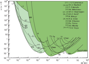
Figure 1: A review of current constraints based on the Yukawa parametrization (1) for deviation from Newton’s law. From Ref. Murata and Tanaka (2015).

The Yukawa parametrization is the most commonly used parametrization for testing for deviations from Newton’s law on sub-mm scales. It is generic and well motivated theoretically as it is a natural prediction in the context of a wide range of modified gravity theories including Brans-Dicke Perivolaropoulos (2010); Hohmann et al. (2013); Järv et al. (2015), scalar-tensor Esposito-Farese and Polarski (2001); Gannouji et al. (2006); Faraoni (2004); Chiba (2003a) and $f(R)$ theories Berry and Gair (2011); Capozziello et al. (2009); Schellstede (2016). It is also a natural prediction of theories involving compactified extra dimensions such as Kaluza-Klein theories Perivolaropoulos (2003).

For example, consider a generic form of $f(R)$ theories with an $R^{2}$ correction of the form Chiba (2003a)

$$f(R)=R+\frac{1}{6m^{2}}R^{2}$$ (3)

The generalized Einstein-Hilbert action is of the form

$$S_{R}=\frac{1}{16\pi G}\int d^{4}x\sqrt{-g}f(R)+S_{matter}$$ (4)

Varying action (4) with respect to the metric leads to the dynamical equations

$$f^{\prime}(R)R_{\mu\nu}-\frac{1}{2}g_{\mu\nu}f(R)=8\pi GT_{\mu\nu}+\nabla_{\mu}\nabla_{\nu}f^{\prime}(R)-g_{\mu\nu}\Box f^{\prime}(R)$$ (5)

Assuming that $f(R)$ has the form of Eq. (3), in the weak field limit $g_{\mu\nu}=\eta_{\mu\nu}+h_{\mu\nu}$, it is straightforward to show that a solution for the metric perturbation $h_{00}$ in the presence of a point mass $M$ takes the form Perivolaropoulos (2017)

$$h_{00}=\frac{2GM}{r}\left(1+\frac{1}{3}e^{-mr}\right)$$ (6)

which compared to the usual Newtonian case has the correction factor $\frac{1}{3}e^{-mr}$. A comparison with the Yukawa ansatz (2) implies that $\alpha=\frac{1}{3}$. A similar form of modified Newtonian force is obtained for massive Brans-Dicke (BD) theories Perivolaropoulos (2017) and for Kaluza-Klein theories Perivolaropoulos and Sourdis (2002); Perivolaropoulos (2003). In those cases the phenomenological parameters $\alpha$, $m$ depend on the fundamental parameters of the theories (e.g. mass of scalar field, Brans-Dicke parameter $\omega$, size and number of extra dimensions).

The above Yukawa parametrization is well motivated theoretically and is currently the standard parametrization used to fit experimental residuals of the Newtonian force. However, alternative parametrizations may also be theoretically motivated in the context of other theoretical models and they may in fact provide better fits to experimental residuals with respect to the Newtonian force on sub-mm scales. For example some brane theories favor a power law residual parametrization Donini and Marimón (2016); Benichou and Estes (2012); Bronnikov et al. (2006); Nojiri and Odintsov (2002). A purely phenomenological approach could also consider arbitrary parametrizations (e.g. spatially oscillating parametrizations) of residual forces designed so that they provide the best fit to residual force data.

Stability of the theories that lead to a Yukawa type of modified Newton’s law usually implies that $m^{2}>0$ Perivolaropoulos (2017). The case $m^{2}<0$ is usually associated with instabilities Faraoni (2006a); Dolgov and Kawasaki (2003) of the underlying theories and also with an oscillating behaviour of the additional term modifying the Newtonian gravitational force. Despite the fact that in these cases we may have no Newtonian limit, such a spatially oscillating term can escape detection if its spatial wavelength is smaller than a fraction of a $mm$ Perivolaropoulos (2017). This case will be discussed in Section III along with an example of a healthy theory (nonlocal gravity Edholm et al. (2016); Kehagias and Maggiore (2014); Frolov and Zelnikov (2016)) that predicts such spatial oscillations without the presence of ghosts/instabilities Tomboulis (1997); Siegel (2003); Biswas et al. (2014).

On the other frontier of testing GR, cosmological scales, the properties of the gravitational theory can be probed by measuring the growth rate of cosmological perturbations through the measurement of peculiar velocities of galaxies (obtained using Redshift Space Distortion (RSD) data Macaulay et al. (2013); Alam et al. (2017)) and through weak gravitational lensing Joudaki et al. (2018); Amon et al. (2017); Abbott et al. (2018). In the presence of perturbations, the perturbed metric in the Newtonian gauge takes the form

$$ds^{2}=-(1+2\phi)dt^{2}+a^{2}(1-2\psi)d{\vec{x}}\,^{2}$$ (7)

where $\phi$ and $\psi$ are potentials with $\phi$ corresponding to the Newtonian potential. These two potentials in general obey modified Poisson equations of the following form

$$\nabla^{2}\phi = 4\pi G_{\rm eff}a^{2}\rho\,\delta_{m},$$ (8)

$$\nabla^{2}(\phi+\psi) = 8\pi G_{L}a^{2}\rho\,\delta_{m},$$ (9)

where $\delta_{m}$ in the linear matter overdensity, $\rho$ is the mean matter density and $a$ is the cosmic scale factor. The potential $\phi$ can be probed using growth of density perturbations observations through RSD data Macaulay et al. (2013); Alam et al. (2017) and $\phi+\psi$ is usually probed using weak lensing data Joudaki et al. (2018); Amon et al. (2017); Abbott et al. (2018). In Eq. (8) and Eq. (9) we also have the parameters $G_{\rm eff}$ and $G_{L}$ which in GR are equal and constant

$$G_{\rm eff}=G_{L}=G_{N}$$ (10)

while in modified gravity theories they can be spacetime dependent. Therefore a basic question arises. “How can the actual data constrain possible scale or redshift dependence of these parameters?”. Here we focus on the $G_{\rm eff}$ that is associated with the Newtonian potential $\phi$ and can be constrained using RSD data measuring the growth of density perturbations.

Early hints of modifications of GR are most likely to come from experiments/observations at the frontier scales: sub-mm and cosmological scales. Important questions that need to be addressed in this context are the following:

• Is GR consistent with currently available data on each scale?

• Even if it is consistent what is the optimum parametrization of the effective Newton’s constant $G_{\rm eff}$ in providing the best quality of fit to the data?

• If there is such parametrization providing a better fit to the data, then what are the theoretical models that support it?

These questions will be the focus of the present brief review.

The structure of this review is the following: In Section II, we focus on cosmological scales and review the phenomenological predictions of modified gravity theories on the observable growth rate of matter density perturbations which can be used as a probe of gravitational physics on cosmological scales. We also focus on Redshift Space Distortions (RSD) as a probe of the growth of matter density perturbations and use an extended compilation of RSD data to identify the tension level between the $\Lambda$CDM parameter values favoured by Planck 2015 Ade et al. (2016) and the corresponding parameter values favoured by the RSD growth data. The effect of an evolving with redshift $z$ effective Newton’s constant $G_{\rm eff}(z)$ on the level of this tension is reviewed and the qualitative features of the best fit form of $G_{\rm eff}(z)$ are identified. The consistency of these qualitative features with specific modified gravity theories is also discussed. In Section III we focus on sub-mm scales and identify the quality of fit of a novel oscillating residual force parametrizations on the data of the Washington small scale gravity experiment. The consistency of this parametrization with specific modified gravity models ($f(R)$ theories and nonlocal gravity) is also discussed. Finally, in Section IV we conclude, summarize and discuss interesting extensions of the reviewed research.

II Hints of Modified Gravity on Cosmological Scales

II.1 RSD Data: Analysis and Phenomenological Implications

A particularly useful probe of the growth rate of density perturbations is weak lensing Joudaki et al. (2018); Amon et al. (2017); Abbott et al. (2018). Recent $\Lambda$CDM parameter constraints emerging from a tomographic weak gravitational lensing analyses indicates a 2-3 $\sigma$ tension in the $\sigma_{8}-\Omega_{m}$ parameter space between the parameter values favoured by Planck 2015 Ade et al. (2016) (which can be seen in Table 1) and specific weak lensing survey data Joudaki et al. (2018); Abbott et al. (2017b).

Table 1: The Planck15/$\Lambda$CDM parameters as reported in Ref. Ade et al. (2016)

Parameter	Planck15/$\Lambda$CDM Values Ade et al. (2016)
$\Omega_{b}h^{2}$	$0.02225\pm 0.00016$
$\Omega_{c}h^{2}$	$0.1198\pm 0.0015$
$n_{s}$	$0.9645\pm 0.0049$
$H_{0}$	$67.27\pm 0.66$
$\Omega_{m}$	$0.3156\pm 0.0091$
$w$	$-1$
$\sigma_{8}$	$0.831\pm 0.013$

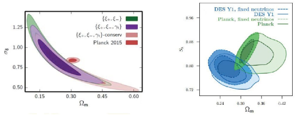
Figure 2: A review of current constraints of weak lensing data with Planck15/$\Lambda$CDM. The left figure corresponds to the Kilo Degree Survey (KiDS) Joudaki et al. (2018) and the right one to the Dark Energy Survey (DES) Abbott et al. (2017b) where $S_{8}\equiv\sigma_{8}\left(\frac{\Omega_{m}}{0.3}\right)^{0.5}$

This tension is demonstrated in Fig. 2. On the left panel we show the $1-2\sigma$, $\sigma_{8}-\Omega_{m}$ best fit parameter contours obtained by the Kilo Degree Survey (KiDS) Joudaki et al. (2018) superposed with the corresponding Planck 2015 Ade et al. (2016) contours. On the right panel we show the $1-2\sigma$, $S_{8}-\Omega_{m}$ ($S_{8}\equiv\sigma_{8}\left(\frac{\Omega_{m}}{0.3}\right)^{0.5}$) best fit parameter contours obtained by the Dark Energy Survey (DES) Abbott et al. (2017b) superposed with the corresponding Planck 2015 Ade et al. (2016) contours. In both cases a $2-3\sigma$ tension between the Planck15/$\Lambda$CDM best fit and the weak lensing best fit parameter values is evident. This tension may be either due to systematics of the weak lensing or Planck15/$\Lambda$CDM data or could be an early hint of new gravitational physics since the weak lensing data are much more sensitive to the growth of cosmological perturbations (gravitational physics) than the CMB data which only probe this growth rate through the ISW effect on very large scales (low $l$).

As is clearly seen from Fig. 2 weak lensing data appear to favour a lower value for $\Omega_{m}$ compared to the value of $\Omega_{m}$ favoured by Planck15/$\Lambda$CDM. The requirement of lower $\Omega_{m}$ favoured by the weak lensing data may also be viewed as a requirement of weaker gravity than implied by GR (Planck15/$\Lambda$CDM) at low redshifts. An interesting question therefore emerges: “Is the same trend for weaker gravity at low redshifts and tension with Planck15/$\Lambda$CDM also favoured by other probes of the growth rate of density perturbation like the RSD data?”

The RSD surveys probe the growth of matter density perturbations by detecting the distortion of the power spectrum of perturbations which are induced by peculiar velocities. This distortion probes the peculiar velocities of galaxies on large scales which in turn can be used to obtain the growth rate of perturbations $f(a)=\frac{dln\delta}{dlna}$, where $a$ is the scale factor and $\delta(a)\equiv\delta\rho/\rho$ is the linear matter overdensity growth factor. Combined with density rms fluctuations within spheres of radius $R=8h^{-1}Mpc$ which may be wriiten as $\sigma_{8}(a)=\sigma_{8}\frac{\delta(a)}{\delta(1)}$, the observable product $f\sigma_{8}(a)$ measured by RSD surveys at various redshifts $z$ (or values of the scale factor $a$) may be expressed in terms of the present value of $\sigma_{8}(a=1)\equiv\sigma_{8}$ and the derivative of $\delta(a)$ with respect to the scale factor $a$ as

$${\rm{\it f\sigma}}_{8}(a) \equiv f(a)\cdot\sigma(a)=\frac{\sigma_{8}}{\delta(1)}~{}a~{}\delta^{\prime}(a)$$ (11)

This combination, i.e. Eq.(11), at various redshifts is published by various surveys as a probe of the growth of matter density perturbations.

Given the background expansion rate $H(z)$ which can be parametrized as $wCDM$

$$E(a)^{2} \equiv \frac{H(a)^{2}}{H_{0}^{2}}=\Omega_{m}a^{-3}+\left(1-\Omega_{m}\right)a^{-3(1+w)}$$ (12)

the theoretically predicted functional form of $\delta(a)$ and therefore of $f\sigma_{8}(a)$ can be obtained on sub-Hubble scales by solving the dynamical growth equation Nesseris et al. (2017)

$$\delta^{\prime\prime}(a)+\left(\frac{3}{a}+\frac{H^{\prime}(a)}{H(a)}\right)\delta^{\prime}(a)-\frac{3}{2}\frac{\Omega_{m}G_{\rm eff}(a,k)/G_{\textrm{N}}}{a^{5}H(a)^{2}/H_{0}^{2}}~{}\delta(a)=0$$ (13)

or in redshift space

$$\delta^{\prime\prime}+\left[\frac{(H^{2})^{\prime}}{2~{}H^{2}}-{\frac{1}{1+z}}\right]\delta^{\prime}={\frac{3}{2}}(1+z)\frac{H_{0}^{2}}{H^{2}}{\frac{G_{\rm eff}(z,k)}{G_{N}}}~{}\Omega_{m}\delta$$ (14)

In Eqs. (13), (14) possible deviations from GR are expressed by allowing for a scale and redshift-dependent effective Newton’s constant $G_{\rm eff}=G_{\rm eff}(a,k)$. It should be stressed that an observed value of $G_{\rm eff}$ that is not constant and/or differs from the Newton’s constant value $G_{N}$ on solar system scales does not necessarily mean that GR is violated. It could also mean that dark energy clusters on sub-Hubble scales and/or that there is a coupling between dark matter and dark energy. Both of these effects would lead to a modification of Eq. (13) from its standard form with $G_{\rm eff}=G_{N}$.

In the context of standard GR ($G_{\rm eff}=G_{N}$) and assuming a $wCDM$ background (12) it is straightforward to solve Eq. (13) numerically with initial conditions deep in the matter era ($\delta(a)\sim a$) and obtain the solution $\delta(a,w,\Omega_{m})$ and then use (11) to obtain the theoretically predicted form of $f\sigma_{8}(a,\sigma_{8},w,\Omega_{m})$ in the context of GR. A fit of this theoretical prediction to the observed RSD datapoints $f\sigma_{8}(z_{i})$ can lead to constraints on the parameters $\sigma_{8},w,\Omega_{m}$. The comparison of these constraints with the corresponding Planck15/$\Lambda$CDM constraints can be a measure of the consistency of the RSD data with Planck15/$\Lambda$CDM in the context of GR.

A fit along the above lines has been implemented in Refs. Nesseris et al. (2017); Kazantzidis and Perivolaropoulos (2018) where $\chi^{2}$ was constructed by defining the vector

$$V^{i}(z_{i},\Omega_{m},\sigma_{8},g_{a})\equiv f\sigma_{8i}-f\sigma_{8}(z_{i},\sigma_{8},w,\Omega_{m})$$ (15)

where $f\sigma_{8i}$ are the RSD datapoints and $f\sigma_{8}(z_{i},\sigma_{8},w,\Omega_{m})$ is the theoretical prediction at the same redshift $z_{i}$. The best fit $\sigma_{8},w,\Omega_{m}$ parameter values were obtained Nesseris et al. (2017); Kazantzidis and Perivolaropoulos (2018) by minimizing

$$\chi^{2}(\sigma_{8},w,\Omega_{m})=V^{i}C_{ij}^{-1}V^{j}$$ (16)

where $C_{ij}$ is the covariance matrix assumed to be diagonal except of the WiggleZ survey $3\times 3$ subset Blake et al. (2012). Thus, the covariance matrix may be written as

$$C_{ij}^{\textrm{growth,total}}=\left(\begin{array}[]{cccc}\sigma_{1}^{2}&0&0&\cdots\\ 0&C_{ij}^{WiggleZ}&0&\cdots\\ 0&0&\cdots&\sigma_{N}^{2}\\ \end{array}\right)$$ (17)

where Blake et al. (2012)

$$C_{ij}^{\text{WiggleZ}}=10^{-3}\left(\begin{array}[]{ccc}6.400&2.570&0.000\\ 2.570&3.969&2.540\\ 0.000&2.540&5.184\\ \end{array}\right)$$ (18)

The rest of the non-diagonal terms are assumed to be 0, implying no correlation among the corresponding datapoints. This assumption is an approximation which as discussed below using Monte Carlo simulations has a relatively small effect on the derived best fit parameter values Kazantzidis and Perivolaropoulos (2018).

A wide range of ${\rm{\it f\sigma}}_{8}$ datasets have been used to constrain cosmological model parameters. Three of the largest such compilations have been constructed in Refs. Nesseris et al. (2017); Kazantzidis and Perivolaropoulos (2018). In Ref. Nesseris et al. (2017) a compilation of 34 ${\rm{\it f\sigma}}_{8}$ datapoints was constructed including datapoints published until 2016. In an attempt to minimize correlations among datapoints a second compilation consisting of 18 ${\rm{\it f\sigma}}_{8}$ datapoints was constructed which included those datapoints that appeared to have minimal levels of correlation (originating from different redshift surveys and different patches in the sky). This more robust compilation is shown in Table LABEL:tab:fs8-data-gold in Appendix A. The third more recent compilation Kazantzidis and Perivolaropoulos (2018) is the largest ${\rm{\it f\sigma}}_{8}$ dataset published to date consisting of $63$ distinct datapoints (Table LABEL:tab:fs8-data-kazan in Appendix A). Despite the possible correlations among the datapoints of this compilation, it contains interesting useful information which has been extracted in the detailed analysis of Ref. Kazantzidis and Perivolaropoulos (2018).

The growth rate of cosmological perturbations is obtained from the RSD data by comparing the observed power spectrum of large scale structures in redshift space $P_{obs}(k_{ref\perp},k_{ref\parallel},z)$ with the expected isotropic (due to the cosmological principle) true underlying spectrum $P_{matter}(k,z)\sim\delta\rho/\rho(k,z)^{2}$ where $k_{ref\parallel}$ is the Fourier scale wavevector component parallel to the line of sight and $k_{ref\perp}$ is the corresponding wavevector perpendicular to the line of sight in the context of a given reference (fiducial) cosmology used to convert the measured angles and redshifts to distances. The true statistically isotropic power spectrum depends only on the magnitude of the true Fourier scale wavevector. The observed spectrum of perturbations is distorted for two reasons:

• Incorrect Fiducial Cosmology: The redshift surveys measure galaxy redshifts and angles of galaxies. In order to construct the correlation function and thus the power spectrum, these angles and redshifts need to be converted to comoving coordinates. This conversion requires the assumption of a particular form of $H_{ref}(z)$ (a reference or fiducial cosmology) which is not necessarily identical with the true cosmology $H(z)$. The use of an incorrect fiducial cosmology $H_{ref}(z)$ would lead to an incorrect distorted nonisotropic power spectrum $P_{obs}(k_{ref\perp},k_{ref\parallel},z)$ which may be shown Alam et al. (2016); Hinton (2016) to be connected with the galaxy power spectrum $P_{g}(k_{ref\perp},k_{ref\parallel},z)$ obtained with the correct cosmology $H(z)$ with the relation Alam et al. (2016)

  $$P_{obs}(k_{ref\perp},k_{ref\parallel},z)=\frac{d_{A}(z)^{2}_{{}_{ref}}H(z)}{d_{A}(z)^{2}H_{ref}(z)}P_{g}(k_{ref\perp},k_{ref\parallel},z)$$ (19)

  where $d_{A}(z)$ is the angular diameter distance. This geometric distortion of the correlation function and the power spectrum due to the use of the incorrect fiducial cosmology is known as the Alcock-Paczynski (AP) effect.

  Even if the correct cosmology was used for the conversion of angles-redshifts to distances, the power spectrum $P_{g}$ is still nonisotropic. The reason for this remaining distortion are the peculiar velocities of galaxies which encapsulate the information for the gravitational growth of perturbation. Thus, the second effect that distorts the observed power spectrum is the peculiar velocity effect.

• Peculiar Velocities: Peculiar velocities add an extra component to the cosmological redshifts thus perturbing the real positions of galaxies $x_{r}$ along the line of sight to a new position $x_{p}$ of the form Ballinger et al. (1996); Amendola et al. (2018)

  $$x_{p}=x_{r}+(1+z)\frac{{\hat{x}}\cdot{\vec{v}}}{H(z)}$$ (20)

  This distortion of galaxy positions due to their peculiar velocities leads to an additional distortion of the observed power spectrum of the form

  $$P_{g}(k_{ref\perp},k_{ref\parallel},z)=b(z)^{2}\left[1+\beta(z)\frac{k_{ref\parallel}^{2}}{k_{ref\parallel}^{2}+k_{ref\perp}^{2}}\right]^{2}\;P_{matter}(k,z)$$ (21)

  where $b(z)$ is the bias factor (the ratio of the galaxy overdensities over the underlying matter overdensities) and $\beta(z)\equiv\frac{f(z)}{b(z)}$ is the linear redshift space distortion parameter. The wavenumbers $k_{ref\perp}$ and $k_{ref\parallel}$ obtained using the fiducial cosmology are connected to the wavenumbers $k_{\parallel}$ and $k_{\perp}$ in the true cosmology as $k_{ref\parallel}=\frac{H_{ref}(z)}{H(z)}k_{\parallel}$, $k_{ref\perp}=\frac{d_{A}(z)}{d_{Afid}(z)}k_{\perp}$. Using Eq. (21), the measured distorted power spectrum $P_{g}(k_{ref\perp},k_{ref\parallel},z)$ and the isotropy of the true power spectrum, the parameter $\beta(z)$ can be inferred and from it the bias free product ${\rm{\it f\sigma}}_{8}$ can be derived.

Each one of the datapoints of Tables LABEL:tab:fs8-data-kazan and LABEL:tab:fs8-data-gold is constructed under the assumption of a particular fiducial cosmology. Thus an Alcock-Paczynski correction factor needs to be imposed to each one of the datapoints converting them to the values corresponding to the true cosmology $H(z)$. If an ${\rm{\it f\sigma}}_{8}^{\prime}$ measurement has been obtained assuming a fiducial $\Lambda$CDM cosmology $H^{\prime}(z)$, the corresponding ${\rm{\it f\sigma}}_{8}$ obtained with the true cosmology $H(z)$ is approximated as Macaulay et al. (2013)

$$f\sigma_{8}(z)\simeq\frac{H(z)d_{A}(z)}{H^{\prime}(z)d_{A}^{\prime}(z)}f\sigma_{8}^{\prime}(z)\equiv q(z,\Omega_{m},\Omega_{m}^{\prime})\;f\sigma_{8}^{\prime}(z)$$ (22)

This equation should be taken as a rough order of magnitude estimate of the AP effect as it appears in somewhat different forms in the literature Saito (2016); Wilson (2016); Alam et al. (2016).

This correction is small (at most it can be about $2-3\%$ at redshifts $z\simeq 1$ for reasonable values of $\Omega_{m}$) Kazantzidis and Perivolaropoulos (2018). The magnitude of this factor is demonstrated in Fig. 3 for typical values of fiducial and true cosmologies.

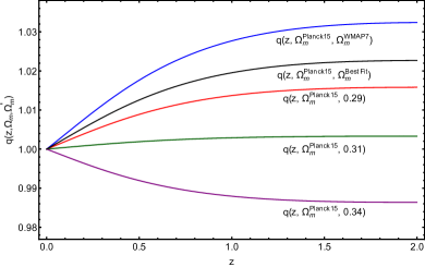
Figure 3: Plot of the correction factor $q$ as a function of the redshift $z$ (from Ref. Kazantzidis and Perivolaropoulos (2018))

The fiducial model corrected dataponts of Tables LABEL:tab:fs8-data-kazan and LABEL:tab:fs8-data-gold are shown in Figs. 4 and 5, respectively along with the predictions of specific models obtained by solving Eq. (14) with matter domination initial conditions and using Eq. (11) for specific cosmological models: Planck15/$\Lambda$CDM with GR ($G_{\rm eff}=G_{N}$), the best fit $\Lambda$CDM model to the ${\rm{\it f\sigma}}_{8}$ data (with a reduced value of $\Omega_{m}$) and a modified gravity model where the background expansion is given by the Planck15/$\Lambda$CDM parameters while $G_{\rm eff}$ is allowed to vary with redshift with a specific

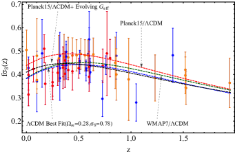
Figure 4: Plot of ${\rm{\it f\sigma}}_{8}$ as a function of the redshift $z$ for the full growth rate data set of Table LABEL:tab:fs8-data-kazan in Appendix A. The green dashed line describes the best fits of WMAP7/$\Lambda$CDM while the red one the best fits of Planck15/$\Lambda$CDM. The blue dashed line describes the best fit $\Lambda$CDM ($\Omega_{m}=0.28\pm 0.02$) indicated by Table LABEL:tab:fs8-data-kazan while the black one corresponds to an evolving $G_{\rm eff}(z)$ parametrization with a Planck15/$\Lambda$CDM background. The 20 earlier published data from the compilation are denoted as red points whereas the 20 latest published points are denoted as orange points (from Ref. Kazantzidis and Perivolaropoulos (2018))

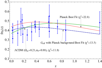
Figure 5: Plot of ${\rm{\it f\sigma}}_{8}$ as a function of the redshift $z$ for the 18 growth rate dataset of Ref. Nesseris et al. (2017). The green dashed line describes the best fit of $\Lambda$CDM ($\Omega_{m}=0.21$), the red one the best fit of Planck15/$\Lambda$CDM. The blue dot-dashed one corresponds to an evolving $G_{\rm eff}(z)$ parametrization with a Planck15/$\Lambda$CDM background.

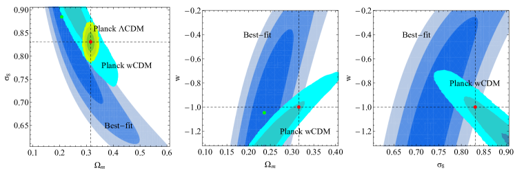
Figure 6: The $1\sigma-3\sigma$ contours level in the parametric space $(w,\sigma_{8},\Omega_{m})$ using the collection of the 18 points presented in Ref. Nesseris et al. (2017). The blue contours describe the best fit of the data, the light green contours correspond to Planck15/$\Lambda$CDM while the light blue are constructed from the Planck data assuming a $wCDM$ background.

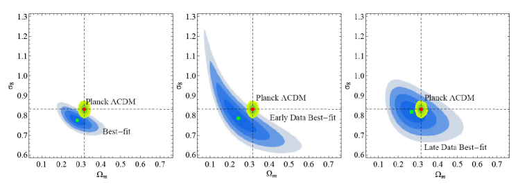
Figure 7: The $1\sigma-4\sigma$ confidence contours in the parametric space $(\Omega_{m}-\sigma_{8})$ using the full dataset of ${\rm{\it f\sigma}}_{8}$ (Table LABEL:tab:fs8-data-kazan) from Ref. Kazantzidis and Perivolaropoulos (2018). The blue contours correspond to the best fit obtained using the full compilation of ${\rm{\it f\sigma}}_{8}$ data from Table LABEL:tab:fs8-data-kazan (left panel), the 20 early data (middle panel) and the 20 late data (right panel). The light green contours describe the contours for the Planck15/$\Lambda$CDM model.

parametrization described below so that the best fit to the ${\rm{\it f\sigma}}_{8}$ data is obtained. In both Figs. 4 and 5 it is clear that the Planck15/$\Lambda$CDM prediction (red dashed line) is somewhat higher than the majority of the ${\rm{\it f\sigma}}_{8}$ datapoints indicating that the growth rate is too large in this model. As shown in Figs. 4 and 5, this growth rate at low $z$ can be reduced (thus improving the fit to the data) by either decreasing $\Omega_{m}$ while maintaining GR and $\Lambda$CDM (green line) or by allowing for a $G_{\rm eff}$ that evolves with redshift so that it is reduced at low $z$ (blue line). As a result, the growth data at low redshifts $(z<1)$ are more appropriate to detect possible deviations from GR than the points at high redshifts $(z>1)$ Kazantzidis et al. (2019).

The tension between a Planck15/$\Lambda$CDM background (GR) and the growth data of Fig. 5 is shown more clearly in Fig. 6 where we show the likelihood contours in two dimensional subspaces of the parameter space $\sigma_{8},w,\Omega_{m}$. In each plot, the third parameter has a fixed value indicated by Planck15/$\Lambda$CDM.

The blue $1\sigma-2\sigma$ parameter contours are obtained using the growth data of Fig. 5 while the red dot corresponds to the Planck15/$\Lambda$CDM. Clearly, there is a $2-3\sigma$ tension between the growth data contours and the best fit Planck15/$\Lambda$CDM parameter values. The Planck15 best fit $wCDM$ parameter contours are also shown indicating that if the equation of state parameter $w$ is allowed to vary, the tension level between the growth data parameter $1\sigma-2\sigma$ contours (blue contours) and the Planck15 Ade et al. (2016) contours is significantly reduced.

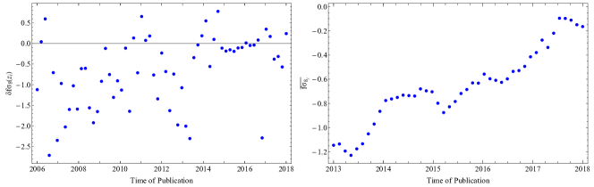
Figure 8: Left panel: Residuals datapoints vs time of publication. Right panel: The 20 points moving average vs time of publication (from Ref. Kazantzidis and Perivolaropoulos (2018)).

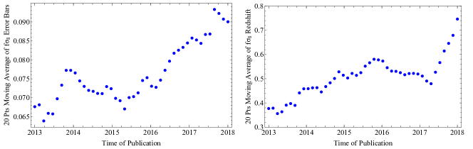
Figure 9: Left panel: The 20 point moving average of the growth error bars with time of publication. Right panel: The 20 point moving average of the redshifts of ${\rm{\it f\sigma}}_{8}$ redshifts with time of publication (from Ref. Kazantzidis and Perivolaropoulos (2018))

An interesting question to address is the following: “How does the level of tension between the growth data and the Planck15/$\Lambda$CDM best fit parameter values evolve with time of publication?” or “Are early growth data at the same tension level with Planck15/$\Lambda$CDM as more recently published data?” This question has been addressed in Ref. Kazantzidis and Perivolaropoulos (2018) using the data of Table LABEL:tab:fs8-data-kazan and reviewed in what follows.

The evolution of the tension level is demonstrated in Fig. 7 where we show the ($\Omega_{m}-\sigma_{8}$) $\Lambda$CDM ($w=-1$) best fit parameter contours obtained with the full dataset of Table LABEL:tab:fs8-data-kazan (left panel), with the earliest 20 datapoints (middle panel) and with the latest 20 datapoints of the same Table.

Interestingly, the tension drops from a level more than $3\sigma$ for the early published data to less than $1\sigma$ for the $20$ most recent datapoints. The exact tension level ($\sigma$ distance between the growth data best fit parameters and the Planck15/$\Lambda$CDM best fit parameters) is shown in Table 2.

Table 2: The sigma differences of Fig. 7 Contours for the Full Dataset, Early and Late Data.

	Full Dataset	Early Data	Late Data
Fig. 7 Contours	$4.97\sigma$	$3.89\sigma$	$0.94\sigma$

The evolving tension between Planck15/$\Lambda$CDM parameter values and ${\rm{\it f\sigma}}_{8}$ data may also be described by defining the residuals

$$\delta f\sigma_{8}(z_{i})\equiv\frac{f\sigma_{8}(z_{i})^{data}-f\sigma_{8}(z_{i})^{Planck15/\Lambda CDM}}{\sigma_{i}}$$ (23)

Using these residuals, the 20 point moving average residual may be defined as

$$\overline{{f\sigma_{8}}_{j}}\equiv\sum_{i=j-20}^{j}\frac{\delta f\sigma_{8}(z_{i})}{20}$$ (24)

These residual datapoints versus time of publication along with the corresponding 20 point moving average from Eq. (24), are shown in Fig. 8 (from Ref. Kazantzidis and Perivolaropoulos (2018)). There is a clear trend for reduced tension with Planck15/$\Lambda$CDM in more recently published data.

More recent ${\rm{\it f\sigma}}_{8}$ datapoints tend to probe higher redshifts and thus they also tend to have higher errors. This is demonstrated in Fig. 9 where we show the 20 point moving average of the datapoint errorbars and redshifts versus time of publication. Both of them show an increasing trend especially for more recent data. At higher redshifts the universe is matter dominated and GR is approximately restored in most models and thus there is degeneracy in the predictions of different models. Thus, more recent datapoints that tend to probe higher redshifts have less constraining power on cosmological models.

In fact, the increase of the average redshift is a possible explanation for the reduced tension of the recent data with Planck15/$\Lambda$CDM due to the degeneracy that exists between models at high z. This degeneracy can also be observed in Fig. 4, where for high $z$ the four curves coincide.

As discussed above, the tension between ${\rm{\it f\sigma}}_{8}$ data and Planck15/$\Lambda$CDM may be reduced by either reducing $\Omega_{m}$ or by extending GR and allowing for an evolving $G_{\rm eff}$. Such an evolving $G_{\rm eff}(z)$ may be described by a parametrization of the form

$$\frac{G_{\textrm{eff}}(a,g_{a},n)}{G_{\textrm{N}}} = 1+g_{a}(1-a)^{n}-g_{a}(1-a)^{2n}$$ (25)

$$= 1+g_{a}\left(\frac{z}{1+z}\right)^{n}-g_{a}\left(\frac{z}{1+z}\right)^{2n}.$$

where $g_{a}$ and $n$ are parameters to be fit. This parametrization for $n=2$ has been used for the construction of the Figs. 6 and 7.

The parametrization (25) is well motivated and consistent with solar system experiments. The solar system constraints entail for the first derivative that Nesseris and Perivolaropoulos (2007)

$$\lim_{z\to 0}G^{\prime}_{\rm eff}(z)\simeq 0\Rightarrow\Big{\lvert}\frac{1}{G_{N}}\frac{dG_{\rm eff}(z)}{dz}\Big{|}_{z=0}\Big{\rvert}<10^{-3}h^{-1}$$ (26)

This constraint implies that unless a Chameleon type mechanism Khoury and Weltman (2004) is present we must have $n\geq 2$ in the parametrization (25). The solar system experiments also leave the second derivative unconstrained since Nesseris and Perivolaropoulos (2007)

$$\Big{|}\frac{1}{G_{N}}\frac{d^{2}G_{\rm eff}(z)}{dz^{2}}\Big{|}_{z=0}\Big{|}<10^{5}h^{-2}$$ (27)

Finally, at high redshifts, the Big Bang Nucleosynthesis provides the following additional constraint at the $1\sigma$ level Copi et al. (2004)

$$\lvert G_{\rm eff}/G_{N}-1\rvert\leq 0.2$$ (28)

which is also consistent with the parametrization (25).

In the context of this parametrization, which was presented in Refs. Nesseris et al. (2017); Kazantzidis and Perivolaropoulos (2018), two extra parameters have been inserted ($g_{a}$ and $n$) describing the possible deviation from GR. Setting $\Omega_{m}=\Omega_{m}^{Planck15}$ and $\sigma_{8}=\sigma_{8}^{Planck15}$, i.e. eliminating the tension with respect to $\Omega_{m}$ and $\sigma_{8}$, we see that the value of $\chi^{2}$ gets reduced significantly for $g_{a}\neq 0$ (using the data of Table LABEL:tab:fs8-data-gold in the Appendix A and setting $n=2$ it was found that $g_{a}=-1.16\pm 0.341$). This corresponds to the blue curve of Fig. 5. The best fit values of of $g_{a}$ for various values of $n$ are also shown in Table 3 and the corresponding forms of $G_{\rm eff}(z)$ are shown in Fig. 10.

Table 3: The best fit values of $g_{a}$ along with the $1\sigma$ errors bars for various values of $n$.

$n$	$g_{a}$
$0.343$	$-1.200\pm 1.025$
$1$	$-0.944\pm 0.253$
$2$	$-1.156\pm 0.341$
$3$	$-1.534\pm 0.453$
$4$	$-2.006\pm 0.538$
$5$	$-2.542\pm 0.689$
$6$	$-3.110\pm 0.771$

Notice that a significant reduction of the gravitational constant is required at low $z$ to fit the ${\rm{\it f\sigma}}_{8}$ data with $\Omega_{m}=\Omega_{m}^{Planck15}$. Such a large reduction is inconsistent with other cosmological observations (e.g. CMB large scale power spectrum where the ISW effect dominates Nesseris et al. (2017) or the distance moduli of SnIa when their dependence on $G_{\rm eff}(z)$ is taken into account Gannouji et al. (2018)) and therefore it is unlikely that the tension implies only the existence of evolving $G_{\rm eff}(z)$. It is more likely that the tension is also (or only) due to other factors like a reduced value of $\Omega_{m}$ or systematic/statistical errors of the ${\rm{\it f\sigma}}_{8}$ data.

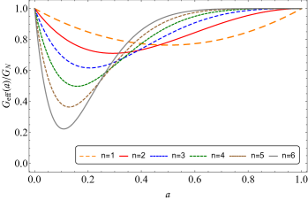
Figure 10: Plot of $G_{\text{eff}}/G_{\text{N}}$ as a function of $a$ considering the values of $n$ and $g_{a}$ from Table 3 (from Ref. Nesseris et al. (2017))

The evolution of the tension level with time of pubication of the ${\rm{\it f\sigma}}_{8}$ data may also be seen by deriving the best fit value of the parameter $g_{a}$ assuming $n=2$ and a Planck15/$\Lambda$CDM background while using 20 datapoint subsamples from Table LABEL:tab:fs8-data-kazan starting from the earliest to the latest subsample (from left to right in Fig. 11).

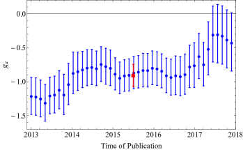
Figure 11: The $1\sigma$ range of the parameter $g_{a}$ from the compilation of Table LABEL:tab:fs8-data-kazan. The red square point denotes the the best fit of $g_{a}$ obtained from the compilation of Table LABEL:tab:fs8-data-kazan along with its error bar (from Ref. Kazantzidis and Perivolaropoulos (2018))

Clearly the absolute value of $g_{a}$ required to eliminate the tension with Planck15/$\Lambda$CDM decreases significantly for more recent data indicating also the reduced level of the tension for more recent data. The best fit value of $g_{a}$ for the full dataset of Table LABEL:tab:fs8-data-kazan ($g_{a}=-0.91\pm 0.17$) is also indicated in Fig. 11 (red point).

II.2 Consistency of Reduced $G_{\rm eff}(z)$ with Modified Gravity Theories

The best fit form of $G_{\rm eff}(z)$ which appears to indicate reduced strength of gravity at low $z$ may lead to constraints on the fundamental parameters of modified theories of gravity. In fact, it may be shown that the simplest modified gravity theories including $f(R)$ and scalar-tensor theories tend to be inconsistent with a decreasing $G_{\rm eff}(z)$ especially in a $\Lambda$CDM and in a phantom cosmological background Gannouji et al. (2018).

In scalar-tensor gravity the action has the following form Esposito-Farese and Polarski (2001); Boisseau et al. (2000)

$${\cal S}=\int d^{4}x\sqrt{-g}\left[\frac{1}{2}F(\phi)R-\frac{1}{2}Z(\phi)g^{\mu\nu}\partial_{\mu}\phi\partial_{\nu}\phi-U(\phi)\right]+S_{m},$$ (29)

where we have set $8\pi G=1$. It is clear from Eq. (29) that the action depends on the scalar field $\phi$. Throughout this subsection we also consider $Z(\phi)=1$. The line element for a flat Friedmann-Robertson-Walker(FRW) metric is

$$ds^{2}=-dt^{2}+a^{2}(t)\left[dr^{2}+r^{2}(d\theta^{2}+\sin^{2}\theta\ d\phi^{2})\right].$$ (30)

By varying the action (29) with respect to the inverse metric, considering that the scalar field is homogenous and that the background is that of a perfect fluid, the dynamical equations of motion are of the following form

$$3FH^{2} = \rho+{\frac{1}{2}}\dot{\phi}^{2}-3H\dot{F}+U$$ (31)

$$-2F\dot{H} = (\rho+p)+\dot{\phi}^{2}+\ddot{F}-H\dot{F}$$ (32)

Usually it is convenient to express Eqs. (31) and (32) in terms of the redshift $z$. We define the squared rescaled Hubble parameter as

$$q(z)\equiv E^{2}(z)=\frac{H^{2}(z)}{H_{0}^{2}}$$ (33)

After an additional rescaling of the potential ($U\rightarrow U\cdot H_{0}^{2}$) the equation of motion for $F(z)$ is Esposito-Farese and Polarski (2001); Boisseau et al. (2000); Nesseris et al. (2017)

$$F^{\prime\prime}(z)+\left[\frac{q^{\prime}(z)}{2q(z)}-\frac{2}{1+z}\right]F^{\prime}(z)-\frac{1}{(1+z)}\frac{q^{\prime}(z)}{q(z)}F(z)+3\frac{1+z}{q(z)}\Omega_{m}=-\phi^{\prime}(z)^{2}$$ (34)

where the prime denotes from now on differentiation with respect to $z$.

In scalar-tensor theories the effective Newton’s constant may be expressed as Nesseris and Perivolaropoulos (2006)

$$G_{\rm eff}(z)/G_{\textrm{N}}=\frac{1}{F(z)}\frac{F(z)+2F_{,\phi}^{2}}{F(z)+\frac{3}{2}F_{,\phi}^{2}}$$ (35)

where $G_{\text{N}}$ is the usual Newton’s constant in GR.

Using the best fit form of $G_{\rm eff}(z)$ on the left hand side of Eq. (35), we may obtain the corresponding form of $F(z)$ and then use Eq. (34) with a $q(z)$ corresponding to Planck15/$\Lambda$CDM to find the corresponding form of $\phi^{\prime}(z)^{2}$. Therefore the question that we want to address is: “Can the weakening effect of gravity indicated by the growth data be due to an underlying scalar-tensor theory?”

If this effect is due to an underlying scalar-tensor theory, then the new reconstructed scalar field must obey $\phi^{\prime}(z)^{2}>0$ so that the theory is self consistent. However a decreasing $G_{\textrm{eff}}$ with redshift at low $z$ is inconsistent with $\phi^{\prime}(z)^{2}>0$ as it is demonstrated numerically in the following Fig. 12.

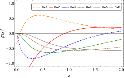
Figure 12: Plot of $\phi^{\prime}(z)^{2}$ with redshift $z$ for various values of $n$ (from Ref. Nesseris et al. (2017)). The best fit values of $g_{a}$ shown in Table 3 were assumed with a Planck15/$\Lambda$CDM background.

From Fig. 12 it is clear that at low $z$, $\phi^{\prime}(z)^{2}$ is negative. As a result this behaviour can not be supported by a self consistent scalar tensor theory.

This numerical result may also be demonstrated analytically. For a wCDM background we have

$$q(z)=\Omega_{m}(1+z)^{3}+\left(1-\Omega_{m}\right)(1+z)^{3(1+w)}$$ (36)

For low $z$, we can expand the dynamical Newton’s constant $G_{\rm eff}(z)$, which up to the second order is of the form

$$G_{\rm eff}(z)=G_{\rm eff}(0)+G^{\prime}_{\rm eff}(0)z+\frac{z^{2}}{2}G^{\prime\prime}_{\rm eff}(0)$$ (37)

Applying the solar system constraints for the first derivative of $G_{\rm eff}(z)$, i.e. Eq. (26), Eq. (37) is rewritten as

$$G_{\rm eff}(z)=G_{\rm eff}(0)+\frac{z^{2}}{2}G^{\prime\prime}_{\rm eff}(0)$$ (38)

It is straightforward to show that the constraint of Eq. (26) implies that $F^{\prime}(0)\approx 0$. Therefore, setting $G_{N}=F(0)=1$ and differentiating $G_{\rm eff}(z)$ with respect to $z$ we obtain

$$G_{\rm eff}^{\prime\prime}(0)=F^{\prime\prime}(0)\left(-1+\frac{F^{\prime\prime}(0)}{\phi^{\prime}(0)^{2}}\right)$$ (39)

Furthermore, using Eq. (36) in Eq. (39) and setting $z=0$, Eq. (40) is derived

$$3-3w(-1+\Omega_{0m})-3\Omega_{0m}-\phi^{\prime}(0)^{2}-F^{\prime\prime}(0)=0$$ (40)

Substituting it to Eq. (39), the second derivative of $G_{\rm eff}(z)$ takes the following form Gannouji et al. (2018)

$$G_{\rm eff}^{\prime\prime}(0)=9(1+w)(-1+\Omega_{m})+\frac{9(1+w)^{2}(-1+\Omega_{m})^{2}}{\phi^{\prime}(0)^{2}}+2\phi^{\prime}(0)^{2}$$ (41)

Fixing a $\Lambda$CDM background, i.e. setting $w=-1$, Eq. (37) takes the form

$$G_{\rm eff}(z)\approx G_{\rm eff}(0)+\frac{1}{2}G_{\rm eff}^{\prime\prime}(0)z^{2}=G_{\rm eff}(0)+\phi^{\prime 2}(0)z^{2}$$ (42)

which is always an increasing function of $z$ if we assume that the kinetic term of $\phi^{\prime}(z)$ is always positive, an assumption which is crucial if we want to have a self-consistent theory. This is demonstrated in Fig. 13.

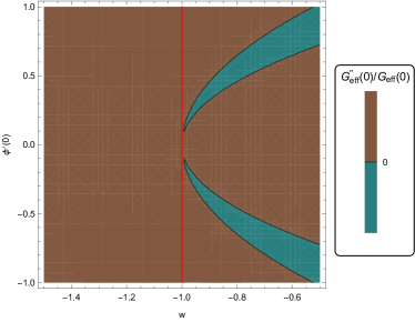
Figure 13: The second derivative of $G_{\rm eff}$ in the parametric space $(\phi^{\prime}(0)-w)$, setting $\Omega_{m}=0.3$. With blue we denote the parameter values in which $G_{\rm eff}^{\prime\prime}(0)<0$, while the brown regions describes $G_{\rm eff}^{\prime\prime}(0)>0$ which is achieved only for $w>-1$.

From the above analysis the following result is extracted: If a $\Lambda$CDM background is assumed, any $G_{\rm eff}(z)$ initially decreasing with $z$ leads to a reconstructed scalar-tensor negative kinetic term for some range of low $z$ Gannouji et al. (2018).

Since the magnitude of the best fit parameter $g_{a}$ is relatively large, it is important to test its consistency with other observational probes and in particular with the low $l$ angular power spectrum of the CMB which is affected by the ISW effects and therefore can probe the strength of gravity. Using MGCAMB Hojjati et al. (2011) the predicted CMB angular power spectrum may be derived assuming a Planck15/$\Lambda$CDM background cosmology and a $G_{\rm eff}(z)$ parametrized by the ansatz (25). Such an analysis Nesseris et al. (2017) indicates that for $l\raisebox{-3.69899pt}{~{}\shortstack{$>$ \\ [-0.07cm] $\sim$}}~{}80$ the CMB angular power spectrum remains practically unaffected by the evolving form of $G_{\rm eff}(z)$ and thus the Planck15/$\Lambda$CDM best fit parameter value for $\Omega_{m}$ remains also practically unaffected. On the other hand, the low $l$ CMB spectrum is affected significantly due to the ISW effect. This is demonstrated in Fig. 14 Nesseris et al. (2017) where the measured low $l$ values of the $C_{l}$ components are superposed with the theoretical prediction obtained for an evolving $G_{\rm eff}(z)$ for various values of the parameters $g_{a}$ and $n$.

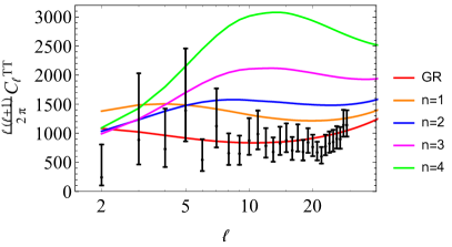
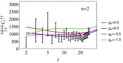
Figure 14: Top panel: The theoretically predicted CMB power spectra for the best fit parameter values $g_{a}$ for various values of $n$ from Table 3. Clearly these best fit forms of $G_{\rm eff}(z)$ are not consistent with the observed values of $C_{l}^{\prime}s$. Therefore, the tension between the Planck15/$\Lambda$CDM best fit parameter values and those indicated by the ${\rm{\it f\sigma}}_{8}$ data can not be attributed solely to an evolving $G_{\rm eff}(z)$. Bottom panel: The theoretically predicted low $l$ CMB power spectra for $n=2$ and various values of $g_{a}$. Only values $|g_{a}|\lesssim 0.5$ are consistent with the observed CMB power spectrum (from Ref. Nesseris et al. (2017)).

Clearly the low $l$ CMB power spectra impose strong constraints on the allowed values of $g_{a}$ and only the range $|g_{a}|\lesssim 0.5$ appears to be consistent with the observed values of low $l$ $C_{l}^{\prime}s$.

III Hints of Modified Gravity on Sub millimetre Scales

III.1 Review of the Washington Experiment

As discussed in the Introduction, the small scale frontier of the gravitational physics research is on sub-mm scales. This scale, however, is also connected with macrophysics and with dark energy. In fact, the dark energy scale may be written as

$$\lambda_{de}\equiv\sqrt[4]{\hbar c/\rho_{de}}\approx 0.085mm$$ (43)

where it is assumed that $\Omega_{m}=0.3$ and $H_{0}=70kmsec^{-1}Mpc^{-1}$. Hence, if the accelerating expansion is connected with modified gravity, it is natural to expect signatures of modified theories of gravity on scales $\lambda\approx 0.1mm$.

In the last decade a large number of experiments Murata and Tanaka (2015); Kapner et al. (2007a); Hoyle et al. (2004b, 2001) have imposed constraints on parametrizations which are extensions of Newton’s gravitational potential.

One of the most sensitive such experiments which have imposed the best constraints so far on the Yukawa parametrization discussed in the Introduction is the Washington experiment Hoyle et al. (2004a) which consists of three similar setups (Experiments I, II, III). It is based on a torsion-balance set-up shown in Fig. 15.

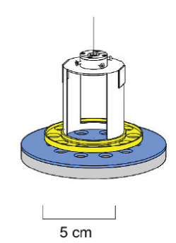
Figure 15: The Washington Experiment set-up (from Ref. Hoyle et al. (2004a))

It consists of a fiber pendulum, 82 cm long, attached to a thin plate ring (yellow in Fig. 15) placed above a rotating plate with holes (blue in Fig. 15). The blue ring was an attractor which, like the pendulum ring, contained ten equally spaced holes with diameters about 9.5mm. The test-bodies used to measure the gravitational interaction were the holes excerting a torque of the form

$$N(\phi)=-\frac{\partial V(\phi)}{\partial\phi}$$ (44)

where $V(\phi)$ is the potential energy of the attractor ring-pendulum system when the holes of the ring twisted and formed an angle $\phi$ with respect to the pendulum.

The torque residuals that were measured in this experiment were fit assuming two different forms of a gravitational potential: A Yukawa parametrization of the form

$$V_{\rm eff}=-G\frac{M}{r}(1+\alpha e^{-mr})$$ (45)

and a power law parametrization of the form Kapner et al. (2007b)

$$V_{\rm eff}=-G\frac{M}{r}\left(1+\beta_{k}\left[\frac{1mm}{r}\right]^{k-1}\right)$$ (46)

This power law ansatz emerges naturally from some brane world models Donini and Marimón (2016); Benichou and Estes (2012); Bronnikov et al. (2006); Nojiri and Odintsov (2002). The torque residuals from the Newtonian torques are shown Fig. 16 along with the predicted residuals in the context of the above generalized gravitational potentials for specific parameter values.

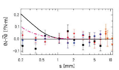
Figure 16: The residuals of the datapoints used in the analysis of Ref. Hoyle et al. (2004a) (datapoints of Experiment I). The solid curve corresponds to residuals of the Yukawa parametrization of Eq. (45) for $a=1$, $m^{-1}=\lambda=250\mu m$, whereas the dot-dashed describes the power law of Eq. (46), where $k=5$ and $\beta_{k}=0.005$ (from Ref. Hoyle et al. (2004a)).

III.2 Yukawa and Oscillating Newtonian Potenial in $f(R)$ Theories

The simplest form of $f(R)$ theories is $f(R)=R+\frac{1}{6m^{2}}R^{2}+...$. In the weak field limit for $m^{2}>0$ the theory is self consistent and stable Berry and Gair (2011); Capozziello et al. (2007) leading to Yukawa type correction to the gravitational potential. For $m^{2}<0$ the Yukawa type gravitational potential gets modified and the exponentially suppressed correction transforms to an oscillating correction of the form

$$V_{\rm eff}=-G\frac{M}{r}(1+\alpha\cos(mr+\theta))$$ (47)

where $\theta$ is a parameter.

In order to demonstrate the validity of the modified Newtonian potentials (45) and (47) in the context of $f(R)$ theories, consider the generalized Einstein-Hilbert action Perivolaropoulos (2017); Starobinsky (2007); De Felice and Tsujikawa (2010)

$$S_{R}=\frac{1}{16\pi G}\int d^{4}x\sqrt{-g}f(R)+S_{matter}$$ (48)

where $R$ is the Ricci scalar. It is easy to show that this action can be rewritten in the equivalent form Chiba (2003b); Faraoni (2006b)

$$S_{BD}=\frac{1}{16\pi G}\int d^{4}x\sqrt{-g}\left[f(\phi)+f_{\phi}(\phi)(R-\phi)\right]+S_{matter}$$ (49)

By varying action (49) with respect to the scalar field $\phi$ and assuming $f_{\phi\phi}\neq 0$ we obtain

$$\phi=R$$ (50)

Setting $f(R)=R+\frac{1}{6m^{2}}R^{2}$, and defining $\Phi\equiv 1+\frac{1}{3m^{2}}\phi$, then it is straightforward to rewrite Eq. (49) as

$$S_{BD}=\frac{1}{16\pi G}\int d^{4}x\sqrt{-g}\left[\Phi R-\frac{3}{2}m^{2}(\Phi-1)^{2}\right]+S_{matter}$$ (51)

which is the action of a massive BD scalar field with $\omega=0$.

Furthermore, varying Eq. (51) with respect to the inverse metric and the scalar field $\Phi$, we obtain the dynamical equations

$$\Phi\left(R_{\mu\nu}-{\frac{1}{2}}g_{\mu\nu}R\right)=8\pi GT_{\mu\nu}+\nabla_{\mu}\partial_{\nu}\Phi-g_{\mu\nu}\Box\Phi-g_{\mu\nu}\frac{3}{4}m^{2}(\Phi-1)^{2}$$ (52)

$$\Box\Phi=\frac{8\pi G}{3}\,T+m^{2}\left((\Phi-1)^{2}+(\Phi-1)\Phi\right)$$ (53)

respectively. Considering the weak gravitational field for a point mass of the form

$$T_{\mu\nu}=diag(M\delta(\vec{r}),0,0,0)$$ (54)

the quantities $\Phi$ and $g_{\mu\nu}$ can be expanded as

$$\Phi = 1+\varphi$$ (55)

$$g_{\mu\nu} = \eta_{\mu\nu}+h_{\mu\nu}$$ (56)

Substituting Eqs. (55) and (56) in the dynamical equations and keeping terms up to linear order we obtain the perturbative dynamical equations around the vacuum solution as

$$\left(\Box-m^{2}\right)\varphi=-\frac{8\pi G}{3}M\delta(\vec{r})$$ (57)

$$-\frac{1}{2}\left[\Box\left(h_{\mu\nu}-\eta_{\mu\nu}\frac{h}{2}\right)\right]=8\pi GT_{\mu\nu}+\partial_{\mu}\partial_{\nu}\varphi-\eta_{\mu\nu}\Box\varphi$$ (58)

where $h=h^{\mu}_{\mu}$. For static configurations, these equations convert to

$$\nabla^{2}\varphi-m^{2}\varphi = -\frac{8\pi G}{3}M\delta(\vec{r})$$ (59)

$$\nabla^{2}h_{00}-\nabla^{2}\varphi = -8\pi GM\delta(\vec{r})$$ (60)

$$\nabla^{2}h_{ij}-\delta_{ij}\nabla^{2}\varphi = -8\pi GM\delta(\vec{r})\delta_{ij}$$ (61)

which lead to the following weak field solution for $\varphi$ and $h_{\mu\nu}$:

$$\varphi = \frac{2GM}{3r}e^{-mr}$$ (62)

$$h_{00} = \frac{2GM}{r}\left(1+\frac{1}{3}e^{-mr}\right)$$ (63)

$$h_{ij} = \frac{2GM}{r}\delta_{ij}\left(1-\frac{1}{3}e^{-mr}\right)$$ (64)

Thus, the Yukawa generalization for the gravitational potential of a point mass is obtained under the assumption $m^{2}>0$ while for $m^{2}<0$ an oscillating solution is obtained

$$\varphi=\frac{2GM}{r}\frac{1}{3}Cos(|m|r+\theta)$$ (65)

where $\theta$ is a parameter that describes an arbitrary phase. This solution leads to an oscillating gravitational potential of the form

$$V_{\rm eff}=-\frac{h_{00}}{2}=-\frac{GM}{r}\left(1+\frac{1}{3}Cos(|m|r+\theta)\right)$$ (66)

In order to study the stability of these solutions, we allow for a time-dependent perturbation $\delta\varphi$, ($\varphi=\varphi_{0}(r)+\delta\varphi(r,t)$), where $\varphi_{0}$ is the unperturbed part of the solution. The perturbed part $\delta\varphi(r,t)$ satisfies the following equation

$$-\ddot{\delta}\varphi+\nabla^{2}\delta\varphi-m^{2}\delta\varphi=0$$ (67)

which for positive $m^{2}$ is the usual Klein-Gordon equation and leads to a wavelike stable solution (even if we consider higher order terms in the initial Lagrangian Dolan (2007)). However if a negative $m^{2}$ is considered, Eq. (59) leads to instabilities and exponentially increasing perturbations Frolov and Zelnikov (2016); Kehagias and Maggiore (2014); Perivolaropoulos (2017).

Thus, $f(R)$ theories are unable to predict oscillatory behavior of the Newtonian potential without the presence of tachyonic instabilities unless higher-order terms in the action or a nontrivial background energy momentum tensor are considered. As discussed in the following, however, such oscillatory behavior is more natural in the context of nonlocal gravity theories.

III.3 Fit of Oscillating Parametrization on the Washington Experiment Data

In the context of the Washington experiment Hoyle et al. (2004a) the data were reported as differences between the measured torques for a Yukawa type potential and the expected torques from a Newtonian potential. These differences (residuals) have been reported in three different experiments denoted as Experiment I, II and III respectively in Ref. Kapner et al. (2007b). Each experiment involved variations of the attractor and detector thickness in such a way that the systematic errors were minimized.

Therefore a total of $N=87$ residuals points Perivolaropoulos (2017) were shown Kapner et al. (2007a); Hoyle et al. (2001, 2004b); Kapner (2005); Perivolaropoulos (2017) along with the residual curves. These $87$ residual points could be either statistical fluctuations around a Newtonian gravitational potential or could emerge from generalized gravitational potentials, e.g. Eq. (45), deviating from the Newtonian potential.

In Ref. Perivolaropoulos (2017) the 87 residual datapoints $\delta\tau\equiv\tau-\tau_{N}$ from the three experiments were fit to the following parametrizations:

$$\delta\tau_{1}(\alpha^{\prime},m^{\prime},r) = \alpha^{\prime}$$ (68)

$$\delta\tau_{2}(\alpha^{\prime},m^{\prime},r) = \alpha^{\prime}e^{-m^{\prime}r}$$ (69)

$$\delta\tau_{3}(\alpha^{\prime},m^{\prime},r) = \alpha^{\prime}\cos(m^{\prime}r+\frac{3\pi}{4})$$ (70)

i.e. an offset Newtonian, a Yukawa and an oscillating ansatz where $\alpha^{\prime}$ and $m^{\prime}$ are the parameters that were fitted. The parameter $\theta^{\prime}$ was fixed in $\theta^{\prime}=\frac{3\pi}{4}$, since it provided the best fit compared to other selected phases. The primes were used in order to avoid confusion with the fundamental parameters of Eq. (45). It is important to note that the connection between the dotted and undotted parameters $\alpha,\,m\text{ and }\theta$ is not obvious unless specific details of the apparatus of the experiment are known. This is discussed in detail in Ref. Perivolaropoulos (2017).

The parametrizations (68)-(70) were used in Ref. Perivolaropoulos (2017) to minimize $\chi^{2}(\alpha^{\prime},m^{\prime})$ which was defined the usual way as

$$\chi^{2}(\alpha^{\prime},m^{\prime})=\sum_{j=1}^{N}\frac{\left(\delta\tau(j)-\delta\tau_{i}(\alpha^{\prime},m^{\prime},r_{j})\right)^{2}}{\sigma_{j}^{2}}$$ (71)

where $j$ refered to the $j^{th}$ residual of the experiment, $i$ to the selected parametrization ($i$ runs from 1 to 3) and $N=87$. In the following Table 4 the best fit values of $\chi^{2}$ for each parametrization are shown.

Table 4: The best fit value of $\chi^{2}$ for each parametrization using the $87$ residual datapoints. Note the improved quality of fit for the oscillating parametrization.

Parametrization	$\chi^{2}$
$\delta\tau=\alpha^{\prime}$	$85.5$
$\delta\tau=\alpha^{\prime}e^{-m^{\prime}r}$	$85.4$
$\delta\tau=\alpha^{\prime}\cos(m^{\prime}r+\frac{3\pi}{4})$	$70.7$

Table 4 indicates that the value of $\chi^{2}$ for the oscillating parametrization, i.e. Eq. (70), is significantly smaller ($\delta\chi^{2}\simeq-15$) compared with the other two parametrizations. For the oscillating parametrization, the best fit value of the spatial frequency $m$ was obtained as $m\simeq 65mm^{-1}$ corresponding to a wavelength $\lambda=\frac{2\pi}{m}\simeq 0.1mm$. The corresponding $1\sigma$ and $2\sigma$ contours in the parametric space $(\alpha^{\prime},m^{\prime})$ are shown in Fig. 17 for the oscillating parametrization and in Fig. 18 for the Yukawa parametrization which does not provide a better fit than the offset Newtonian potential.

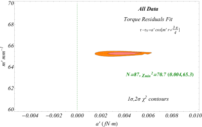
Figure 17: The $1\sigma$ and $2\sigma$ contours in the parametric space $(\alpha^{\prime},m^{\prime})$ for the oscillating parametrization (70). The quality of fit is significantly improved compared to the Newtonian ansatz. (from Ref. Perivolaropoulos (2017))

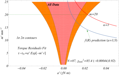
Figure 18: The $1\sigma$ and $2\sigma$ contours in the parametric space $(\alpha^{\prime},m^{\prime})$ for the Yukawa parametrization, (69). Despite the additional parameters the quality of fit is practically not improved compared to the Newtonian ansatz. (from Ref. Perivolaropoulos (2017))

The eighty seven residual datapoints superposed with the best fit Yukawa and the oscillating parametrizations are illustrated n Fig. 19 along with the best fit values of $\chi^{2}$.

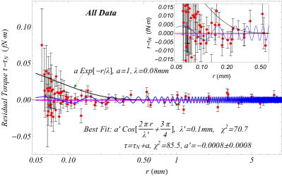
Figure 19: The residual data (torques) that it was considered in Ref. Perivolaropoulos (2017). The pink line denotes the best fit Yukawa parametrization, while the thin blue line describes the oscillating parametrization.

The statistical significance of the $\chi^{2}$ minimum ($\delta\chi^{2}\simeq-15$) corresponding to the best fit parameters $(\alpha^{\prime},m^{\prime})=(0.004fN\cdot m,65mm^{-1})$ of the oscillating parametrization is more than $3\sigma$ for a two-parameter parametrization. However, the existence of multiple minima in the parameter space $(\alpha^{\prime},m^{\prime})$ with similar depths reduces the statistical significance of this signal. The existence of such additional minima is demonstrated in Fig. 20 where we show $\chi^{2}(m^{\prime})$ where for each $m^{\prime}$ minimization with respect to $\alpha^{\prime}$ has been performed. For example the minima corresponding to $m^{\prime}\simeq 195mm^{-1}$ and $m^{\prime}\simeq 202mm^{-1}$ have comparable depths with the main minimum at $m^{\prime}\simeq 65mm^{-1}$ but they are effectively higher harmonics of this deepest minimum.

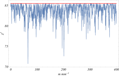
Figure 20: The value of the minimized $\chi^{2}$ as a function of the spatial frequency $m$. The red straight line is for $\delta\tau=0$ (from Ref. Perivolaropoulos (2017))

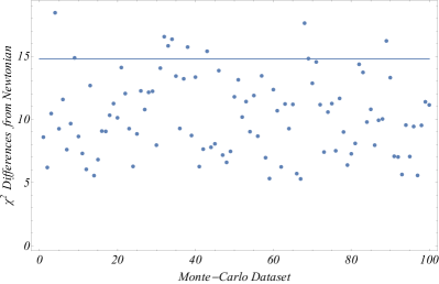
Figure 21: About $10\%$ of the Monte Carlo datasets created under the assumption of zero residuals (Newtonian model) have a $\delta\chi^{2}$ larger than the $\delta\chi^{2}$ of the real data when fitting the oscillating parametrization (70) for the torque residuals.

In order to estimate the significance of the deepest $\chi^{2}$ minimum at $m\simeq 65mm^{-1}$ Monte Carlo simulations were performed Perivolaropoulos (2017) (100 realizations) of the 87 data from the Washington experiment assuming a Gaussian distribution of the residuals around a Newtonian potential ($\delta\tau=0$) and standard deviation equal to the errorbars of the residuals. Using each Monte-Carlo realization $\chi^{2}(\alpha^{\prime},m^{\prime},\theta)$ was minimized for $m^{\prime}$ in the range $0-100mm^{-1}$ using the oscillating parametrization (70). The depth $\delta\chi^{2}\equiv\chi^{2}(\alpha^{\prime}=0)-\chi_{min}^{2}$ corresponding to each simulated Monte-Carlo dataset was then compared to the corresponding depth $\delta\chi^{2}\simeq 15$ of the real data. About $10\%$ of the simulated Newtonian data had a larger depth $\delta\chi^{2}$ than the real data (Fig. 21). Thus, the probability that the oscillating signal in the Washington experiment data is a statistical fluctuation is about $10\%$.

Therefore, there is an oscillation signal in the data whose origin could be either statistical, systematic or physical. In the later case, it is important to identify physical theories that are consistent with such an oscillating signal since as discussed above such a signal is not consistent with the simplest modified gravity theories as it is associated with instabilities. As shown in the next section however a class of theories involving infinite derivatives in the Lagrangian (nonlocal theories of gravity) naturally predict the existence of such oscillations on sub-mm scales.

III.4 Oscillating Newtonian Potential from Non-Local Gravity Theories

The Lagrangian of non-local gravity theories may be written as Biswas et al. (2012)

$$L_{IDG}=\frac{1}{8\pi G}\sqrt{-g}\left[R+\alpha\left(RF_{1}(\square)R+R^{\mu\nu}F_{2}(\square)R_{\mu\nu}+R^{\mu\nu\rho\sigma}F_{3}(\square)R_{\mu\nu\rho\sigma}\right)\right]$$ (72)

where

$$F_{i}(\square)=\sum_{n=0}^{\infty}f_{i,n}\left(\frac{\square}{m^{2}}\right)^{n}\quad\square=g^{\mu\nu}\nabla_{\mu}\nabla_{\nu}$$ (73)

Such a Lagrangian involving infinite higher derivative terms may offer the solution to some basic problems of GR, such as the behaviour of GR at small scales (GR predicts singularities at small scales). A related issue is the existence of unrenormalisable UV divergences in GR Goroff and Sagnotti (1986). These divergences can be alleviated if an Einstein-Hilbert action with higher derivative terms is considered Stelle (1978). These higher terms, however, are related with instabilities at the quantum level since the gravitational propagator imposed from these theories has a spin 2 component, which leads to an unhealthy classical vacuum theory (unstable). These extra problems can be resolved if we take infinite number of higher derivatives in the action, i.e. making the theory nonlocal, which modifies appropriately the gravitational propagator Biswas et al. (2012). These infinite derivatives are usually condensed in an exponential term for the avoidance of introducing new poles. Tomboulis (1997); Siegel (2003); Deser and Redlich (1986); Modesto (2012)

Thus nonlocal gravity theories provide the following advantages:

• They soften the UV divergences present at the quantum level along with the singularities of Big Bang and Black Holes. Biswas et al. (2012); Frolov (2008).

• They modify the Newtonian potential at the scale of nonlocality $m$, removing the divergences of the Newtonian potential at $r=0$, while in many cases they predict the existence decaying spatial oscillations of the gravitational potential on scales smaller than the nonlocality scale $m$. Edholm et al. (2016); Kehagias and Maggiore (2014); Frolov and Zelnikov (2016); Maggiore and Mancarella (2014)

• They are consistent with cosmological observations as they can provide a mechanism producing the observed accelerating expansion of the universe. Park and Dodelson (2013); Calcagni and Nardelli (2010); Barvinsky (2012); Dirian et al. (2016)

In the nonlocal theories the modified Newtonian potential is Edholm et al. (2016)

$$V_{\rm eff}(r)=-\frac{GM}{r}f(r,m)$$ (74)

where

$$f(r,m)=\frac{1}{\pi}\int_{-\infty}^{+\infty}dk\frac{sin(kr)e^{-\tau(k,m)}}{k}$$ (75)

Setting $\tau$ as

$$\tau=\frac{k^{2n}}{m^{2n}}$$ (76)

which is a typical form for $\tau$ and $n=1$, then Eq.(75) is rewritten as

$$f(r)=Erf(m\frac{r}{2})$$ (77)

which for $\bar{r}\equiv m\;r<<1$ takes a linear form and for $\bar{r}\gg 1$ it approaches unity. $f(r)$ is shown in Fig. 22, for two different values of $n$

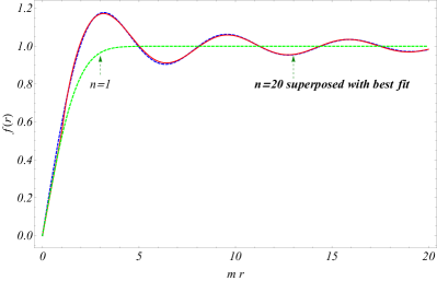
Figure 22: The plot of $f(r)$ for $n=1$ and $n=20$ denoted with dashed green and red line respectively along with the fit of (78),(79) (from Ref. Perivolaropoulos (2017))

For large $n$, $f(r)$ can be approximated very well by the following functions Perivolaropoulos (2017)

$$f(r) = \alpha_{1}\bar{r}\hskip 5.69046pt0<\bar{r}<1$$ (78)

$$f(r) = 1+\alpha_{2}\frac{\cos(\bar{r}+\theta)}{\bar{r}}\hskip 5.69046pt1<\bar{r}$$ (79)

where $\alpha_{1}=0.544$, $\alpha_{2}=0.572$, $\theta=0.885\pi$ (see also Ref. Edholm and Conroy (2017) for a similar parametrization).

Such models are interesting since not only they are free from UV divergences and singularities but the have a well-defined Newtonian limit. Therefore, this type of oscillating behavior may have been the origin of the oscillating signal in the data of the Washington experiment discussed in the previous sub-section.

IV Conclusions

In the present brief review, we discussed experimental and observational data on the smallest and the largest scales where gravity can be directly probed with current technology. We demonstrated that current data indicate the presence of hints of modified gravity in both the cosmological and the sub-millimeter scales. Concerning the cosmological scales, we showed that the best fit Planck15/$\Lambda$CDM $\sigma_{8}-\Omega_{m}$ parameter values are more than $3\sigma$ away from the corresponding best fit parameter values obtained using the latest RSD growth rate data ${\rm{\it f\sigma}}_{8}$, assuming a Planck15/$\Lambda$CDM background cosmology Nesseris et al. (2017). This tension has also been observed from various weak gravitational lensing analyses Joudaki et al. (2018); Abbott et al. (2017b).

The tension can be reduced either by reducing the value of $\Omega_{m}$ in the context of a $\Lambda$CDM cosmology or by allowing for an evolving Newton’s constant $G_{\rm eff}(z)$ leading to weaker gravity at $z\simeq 1$. In particular we showed that a Planck15/$\Lambda$CDM $H(z)$ cosmological background with a well motivated form of $G_{\rm eff}(z)=1+g_{a}\left(\frac{z}{1+z}\right)^{n}-g_{a}\left(\frac{z}{1+z}\right)^{2n}$, which is a decreasing function of $z$ (for $g_{a}<0$), can be significantly more consistent with the full dataset of ${\rm{\it f\sigma}}_{8}$ from Ref. Kazantzidis and Perivolaropoulos (2018). This type of evolution cannot be reproduced in scalar-tensor theories with a $\Lambda$CDM background, since it leads to negative kinetic term of the scalar field $\phi(z)$. One possible way to reproduce a decreasing $G_{\rm eff}(z)$ in scalar-tensor theories would be to assume for a wCDM expansion background with $w>-1$. For example we demonstrated that for a wCDM background, $G_{\rm eff}(z)$ can be a decreasing function of $z$ in the context of scalar-tensor theories.

Finally on sub-mm scales higher derivative gravity models generically predict sub-mm spatial oscillations of the gravitational potential. Hints for such oscillations have been demonstrated to exist in the Washington torsion-balance experiment.

Thus we have demonstrated the existence of hints for deviations from GR on both the largest scales where a $G_{\rm eff}(z<1)<G_{N}$ is favored and on the smallest probed scales (sub-mm) where an oscillating $G_{\rm eff}(r)$ is favored. It is therefore important to clarify if these hints are due to systematic or statistical effects or they constitute early manifestation for new physics. This clarification may be achieved by considering new larger datasets focusing on the redshifts/scales where these hints appear $(z\simeq 0.3\text{ and }r\simeq 80\mu m).$

Appendix A Data Used in the Analysis

Table 5: The ${\rm{\it f\sigma}}_{8}$ data compilation from Ref. Kazantzidis and Perivolaropoulos (2018)

Index	Dataset	$z$	$f\sigma_{8}(z)$	Refs.	Year	Fiducial Cosmology
1	SDSS-LRG	$0.35$	$0.440\pm 0.050$	Song and Percival (2009)	30 October 2006	$(\Omega_{m},\Omega_{K},\sigma_{8}$)$=(0.25,0,0.756)$Tegmark et al. (2006)
2	VVDS	$0.77$	$0.490\pm 0.18$	Song and Percival (2009)	6 October 2009	$(\Omega_{m},\Omega_{K},\sigma_{8})=(0.25,0,0.78)$
3	2dFGRS	$0.17$	$0.510\pm 0.060$	Song and Percival (2009)	6 October 2009	$(\Omega_{m},\Omega_{K})=(0.3,0,0.9)$
4	2MRS	0.02	$0.314\pm 0.048$	Davis et al. (2011), Hudson and Turnbull (2012)	13 Novemver 2010	$(\Omega_{m},\Omega_{K},\sigma_{8})=(0.266,0,0.65)$
5	SnIa+IRAS	0.02	$0.398\pm 0.065$	Turnbull et al. (2012), Hudson and Turnbull (2012)	20 October 2011	$(\Omega_{m},\Omega_{K},\sigma_{8})=(0.3,0,0.814)$
6	SDSS-LRG-200	$0.25$	$0.3512\pm 0.0583$	Samushia et al. (2012)	9 December 2011	$(\Omega_{m},\Omega_{K},\sigma_{8})=(0.276,0,0.8)$
7	SDSS-LRG-200	$0.37$	$0.4602\pm 0.0378$	Samushia et al. (2012)	9 December 2011
8	SDSS-LRG-60	$0.25$	$0.3665\pm 0.0601$	Samushia et al. (2012)	9 December 2011	$(\Omega_{m},\Omega_{K},\sigma_{8})=(0.276,0,0.8)$
9	SDSS-LRG-60	$0.37$	$0.4031\pm 0.0586$	Samushia et al. (2012)	9 December 2011
10	WiggleZ	$0.44$	$0.413\pm 0.080$	Blake et al. (2012)	12 June 2012	$(\Omega_{m},h,\sigma_{8})=(0.27,0.71,0.8)$
11	WiggleZ	$0.60$	$0.390\pm 0.063$	Blake et al. (2012)	12 June 2012
12	WiggleZ	$0.73$	$0.437\pm 0.072$	Blake et al. (2012)	12 June 2012
13	6dFGS	$0.067$	$0.423\pm 0.055$	Beutler et al. (2012)	4 July 2012	$(\Omega_{m},\Omega_{K},\sigma_{8})=(0.27,0,0.76)$
14	SDSS-BOSS	$0.30$	$0.407\pm 0.055$	Tojeiro et al. (2012)	11 August 2012	$(\Omega_{m},\Omega_{K},\sigma_{8})=(0.25,0,0.804)$
15	SDSS-BOSS	$0.40$	$0.419\pm 0.041$	Tojeiro et al. (2012)	11 August 2012
16	SDSS-BOSS	$0.50$	$0.427\pm 0.043$	Tojeiro et al. (2012)	11 August 2012
17	SDSS-BOSS	$0.60$	$0.433\pm 0.067$	Tojeiro et al. (2012)	11 August 2012
18	Vipers	$0.80$	$0.470\pm 0.080$	de la Torre et al. (2013)	9 July 2013	$(\Omega_{m},\Omega_{K},\sigma_{8})=(0.25,0,0.82)$
19	SDSS-DR7-LRG	$0.35$	$0.429\pm 0.089$	Chuang and Wang (2013)	8 August 2013	$(\Omega_{m},\Omega_{K},\sigma_{8}$)$=(0.25,0,0.809)$Komatsu et al. (2011)
20	GAMA	$0.18$	$0.360\pm 0.090$	Blake et al. (2013)	22 September 2013	$(\Omega_{m},\Omega_{K},\sigma_{8})=(0.27,0,0.8)$
21	GAMA	$0.38$	$0.440\pm 0.060$	Blake et al. (2013)	22 September 2013
22	BOSS-LOWZ	$0.32$	$0.384\pm 0.095$	Sanchez et al. (2014)	17 December 2013	$(\Omega_{m},\Omega_{K},\sigma_{8})=(0.274,0,0.8)$
23	SDSS DR10 and DR11	$0.32$	$0.48\pm 0.10$	Sanchez et al. (2014)	17 December 2013	$(\Omega_{m},\Omega_{K},\sigma_{8}$)$=(0.274,0,0.8)$Anderson et al. (2014)
24	SDSS DR10 and DR11	$0.57$	$0.417\pm 0.045$	Sanchez et al. (2014)	17 December 2013
25	SDSS-MGS	$0.15$	$0.490\pm 0.145$	Howlett et al. (2015)	30 January 2015	$(\Omega_{m},h,\sigma_{8})=(0.31,0.67,0.83)$
26	SDSS-veloc	$0.10$	$0.370\pm 0.130$	Feix et al. (2015)	16 June 2015	$(\Omega_{m},\Omega_{K},\sigma_{8}$)$=(0.3,0,0.89)$Tegmark et al. (2004)
27	FastSound	$1.40$	$0.482\pm 0.116$	Okumura et al. (2016)	25 November 2015	$(\Omega_{m},\Omega_{K},\sigma_{8}$)$=(0.27,0,0.82)$Hinshaw et al. (2013)
28	SDSS-CMASS	$0.59$	$0.488\pm 0.060$	Chuang et al. (2016)	8 July 2016	$\ \ (\Omega_{m},h,\sigma_{8})=(0.307115,0.6777,0.8288)$
29	BOSS DR12	$0.38$	$0.497\pm 0.045$	Alam et al. (2017)	11 July 2016	$(\Omega_{m},\Omega_{K},\sigma_{8})=(0.31,0,0.8)$
30	BOSS DR12	$0.51$	$0.458\pm 0.038$	Alam et al. (2017)	11 July 2016
31	BOSS DR12	$0.61$	$0.436\pm 0.034$	Alam et al. (2017)	11 July 2016
32	BOSS DR12	$0.38$	$0.477\pm 0.051$	Beutler et al. (2017)	11 July 2016	$(\Omega_{m},h,\sigma_{8})=(0.31,0.676,0.8)$
33	BOSS DR12	$0.51$	$0.453\pm 0.050$	Beutler et al. (2017)	11 July 2016
34	BOSS DR12	$0.61$	$0.410\pm 0.044$	Beutler et al. (2017)	11 July 2016
35	Vipers v7	$0.76$	$0.440\pm 0.040$	Wilson (2016)	26 October 2016	$(\Omega_{m},\sigma_{8})=(0.308,0.8149)$
36	Vipers v7	$1.05$	$0.280\pm 0.080$	Wilson (2016)	26 October 2016
37	BOSS LOWZ	$0.32$	$0.427\pm 0.056$	Gil-Marín et al. (2017)	26 October 2016	$(\Omega_{m},\Omega_{K},\sigma_{8})=(0.31,0,0.8475)$
38	BOSS CMASS	$0.57$	$0.426\pm 0.029$	Gil-Marín et al. (2017)	26 October 2016
39	Vipers	$0.727$	$0.296\pm 0.0765$	Hawken et al. (2017)	21 November 2016	$(\Omega_{m},\Omega_{K},\sigma_{8})=(0.31,0,0.7)$
40	6dFGS+SnIa	$0.02$	$0.428\pm 0.0465$	Huterer et al. (2017)	29 November 2016	$(\Omega_{m},h,\sigma_{8})=(0.3,0.683,0.8)$
41	Vipers	$0.6$	$0.48\pm 0.12$	de la Torre et al. (2017)	16 December 2016	$(\Omega_{m},\Omega_{b},n_{s},\sigma_{8}$)= $(0.3,0.045,0.96,0.831)$Ade et al. (2016)
42	Vipers	$0.86$	$0.48\pm 0.10$	de la Torre et al. (2017)	16 December 2016
43	Vipers PDR-2	$0.60$	$0.550\pm 0.120$	Pezzotta et al. (2017)	16 December 2016	$(\Omega_{m},\Omega_{b},\sigma_{8})=(0.3,0.045,0.823)$
44	Vipers PDR-2	$0.86$	$0.400\pm 0.110$	Pezzotta et al. (2017)	16 December 2016
45	SDSS DR13	$0.1$	$0.48\pm 0.16$	Feix et al. (2017)	22 December 2016	$(\Omega_{m},\sigma_{8}$)$=(0.25,0.89)$Tegmark et al. (2004)
46	2MTF	0.001	$0.505\pm 0.085$	Howlett et al. (2017)	16 June 2017	$(\Omega_{m},\sigma_{8})=(0.3121,0.815)$
47	Vipers PDR-2	$0.85$	$0.45\pm 0.11$	Mohammad et al. (2017)	31 July 2017	$(\Omega_{b},\Omega_{m},h)=(0.045,0.30,0.8)$
48	BOSS DR12	$0.31$	$0.469\pm 0.098$	Wang et al. (2017)	15 September 2017	$(\Omega_{m},h,\sigma_{8})=(0.307,0.6777,0.8288)$
49	BOSS DR12	$0.36$	$0.474\pm 0.097$	Wang et al. (2017)	15 September 2017
50	BOSS DR12	$0.40$	$0.473\pm 0.086$	Wang et al. (2017)	15 September 2017
51	BOSS DR12	$0.44$	$0.481\pm 0.076$	Wang et al. (2017)	15 September 2017
52	BOSS DR12	$0.48$	$0.482\pm 0.067$	Wang et al. (2017)	15 September 2017
53	BOSS DR12	$0.52$	$0.488\pm 0.065$	Wang et al. (2017)	15 September 2017
54	BOSS DR12	$0.56$	$0.482\pm 0.067$	Wang et al. (2017)	15 September 2017
55	BOSS DR12	$0.59$	$0.481\pm 0.066$	Wang et al. (2017)	15 September 2017
56	BOSS DR12	$0.64$	$0.486\pm 0.070$	Wang et al. (2017)	15 September 2017
57	SDSS DR7	$0.1$	$0.376\pm 0.038$	Shi et al. (2017)	12 December 2017	$(\Omega_{m},\Omega_{b},\sigma_{8})=(0.282,0.046,0.817)$
58	SDSS-IV	$1.52$	$0.420\pm 0.076$	Gil-Marín et al. (2018)	8 January 2018	$(\Omega_{m},\Omega_{b}h^{2},\sigma_{8})=(0.26479,0.02258,0.8)$
59	SDSS-IV	$1.52$	$0.396\pm 0.079$	Hou et al. (2018)	8 January 2018	$(\Omega_{m},\Omega_{b}h^{2},\sigma_{8})=(0.31,0.022,0.8225)$
60	SDSS-IV	$0.978$	$0.379\pm 0.176$	Zhao et al. (2018)	9 January 2018	$(\Omega_{m},\sigma_{8})=(0.31,0.8)$
61	SDSS-IV	$1.23$	$0.385\pm 0.099$	Zhao et al. (2018)	9 January 2018
62	SDSS-IV	$1.526$	$0.342\pm 0.070$	Zhao et al. (2018)	9 January 2018
63	SDSS-IV	$1.944$	$0.364\pm 0.106$	Zhao et al. (2018)	9 January 2018

Table 6: A compilation of robust and independent $f\sigma_{8}(z)$ measurements from different surveys. In the columns we show in ascending order with respect to redshift, the name and year of the survey that made the measurement, the redshift and value of $f\sigma_{8}(z)$ and the corresponding reference and fiducial cosmology

Index	Dataset	$z$	$f\sigma_{8}(z)$	Refs.	Year	Fiducial Cosmology
1	6dFGS+SnIa	$0.02$	$0.428\pm 0.0465$	Huterer et al. (2017)	2016	$(\Omega_{m},h,\sigma_{8})=(0.3,0.683,0.8)$
2	SnIa+IRAS	0.02	$0.398\pm 0.065$	Turnbull et al. (2012),Hudson and Turnbull (2012)	2011	$(\Omega_{m},\Omega_{K})=(0.3,0)$
3	2MASS	0.02	$0.314\pm 0.048$	Davis et al. (2011),Hudson and Turnbull (2012)	2010	$(\Omega_{m},\Omega_{K})=(0.266,0)$
4	SDSS-veloc	$0.10$	$0.370\pm 0.130$	Feix et al. (2015)	2015	$(\Omega_{m},\Omega_{K})=(0.3,0)$
5	SDSS-MGS	$0.15$	$0.490\pm 0.145$	Howlett et al. (2015)	2014	$(\Omega_{m},h,\sigma_{8})=(0.31,0.67,0.83)$
6	2dFGRS	$0.17$	$0.510\pm 0.060$	Song and Percival (2009)	2009	$(\Omega_{m},\Omega_{K})=(0.3,0)$
7	GAMA	$0.18$	$0.360\pm 0.090$	Blake et al. (2013)	2013	$(\Omega_{m},\Omega_{K})=(0.27,0)$
8	GAMA	$0.38$	$0.440\pm 0.060$	Blake et al. (2013)	2013
9	SDSS-LRG-200	$0.25$	$0.3512\pm 0.0583$	Samushia et al. (2012)	2011	$(\Omega_{m},\Omega_{K})=(0.25,0)$
10	SDSS-LRG-200	$0.37$	$0.4602\pm 0.0378$	Samushia et al. (2012)	2011
11	BOSS-LOWZ	$0.32$	$0.384\pm 0.095$	Sanchez et al. (2014)	2013	$(\Omega_{m},\Omega_{K})=(0.274,0)$
12	SDSS-CMASS	$0.59$	$0.488\pm 0.060$	Chuang et al. (2016)	2013	$\ \ (\Omega_{m},h,\sigma_{8})=(0.307115,0.6777,0.8288)$
13	WiggleZ	$0.44$	$0.413\pm 0.080$	Blake et al. (2012)	2012	$(\Omega_{m},h)=(0.27,0.71)$
14	WiggleZ	$0.60$	$0.390\pm 0.063$	Blake et al. (2012)	2012
15	WiggleZ	$0.73$	$0.437\pm 0.072$	Blake et al. (2012)	2012
16	Vipers PDR-2	$0.60$	$0.550\pm 0.120$	Pezzotta et al. (2017)	2016	$(\Omega_{m},\Omega_{b})=(0.3,0.045)$
17	Vipers PDR-2	$0.86$	$0.400\pm 0.110$	Pezzotta et al. (2017)	2016
18	FastSound	$1.40$	$0.482\pm 0.116$	Okumura et al. (2016)	2015	$(\Omega_{m},\Omega_{K})=(0.270,0)$

References

- Kapner et al. (2007a) D. J. Kapner, T. S. Cook, E. G. Adelberger, J. H. Gundlach, Blayne R. Heckel, C. D. Hoyle, and H. E. Swanson, “Tests of the gravitational inverse-square law below the dark-energy length scale,” Phys. Rev. Lett. 98, 021101 (2007a), arXiv:hep-ph/0611184 [hep-ph] .
- Will (2014) Clifford M. Will, “The Confrontation between General Relativity and Experiment,” Living Rev. Rel. 17, 4 (2014), arXiv:1403.7377 [gr-qc] .
- Anderson et al. (2002) John D. Anderson, Philip A. Laing, Eunice L. Lau, Michael Martin Nieto, and Slava G. Turyshev, “The search for a standard explanation of the Pioneer anomaly,” Mod. Phys. Lett. A17, 875–886 (2002), arXiv:gr-qc/0107022 [gr-qc] .
- Sokolov (2016) V. V. Sokolov, “On the observed mass distribution of compact stellar remnants in close binary systems and possible interpretations proposed for the time being,” in Quark Phase Transition in Compact Objects and Multimessenger Astronomy: Neutrino Signals, Supernovae and Gamma-Ray Bursts, edited by V. V. Sokolov, V. V. Vlasyuk, and V. B. Petkov (2016) pp. 121–132.
- Jungman et al. (1996) Gerard Jungman, Marc Kamionkowski, and Kim Griest, “Supersymmetric dark matter,” Phys. Rept. 267, 195–373 (1996), arXiv:hep-ph/9506380 [hep-ph] .
- Bekenstein (2004) Jacob D. Bekenstein, “Relativistic gravitation theory for the MOND paradigm,” Phys. Rev. D70, 083509 (2004), [Erratum: Phys. Rev.D71,069901(2005)], arXiv:astro-ph/0403694 [astro-ph] .
- Abbott et al. (2017a) B. P. Abbott et al. (LIGO Scientific, Virgo), “GW170817: Observation of Gravitational Waves from a Binary Neutron Star Inspiral,” Phys. Rev. Lett. 119, 161101 (2017a), arXiv:1710.05832 [gr-qc] .
- Boran et al. (2018) S. Boran, S. Desai, E. O. Kahya, and R. P. Woodard, “GW170817 Falsifies Dark Matter Emulators,” Phys. Rev. D97, 041501 (2018), arXiv:1710.06168 [astro-ph.HE] .
- Green et al. (2018) M. A. Green, J. W. Moffat, and V. T. Toth, “Modified Gravity (MOG), the speed of gravitational radiation and the event GW170817/GRB170817A,” Phys. Lett. B780, 300–302 (2018), arXiv:1710.11177 [gr-qc] .
- Moffat (2006) J. W. Moffat, “Scalar-tensor-vector gravity theory,” JCAP 0603, 004 (2006), arXiv:gr-qc/0506021 [gr-qc] .
- Milgrom (1983a) M. Milgrom, “A Modification of the Newtonian dynamics as a possible alternative to the hidden mass hypothesis,” Astrophys. J. 270, 365–370 (1983a).
- Milgrom (1983b) M. Milgrom, “A Modification of the Newtonian dynamics: Implications for galaxies,” Astrophys. J. 270, 371–383 (1983b).
- Milgrom (1983c) M. Milgrom, “A modification of the Newtonian dynamics: implications for galaxy systems,” Astrophys. J. 270, 384–389 (1983c).
- Christodoulou and Kazanas (2018) Dimitris M. Christodoulou and Demosthenes Kazanas, “Interposing a Varying Gravitational Constant Between Modified Newtonian Dynamics and Weak Weyl Gravity,” Mon. Not. Roy. Astron. Soc. 479, L143–L147 (2018), arXiv:1806.09778 [gr-qc] .
- Christodoulou and Kazanas (2019a) Dimitris M. Christodoulou and Demosthenes Kazanas, “Gravitational potential and non-relativistic Lagrangian in modified gravity with varying G,” Mon. Not. Roy. Astron. Soc. 483, L85–L87 (2019a), arXiv:1811.08920 [astro-ph.GA] .
- Christodoulou and Kazanas (2019b) Dimitris M. Christodoulou and Demosthenes Kazanas, “Gauss’s law and the source for Poisson’s equation in modified gravity with Varying G,” Mon. Not. Roy. Astron. Soc. 484, 1421–1425 (2019b), arXiv:1901.02589 [astro-ph.GA] .
- Christodoulou and Kazanas (2019c) Dimitris M. Christodoulou and Demosthenes Kazanas, “Universal expansion with spatially varying ,” (2019c), 10.1093/mnrasl/slz074, arXiv:1905.04296 [gr-qc] .
- Murata and Tanaka (2015) Jiro Murata and Saki Tanaka, “A review of short-range gravity experiments in the LHC era,” Class. Quant. Grav. 32, 033001 (2015), arXiv:1408.3588 [hep-ex] .
- Nesseris et al. (2017) Savvas Nesseris, George Pantazis, and Leandros Perivolaropoulos, “Tension and constraints on modified gravity parametrizations of from growth rate and Planck data,” Phys. Rev. D96, 023542 (2017), arXiv:1703.10538 [astro-ph.CO] .
- Macaulay et al. (2013) Edward Macaulay, Ingunn Kathrine Wehus, and Hans Kristian Eriksen, “Lower Growth Rate from Recent Redshift Space Distortion Measurements than Expected from Planck,” Phys. Rev. Lett. 111, 161301 (2013), arXiv:1303.6583 [astro-ph.CO] .
- Tsujikawa (2015) Shinji Tsujikawa, “Possibility of realizing weak gravity in redshift space distortion measurements,” Phys. Rev. D92, 044029 (2015), arXiv:1505.02459 [astro-ph.CO] .
- Johnson et al. (2016) Andrew Johnson, Chris Blake, Jason Dossett, Jun Koda, David Parkinson, and Shahab Joudaki, “Searching for Modified Gravity: Scale and Redshift Dependent Constraints from Galaxy Peculiar Velocities,” Mon. Not. Roy. Astron. Soc. 458, 2725–2744 (2016), arXiv:1504.06885 [astro-ph.CO] .
- Basilakos and Nesseris (2017) Spyros Basilakos and Savvas Nesseris, “Conjoined constraints on modified gravity from the expansion history and cosmic growth,” Phys. Rev. D96, 063517 (2017), arXiv:1705.08797 [astro-ph.CO] .
- Kazantzidis and Perivolaropoulos (2018) Lavrentios Kazantzidis and Leandros Perivolaropoulos, “Evolution of the tension with the Planck15/CDM determination and implications for modified gravity theories,” Phys. Rev. D97, 103503 (2018), arXiv:1803.01337 [astro-ph.CO] .
- Joudaki et al. (2018) Shahab Joudaki et al., “KiDS-450 + 2dFLenS: Cosmological parameter constraints from weak gravitational lensing tomography and overlapping redshift-space galaxy clustering,” Mon. Not. Roy. Astron. Soc. 474, 4894–4924 (2018), arXiv:1707.06627 [astro-ph.CO] .
- Hildebrandt et al. (2017) H. Hildebrandt et al., “KiDS-450: Cosmological parameter constraints from tomographic weak gravitational lensing,” Mon. Not. Roy. Astron. Soc. 465, 1454 (2017), arXiv:1606.05338 [astro-ph.CO] .
- Troxel et al. (2018) M. A. Troxel et al. (DES), “Dark Energy Survey Year 1 results: Cosmological constraints from cosmic shear,” Phys. Rev. D98, 043528 (2018), arXiv:1708.01538 [astro-ph.CO] .
- Köhlinger et al. (2017) F. Köhlinger et al., “KiDS-450: The tomographic weak lensing power spectrum and constraints on cosmological parameters,” Mon. Not. Roy. Astron. Soc. 471, 4412–4435 (2017), arXiv:1706.02892 [astro-ph.CO] .
- Lamoreaux (1997) S. K. Lamoreaux, “Demonstration of the Casimir force in the 0.6 to 6 micrometers range,” Phys. Rev. Lett. 78, 5–8 (1997), [Erratum: Phys. Rev. Lett.81,5475(1998)].
- Chiaverini et al. (2003) J. Chiaverini, S. J. Smullin, A. A. Geraci, D. M. Weld, and A. Kapitulnik, “New experimental constraints on nonNewtonian forces below 100 microns,” Phys. Rev. Lett. 90, 151101 (2003), arXiv:hep-ph/0209325 [hep-ph] .
- Smullin et al. (2005) S. J. Smullin, A. A. Geraci, D. M. Weld, J. Chiaverini, Susan P. Holmes, and A. Kapitulnik, “New constraints on Yukawa-type deviations from Newtonian gravity at 20 microns,” Phys. Rev. D72, 122001 (2005), [Erratum: Phys. Rev.D72,129901(2005)], arXiv:hep-ph/0508204 [hep-ph] .
- Geraci et al. (2008) Andrew A. Geraci, Sylvia J. Smullin, David M. Weld, John Chiaverini, and Aharon Kapitulnik, “Improved constraints on non-Newtonian forces at 10 microns,” Phys. Rev. D78, 022002 (2008), arXiv:0802.2350 [hep-ex] .
- Long et al. (2002) Joshua C. Long, Hilton W. Chan, Allison B. Churnside, Eric A. Gulbis, Michael C. M. Varney, and John C. Price, “Upper limits to submillimeter-range forces from extra space-time dimensions,” (2002), 10.1038/nature01432, [Nature421,922(2003)], arXiv:hep-ph/0210004 [hep-ph] .
- Mitrofanov and Ponomareva (1988) V. P. Mitrofanov and O. I. Ponomareva, Sov. Phys. JETP 87, 1963–1966 (1988).
- Hoyle et al. (2004a) C. D. Hoyle, D. J. Kapner, Blayne R. Heckel, E. G. Adelberger, J. H. Gundlach, U. Schmidt, and H. E. Swanson, “Sub-millimeter tests of the gravitational inverse-square law,” Phys. Rev. D70, 042004 (2004a), arXiv:hep-ph/0405262 [hep-ph] .
- Hoyle et al. (2001) C. D. Hoyle, U. Schmidt, Blayne R. Heckel, E. G. Adelberger, J. H. Gundlach, D. J. Kapner, and H. E. Swanson, “Submillimeter tests of the gravitational inverse square law: a search for ’large’ extra dimensions,” Phys. Rev. Lett. 86, 1418–1421 (2001), arXiv:hep-ph/0011014 [hep-ph] .
- Kapner et al. (2007b) D. J. Kapner, T. S. Cook, E. G. Adelberger, J. H. Gundlach, Blayne R. Heckel, C. D. Hoyle, and H. E. Swanson, “Tests of the gravitational inverse-square law below the dark-energy length scale,” Phys. Rev. Lett. 98, 021101 (2007b), arXiv:hep-ph/0611184 [hep-ph] .
- Tu et al. (2007) Liang-Cheng Tu, Sheng-Guo Guan, Jun Luo, Cheng-Gang Shao, and Lin-Xia Liu, “Null Test of Newtonian Inverse-Square Law at Submillimeter Range with a Dual-Modulation Torsion Pendulum,” Phys. Rev. Lett. 98, 201101 (2007).
- Yang et al. (2012) Shan-Qing Yang, Bi-Fu Zhan, Qing-Lan Wang, Cheng-Gang Shao, Liang-Cheng Tu, Wen-Hai Tan, and Jun Luo, “Test of the Gravitational Inverse Square Law at Millimeter Ranges,” Phys. Rev. Lett. 108, 081101 (2012).
- et. al. (2014) Murata J. et. al., Hyperfine Interaction 255, 193–196 (2014).
- Hoskins et al. (1985) J. K. Hoskins, R. D. Newman, R. Spero, and J. Schultz, “Experimental tests of the gravitational inverse square law for mass separations from 2-cm to 105-cm,” Phys. Rev. D32, 3084–3095 (1985).
- Spero et al. (1980) R. Spero, J. K. Hoskins, R. Newman, J. Pellam, and J. Schultz, “Test of the Gravitational Inverse-Square Law at Laboratory Distances,” Phys. Rev. Lett. 44, 1645–1648 (1980).
- Milyukov (1985) V. K. Milyukov, Sov. Phys. JETP 61, 187–191 (1985).
- Panov and Frontov (1979) V. I. Panov and V. N. Frontov, Sov. Phys. JETP 50, 852–856 (1979).
- Moody and Paik (1993) M. V. Moody and H. J. Paik, “Gauss’s law test of gravity at short range,” Phys. Rev. Lett. 70, 1195–1198 (1993).
- H. et al. (1980) Hirakawa H., Tsubono K., and Oide K., Nature 283, 184–185 (1980).
- Y. et al. (1982) Ogawa Y., Tsubono K., and Hirakawa H., Phys. Rev. D 32, 342–346 (1982).
- K. and H. (1985) Kuroda K. and Hirakawa H., Phys. Rev. D 32, 342–346 (1985).
- N. et al. (1987) Mio N., Tsubono K., and Hirakawa H., Phys. Rev. D 36, 2321–2326 (1987).
- Brax et al. (2019) Philippe Brax, Patrick Valageas, and Pierre Vanhove, “New Bounds on Dark Energy Induced Fifth Forces,” Phys. Rev. D99, 064010 (2019), arXiv:1902.07555 [astro-ph.CO] .
- Perivolaropoulos (2010) L. Perivolaropoulos, “PPN Parameter gamma and Solar System Constraints of Massive Brans-Dicke Theories,” Phys. Rev. D81, 047501 (2010), arXiv:0911.3401 [gr-qc] .
- Hohmann et al. (2013) Manuel Hohmann, Laur Jarv, Piret Kuusk, and Erik Randla, “Post-Newtonian parameters and of scalar-tensor gravity with a general potential,” Phys. Rev. D88, 084054 (2013), [Erratum: Phys. Rev.D89,no.6,069901(2014)], arXiv:1309.0031 [gr-qc] .
- Järv et al. (2015) Laur Järv, Piret Kuusk, Margus Saal, and Ott Vilson, “Invariant quantities in the scalar-tensor theories of gravitation,” Phys. Rev. D91, 024041 (2015), arXiv:1411.1947 [gr-qc] .
- Esposito-Farese and Polarski (2001) Gilles Esposito-Farese and D. Polarski, “Scalar tensor gravity in an accelerating universe,” Phys. Rev. D63, 063504 (2001), arXiv:gr-qc/0009034 [gr-qc] .
- Gannouji et al. (2006) Radouane Gannouji, David Polarski, Andre Ranquet, and Alexei A. Starobinsky, “Scalar-Tensor Models of Normal and Phantom Dark Energy,” JCAP 0609, 016 (2006), arXiv:astro-ph/0606287 [astro-ph] .
- Faraoni (2004) Valerio Faraoni, Cosmology in scalar tensor gravity, Vol. 139 (2004).
- Chiba (2003a) Takeshi Chiba, “1/R gravity and scalar - tensor gravity,” Phys. Lett. B575, 1–3 (2003a), arXiv:astro-ph/0307338 [astro-ph] .
- Berry and Gair (2011) Christopher P. L. Berry and Jonathan R. Gair, “Linearized f(R) Gravity: Gravitational Radiation and Solar System Tests,” Phys. Rev. D83, 104022 (2011), [Erratum: Phys. Rev.D85,089906(2012)], arXiv:1104.0819 [gr-qc] .
- Capozziello et al. (2009) S. Capozziello, A. Stabile, and A. Troisi, “A General solution in the Newtonian limit of f(R)- gravity,” Mod. Phys. Lett. A24, 659–665 (2009), arXiv:0901.0448 [gr-qc] .
- Schellstede (2016) Gerold Oltman Schellstede, “On the Newtonian limit of metric f(R) gravity,” Gen. Rel. Grav. 48, 118 (2016).
- Perivolaropoulos (2003) L. Perivolaropoulos, “Equation of state of oscillating Brans-Dicke scalar and extra dimensions,” Phys. Rev. D67, 123516 (2003), arXiv:hep-ph/0301237 [hep-ph] .
- Perivolaropoulos (2017) Leandros Perivolaropoulos, “Submillimeter spatial oscillations of Newton’s constant: Theoretical models and laboratory tests,” Phys. Rev. D95, 084050 (2017), arXiv:1611.07293 [gr-qc] .
- Perivolaropoulos and Sourdis (2002) L. Perivolaropoulos and C. Sourdis, “Cosmological effects of radion oscillations,” Phys. Rev. D66, 084018 (2002), arXiv:hep-ph/0204155 [hep-ph] .
- Donini and Marimón (2016) A. Donini and S. G. Marimón, “Micro-orbits in a many-brane model and deviations from Newton’s law,” Eur. Phys. J. C76, 696 (2016), arXiv:1609.05654 [hep-ph] .
- Benichou and Estes (2012) Raphael Benichou and John Estes, “The Fate of Newton’s Law in Brane-World Scenarios,” Phys. Lett. B712, 456–459 (2012), arXiv:1112.0565 [hep-th] .
- Bronnikov et al. (2006) K. A. Bronnikov, S. A. Kononogov, and V. N. Melnikov, “Brane world corrections to Newton’s law,” Gen. Rel. Grav. 38, 1215–1232 (2006), arXiv:gr-qc/0601114 [gr-qc] .
- Nojiri and Odintsov (2002) Shin’ichi Nojiri and Sergei D. Odintsov, “Newton potential in deSitter brane world,” Phys. Lett. B548, 215–223 (2002), arXiv:hep-th/0209066 [hep-th] .
- Faraoni (2006a) Valerio Faraoni, “Matter instability in modified gravity,” Phys. Rev. D74, 104017 (2006a), arXiv:astro-ph/0610734 [astro-ph] .
- Dolgov and Kawasaki (2003) A. D. Dolgov and Masahiro Kawasaki, “Can modified gravity explain accelerated cosmic expansion?” Phys. Lett. B573, 1–4 (2003), arXiv:astro-ph/0307285 [astro-ph] .
- Edholm et al. (2016) James Edholm, Alexey S. Koshelev, and Anupam Mazumdar, “Behavior of the Newtonian potential for ghost-free gravity and singularity-free gravity,” Phys. Rev. D94, 104033 (2016), arXiv:1604.01989 [gr-qc] .
- Kehagias and Maggiore (2014) Alex Kehagias and Michele Maggiore, “Spherically symmetric static solutions in a nonlocal infrared modification of General Relativity,” JHEP 08, 029 (2014), arXiv:1401.8289 [hep-th] .
- Frolov and Zelnikov (2016) Valeri P. Frolov and Andrei Zelnikov, “Head-on collision of ultrarelativistic particles in ghost-free theories of gravity,” Phys. Rev. D93, 064048 (2016), arXiv:1509.03336 [hep-th] .
- Tomboulis (1997) E. T. Tomboulis, “Superrenormalizable gauge and gravitational theories,” (1997), arXiv:hep-th/9702146 [hep-th] .
- Siegel (2003) W. Siegel, “Stringy gravity at short distances,” (2003), arXiv:hep-th/0309093 [hep-th] .
- Biswas et al. (2014) Tirthabir Biswas, Aindriú Conroy, Alexey S. Koshelev, and Anupam Mazumdar, “Generalized ghost-free quadratic curvature gravity,” Class. Quant. Grav. 31, 015022 (2014), [Erratum: Class. Quant. Grav.31,159501(2014)], arXiv:1308.2319 [hep-th] .
- Alam et al. (2017) Shadab Alam et al. (BOSS), “The clustering of galaxies in the completed SDSS-III Baryon Oscillation Spectroscopic Survey: cosmological analysis of the DR12 galaxy sample,” Mon. Not. Roy. Astron. Soc. 470, 2617–2652 (2017), arXiv:1607.03155 [astro-ph.CO] .
- Amon et al. (2017) A. Amon et al., “KiDS+2dFLenS+GAMA: Testing the cosmological model with the statistic,” (2017), 10.1093/mnras/sty1624, arXiv:1711.10999 [astro-ph.CO] .
- Abbott et al. (2018) T. M. C. Abbott et al. (DES), “The Dark Energy Survey Data Release 1,” (2018), arXiv:1801.03181 [astro-ph.IM] .
- Ade et al. (2016) P. A. R. Ade et al. (Planck), “Planck 2015 results. XIII. Cosmological parameters,” Astron. Astrophys. 594, A13 (2016), arXiv:1502.01589 [astro-ph.CO] .
- Abbott et al. (2017b) T. M. C. Abbott et al. (DES), “Dark Energy Survey Year 1 Results: Cosmological Constraints from Galaxy Clustering and Weak Lensing,” (2017b), arXiv:1708.01530 [astro-ph.CO] .
- Blake et al. (2012) C. Blake, S. Brough, M. Colless, C. Contreras, W. Couch, S. Croom, D. Croton, T. M. Davis, M. J. Drinkwater, K. Forster, D. Gilbank, M. Gladders, K. Glazebrook, B. Jelliffe, R. J. Jurek, I.-h. Li, B. Madore, D. C. Martin, K. Pimbblet, G. B. Poole, M. Pracy, R. Sharp, E. Wisnioski, D. Woods, T. K. Wyder, and H. K. C. Yee, “The WiggleZ Dark Energy Survey: joint measurements of the expansion and growth history at ,” mnras 425, 405–414 (2012), arXiv:1204.3674 .
- Alam et al. (2016) Shadab Alam, Shirley Ho, and Alessandra Silvestri, “Testing deviations from CDM with growth rate measurements from six large-scale structure surveys at 0.06–1,” Mon. Not. Roy. Astron. Soc. 456, 3743–3756 (2016), arXiv:1509.05034 [astro-ph.CO] .
- Hinton (2016) Samuel Hinton, “Extraction of Cosmological Information from WiggleZ,” (2016), arXiv:1604.01830 [astro-ph.CO] .
- Ballinger et al. (1996) W. E. Ballinger, J. A. Peacock, and A. F. Heavens, “Measuring the cosmological constant with redshift surveys,” Mon. Not. Roy. Astron. Soc. 282, 877–888 (1996), arXiv:astro-ph/9605017 [astro-ph] .
- Amendola et al. (2018) Luca Amendola et al., “Cosmology and fundamental physics with the Euclid satellite,” Living Rev. Rel. 21, 2 (2018), arXiv:1606.00180 [astro-ph.CO] .
- Saito (2016) Shun Saito, “Lecture notes in cosmology,” (2016).
- Wilson (2016) Michael J. Wilson, Geometric and growth rate tests of General Relativity with recovered linear cosmological perturbations, Ph.D. thesis, Edinburgh U. (2016), arXiv:1610.08362 [astro-ph.CO] .
- Kazantzidis et al. (2019) L. Kazantzidis, L. Perivolaropoulos, and F. Skara, “Constraining power of cosmological observables: blind redshift spots and optimal ranges,” Phys. Rev. D99, 063537 (2019), arXiv:1812.05356 [astro-ph.CO] .
- Nesseris and Perivolaropoulos (2007) S. Nesseris and Leandros Perivolaropoulos, “The Limits of Extended Quintessence,” Phys. Rev. D75, 023517 (2007), arXiv:astro-ph/0611238 [astro-ph] .
- Khoury and Weltman (2004) Justin Khoury and Amanda Weltman, “Chameleon cosmology,” Phys. Rev. D69, 044026 (2004), arXiv:astro-ph/0309411 [astro-ph] .
- Copi et al. (2004) Craig J. Copi, Adam N. Davis, and Lawrence M. Krauss, “A New nucleosynthesis constraint on the variation of G,” Phys. Rev. Lett. 92, 171301 (2004), arXiv:astro-ph/0311334 [astro-ph] .
- Gannouji et al. (2018) Radouane Gannouji, Lavrentios Kazantzidis, Leandros Perivolaropoulos, and David Polarski, “Consistency of modified gravity with a decreasing in a CDM background,” Phys. Rev. D98, 104044 (2018), arXiv:1809.07034 [gr-qc] .
- Boisseau et al. (2000) B. Boisseau, Gilles Esposito-Farese, D. Polarski, and Alexei A. Starobinsky, “Reconstruction of a scalar tensor theory of gravity in an accelerating universe,” Phys. Rev. Lett. 85, 2236 (2000), arXiv:gr-qc/0001066 [gr-qc] .
- Nesseris and Perivolaropoulos (2006) S. Nesseris and Leandros Perivolaropoulos, “Evolving newton’s constant, extended gravity theories and snia data analysis,” Phys. Rev. D73, 103511 (2006), arXiv:astro-ph/0602053 [astro-ph] .
- Hojjati et al. (2011) Alireza Hojjati, Levon Pogosian, and Gong-Bo Zhao, “Testing gravity with CAMB and CosmoMC,” JCAP 1108, 005 (2011), arXiv:1106.4543 [astro-ph.CO] .
- Hoyle et al. (2004b) C. D. Hoyle, D. J. Kapner, Blayne R. Heckel, E. G. Adelberger, J. H. Gundlach, U. Schmidt, and H. E. Swanson, “Sub-millimeter tests of the gravitational inverse-square law,” Phys. Rev. D70, 042004 (2004b), arXiv:hep-ph/0405262 [hep-ph] .
- Capozziello et al. (2007) S. Capozziello, A. Stabile, and A. Troisi, “The Newtonian Limit of f(R) gravity,” Phys. Rev. D76, 104019 (2007), arXiv:0708.0723 [gr-qc] .
- Starobinsky (2007) Alexei A. Starobinsky, “Disappearing cosmological constant in f(R) gravity,” JETP Lett. 86, 157–163 (2007), arXiv:0706.2041 [astro-ph] .
- De Felice and Tsujikawa (2010) Antonio De Felice and Shinji Tsujikawa, “f(R) theories,” Living Rev. Rel. 13, 3 (2010), arXiv:1002.4928 [gr-qc] .
- Chiba (2003b) Takeshi Chiba, “1/R gravity and scalar - tensor gravity,” Phys. Lett. B575, 1–3 (2003b), arXiv:astro-ph/0307338 [astro-ph] .
- Faraoni (2006b) Valerio Faraoni, “Solar System experiments do not yet veto modified gravity models,” Phys. Rev. D74, 023529 (2006b), arXiv:gr-qc/0607016 [gr-qc] .
- Dolan (2007) Sam R. Dolan, “Instability of the massive Klein-Gordon field on the Kerr spacetime,” Phys. Rev. D76, 084001 (2007), arXiv:0705.2880 [gr-qc] .
- Kapner (2005) Daniel J. Kapner, A Short-range test of Newton’s gravitational inverse-square law, Ph.D. thesis, Washington U., Seattle (2005).
- Biswas et al. (2012) Tirthabir Biswas, Erik Gerwick, Tomi Koivisto, and Anupam Mazumdar, “Towards singularity and ghost free theories of gravity,” Phys. Rev. Lett. 108, 031101 (2012), arXiv:1110.5249 [gr-qc] .
- Goroff and Sagnotti (1986) Marc H. Goroff and Augusto Sagnotti, “The Ultraviolet Behavior of Einstein Gravity,” Nucl. Phys. B266, 709–736 (1986).
- Stelle (1978) K. S. Stelle, “Classical Gravity with Higher Derivatives,” Gen. Rel. Grav. 9, 353–371 (1978).
- Deser and Redlich (1986) Stanley Deser and A. N. Redlich, “String Induced Gravity and Ghost Freedom,” Phys. Lett. B176, 350 (1986), [Erratum: Phys. Lett.B186,461(1987)].
- Modesto (2012) Leonardo Modesto, “Super-renormalizable Quantum Gravity,” Phys. Rev. D86, 044005 (2012), arXiv:1107.2403 [hep-th] .
- Frolov (2008) Andrei V. Frolov, “A Singularity Problem with f(R) Dark Energy,” Phys. Rev. Lett. 101, 061103 (2008), arXiv:0803.2500 [astro-ph] .
- Maggiore and Mancarella (2014) Michele Maggiore and Michele Mancarella, “Nonlocal gravity and dark energy,” Phys. Rev. D90, 023005 (2014), arXiv:1402.0448 [hep-th] .
- Park and Dodelson (2013) Sohyun Park and Scott Dodelson, “Structure formation in a nonlocally modified gravity model,” Phys. Rev. D87, 024003 (2013), arXiv:1209.0836 [astro-ph.CO] .
- Calcagni and Nardelli (2010) Gianluca Calcagni and Giuseppe Nardelli, “Non-local gravity and the diffusion equation,” Phys. Rev. D82, 123518 (2010), arXiv:1004.5144 [hep-th] .
- Barvinsky (2012) A. O. Barvinsky, “Dark energy and dark matter from nonlocal ghost-free gravity theory,” Phys. Lett. B710, 12–16 (2012), arXiv:1107.1463 [hep-th] .
- Dirian et al. (2016) Yves Dirian, Stefano Foffa, Martin Kunz, Michele Maggiore, and Valeria Pettorino, “Non-local gravity and comparison with observational datasets. II. Updated results and Bayesian model comparison with CDM,” JCAP 1605, 068 (2016), arXiv:1602.03558 [astro-ph.CO] .
- Edholm and Conroy (2017) James Edholm and Aindriú Conroy, “Newtonian Potential and Geodesic Completeness in Infinite Derivative Gravity,” Phys. Rev. D96, 044012 (2017), arXiv:1705.02382 [gr-qc] .
- Song and Percival (2009) Yong-Seon Song and Will J. Percival, “Reconstructing the history of structure formation using Redshift Distortions,” JCAP 0910, 004 (2009), arXiv:0807.0810 [astro-ph] .
- Tegmark et al. (2006) Max Tegmark et al. (SDSS), “Cosmological Constraints from the SDSS Luminous Red Galaxies,” Phys. Rev. D74, 123507 (2006), arXiv:astro-ph/0608632 [astro-ph] .
- Davis et al. (2011) Marc Davis, Adi Nusser, Karen Masters, Christopher Springob, John P. Huchra, and Gerard Lemson, “Local Gravity versus Local Velocity: Solutions for and nonlinear bias,” Mon. Not. Roy. Astron. Soc. 413, 2906 (2011), arXiv:1011.3114 [astro-ph.CO] .
- Hudson and Turnbull (2012) Michael J. Hudson and Stephen J. Turnbull, “The growth rate of cosmic structure from peculiar velocities at low and high redshifts,” The Astrophysical Journal Letters 751, L30 (2012).
- Turnbull et al. (2012) Stephen J. Turnbull, Michael J. Hudson, Hume A. Feldman, Malcolm Hicken, Robert P. Kirshner, and Richard Watkins, “Cosmic flows in the nearby universe from type ia supernovae,” Monthly Notices of the Royal Astronomical Society 420, 447–454 (2012).
- Samushia et al. (2012) L. Samushia, W. J. Percival, and A. Raccanelli, “Interpreting large-scale redshift-space distortion measurements,” Monthly Notices of the Royal Astronomical Society 420, 2102–2119 (2012).
- Beutler et al. (2012) Florian Beutler, Chris Blake, Matthew Colless, D. Heath Jones, Lister Staveley-Smith, Gregory B. Poole, Lachlan Campbell, Quentin Parker, Will Saunders, and Fred Watson, “The 6df galaxy survey: measurements of the growth rate and ,” Monthly Notices of the Royal Astronomical Society 423, 3430–3444 (2012).
- Tojeiro et al. (2012) Rita Tojeiro, Will J. Percival, Jon Brinkmann, Joel R. Brownstein, Daniel J. Eisenstein, Marc Manera, Claudia Maraston, Cameron K. McBride, Demitri Muna, Beth Reid, Ashley J. Ross, Nicholas P. Ross, Lado Samushia, Nikhil Padmanabhan, Donald P. Schneider, Ramin Skibba, Ariel G. Sánchez, Molly E. C. Swanson, Daniel Thomas, Jeremy L. Tinker, Licia Verde, David A. Wake, Benjamin A. Weaver, and Gong-Bo Zhao, “The clustering of galaxies in the sdss-iii baryon oscillation spectroscopic survey: measuring structure growth using passive galaxies,” Monthly Notices of the Royal Astronomical Society 424, 2339–2344 (2012).
- de la Torre et al. (2013) S. de la Torre et al., “The VIMOS Public Extragalactic Redshift Survey (VIPERS). Galaxy clustering and redshift-space distortions at z=0.8 in the first data release,” Astron. Astrophys. 557, A54 (2013), arXiv:1303.2622 [astro-ph.CO] .
- Chuang and Wang (2013) Chia-Hsun Chuang and Yun Wang, “Modelling the anisotropic two-point galaxy correlation function on small scales and single-probe measurements of , and from the sloan digital sky survey dr7 luminous red galaxies,” Monthly Notices of the Royal Astronomical Society 435, 255–262 (2013).
- Komatsu et al. (2011) E. Komatsu et al. (WMAP), “Seven-Year Wilkinson Microwave Anisotropy Probe (WMAP) Observations: Cosmological Interpretation,” Astrophys. J. Suppl. 192, 18 (2011), arXiv:1001.4538 [astro-ph.CO] .
- Blake et al. (2013) Chris Blake et al., “Galaxy And Mass Assembly (GAMA): improved cosmic growth measurements using multiple tracers of large-scale structure,” Mon. Not. Roy. Astron. Soc. 436, 3089 (2013), arXiv:1309.5556 [astro-ph.CO] .
- Sanchez et al. (2014) Ariel G. Sanchez et al., “The clustering of galaxies in the SDSS-III Baryon Oscillation Spectroscopic Survey: cosmological implications of the full shape of the clustering wedges in the data release 10 and 11 galaxy samples,” Mon. Not. Roy. Astron. Soc. 440, 2692–2713 (2014), arXiv:1312.4854 [astro-ph.CO] .
- Anderson et al. (2014) Lauren Anderson et al. (BOSS), “The clustering of galaxies in the SDSS-III Baryon Oscillation Spectroscopic Survey: baryon acoustic oscillations in the Data Releases 10 and 11 Galaxy samples,” Mon. Not. Roy. Astron. Soc. 441, 24–62 (2014), arXiv:1312.4877 [astro-ph.CO] .
- Howlett et al. (2015) Cullan Howlett, Ashley Ross, Lado Samushia, Will Percival, and Marc Manera, “The clustering of the SDSS main galaxy sample – II. Mock galaxy catalogues and a measurement of the growth of structure from redshift space distortions at ,” Mon. Not. Roy. Astron. Soc. 449, 848–866 (2015), arXiv:1409.3238 [astro-ph.CO] .
- Feix et al. (2015) Martin Feix, Adi Nusser, and Enzo Branchini, “Growth Rate of Cosmological Perturbations at from a New Observational Test,” Phys. Rev. Lett. 115, 011301 (2015), arXiv:1503.05945 [astro-ph.CO] .
- Tegmark et al. (2004) Max Tegmark et al. (SDSS), “The 3-D power spectrum of galaxies from the SDSS,” Astrophys. J. 606, 702–740 (2004), arXiv:astro-ph/0310725 [astro-ph] .
- Okumura et al. (2016) Teppei Okumura et al., “The Subaru FMOS galaxy redshift survey (FastSound). IV. New constraint on gravity theory from redshift space distortions at ,” Publ. Astron. Soc. Jap. 68, 24 (2016), arXiv:1511.08083 [astro-ph.CO] .
- Hinshaw et al. (2013) G. Hinshaw et al. (WMAP), “Nine-Year Wilkinson Microwave Anisotropy Probe (WMAP) Observations: Cosmological Parameter Results,” Astrophys. J. Suppl. 208, 19 (2013), arXiv:1212.5226 [astro-ph.CO] .
- Chuang et al. (2016) Chia-Hsun Chuang et al., “The clustering of galaxies in the SDSS-III Baryon Oscillation Spectroscopic Survey: single-probe measurements from CMASS anisotropic galaxy clustering,” Mon. Not. Roy. Astron. Soc. 461, 3781–3793 (2016), arXiv:1312.4889 [astro-ph.CO] .
- Beutler et al. (2017) Florian Beutler et al. (BOSS), “The clustering of galaxies in the completed SDSS-III Baryon Oscillation Spectroscopic Survey: Anisotropic galaxy clustering in Fourier-space,” Mon. Not. Roy. Astron. Soc. 466, 2242–2260 (2017), arXiv:1607.03150 [astro-ph.CO] .
- Gil-Marín et al. (2017) Héctor Gil-Marín, Will J. Percival, Licia Verde, Joel R. Brownstein, Chia-Hsun Chuang, Francisco-Shu Kitaura, Sergio A. Rodríguez-Torres, and Matthew D. Olmstead, “The clustering of galaxies in the SDSS-III Baryon Oscillation Spectroscopic Survey: RSD measurement from the power spectrum and bispectrum of the DR12 BOSS galaxies,” Mon. Not. Roy. Astron. Soc. 465, 1757–1788 (2017), arXiv:1606.00439 [astro-ph.CO] .
- Hawken et al. (2017) A. J. Hawken et al., “The VIMOS Public Extragalactic Redshift Survey: Measuring the growth rate of structure around cosmic voids,” Astron. Astrophys. 607, A54 (2017), arXiv:1611.07046 [astro-ph.CO] .
- Huterer et al. (2017) Dragan Huterer, Daniel Shafer, Daniel Scolnic, and Fabian Schmidt, “Testing CDM at the lowest redshifts with SN Ia and galaxy velocities,” JCAP 1705, 015 (2017), arXiv:1611.09862 [astro-ph.CO] .
- de la Torre et al. (2017) S. de la Torre et al., “The VIMOS Public Extragalactic Redshift Survey (VIPERS). Gravity test from the combination of redshift-space distortions and galaxy-galaxy lensing at ,” Astron. Astrophys. 608, A44 (2017), arXiv:1612.05647 [astro-ph.CO] .
- Pezzotta et al. (2017) A. Pezzotta et al., “The VIMOS Public Extragalactic Redshift Survey (VIPERS): The growth of structure at from redshift-space distortions in the clustering of the PDR-2 final sample,” Astron. Astrophys. 604, A33 (2017), arXiv:1612.05645 [astro-ph.CO] .
- Feix et al. (2017) Martin Feix, Enzo Branchini, and Adi Nusser, “Speed from light: growth rate and bulk flow at from improved SDSS DR13 photometry,” Mon. Not. Roy. Astron. Soc. 468, 1420–1425 (2017), arXiv:1612.07809 [astro-ph.CO] .
- Howlett et al. (2017) Cullan Howlett, Lister Staveley-Smith, Pascal J. Elahi, Tao Hong, Tom H. Jarrett, D. Heath Jones, Bärbel S. Koribalski, Lucas M. Macri, Karen L. Masters, and Christopher M. Springob, “2MTF VI. Measuring the velocity power spectrum,” Mon. Not. Roy. Astron. Soc. 471, 3135 (2017), arXiv:1706.05130 [astro-ph.CO] .
- Mohammad et al. (2017) F. G. Mohammad et al., “The VIMOS Public Extragalactic Redshift Survey (VIPERS): An unbiased estimate of the growth rate of structure at using the clustering of luminous blue galaxies,” (2017), arXiv:1708.00026 [astro-ph.CO] .
- Wang et al. (2017) Yuting Wang, Gong-Bo Zhao, Chia-Hsun Chuang, Marcos Pellejero-Ibanez, Cheng Zhao, Francisco-Shu Kitaura, and Sergio Rodriguez-Torres, “The clustering of galaxies in the completed SDSS-III Baryon Oscillation Spectroscopic Survey: a tomographic analysis of structure growth and expansion rate from anisotropic galaxy clustering,” (2017), arXiv:1709.05173 [astro-ph.CO] .
- Shi et al. (2017) Feng Shi et al., “Mapping the Real Space Distributions of Galaxies in SDSS DR7: II. Measuring the growth rate, linear mass variance and biases of galaxies at redshift 0.1,” (2017), arXiv:1712.04163 [astro-ph.CO] .
- Gil-Marín et al. (2018) Héctor Gil-Marín et al., “The clustering of the SDSS-IV extended Baryon Oscillation Spectroscopic Survey DR14 quasar sample: structure growth rate measurement from the anisotropic quasar power spectrum in the redshift range 0.8z2.2,” (2018), arXiv:1801.02689 [astro-ph.CO] .
- Hou et al. (2018) Jiamin Hou et al., “The clustering of the SDSS-IV extended Baryon Oscillation Spectroscopic Survey DR14 quasar sample: anisotropic clustering analysis in configuration-space,” (2018), arXiv:1801.02656 [astro-ph.CO] .
- Zhao et al. (2018) Gong-Bo Zhao et al., “The clustering of the SDSS-IV extended Baryon Oscillation Spectroscopic Survey DR14 quasar sample: a tomographic measurement of cosmic structure growth and expansion rate based on optimal redshift weights,” (2018), arXiv:1801.03043 [astro-ph.CO] .